
351
5
Drivers, Trends and Mitigation
Coordinating Lead Authors:
Gabriel Blanco (Argentina), Reyer Gerlagh (Netherlands), Sangwon Suh (Republic of Korea / USA)
Lead Authors:
John Barrett (UK), Heleen C. de Coninck (Netherlands), Cristobal Felix Diaz Morejon (Cuba),
Ritu Mathur (India), Nebojsa Nakicenovic (IIASA / Austria / Montenegro), Alfred Ofosu Ahenkorah
(Ghana), Jiahua Pan (China), Himanshu Pathak (India), Jake Rice (Canada), Richard Richels (USA),
Steven J. Smith (USA), David I. Stern (Australia), Ferenc L. Toth (IAEA / Hungary), Peter Zhou
(Botswana)
Contributing Authors:
Robert Andres (USA), Giovanni Baiocchi (UK / Italy), William Michael Hanemann (USA), Michael
Jakob (Germany), Peter Kolp (IIASA / Austria), Emilio la Rovere (Brazil), Thomas Michielsen
(Netherlands / UK), Keisuke Nansai (Japan), Mathis Rogner (Austria), Steven Rose (USA), Estela
Santalla (Argentina), Diana Ürge-Vorsatz (Hungary), Tommy Wiedmann (Germany / Australia),
Thomas Wilson (USA)
Review Editors:
Marcos Gomes (Brazil), Aviel Verbruggen (Belgium)
Chapter Science Assistants:
Joseph Bergesen (USA), Rahul Madhusudanan (USA)
This chapter should be cited as:
Blanco G., R. Gerlagh, S. Suh, J. Barrett, H. C. de Coninck, C. F. Diaz Morejon, R. Mathur, N. Nakicenovic, A. Ofosu Ahenkora,
J. Pan, H. Pathak, J. Rice, R. Richels, S. J. Smith, D. I. Stern, F. L. Toth, and P. Zhou, 2014: Drivers, Trends and Mitigation. In:
Climate Change 2014: Mitigation of Climate Change. Contribution of Working Group III to the Fifth Assessment Report
of the Intergovernmental Panel on Climate Change [Edenhofer, O., R. Pichs-Madruga, Y. Sokona, E. Farahani, S. Kadner, K.
Seyboth, A. Adler, I. Baum, S. Brunner, P. Eickemeier, B. Kriemann, J. Savolainen, S. Schlömer, C. von Stechow, T. Zwickel and
J.C. Minx (eds.)]. Cambridge University Press, Cambridge, United Kingdom and New York, NY, USA.

352352
Drivers, Trends and Mitigation
5
Chapter 5
Contents
Executive Summary � � � � � � � � � � � � � � � � � � � � � � � � � � � � � � � � � � � � � � � � � � � � � � � � � � � � � � � � � � � � � � � � � � � � � � � � � � � � � � � � � � � � � � � � � � � � � � � � � � � � � � � � � � � � � � � 354
5�1 Introduction and overview � � � � � � � � � � � � � � � � � � � � � � � � � � � � � � � � � � � � � � � � � � � � � � � � � � � � � � � � � � � � � � � � � � � � � � � � � � � � � � � � � � � � � � � � 356
5�2 Global trends in stocks and flows of greenhouse gases and short-lived species � � � � � � � � � � � � � � � � 357
5�2�1 Sectoral and regional trends in GHG emissions
� � � � � � � � � � � � � � � � � � � � � � � � � � � � � � � � � � � � � � � � � � � � � � � � � � � � � � � � � � � � 357
5�2�2 Trends in aerosols and aerosol / tropospheric ozone precursors
� � � � � � � � � � � � � � � � � � � � � � � � � � � � � � � � � � � � � � � � � � � � 360
5�2�3 Emissions uncertainty
� � � � � � � � � � � � � � � � � � � � � � � � � � � � � � � � � � � � � � � � � � � � � � � � � � � � � � � � � � � � � � � � � � � � � � � � � � � � � � � � � � � � � � � 361
5.2.3.1 Methods for emissions uncertainty estimation
. . . . . . . . . . . . . . . . . . . . . . . . . . . . . . . . . . . . . . . . . . . . . . . . . . . . . . . 361
5.2.3.2 Fossil carbon dioxide emissions uncertainty
. . . . . . . . . . . . . . . . . . . . . . . . . . . . . . . . . . . . . . . . . . . . . . . . . . . . . . . . . . 361
5.2.3.3 Other greenhouse gases and non-fossil fuel carbon dioxide
. . . . . . . . . . . . . . . . . . . . . . . . . . . . . . . . . . . . . . . . . 363
5.2.3.4 Total greenhouse gas uncertainty
. . . . . . . . . . . . . . . . . . . . . . . . . . . . . . . . . . . . . . . . . . . . . . . . . . . . . . . . . . . . . . . . . . . . . 363
5.2.3.5 Sulphur dioxide and aerosols
. . . . . . . . . . . . . . . . . . . . . . . . . . . . . . . . . . . . . . . . . . . . . . . . . . . . . . . . . . . . . . . . . . . . . . . . . 363
5.2.3.6 Uncertainties in emission trends
. . . . . . . . . . . . . . . . . . . . . . . . . . . . . . . . . . . . . . . . . . . . . . . . . . . . . . . . . . . . . . . . . . . . . . 363
5.2.3.7 Uncertainties in consumption-based carbon dioxide emission accounts
. . . . . . . . . . . . . . . . . . . . . . . . . . . . . 364
5�3 Key drivers of global change � � � � � � � � � � � � � � � � � � � � � � � � � � � � � � � � � � � � � � � � � � � � � � � � � � � � � � � � � � � � � � � � � � � � � � � � � � � � � � � � � � � � � 364
5�3�1 Drivers of global emissions
� � � � � � � � � � � � � � � � � � � � � � � � � � � � � � � � � � � � � � � � � � � � � � � � � � � � � � � � � � � � � � � � � � � � � � � � � � � � � � � � � 364
5.3.1.1 Key drivers
. . . . . . . . . . . . . . . . . . . . . . . . . . . . . . . . . . . . . . . . . . . . . . . . . . . . . . . . . . . . . . . . . . . . . . . . . . . . . . . . . . . . . . . . . . . . 365
5�3�2 Population and demographic structure
� � � � � � � � � � � � � � � � � � � � � � � � � � � � � � � � � � � � � � � � � � � � � � � � � � � � � � � � � � � � � � � � � � � � � 368
5.3.2.1 Population trends
. . . . . . . . . . . . . . . . . . . . . . . . . . . . . . . . . . . . . . . . . . . . . . . . . . . . . . . . . . . . . . . . . . . . . . . . . . . . . . . . . . . . . 368
5.3.2.2 Trends in demographic structure
. . . . . . . . . . . . . . . . . . . . . . . . . . . . . . . . . . . . . . . . . . . . . . . . . . . . . . . . . . . . . . . . . . . . . . 369
5�3�3 Economic growth and development
� � � � � � � � � � � � � � � � � � � � � � � � � � � � � � � � � � � � � � � � � � � � � � � � � � � � � � � � � � � � � � � � � � � � � � � � 371
5.3.3.1 Production trends
. . . . . . . . . . . . . . . . . . . . . . . . . . . . . . . . . . . . . . . . . . . . . . . . . . . . . . . . . . . . . . . . . . . . . . . . . . . . . . . . . . . . . 371
5.3.3.2 Consumption trends
. . . . . . . . . . . . . . . . . . . . . . . . . . . . . . . . . . . . . . . . . . . . . . . . . . . . . . . . . . . . . . . . . . . . . . . . . . . . . . . . . . 373
5.3.3.3 Structural change
. . . . . . . . . . . . . . . . . . . . . . . . . . . . . . . . . . . . . . . . . . . . . . . . . . . . . . . . . . . . . . . . . . . . . . . . . . . . . . . . . . . . . 375
5�3�4 Energy demand and supply
� � � � � � � � � � � � � � � � � � � � � � � � � � � � � � � � � � � � � � � � � � � � � � � � � � � � � � � � � � � � � � � � � � � � � � � � � � � � � � � � � � 375
5.3.4.1 Energy demand
. . . . . . . . . . . . . . . . . . . . . . . . . . . . . . . . . . . . . . . . . . . . . . . . . . . . . . . . . . . . . . . . . . . . . . . . . . . . . . . . . . . . . . . 375
5.3.4.2 Energy efficiency and Intensity
. . . . . . . . . . . . . . . . . . . . . . . . . . . . . . . . . . . . . . . . . . . . . . . . . . . . . . . . . . . . . . . . . . . . . . . 376
5.3.4.3 Carbon-intensity, the energy mix, and resource availability
. . . . . . . . . . . . . . . . . . . . . . . . . . . . . . . . . . . . . . . . . . 378
5�3�5 Other key sectors
� � � � � � � � � � � � � � � � � � � � � � � � � � � � � � � � � � � � � � � � � � � � � � � � � � � � � � � � � � � � � � � � � � � � � � � � � � � � � � � � � � � � � � � � � � � � 380
5.3.5.1 Transport
. . . . . . . . . . . . . . . . . . . . . . . . . . . . . . . . . . . . . . . . . . . . . . . . . . . . . . . . . . . . . . . . . . . . . . . . . . . . . . . . . . . . . . . . . . . . . . 380
5.3.5.2 Buildings
. . . . . . . . . . . . . . . . . . . . . . . . . . . . . . . . . . . . . . . . . . . . . . . . . . . . . . . . . . . . . . . . . . . . . . . . . . . . . . . . . . . . . . . . . . . . . . 383
5.3.5.3 Industry
. . . . . . . . . . . . . . . . . . . . . . . . . . . . . . . . . . . . . . . . . . . . . . . . . . . . . . . . . . . . . . . . . . . . . . . . . . . . . . . . . . . . . . . . . . . . . . . 383
5.3.5.4 Agriculture, Forestry, Other Land Use
. . . . . . . . . . . . . . . . . . . . . . . . . . . . . . . . . . . . . . . . . . . . . . . . . . . . . . . . . . . . . . . . 383
5.3.5.5 Waste
. . . . . . . . . . . . . . . . . . . . . . . . . . . . . . . . . . . . . . . . . . . . . . . . . . . . . . . . . . . . . . . . . . . . . . . . . . . . . . . . . . . . . . . . . . . . . . . . . 385

353353
Drivers, Trends and Mitigation
5
Chapter 5
5�4 Production and trade patterns � � � � � � � � � � � � � � � � � � � � � � � � � � � � � � � � � � � � � � � � � � � � � � � � � � � � � � � � � � � � � � � � � � � � � � � � � � � � � � � � � � � 385
5�4�1 Embedded carbon in trade
� � � � � � � � � � � � � � � � � � � � � � � � � � � � � � � � � � � � � � � � � � � � � � � � � � � � � � � � � � � � � � � � � � � � � � � � � � � � � � � � � � 385
5�4�2 Trade and productivity
� � � � � � � � � � � � � � � � � � � � � � � � � � � � � � � � � � � � � � � � � � � � � � � � � � � � � � � � � � � � � � � � � � � � � � � � � � � � � � � � � � � � � � 386
5�5 Consumption and behavioural change � � � � � � � � � � � � � � � � � � � � � � � � � � � � � � � � � � � � � � � � � � � � � � � � � � � � � � � � � � � � � � � � � � � � � � � � 387
5�5�1 Impact of behaviour on consumption and emissions
� � � � � � � � � � � � � � � � � � � � � � � � � � � � � � � � � � � � � � � � � � � � � � � � � � � � � � � 387
5�5�2 Factors driving change in behaviour
� � � � � � � � � � � � � � � � � � � � � � � � � � � � � � � � � � � � � � � � � � � � � � � � � � � � � � � � � � � � � � � � � � � � � � � � 388
5�6 Technological change � � � � � � � � � � � � � � � � � � � � � � � � � � � � � � � � � � � � � � � � � � � � � � � � � � � � � � � � � � � � � � � � � � � � � � � � � � � � � � � � � � � � � � � � � � � � � � � 389
5�6�1 Contribution of technological change to mitigation
� � � � � � � � � � � � � � � � � � � � � � � � � � � � � � � � � � � � � � � � � � � � � � � � � � � � � � � 389
5.6.1.1 Technological change: a drive towards higher or lower emissions?
. . . . . . . . . . . . . . . . . . . . . . . . . . . . . . . . . . 390
5.6.1.2 Historical patterns of technological change
. . . . . . . . . . . . . . . . . . . . . . . . . . . . . . . . . . . . . . . . . . . . . . . . . . . . . . . . . . 390
5�6�2 The rebound effect
� � � � � � � � � � � � � � � � � � � � � � � � � � � � � � � � � � � � � � � � � � � � � � � � � � � � � � � � � � � � � � � � � � � � � � � � � � � � � � � � � � � � � � � � � � 390
5�6�3 Infrastructure choices and lock in
� � � � � � � � � � � � � � � � � � � � � � � � � � � � � � � � � � � � � � � � � � � � � � � � � � � � � � � � � � � � � � � � � � � � � � � � � � � 391
5�7 Co-benefits and adverse side-effects of mitigation actions � � � � � � � � � � � � � � � � � � � � � � � � � � � � � � � � � � � � � � � � � � � � 392
5�7�1 Co-benefits
� � � � � � � � � � � � � � � � � � � � � � � � � � � � � � � � � � � � � � � � � � � � � � � � � � � � � � � � � � � � � � � � � � � � � � � � � � � � � � � � � � � � � � � � � � � � � � � � � � � 392
5�7�2 Adverse side-effects
� � � � � � � � � � � � � � � � � � � � � � � � � � � � � � � � � � � � � � � � � � � � � � � � � � � � � � � � � � � � � � � � � � � � � � � � � � � � � � � � � � � � � � � � � 393
5�7�3 Complex issues in using co-benefits and adverse side-effects to inform policy
� � � � � � � � � � � � � � � � � � � � � � � � � � � 393
5�8 The system perspective: linking sectors, technologies and consumption patterns � � � � � � � � � � � � � � 394
5�9 Gaps in knowledge and data � � � � � � � � � � � � � � � � � � � � � � � � � � � � � � � � � � � � � � � � � � � � � � � � � � � � � � � � � � � � � � � � � � � � � � � � � � � � � � � � � � � � � 395
5�10 Frequently Asked Questions � � � � � � � � � � � � � � � � � � � � � � � � � � � � � � � � � � � � � � � � � � � � � � � � � � � � � � � � � � � � � � � � � � � � � � � � � � � � � � � � � � � � � � 396
References � � � � � � � � � � � � � � � � � � � � � � � � � � � � � � � � � � � � � � � � � � � � � � � � � � � � � � � � � � � � � � � � � � � � � � � � � � � � � � � � � � � � � � � � � � � � � � � � � � � � � � � � � � � � � � � � � � � � � � � � � � 398

354354
Drivers, Trends and Mitigation
5
Chapter 5
Executive Summary
Chapter 5 analyzes the anthropogenic greenhouse gas (GHG) emission
trends until the present and the main drivers that explain those trends.
The chapter uses different perspectives to analyze past GHG-emissions
trends, including aggregate emissions flows and per capita emissions,
cumulative emissions, sectoral emissions, and territory-based vs. con-
sumption-based emissions. In all cases, global and regional trends are
analyzed. Where appropriate, the emission trends are contextualized
with long-term historic developments in GHG emissions extending
back to 1750.
GHG-emissions trends
Anthropogenic GHG emissions have increased from 27 (± 3�2)
to 49 (± 4�5) GtCO
2
eq / yr (+80 %) between 1970 and 2010; GHG
emissions during the last decade of this period were the high-
est in human history (high confidence).
1
GHG emissions grew on
average by 1 GtCO
2
eq (2.2 %) per year between 2000 and 2010, com-
pared to 0.4 GtCO
2
eq (1.3 %) per year between 1970 and 2000. [Sec-
tion 5.2.1]
CO
2
emissions from fossil fuel combustion and industrial pro-
cesses contributed about 78 % of the total GHG emission increase
from 1970 to 2010, with similar percentage contribution for the
period 2000 – 2010 (high confidence). Fossil fuel-related CO
2
emis-
sions for energy purposes increased consistently over the last 40 years
reaching 32 (± 2.7) GtCO
2
/ yr, or 69 % of global GHG emissions in 2010.
2
They grew further by about 3 % between 2010 and 2011 and by about
1 – 2 % between 2011 and 2012. Agriculture, deforestation, and other
land use changes have been the second-largest contributors whose
emissions, including other GHGs, have reached 12 GtCO
2
eq / yr (low con-
fidence), 24 % of global GHG emissions in 2010. Since 1970, CO
2
emis-
sions increased by about 90 %, and methane (CH
4
) and nitrous oxide
(N
2
O) increased by about 47 % and 43 %, respectively. Fluorinated gases
(F-gases) emitted in industrial processes continue to represent less than
2 % of anthropogenic GHG emissions. Of the 49 (± 4.5) GtCO
2
eq / yr in
total anthropogenic GHG emissions in 2010, CO
2
remains the major
anthropogenic GHG accounting for 76 % (38± 3.8 GtCO
2
eq / yr) of total
anthropogenic GHG emissions in 2010. 16 % (7.8± 1.6 GtCO
2
eq / yr)
come from methane (CH
4
), 6.2 % (3.1± 1.9 GtCO
2
eq / yr) from nitrous
oxide (N
2
O), and 2.0 % (1.0± 0.2 GtCO
2
eq / yr) from fluorinated gases.
[5.2.1]
Over the last four decades GHG emissions have risen in every
region other than Economies in Transition, though trends in
the different regions have been dissimilar (high confidence).
In Asia, GHG emissions grew by 330 % reaching 19 GtCO
2
eq / yr in
1
Values with ± provide uncertainty ranges for a 90 % confidence interval.
2
Unless stated otherwise, all emission shares are calculated based on global
warming potential with a 100-year time horizon. See also Section 3.9.6 for more
information on emission metrics.
2010, in Middle East and Africa (MAF) by 70 %, in Latin America
(LAM) by 57 %, in the group of member countries of the Organ-
isation for Economic Co-operation and Development (OECD-
1990) by 22 %, and in Economies in Transition (EIT) by 4 %.
3
Although small in absolute terms, GHG emissions from international
transportation are growing rapidly. [5.2.1]
Cumulative fossil CO
2
emissions (since 1750) more than tripled
from 420 GtCO
2
by 1970 to 1300GtCO
2
(± 8 %) by 2010 (high
confidence). Cumulative CO
2
emissions associated with agriculture,
deforestation, and other land use change (AFOLU) have increased
from about 490 GtCO
2
in 1970 to approximately 680 GtCO
2
(± 45 %)
in 2010. Considering cumulative CO
2
emissions from 1750 to 2010, the
OECD-1990 region continues to be the major contributor with 42 %;
Asia with 22 % is increasing its share. [5.2.1]
In 2010, median per capita emissions for the group of high-
income countries (13 tCO
2
eq / cap) is almost 10 times that of
low-income countries (1�4 tCO
2
eq / cap) (robust evidence, high
agreement). Global average per capita GHG emissions have shown a
stable trend over the last 40 years. This global average, however, masks
the divergence that exists at the regional level; in 2010 per capita GHG
emissions in OECD-1990 and EIT are between 1.9 and 2.7 times higher
than per capita GHG emissions in LAM, MAF, and Asia. While per cap-
ita GHG emissions in LAM and MAF have been stable over the last four
decades, in Asia they have increased by more than 120 %. [5.2.1]
The energy and industry sectors in upper-middle income countries
accounted for 60 % of the rise in global GHG emissions between
2000 and 2010 (high confidence). From 2000 – 2010, GHG emissions
grew in all sectors, except in AFOLU where positive and negative emis-
sion changes are reported across different databases and uncertainties
in the data are high: energy supply (+36 %, to 17 GtCO
2
eq / yr), indus-
try (+39 %, to 10 GtCO
2
eq / yr), transport (+18 %, to 7.0 GtCO
2
eq / yr),
buildings (+9 %, to 3.2 GtCO
2
eq / yr), AFOLU (+8 %, to 12GtCO
2
eq / yr).
4
Waste GHG emissions increased substantially but remained close to
3 % of global GHG emissions. [5.3.4, 5.3.5]
In the OECD-1990 region, territorial CO
2
emissions slightly
decreased between 2000 and 2010, but consumption-based
CO
2
emissions increased by 5 % (robust evidence, high agreement).
In most developed countries, both consumption-related emissions
and GDP are growing. There is an emerging gap between territorial,
3
The country compositions of OECD-1990, EIT, LAM, MAF, and ASIA are defined
in Annex II.2 of the report. In Chapter 5, both ‘ASIA’ and ‘Asia’ refer to the same
group of countries in the geographic region Asia. The region referred to excludes
Japan, Australia and New Zealand; the latter countries are included in the OECD-
1990 region.
4
These numbers are from the Emissions Database for Global Atmospheric Research
(EDGAR) database (JRC / PBL, 2013). These data have high levels of uncertainty
and differences between databases exist.

355355
Drivers, Trends and Mitigation
5
Chapter 5
production-related emissions, and consumption-related emissions that
include CO
2
embedded in trade flows. The gap shows that a consider-
able share of CO2 emissions from fossil fuels combustion in developing
countries is released in the production of goods exported to developed
countries. By 2010, however, the developing country group has over-
taken the developed country group in terms of annual CO
2
emissions
from fossil fuel combustion and industrial processes from both produc-
tion and consumption perspectives. [5.3.3]
The trend of increasing fossil CO
2
emissions is robust (very high
confidence). Five different fossil fuel CO
2
emissions datasets — harmo-
nized to cover fossil fuel, cement, bunker fuels, and gas flaring — show
± 4 % differences over the last three decades. Uncertainties associated
with estimates of historic anthropogenic GHG emissions vary by type
of gas and decrease with the level of aggregation. Global CO
2
emis-
sions from fossil fuels have relatively low uncertainty, assessed to be
± 8 %. Uncertainty in fossil CO
2
emissions at the country level reaches
up to 50 %. [5.2.1, 5.2.3]
GHG-emissions drivers
Per capita production and consumption growth is a major driver
for worldwide increasing GHG emissions (robust evidence, high
agreement). Global average economic growth, as measured through
GDP per capita, grew by 100 %, from 4800 to 9800 Int$
2005
/ cap yr
between 1970 and 2010, outpacing GHG-intensity improvements. At
regional level, however, there are large variations. Although different in
absolute values, OECD-1990 and LAM showed a stable growth in per
capita income of the same order of magnitude as the GHG-intensity
improvements. This led to almost constant per capita emissions and
an increase in total emissions at the rate of population growth. The EIT
showed a decrease in income around 1990 that together with decreas-
ing emissions per output and a very low population growth led to a
decrease in overall emissions until 2000. The MAF showed a decrease
in GDP per capita, but a high population growth rate led to an increase
in overall emissions. Emerging economies in Asia showed very high
economic growth rates at aggregate and per capita levels leading to
the largest growth in per capita emissions despite also having the
highest emissions per output efficiency improvements. [5.3.3]
Reductions in the energy intensity of economic output dur-
ing the past four decades have not been sufficient to offset
the effect of GDP growth (high confidence). Energy intensity has
declined in all developed and large developing countries due mainly to
technology, changes in economic structure, the mix of energy sources,
and changes in the participation of inputs such as capital and labour
used. At the global level, per capita primary energy consumption rose
by 30 % from 1970 – 2010; due to population growth, total energy use
has increased by 130 % over the same period. Countries and regions
with higher income per capita tend to have higher energy use per cap-
ita; per capita energy use in the developing regions is only about 25 %
of that in the developed economies on average. Growth rates in energy
use per capita in developing countries, however, are much higher than
those in developed countries. [5.3.4]
The decreasing carbon intensity of energy supply has been
insufficient to offset the increase in global energy use (high
confidence). Increased use of coal since 2000 has reversed the slight
decarbonization trends exacerbating the burden of energy-related
GHG emissions. Estimates indicate that coal, and unconventional gas
and oil resources are large, suggesting that decarbonization would not
be primarily driven by the exhaustion of fossil fuels, but by economics
and technological and socio-political decisions. [5.3.4, 5.8]
Population growth aggravates worldwide growth of GHG emis-
sions (high confidence). Global population has increased by 87 % from
1970 reaching 6.9 billion in 2010. The population has increased mainly
in Asia, Latin America, and Africa, but the emissions increase for an
additional person varies widely, depending on geographical location,
income, lifestyle, and the available energy resources and technologies.
The gap in per capita emissions between the top and bottom countries
exceeds a factor of 50. The effects of demographic changes such as
urbanization, ageing, and household size have indirect effects on emis-
sions and smaller than the direct effects of changes in population size.
[5.3.2]
Technological innovation and diffusion support overall eco-
nomic growth, and also determine the energy intensity of
economic output and the carbon intensity of energy (medium
confidence). At the aggregate level, between 1970 and 2010, techno-
logical change increased income and resources use, as past techno-
logical change has favoured labour-productivity increase over resource
efficiency [5.6.1]. Innovations that potentially decrease emissions can
trigger behavioural responses that diminish the potential gains from
increased efficiency, a phenomenon called the ‘rebound effect’ [5.6.2].
Trade facilitates the diffusion of productivity-enhancing and emissions-
reducing technologies [5.4].
Infrastructural choices have long-lasting effects on emissions
and may lock a country in a development path for decades
(medium evidence, medium agreement). As an example, infrastructure
and technology choices made by industrialized countries in the post-
World War II period, at low-energy prices, still have an effect on current
worldwide GHG emissions. [5.6.3]
Behaviour affects emissions through energy use, technological
choices, lifestyles, and consumption preferences (robust evidence,
high agreement). Behaviour is rooted in individuals’ psychological, cul-
tural, and social orientations that lead to different lifestyles and con-
sumption patterns. Across countries, strategies and policies have been
used to change individual choices, sometimes through changing the
context in which decisions are made; a question remains whether such
policies can be scaled up to macro level. [5.5]
Co-benefits may be particularly important for policymakers
because the benefits can be realized faster than can benefits
from reduced climate change, but they depend on assumptions
about future trends (medium evidence, high agreement). Policies

356356
Drivers, Trends and Mitigation
5
Chapter 5
addressing fossil fuel use may reduce not only CO
2
emissions but also
sulphur dioxide (SO
2
) emissions and other pollutants that directly affect
human health, but this effect interacts with future air pollution poli-
cies. Some mitigation policies may also produce adverse side-effects,
by promoting energy supply technologies that increase some forms
of air pollution. A comprehensive analysis of co-benefits and adverse
side-effects is essential to estimate the actual costs of mitigation poli-
cies. [5.7]
Policies can be designed to act upon underlying drivers so
as to decrease GHG emissions (limited evidence, medium agree-
ment). Policies can be designed and implemented to affect underly-
ing drivers. From 1970 – 2010, in most regions and countries, policies
have proved insufficient in influencing infrastructure, technological, or
behavioural choices at a scale that curbs the upward GHG-emissions
trends. [5.6, 5.8]
5.1 Introduction and
overview
The concentration of greenhouse gases, including CO
2
and methane
(CH
4
), in the atmosphere has been steadily rising since the beginning
of the Industrial Revolution (Etheridge etal., 1996, 2002; NRC, 2010).
Anthropogenic CO
2
emissions from the combustion of fossil fuels
have been the main contributor to rising CO
2
-concentration levels in
the atmosphere, followed by CO
2
emissions from land use, land use
change, and forestry (LULUCF).
Chapter 5 analyzes the anthropogenic greenhouse gas (GHG)-emission
trends until the present and the main drivers that explain those trends.
This chapter serves as a reference for assessing, in following chapters,
the potential future emissions paths, and mitigation measures.
For a systematic assessment of the main drivers of GHG-emission
trends, this and subsequent chapters employ a decomposition analysis
based on the IPAT and Kaya identities (see Box5.1).
Chapter 5 first considers the immediate drivers, or factors in the
decomposition, of total GHG emissions. For energy, the factors are
population, gross domestic product (GDP) (production) and gross
national expenditure (GNE) (expenditures) per capita, energy inten-
sity of production and expenditures, and GHG-emissions intensity
of energy. For other sectors, the last two factors are combined into
GHG-emissions intensity of production or expenditures. Secondly, it
considers the underlying drivers defined as the processes, mecha-
nisms, and characteristics of society that influence emissions through
the factors, such as fossil fuels endowment and availability, consump-
tion patterns, structural and technological changes, and behavioural
choices.
Underlying drivers are subject to policies and measures that can be
applied to, and act upon them. Changes in these underlying drivers, in
turn, induce changes in the immediate drivers and, eventually, in the
GHG-emissions trends.
The effect of immediate drivers on GHG emissions can be quantified
through a straight decomposition analysis; the effect of underlying
drivers on immediate drivers, however, is not straightforward and, for
that reason, difficult to quantify in terms of their ultimate effects on
GHG emissions. In addition, sometimes immediate drivers may affect
underlying drivers in a reverse direction. Policies and measures in turn
affect these interactions. Figure 5.1 reflects the interconnections
among GHG emissions, immediate drivers, underlying drivers, and poli-
cies and measures as well as the interactions across these three groups
through the dotted lines.
Past trends in global and regional GHG emissions from the beginning
of the Industrial Revolution are presented in Section 5.2, Global trends
in greenhouse gases and short-lived species; sectoral breakdowns of
emissions trends are introduced later in Section 5.3.4, Energy demand
and supply, and Section5.3.5, Other key sectors, which includes trans-
port, buildings, industry, forestry, agriculture, and waste sectors.
The decomposition framework and its main results at both global and
regional levels are presented in Section 5.3.1, Drivers of global emis-
sions. Immediate drivers or factors in the decomposition identity are
discussed in Section 5.3.2, Population and demographic structure,
Section 5.3.3, Economic growth and development, and Section 5.3.4,
Energy demand and supply. Past trends of the immediate drivers are
identified and analyzed in these sections.
At a deeper level, the underlying drivers that influence immediate
drivers that, in turn, affect GHG emissions trends, are identified and
discussed in Section 5.4, Production and trade patterns, Section5.5,
Consumption and behavioural change, and Section5.6, Technological
change. Underlying drivers include individual and societal choices as
well as infrastructure and technological changes.
Section 5.7, Co-benefits and adverse side-effects of mitigation actions,
identifies the effects of mitigation policies, measures or actions on
other development aspects such as energy security, and public health.
Section 5.8, The system perspective: linking sectors, technologies and
consumption patterns, synthesizes the main findings of the chapter
and highlights the relevant interactions among and across immediate
and underlying drivers that may be key for the design of mitigation
policies and measures.
Finally, Section 5.9, Gaps in knowledge and data, addresses shortcom-
ings in the dataset that prevent a more thorough analysis or limit the
time span of certain variables. The section also discussed the gaps in
the knowledge on the linkages among drivers and their effect on GHG
emissions.
GHG
Emissions
GHG
Intensity
Immediate Drivers
GDP per
Capita
Population
Behaviour
Awareness
Creation
Economic
Incentive
Non-Climate
Policies
Direct
Regulation
Planning
Research and
Development
Information
Provision
Resource
Availability
Governance
TechnologyUrbanization
Industrialization
Infrastructure
Development Trade
Energy
Intensity
Underlying Drivers
Policies and Measures
Figure 5�1 | Interconnections among GHG emissions, immediate drivers, underlying drivers, and policies and measures. Immediate drivers comprise the factors in the decomposi-
tion of emissions. Underlying drivers refer to the processes, mechanisms, and characteristics that influence emissions through the factors. Policies and measures affect the underlying
drivers that, in turn, may change the factors. Immediate and underlying drivers may, in return, influence policies and measures.

357357
Drivers, Trends and Mitigation
5
Chapter 5
5.2 Global trends in stocks and
flows of greenhouse gases
and short-lived species
5�2�1 Sectoral and regional trends in GHG
emissions
Between 1970 and 2010, global warming potential (GWP)-weighted
territorial GHG emissions increased from 27 to 49 GtCO
2
eq, an 80 %
increase (Figure 5.2). Total GHG emissions increased by 8 GtCO
2
eq
over the 1970s, 6GtCO
2
eq over the 1980s, and by 2 GtCO
2
over the
1990s, estimated as linear trends. Emissions growth accelerated in the
2000s for an increase of 10 GtCO
2
eq. The average annual GHG-growth
rate over these decadal periods was 2.0 %, 1.4 %, 0.6 %, and 2.2 %.
5
The main regional changes underlying these global trends were the
reduction in GHG emissions in the Economies in Transition (EIT) region
5
Note that there are different methods to calculate the average annual growth
rate. Here, for convenience of the reader, we take the simple linear average of the
annual growth rates g
t
within the period considered.
Underlying drivers are subject to policies and measures that can be
applied to, and act upon them. Changes in these underlying drivers, in
turn, induce changes in the immediate drivers and, eventually, in the
GHG-emissions trends.
The effect of immediate drivers on GHG emissions can be quantified
through a straight decomposition analysis; the effect of underlying
drivers on immediate drivers, however, is not straightforward and, for
that reason, difficult to quantify in terms of their ultimate effects on
GHG emissions. In addition, sometimes immediate drivers may affect
underlying drivers in a reverse direction. Policies and measures in turn
affect these interactions. Figure 5.1 reflects the interconnections
among GHG emissions, immediate drivers, underlying drivers, and poli-
cies and measures as well as the interactions across these three groups
through the dotted lines.
Past trends in global and regional GHG emissions from the beginning
of the Industrial Revolution are presented in Section 5.2, Global trends
in greenhouse gases and short-lived species; sectoral breakdowns of
emissions trends are introduced later in Section 5.3.4, Energy demand
and supply, and Section5.3.5, Other key sectors, which includes trans-
port, buildings, industry, forestry, agriculture, and waste sectors.
The decomposition framework and its main results at both global and
regional levels are presented in Section 5.3.1, Drivers of global emis-
sions. Immediate drivers or factors in the decomposition identity are
discussed in Section 5.3.2, Population and demographic structure,
Section 5.3.3, Economic growth and development, and Section 5.3.4,
Energy demand and supply. Past trends of the immediate drivers are
identified and analyzed in these sections.
At a deeper level, the underlying drivers that influence immediate
drivers that, in turn, affect GHG emissions trends, are identified and
discussed in Section 5.4, Production and trade patterns, Section5.5,
Consumption and behavioural change, and Section5.6, Technological
change. Underlying drivers include individual and societal choices as
well as infrastructure and technological changes.
Section 5.7, Co-benefits and adverse side-effects of mitigation actions,
identifies the effects of mitigation policies, measures or actions on
other development aspects such as energy security, and public health.
Section 5.8, The system perspective: linking sectors, technologies and
consumption patterns, synthesizes the main findings of the chapter
and highlights the relevant interactions among and across immediate
and underlying drivers that may be key for the design of mitigation
policies and measures.
Finally, Section 5.9, Gaps in knowledge and data, addresses shortcom-
ings in the dataset that prevent a more thorough analysis or limit the
time span of certain variables. The section also discussed the gaps in
the knowledge on the linkages among drivers and their effect on GHG
emissions.
GHG
Emissions
GHG
Intensity
Immediate Drivers
GDP per
Capita
Population
Behaviour
Awareness
Creation
Economic
Incentive
Non-Climate
Policies
Direct
Regulation
Planning
Research and
Development
Information
Provision
Resource
Availability
Governance
TechnologyUrbanization
Industrialization
Infrastructure
Development Trade
Energy
Intensity
Underlying Drivers
Policies and Measures
Figure 5�1 | Interconnections among GHG emissions, immediate drivers, underlying drivers, and policies and measures. Immediate drivers comprise the factors in the decomposi-
tion of emissions. Underlying drivers refer to the processes, mechanisms, and characteristics that influence emissions through the factors. Policies and measures affect the underlying
drivers that, in turn, may change the factors. Immediate and underlying drivers may, in return, influence policies and measures.
358358
Drivers, Trends and Mitigation
5
Chapter 5
impact of a change in index values is on the weight given to methane,
whose emission trends are particularly uncertain (Section 5.2.3;
Kirschke etal., 2013).
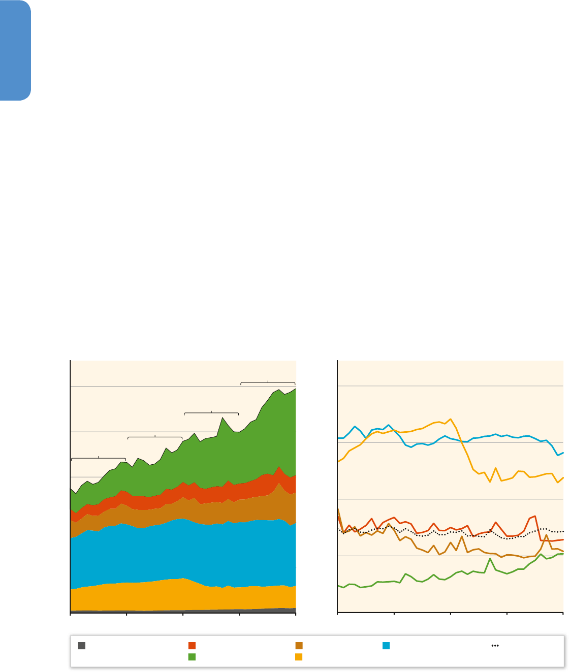
Global per capita GHG emissions (Figure 5.2, right panel) have shown
little trend over the last 40 years. The most noticeable regional trend
over the last two decades in terms of per capita GHG emissions is the
increase in Asia. Per capita emissions in regions other than EIT were
fairly flat until the last several years when per capita emissions have
decreased slightly in Latin America (LAM) and the group of member
countries of the Organisation for Economic Co-operation and Develop-
ment in 1990 (OECD-1990).
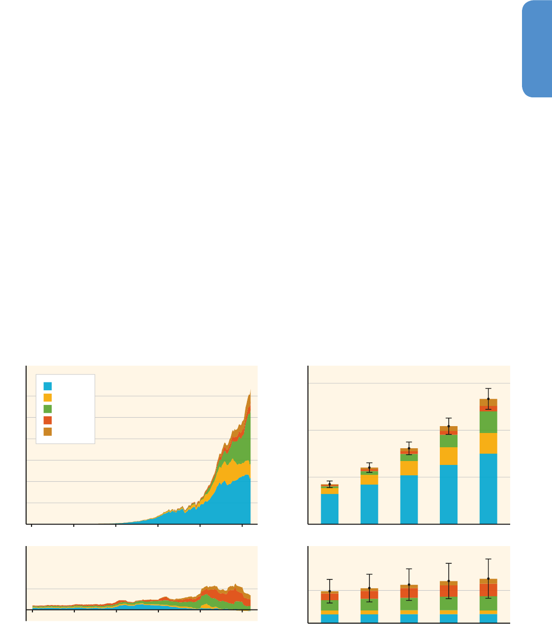
Fossil CO
2
emissions have grown substantially over the past two cen-
turies (Figure 5.3, left panels). Fossil CO
2
emissions over 2002 – 2011
were estimated at 30 ± 8 % GtCO
2
/ yr (Andres etal., 2012), (90 % confi-
dence interval). Emissions in the 2000s as compared to the 1990s were
higher in all regions, except for EIT, and the rate of increase was largest
in ASIA. The increase in developing countries is due to an industrial-
ization process that historically has been energy-intensive; a pattern
similar to what the current OECD countries experienced before 1970.
The figure also shows a shift in relative contribution. The OECD-1990
countries contributed most to the pre-1970 emissions, but in 2010 the
developing countries and ASIA in particular, make up the major share
of emissions.
Figure 5�2 | Left panel: GHG emissions per region over 1970 – 2010. Emissions include all sectors, sources and gases, are territorial (see Box 5.2), and aggregated using 100-year
GWP values. Right panel: The same data presented as per capita GHG emissions. Data from JRC / PBL (2013) and IEA (2012). Regions are defined in Annex II.2.
ASIA
LAM
MAF
OECD-1990
EIT
World
OECD-1990 Countries
Economies in Transition
Latin America and Caribbean
Asia
International Transport Middle East and Africa World Average
0
10
20
30
40
50
Aggregate GHG Emissions [GtCO
2
eq/yr]
1970 1980 1990 2000 2010
0
5
10
15
20
Per Capita GHG Emissions [(tCO
2
eq/cap)/yr]
1970 1980 1990 2000 2010
+2.8%/yr
+1.4%/yr
-3.7%/yr
+0.1%/yr
+2.3%/yr
+0.9%/yr
+0.6%/yr
+0.8%/yr
+0.5%/yr
+1.3%/yr
+0.5%/yr
+3.1%/yr
+1.2%/yr
+0.2%/yr +0.9%/yr
-0.3%/yr
World +2.2%/yr
2000-10
World +0.6%/yr
1990-00
World +1.4%/yr
1980-90
World +2.0%/yr
1970-80
+3.7%/yr
+3.4%/yr
+2.3%/yr
+5.4%/yr
starting in the 1990s and the rapid increase in GHG emissions in Asia
in the 2000s. Emissions values in Section 5.2 are from the Emissions
Database for Global Atmospheric Research (EDGAR) (JRC / PBL, 2013)
unless otherwise noted. As in previous assessments, the EDGAR inven-
tory is used because it provides the only consistent and comprehensive
estimate of global emissions over the last 40 years. The EDGAR emis-
sions estimates for specific compounds are compared to other results
in the literature below.
Similar trends were seen for fossil CO
2
emissions, where a longer
record exists. The absolute growth rate over the last decade was
8 GtCO
2
/ decade, which was higher than at any point in history (Boden
et al., 2012). The relative growth rate for per capita CO
2
emissions
over the last decade is still smaller than the per capita growth rates
at previous points in history, such as during the post-World War II eco-
nomic expansion. Absolute rates of CO
2
emissions growth, however,
are higher than in the past due to an overall expansion of the global
economy due to population growth.
Carbon dioxide (CO
2
) is the largest component of anthropogenic GHG
emissions (Figure 1.3 in Chapter 1). CO
2
is released during the combus-
tion of fossil fuels such as coal, oil, and gas as well as the production of
cement (Houghton, 2007). In 2010, CO
2
, including net land-use-change
emissions, comprised over 75 % (38± 3.8 GtCO
2
eq / yr) of 100-year
GWP-weighted anthropogenic GHG emissions (Figure 1.3). Between
1970 – 2010, global anthropogenic fossil CO
2
emissions more than
doubled, while methane (CH
4
) and nitrous oxide (N
2
O) each increased
by about 45 %, although there is evidence that CH
4
emissions may
not have increased over recent decades (see Section 5.2.3). In 2010,
their shares in total GHG emissions were 16 % (7.8± 1.6 GtCO
2
eq / yr)
and 6.2 % (3.1± 1.9 GtCO
2
eq / yr) respectively. Fluorinated gases,
which represented about 0.4 % in 1970, increased to comprise 2 %
(1.0± 0.2 GtCO
2
eq / yr) of GHG emissions in 2010. Some anthropogenic
influences on climate, such as chlorofluorocarbons and aviation con-
trails, are not discussed in this section, but are assessed in the Inter-
governmental Panel on Climate Change (IPCC) Working Group I (WGI)
contribution to the Fifth Assessment Report (AR5) (Boucher and Ran-
dall, 2013; Hartmann et al., 2013). Forcing from aerosols and ozone
precursor compounds are considered in the next section.
Following general scientific practice, 100-year GWPs from the IPCC
Second Assessment Report (SAR) (Schimel etal., 1996) are used as the
index for converting GHG emission estimates to common units of CO
2
-
equivalent emissions in this section (please refer to Annex II.9.1 for the
exact values). There is no unique method of comparing trends for dif-
ferent climate-forcing agents (see Sections 1.2.5 and 3.9.6). A change
to 20- or 500-year GWP values would change the trends by ± 6 %.
Similarly, use of updated GWPs from the IPCC Fourth Assessment
Report (AR4) or AR5, which change values by a smaller amount, would
not change the overall conclusions in this section. The largest absolute
359359
Drivers, Trends and Mitigation
5
Chapter 5
impact of a change in index values is on the weight given to methane,
whose emission trends are particularly uncertain (Section 5.2.3;
Kirschke etal., 2013).
Global per capita GHG emissions (Figure 5.2, right panel) have shown
little trend over the last 40 years. The most noticeable regional trend
over the last two decades in terms of per capita GHG emissions is the
increase in Asia. Per capita emissions in regions other than EIT were
fairly flat until the last several years when per capita emissions have
decreased slightly in Latin America (LAM) and the group of member
countries of the Organisation for Economic Co-operation and Develop-
ment in 1990 (OECD-1990).
Fossil CO
2
emissions have grown substantially over the past two cen-
turies (Figure 5.3, left panels). Fossil CO
2
emissions over 2002 – 2011
were estimated at 30 ± 8 % GtCO
2
/ yr (Andres etal., 2012), (90 % confi-
dence interval). Emissions in the 2000s as compared to the 1990s were
higher in all regions, except for EIT, and the rate of increase was largest
in ASIA. The increase in developing countries is due to an industrial-
ization process that historically has been energy-intensive; a pattern
similar to what the current OECD countries experienced before 1970.
The figure also shows a shift in relative contribution. The OECD-1990
countries contributed most to the pre-1970 emissions, but in 2010 the
developing countries and ASIA in particular, make up the major share
of emissions.
CO
2
emissions from fossil fuel combustion and industrial processes
made up the largest share (78 %) of the total emission increase
from 1970 to 2010, with a similar percentage contribution between
2000 and 2010. In 2011, fossil CO
2
emissions were 3 % higher than
in 2010, taking the average of estimates from Joint Research Centre
(JRC) / Netherlands Environmental Assessment Agency (PBL) (Olivier
etal., 2013), U. S. Energy Information Administration (EIA), and Car-
bon Dioxide Information Analysis Center (CDIAC) (Macknick, 2011).
Preliminary estimates for 2012 indicate that emissions growth has
slowed to 1.4 % (Olivier etal., 2013) or 2 % (BP, 2013), as compared
to 2012.
Land-use-change (LUC) emissions are highly uncertain, with emis-
sions over 2002 – 2011 estimated to be 3.3 ± 50 – 75 % GtCO
2
/ yr
(Ciais etal., 2013). One estimate of LUC emissions by region is shown
in Figure 5.3, left panel (Houghton etal., 2012), disaggregated into
sub-regions using Houghton (2008), and extended to 1750 using
regional trends from Pongratz etal. (2009). LUC emissions were com-
parable to or greater than fossil emissions for much of the last two
centuries, but are of the order of 10 % of fossil emissions by 2010.
LUC emissions appear to be declining over the last decade, with
some regions showing net carbon uptake, although estimates do not
agree on the rate or magnitude of these changes (Figure 11.6).
Uncertainty estimates in Figure 5.3 follow Le Quéré etal.(2012) and
WGI (Ciais etal., 2013).
Figure 5�2 | Left panel: GHG emissions per region over 1970 – 2010. Emissions include all sectors, sources and gases, are territorial (see Box 5.2), and aggregated using 100-year
GWP values. Right panel: The same data presented as per capita GHG emissions. Data from JRC / PBL (2013) and IEA (2012). Regions are defined in Annex II.2.
ASIA
LAM
MAF
OECD-1990
EIT
World
OECD-1990 Countries
Economies in Transition
Latin America and Caribbean
Asia
International Transport Middle East and Africa World Average
0
10
20
30
40
50
Aggregate GHG Emissions [GtCO
2
eq/yr]
1970 1980 1990 2000 2010
0
5
10
15
20
Per Capita GHG Emissions [(tCO
2
eq/cap)/yr]
1970 1980 1990 2000 2010
+2.8%/yr
+1.4%/yr
-3.7%/yr
+0.1%/yr
+2.3%/yr
+0.9%/yr
+0.6%/yr
+0.8%/yr
+0.5%/yr
+1.3%/yr
+0.5%/yr
+3.1%/yr
+1.2%/yr
+0.2%/yr +0.9%/yr
-0.3%/yr
World +2.2%/yr
2000-10
World +0.6%/yr
1990-00
World +1.4%/yr
1980-90
World +2.0%/yr
1970-80
+3.7%/yr
+3.4%/yr
+2.3%/yr
+5.4%/yr
0
5
0
500
0
500
1000
1500
0
5
10
15
20
25
30
CO
2
FOLU [Gt] CO
2
Fossil, Cement, Flaring [Gt]
CO
2
FOLU [Gt/yr] CO
2
Fossil, Cement, Flaring [Gt/yr]
20001950190018501800 1750-20101750-20001750-19901750-19801750-1970
1750-20101750-20001750-19901750-19801750-1970
1750
200019501900185018001750
OECD-1990
MAF
LAM
ASIA
EIT
Figure 5�3 | Upper-left panel: CO
2
emissions per region over 1750 – 2010, including emissions from fossil fuel combustion, cement production, and gas flaring (territorial, Boden
etal., 2012). Lower-left panel: an illustrative estimate of CO
2
emissions from AFOLU over 1750 – 2010 (Houghton eal., 2012). Right panels show cumulative CO
2
emissions over
selected time periods by region. Whisker lines give an indication of the range of emission results. Regions are defined in Annex II.2.

360360
Drivers, Trends and Mitigation
5
Chapter 5
Cumulative CO
2
emissions, which are a rough measure of the
impact of past emissions on atmospheric concentrations, are also
shown in Figure 5.3 (right panels). About half of cumulative fossil
CO
2
emissions to 2010 were from the OECD-1990 region, 20 % from
the EIT region, 15 % from the ASIA region, and the remainder from
LAM, MAF, and international shipping (not shown). The cumulative
contribution of LUC emissions was similar to that of fossil fuels until
the late 20th century. By 2010, however, cumulative fossil emis-
sions are nearly twice that of cumulative LUC emissions. Note that
the figures for LUC are illustrative, and are much more uncertain
than the estimates of fossil CO
2
emissions. Cumulative fossil CO
2
emissions to 2011 are estimated to be 1340 ± 110 GtCO
2
, while
cumulative LUC emissions are 680 ± 300 GtCO
2
(WGI Table 6.1).
Cumulative uncertainties are, conservatively, estimated across time
periods with 100 % correlation across years. Cumulative per capita
emissions are another method of presenting emissions in the con-
text of examining historical responsibility (see Chapters 3 and 13;
Teng etal., 2011).
Methane is the second most important greenhouse gas, although its
apparent impact in these figures is sensitive to the index used to convert
to CO
2
equivalents (see Section 3.9.6). Methane emissions are due to
a wide range of anthropogenic activities including the production and
transport of fossil fuels, livestock, and rice cultivation, and the decay of
organic waste in solid waste landfills. The 2005 estimate of CH
4
emissions
from JRC / PBL (2013) of 7.3 GtCO
2
eq is 7 % higher than the 6.8GtCO
2
eq
estimates of US EPA (2012) and Höglund-Isaksson etal. (2012), which is
well within an estimated 20 % uncertainty (Section 5.2.3).
The third most important anthropogenic greenhouse gas is N
2
O, which
is emitted during agricultural and industrial activities as well as dur-
ing combustion and human waste disposal. Current estimates are that
about 40 % of total N
2
0 emissions are anthropogenic. The 2005 esti-
mate of N
2
O emissions from JRC / PBL (2013) of 3.0 GtCO
2
eq is 12 %
lower than the 3.4 GtCO
2
estimate of US EPA (2012), which is well
within an estimated 30 to 90 % uncertainty (Section 5.2.3).
In addition to CO
2
, CH
4
, and N
2
O, the F-gases are also greenhouse
gases, and include hydrofluorocarbons, perfluorocarbons, and sulphur
hexafluoride. These gases, sometimes referred to as High Global Warm-
ing Potential gases (‘High GWP gases’), are typically emitted in smaller
quantities from a variety of industrial processes. Hydrofluorocarbons are
mostly used as substitutes for ozone-depleting substances (i. e., chloro-
fluorocarbons (CFCs), hydrochlorofluorocarbons (HCFCs), and halons).
Emissions uncertainty for these gases varies, although for those gases
with known atmospheric lifetimes, atmospheric measurements can be
inverted to obtain an estimate of total global emissions. Overall, the
uncertainty in global F-gas emissions have been estimated to be 20 %
(UNEP, 2012, appendix), although atmospheric inversions constrain
emissions to lower uncertainty levels in some cases (Section 5.2.3).
Greenhouse gases are emitted from many societal activities, with
global emissions from the energy sector consistently increasing the
most each decade over the last 40 years (see also Figure 5.18). A nota-
ble change over the last decade is high growth in emissions from the
industrial sector, the second highest growth by sector over this period.
Subsequent sections of this chapter describe the main trends and driv-
ers associated with these activities and prospects for future mitigation
options.
5�2�2 Trends in aerosols and aerosol / tropos-
pheric ozone precursors
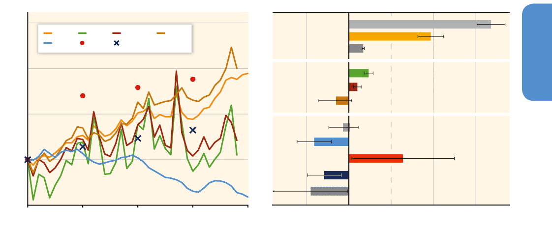
In addition to GHGs, aerosols and tropospheric ozone also contribute
to trends in climate forcing. Because these forcing agents are shorter
lived and heterogeneous, their impact on climate is not discussed in
terms of concentrations, but instead in terms of radiative forcing,
which is the change in the radiative energy budget of the Earth
(Myhre etal., 2014). A positive forcing, such as that due to increases
in GHGs, tends to warm the system while a negative forcing repre-
sents a cooling effect. Trends for the relevant emissions are shown in
the Figure 5.4.
Aerosols contribute a net negative, but uncertain, radiative forc-
ing (IPCC, 2007a; Myhre etal., 2014) estimated to total – 0.90 W / m
2
(5 – 95 % range: – 1.9 to – 0.1 W / m
2
). Trends in atmospheric aerosol
loading, and the associated radiative forcing, are influenced primar-
ily by trends in primary aerosol, black carbon (BC) and organic car-
bon (OC), and precursor emissions (primarily sulphur dioxide (SO
2
)),
although trends in climate and land-use also impact these forcing
agents.
Sulphur dioxide is the largest anthropogenic source of aerosols, and is
emitted by fossil fuel combustion, metal smelting, and other industrial
processes. Global sulphur emissions peaked in the 1970s, and have
generally decreased since then. Uncertainty in global SO
2
emissions
over this period is estimated to be relatively low (± 10 %), although
regional uncertainty can be higher (Smith etal., 2011).
A recent update of carbonaceous aerosol emissions trends (BC and
OC) found an increase from 1970 through 2000, with a particularly
notable increase in BC emissions from 1970 to 1980 (Lamarque etal.,
2010). A recent assessment indicates that BC and OC emissions may
be underestimated (Bond etal., 2013). These emissions are highly sen-
sitive to combustion conditions, which results in a large uncertainty
(+100 % / – 50 %; Bond etal., 2007). Global emissions from 2000 to
2010 have not yet been estimated, but will depend on the trends in
driving forces such as residential coal and biofuel use, which are poorly
quantified, and petroleum consumption for transport, but also changes
in technology characteristics and the implementation of emission
reduction technologies.
Because of the large uncertainty in aerosol forcing effects, the trend in
aerosol forcing over the last two decades is not clear (Shindell etal.,
2013).
Radiative Forcing Components
Radiative Forcing [W m
-2
]
-0.5 0.0 0.5 1.0 1.5
Well Mixed GHGShort Lived GasesAerosols and Precursors
0.75
1.00
1.25
1.75
1.50
1970 1980 1990 2000 2010
Emissions Relative to 1970
Organic Carbon
Black Carbon
NMVOC
CO
N
2
O
CH
4
NH
3
NO
x
SO
2
- 1.2
Aerosol Indirect
CO
2
CH
4
CO NMVOC NO
x
SO
2
BC OC
Figure 5�4 | Left panel: Global trends for air pollutant and methane emissions from anthropogenic and open burning, normalized to 1970 values. Short-timescale variability, in
carbon monoxide (CO) and non-methane volatile organic compounds (NMVOC) in particular, is due to grassland and forest burning. Data from JRC / PBL (2013), except for SO
2
(Smith etal., 2011; Klimont etal., 2013), and BC / OC (Lamarque etal., 2010). Right panel: contribution of each emission species in terms of top of the atmosphere radiative forcing
(adapted from Myhre etal., 2014, Figure 8.17). The aerosol indirect effect is shown separately as there is uncertainty as to the contribution of each species. Species not included in
the left panel are shown in grey (included for reference).
361361
Drivers, Trends and Mitigation
5
Chapter 5
Tropospheric ozone contributes a positive forcing and is formed by
chemical reactions in the atmosphere. Ozone concentrations are
impacted by a variety of emissions, including CH
4
, nitrogen oxides
(NO
x
), carbon monoxide (CO), and volatile organic hydrocarbons (VOC)
(Myhre etal., 2014). Global emissions of ozone precursor compounds
are also thought to have increased over the last four decades. Global
uncertainty has not been quantified for these emissions. An uncertainty
of 10 – 20 % for 1990 NO
x
emissions has been estimated in various
European countries (Schöpp etal., 2005).
5�2�3 Emissions uncertainty
5�2�3�1 Methods for emissions uncertainty estimation
There are multiple methods of estimating emissions uncertainty (Mar-
land etal., 2009), although almost all methods include an element
of expert judgement. The traditional uncertainty estimation method,
which compares emissions estimates to independent measurements,
fails because of a mismatch in spatial and temporal scales. The data
required for emission estimates, ranging from emission factors to
fuel consumption data, originate from multiple sources that rarely
have well characterized uncertainties. A potentially useful input to
uncertainty estimates is a comparison of somewhat independent esti-
mates of emissions, ideally over time, although care must be taken to
assure that data cover the same source categories (Macknick, 2011;
Andres etal., 2012). Formal uncertainty propagation can be useful as
well (UNEP, 2012; Elzen etal., 2013) although one poorly constrained
element of such analysis is the methodology for aggregating uncer-
tainty between regions. Uncertainties in this section are presented as
5 – 95 % confidence intervals, with values from the literature converted
to this range where necessary assuming a Gaussian uncertainty dis-
tribution.
Total GHG emissions from EDGAR as presented here are up to 5 – 10 %
lower over 1970 – 2004 than the earlier estimates presented in AR4
(IPCC, 2007a). The lower values here are largely due to lower estimates
of LUC CO
2
emissions (by 0 – 50 %) and N
2
O emissions (by 20 – 40 %)
and fossil CO
2
emissions (by 0 – 5 %). These differences in these emis-
sions are within the uncertainty ranges estimated for these emission
categories.
5�2�3�2 Fossil carbon dioxide emissions uncertainty
Carbon dioxide emissions from fossil fuels and cement production
are considered to have relatively low uncertainty, with global uncer-
tainty recently assessed to be 8 % (Andres etal., 2012). Uncertainties
in fossil-fuel CO
2
emissions arise from uncertainty in fuel combustion
or other activity data and uncertainties in emission factors, as well as
assumptions for combustion completeness and non-combustion uses.
Default uncertainty estimates (two standard deviations) suggested
by the IPCC (2006) for fossil fuel combustion emission factors are
lower for fuels that have relatively uniform properties (– 3 % / +5 %
for motor gasoline, – 2 % / +1 % for gas / diesel oil) and higher for
most each decade over the last 40 years (see also Figure 5.18). A nota-
ble change over the last decade is high growth in emissions from the
industrial sector, the second highest growth by sector over this period.
Subsequent sections of this chapter describe the main trends and driv-
ers associated with these activities and prospects for future mitigation
options.
5�2�2 Trends in aerosols and aerosol / tropos-
pheric ozone precursors
In addition to GHGs, aerosols and tropospheric ozone also contribute
to trends in climate forcing. Because these forcing agents are shorter
lived and heterogeneous, their impact on climate is not discussed in
terms of concentrations, but instead in terms of radiative forcing,
which is the change in the radiative energy budget of the Earth
(Myhre etal., 2014). A positive forcing, such as that due to increases
in GHGs, tends to warm the system while a negative forcing repre-
sents a cooling effect. Trends for the relevant emissions are shown in
the Figure 5.4.
Aerosols contribute a net negative, but uncertain, radiative forc-
ing (IPCC, 2007a; Myhre etal., 2014) estimated to total – 0.90 W / m
2
(5 – 95 % range: – 1.9 to – 0.1 W / m
2
). Trends in atmospheric aerosol
loading, and the associated radiative forcing, are influenced primar-
ily by trends in primary aerosol, black carbon (BC) and organic car-
bon (OC), and precursor emissions (primarily sulphur dioxide (SO
2
)),
although trends in climate and land-use also impact these forcing
agents.
Sulphur dioxide is the largest anthropogenic source of aerosols, and is
emitted by fossil fuel combustion, metal smelting, and other industrial
processes. Global sulphur emissions peaked in the 1970s, and have
generally decreased since then. Uncertainty in global SO
2
emissions
over this period is estimated to be relatively low (± 10 %), although
regional uncertainty can be higher (Smith etal., 2011).
A recent update of carbonaceous aerosol emissions trends (BC and
OC) found an increase from 1970 through 2000, with a particularly
notable increase in BC emissions from 1970 to 1980 (Lamarque etal.,
2010). A recent assessment indicates that BC and OC emissions may
be underestimated (Bond etal., 2013). These emissions are highly sen-
sitive to combustion conditions, which results in a large uncertainty
(+100 % / – 50 %; Bond etal., 2007). Global emissions from 2000 to
2010 have not yet been estimated, but will depend on the trends in
driving forces such as residential coal and biofuel use, which are poorly
quantified, and petroleum consumption for transport, but also changes
in technology characteristics and the implementation of emission
reduction technologies.
Because of the large uncertainty in aerosol forcing effects, the trend in
aerosol forcing over the last two decades is not clear (Shindell etal.,
2013).
Radiative Forcing Components
Radiative Forcing [W m
-2
]
-0.5 0.0 0.5 1.0 1.5
Well Mixed GHGShort Lived GasesAerosols and Precursors
0.75
1.00
1.25
1.75
1.50
1970 1980 1990 2000 2010
Emissions Relative to 1970
Organic Carbon
Black Carbon
NMVOC
CO
N
2
O
CH
4
NH
3
NO
x
SO
2
- 1.2
Aerosol Indirect
CO
2
CH
4
CO NMVOC NO
x
SO
2
BC OC
Figure 5�4 | Left panel: Global trends for air pollutant and methane emissions from anthropogenic and open burning, normalized to 1970 values. Short-timescale variability, in
carbon monoxide (CO) and non-methane volatile organic compounds (NMVOC) in particular, is due to grassland and forest burning. Data from JRC / PBL (2013), except for SO
2
(Smith etal., 2011; Klimont etal., 2013), and BC / OC (Lamarque etal., 2010). Right panel: contribution of each emission species in terms of top of the atmosphere radiative forcing
(adapted from Myhre etal., 2014, Figure 8.17). The aerosol indirect effect is shown separately as there is uncertainty as to the contribution of each species. Species not included in
the left panel are shown in grey (included for reference).
362362
Drivers, Trends and Mitigation
5
Chapter 5
fuels with more diverse properties (– 15 % / +18 % petroleum coke,
– 10 % / +14 % for lignite). Some emissions factors used by country
inventories, however, differ from the suggested defaults by amounts
that are outside the stated uncertainty range because of local fuel
practices (Olivier etal., 2011). In a study examining power plant emis-
sions in the United States, measured CO
2
emissions were an average
of 5 % higher than calculated emissions, with larger deviations for
individual plants (Ackerman and Sundquist, 2008). A comparison of
five different fossil fuel CO
2
emissions datasets, harmonized to cover
most of the same sources (fossil fuel, cement, bunker fuels, gas flar-
ing) shows ± 4 % differences over the last three decades (Macknick,
2011). Uncertainty in underlying energy production and consumption
statistics, which are drawn from similar sources for existing emission
estimates, will contribute further to uncertainty (Gregg etal., 2008;
Guan etal., 2012).
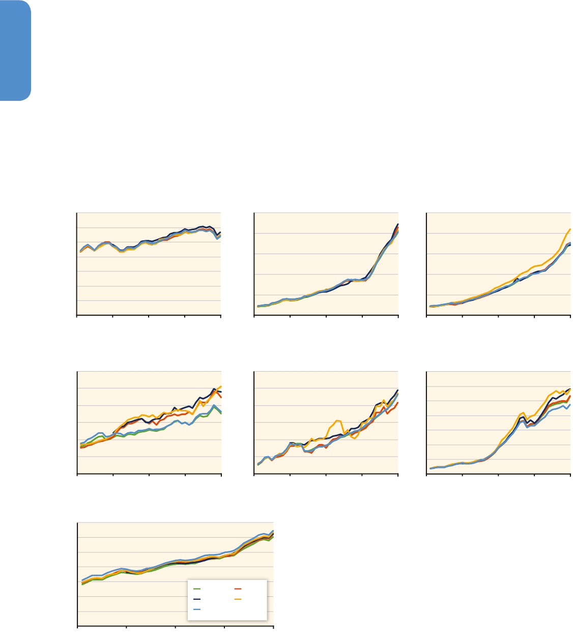
Uncertainty in fossil CO
2
emissions increases at the country level (Mar-
land etal., 1999; Macknick, 2011; Andres etal., 2012), with differences
between estimates of up to 50 %. Figure 5.5 compares five estimates
of fossil CO
2
emissions for several countries. For some countries the
estimates agree well while for others more substantial differences
exist. A high level of agreement between estimates, however, can arise
due to similar assumptions and data sources and does not necessarily
imply an equally low level of uncertainty. Note that differences in
treatment of biofuels and international bunker fuels at the country
level can contribute to differences seen in this comparison.
0
0
2000
4000
6000
8000
10,000
1970 1980 1990 2000 2010
China
0
500
1000
1500
2000
2500
1970 1980 1990 2000 2010
India
100
200
300
400
500
600
1970 1980 1990 2000 2010
Saudi Arabia
0
100
200
300
400
500
600
1970 1980 1990 2000 2010
CO
2
Emissions [MtCO
2
/yr]
South Africa
0
50
100
150
200
250
300
350
1970 1980 1990 2000 2010
Thailand
0
1000
2000
3000
4000
5000
6000
7000
1970 1980 1990 2000 2010
CO
2
Emissions [MtCO
2
/yr]
United States
IEA-S IEA-R
EIA CDIAC
EDGAR
0
5000
10,000
15,000
20,000
25,000
30,000
35,000
1970 1980 1990 2000 2010
CO
2
Emissions [MtCO
2
/yr]
World
Figure 5�5 | Upper panels: five estimates of CO
2
emissions for the three countries with the largest emissions (and complete time series), including fossil fuel combustion, cement
production, and gas flaring. Middle panels: the three countries with the largest percentage variation between estimates. Lower panel: global emissions (MtCO
2
). Emissions data are
harmonized data from Macknick (2011; downloaded Sept 2013), IEA (2012) and JRC / PBL (2013). Note that the vertical scales differ significantly between plots.

363363
Drivers, Trends and Mitigation
5
Chapter 5
5�2�3�3 Other greenhouse gases and non-fossil fuel
carbon dioxide
Uncertainty is particularly large for sources without a simple relation-
ship to activity factors, such as emissions from LUC (Houghton etal.,
2012; see also Chapter 11 for a comprehensive discussion), fugitive
emissions of CH
4
and fluorinated gases (Hayhoe etal., 2002), and bio-
genic emissions of CH
4
and N
2
O, and gas flaring (Macknick, 2011).
Formally estimating uncertainty for LUC emissions is difficult because
a number of relevant processes are not characterized well enough to
be included in estimates (Houghton etal., 2012).
Methane emissions are more uncertain than CO
2
, with fewer global
estimates (US EPA, 2012; Höglund-Isaksson et al., 2012; JRC / PBL,
2013). The relationship between emissions and activity levels for CH
4
are highly variable, leading to greater uncertainty in emission esti-
mates. Leakage rates, for example, depend on equipment design, envi-
ronmental conditions, and maintenance procedures. Emissions from
anaerobic decomposition (ruminants, rice, landfill) also are dependent
on environmental conditions.
Nitrogen oxide emission factors are also heterogeneous, leading to
large uncertainty. Bottom-up (inventory) estimates of uncertainty of
25 % (UNEP, 2012) are smaller than the uncertainty of 60 % estimated
by constraining emissions with atmospheric concentration observation
and estimates of removal rates (Ciais etal., 2013).
Unlike CO
2
, CH
4
, and N
2
O, most fluorinated gases are purely anthropo-
genic in origin, simplifying estimates. Bottom up emissions, however,
depend on assumed rates of leakage, for example, from refrigeration
units. Emissions can be estimated using concentration data together
with inverse modelling techniques, resulting in global uncertainties of
20 – 80 % for various perfluorocarbons (Ivy etal., 2012), 8 – 11 % for
sulphur hexafluoride (SF
6
) (Rigby etal., 2010), and ± 6 – 11 % for HCFC-
22 (Saikawa etal., 2012).
6
5�2�3�4 Total greenhouse gas uncertainty
Estimated uncertainty ranges for GHGs range from relatively low for
fossil fuel CO
2
(± 8 %), to intermediate values for CH
4
and the F-gases
(± 20 %), to higher values for N
2
O (± 60 %) and net LUC CO
2
(50 – 75 %).
Few estimates of total GHG uncertainty exist, and it should be noted
that any such estimates are contingent on the index used to convert
emissions to CO
2
equivalent values. The uncertainty estimates quoted
here are also not time-dependent. In reality, the most recent data is
generally more uncertain due to the preliminary nature of much of the
information used to calculate estimates. Data for historical periods can
also be more uncertain due to less extensive data collection infrastruc-
ture and the lack of emission factor measurements for technologies no
6
HCFC-22 is regulated under the Montreal Protocol but not included in fluorinated
gases totals reported in this chapter as it is not included in the Kyoto Protocol.
longer in use. Uncertainty can also change over time due to changes in
regional and sector contributions.
An illustrative uncertainty estimate of around 10 % for total GHG
emissions can be obtained by combining the uncertainties for each gas
assuming complete independence (which may underestimate actual
uncertainty). An estimate of 7.5 % (90 percentile range) was provided
by the United Nations Environment Programme (UNEP) Gap Report
(UNEP, 2012, appendix), which is lower largely due to a lower uncer-
tainty for fossil CO
2
.
5�2�3�5 Sulphur dioxide and aerosols
Uncertainties in SO
2
and carbonaceous aerosol (BC and OC) emissions
have been estimated by Smith et al. (2011) and Bond et al. (2004,
2007). Sulphur dioxide emissions uncertainty at the global level is rela-
tively low because uncertainties in fuel sulphur content are not well
correlated between regions. Uncertainty at the regional level ranges
up to 35 %. Uncertainties in carbonaceous aerosol emissions, in con-
trast, are high at both regional and global scales due to fundamental
uncertainty in emission factors. Carbonaceous aerosol emissions are
highly state-dependent, with emissions factors that can vary by over
an order of magnitude depending on combustion conditions and emis-
sion controls. A recent assessment indicated that BC emissions may be
substantially underestimated (Bond etal., 2013), supporting the litera-
ture estimates of high uncertainty for these emissions.
5�2�3�6 Uncertainties in emission trends
For global fossil CO
2
, the increase over the last decade as well as previ-
ous decades was larger than estimated uncertainties in annual emis-
sions, meaning that the trend of increasing emissions is robust. Uncer-
tainties can, however, impact the trends of fossil emissions of specific
countries if increases are less rapid and uncertainties are sufficiently
high.
Quantification of uncertainties is complicated by uncertainties not only
in annual uncertainty determinations but also by potential year-to-year
uncertainty correlations (Ballantyne etal., 2010, 2012). For fossil CO
2
,
these correlations are most closely tied to fuel use estimates, an inte-
gral part of the fossil CO
2
emission calculation. For other emissions,
errors in other drivers or emission factors may have their own temporal
trends as well. Without explicit temporal uncertainty considerations,
the true emission trends may deviate slightly from the estimated ones.
In contrast to fossil-fuel emissions, uncertainties in global LUC emis-
sions are sufficiently high to make trends over recent decades uncer-
tain in direction and magnitude (see also Chapter11).
While two global inventories both indicate that anthropogenic meth-
ane emissions have increased over the last three decades, a recent

364364
Drivers, Trends and Mitigation
5
Chapter 5
assessment combining atmospheric measurements, inventories, and
modelling concluded that anthropogenic methane emissions are
likely to have been flat or have declined over this period (Kirschke
etal., 2013). The EDGAR inventory estimates an 86-Mt-CH
4
(or 30 %)
increase over 1980 – 2010 and the EPA (2012) historical estimate has
a 26-Mt-CH
4
increase from 1990 – 2005 (with a further 18-Mt-CH
4
pro-
jected increase to 2010). (Kirschke etal., 2013) derives either a 5-Mt
increase or a net 15-Mt decrease over this period, which indicates
the inventories may be overestimating the increase in anthropogenic
methane emissions. These results suggest that estimates of methane
emission uncertainties of 20 % (UNEP, 2012; Kirschke et al., 2013)
for anthropogenic emissions may be too low, since the differences in
trend between inventories and the inversion synthesis are of this mag-
nitude.
Overall, global SO
2
emissions have decreased over the last two
decades, decreasing again in recent years following an increase from
about 2000 – 2005 (Klimont et al., 2013). Global trends in carbona-
ceous aerosols over the past decade have not been estimated, how-
ever, BC and OC emissions from fuel combustion in China and India
were estimated to have increased over 2000 – 2010 (Lu etal., 2011).
5�2�3�7 Uncertainties in consumption-based carbon
dioxide emission accounts
Consumption-based CO
2
emission accounts reallocate part of the ter-
ritorial CO
2
emissions associated with the production of exports to
the countries where they are eventually consumed (Peters, 2008; Minx
etal., 2009). Different techniques and assumptions have been applied
in modelling consumption-based CO
2
emissions including aggregation
or disaggregation of production sectors (Lenzen, 2011; Lindner etal.,
2012, 2013); consideration of price and deflation effects (Dietzen-
bacher and Hoen, 1998; Dietzenbacher and Wagener, 1999); use of bal-
ancing techniques for data discrepancies (Rey etal., 2004; Lenzen etal.,
2009, 2010); simplifying multi-regional input-output models (Nansai
etal., 2009a); and use of domestic production structure as a proxy for
imports (Suh, 2005). Different models and assumptions result in sub-
stantially different estimates of consumption-based CO
2
emissions, but
a direct comparison between these remains a gap in the literature.
Uncertainties in consumption-based emission accounts arise from
various sources (Lenzen etal., 2010) including (1) uncertainty in the
territory-based emission estimates (see previous sections); (2)uncer-
tainties in input-output and international trade statistics (Lenzen etal.,
2010); and (3)uncertainties in the definitions, level of aggregation, and
assumptions underlying the model (Peters and Solli, 2010; Kanemoto
etal., 2012; Andres etal., 2012).
There has been little quantitative analysis of this at the global level,
with only a few comparisons across different versions of the same
dataset (Andrew and Peters, 2013) and direct comparisons between
studies (Andres etal., 2012). However, there have been detailed stud-
ies at the country level (Lenzen etal., 2010) and many of the mecha-
nisms of uncertainty are understood.
The few quantitative studies on the uncertainty and model spread in
global analyses confirm that the uncertainty in consumption-based
emissions are larger than territorial emissions, though trends over time
are likely to be robust (Andres etal., 2012). The uncertainty in territorial
emission estimates is a key driver for the uncertainty in consumption-
based emissions, and differences in definition and system boundaries
can lead to important differences (Peters and Solli, 2010). A detailed
assessment of the uncertainty due to different supply chain models is
lacking, and this remains a large gap in the literature. Based on model
comparisons, particularly for large countries or regions, the uncertain-
ties may be less important than the uncertainties in territorial emission
estimates used as inputs.
5.3 Key drivers of
global change
5�3�1 Drivers of global emissions
This section analyzes drivers of the global trends in GHG emissions
that were discussed in Section 5.2. In general, drivers are the elements
that directly or indirectly contribute to GHG emissions. While there is
no general consensus in the literature, some researchers distinguish
proximate versus underlying or ultimate drivers (see e. g., Angel etal.,
1998; Geist and Lambin, 2002), where proximate drivers are generally
the activities that are directly or closely related to the generation of
GHGs and underlying or ultimate drivers are the ones that motivate
the proximate drivers.
There is neither a unique method to identify the drivers of climate
change, nor can the drivers always be objectively defined: human
activities manifest themselves through a complex network of inter-
actions, and isolating a clear cause-and-effect for a certain phenom-
enon purely through the lens of scientific observation is often difficult.
Therefore, the term, ‘driver’ may not represent an exact causality but is
used to indicate an association to provide insights on what constitutes
overall changes in global GHG emissions.
In the literature, studies recognize various factors as main drivers to
GHG emissions including consumption (Morioka and Yoshida, 1995;
Munksgaard etal., 2001; Wier etal., 2001; Hertwich and Peters, 2009),
international trade (Weber and Matthews, 2007; Peters and Hertwich,
2008; Li and Hewitt, 2008; Yunfeng and Laike, 2010; Peters etal., 2011;
Jakob and Marschinski, 2013), population growth (Ehrlich and Holdren,
1971; O’Neill etal., 2010), economic growth (Grossman and Krueger,
1994; Arrow et al, 1996; Stern etal., 1996; Lim etal., 2009; Blodgett
and Parker, 2010; Carson, 2010), structural change to a service econ-
0
5
10
15
20
25
30
35
0
2
4
6
8
10
12
1970 1980 1990 2000 2010
0
2
4
6
8
10
12
1970 1980 1990 2000 2010
1970 1980 1990 2000 2010
0
2
4
6
8
10
12
1970 1980 1990 2000 2010
0
2
4
6
8
10
12
1970 1980 1990 2000 2010
0
2
4
6
8
10
12
1970 1980 1990 2000 2010
Fossil Energy CO
2
(Territorial)
Other Industrial Processes
AFOLU
GHG Emissions [GtCO
2
eq/yr] GHG Emissions [GtCO
2
eq/yr]
Asia
World
OECD-1990 Countries Economies in Transition
Latin America and Caribbean Middle East and Africa
Figure 5�6 | Territorial GHG emissions per region over 1970 – 2010. Note that only the bottom-right panel for the World has a different scale for its vertical axis. Fossil energy CO
2
indicates emissions from fossil fuel combustion. Emissions are aggregated using 100-yearGWP values. Data from JRC / PBL (2013) and IEA (2012). Regions are defined in Annex
II.2 | The direct emission data from JRC / PBL (2013) (see Annex II.9) represents land-based CO
2
emissions from forest and peat fires and decay that approximate to CO
2
flux from
anthropogenic emission sources in the FOLU sub-sector. For a more detailed representation of Agriculture and FOLU (AFOLU) GHG flux, see Section 11.2 and Figures 11.2 and 11.6.
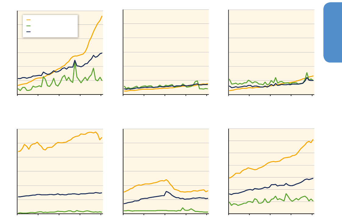
365365
Drivers, Trends and Mitigation
5
Chapter 5
ies at the country level (Lenzen etal., 2010) and many of the mecha-
nisms of uncertainty are understood.
The few quantitative studies on the uncertainty and model spread in
global analyses confirm that the uncertainty in consumption-based
emissions are larger than territorial emissions, though trends over time
are likely to be robust (Andres etal., 2012). The uncertainty in territorial
emission estimates is a key driver for the uncertainty in consumption-
based emissions, and differences in definition and system boundaries
can lead to important differences (Peters and Solli, 2010). A detailed
assessment of the uncertainty due to different supply chain models is
lacking, and this remains a large gap in the literature. Based on model
comparisons, particularly for large countries or regions, the uncertain-
ties may be less important than the uncertainties in territorial emission
estimates used as inputs.
5.3 Key drivers of
global change
5�3�1 Drivers of global emissions
This section analyzes drivers of the global trends in GHG emissions
that were discussed in Section 5.2. In general, drivers are the elements
that directly or indirectly contribute to GHG emissions. While there is
no general consensus in the literature, some researchers distinguish
proximate versus underlying or ultimate drivers (see e. g., Angel etal.,
1998; Geist and Lambin, 2002), where proximate drivers are generally
the activities that are directly or closely related to the generation of
GHGs and underlying or ultimate drivers are the ones that motivate
the proximate drivers.
There is neither a unique method to identify the drivers of climate
change, nor can the drivers always be objectively defined: human
activities manifest themselves through a complex network of inter-
actions, and isolating a clear cause-and-effect for a certain phenom-
enon purely through the lens of scientific observation is often difficult.
Therefore, the term, ‘driver’ may not represent an exact causality but is
used to indicate an association to provide insights on what constitutes
overall changes in global GHG emissions.
In the literature, studies recognize various factors as main drivers to
GHG emissions including consumption (Morioka and Yoshida, 1995;
Munksgaard etal., 2001; Wier etal., 2001; Hertwich and Peters, 2009),
international trade (Weber and Matthews, 2007; Peters and Hertwich,
2008; Li and Hewitt, 2008; Yunfeng and Laike, 2010; Peters etal., 2011;
Jakob and Marschinski, 2013), population growth (Ehrlich and Holdren,
1971; O’Neill etal., 2010), economic growth (Grossman and Krueger,
1994; Arrow et al, 1996; Stern etal., 1996; Lim etal., 2009; Blodgett
and Parker, 2010; Carson, 2010), structural change to a service econ-
0
5
10
15
20
25
30
35
0
2
4
6
8
10
12
1970 1980 1990 2000 2010
0
2
4
6
8
10
12
1970 1980 1990 2000 2010
1970 1980 1990 2000 2010
0
2
4
6
8
10
12
1970 1980 1990 2000 2010
0
2
4
6
8
10
12
1970 1980 1990 2000 2010
0
2
4
6
8
10
12
1970 1980 1990 2000 2010
Fossil Energy CO
2
(Territorial)
Other Industrial Processes
AFOLU
GHG Emissions [GtCO
2
eq/yr] GHG Emissions [GtCO
2
eq/yr]
Asia
World
OECD-1990 Countries Economies in Transition
Latin America and Caribbean Middle East and Africa
Figure 5�6 | Territorial GHG emissions per region over 1970 – 2010. Note that only the bottom-right panel for the World has a different scale for its vertical axis. Fossil energy CO
2
indicates emissions from fossil fuel combustion. Emissions are aggregated using 100-yearGWP values. Data from JRC / PBL (2013) and IEA (2012). Regions are defined in Annex
II.2 | The direct emission data from JRC / PBL (2013) (see Annex II.9) represents land-based CO
2
emissions from forest and peat fires and decay that approximate to CO
2
flux from
anthropogenic emission sources in the FOLU sub-sector. For a more detailed representation of Agriculture and FOLU (AFOLU) GHG flux, see Section 11.2 and Figures 11.2 and 11.6.
omy (Suh, 2006; Nansai etal., 2009b), and energy consumption (Wier,
1998; Malla, 2009; Bolla and Pendolovska, 2011). Each of these topics
will be discussed in more depth, starting in Section 5.3.2.
Obviously many drivers of GHG emissions are interlinked with each
other, and furthermore, many of these drivers can be further decom-
posed into various subcomponents. For example, transportation emis-
sions are an important driver of increasing GHG emissions globally.
But there is a wide regional variation in its significance. Furthermore,
the increase in vehicle miles driven per capita or changes in fuel econ-
omy of average vehicle fleet can also be referred to as a driver, while
these drivers are underlying to the higher-level driver, namely changes
to transportation emissions. Therefore, drivers to GHG emissions can
only be understood in the context of scale, level of detail, and the
framework under which the factors contributing to GHG emissions are
analyzed.
5�3�1�1 Key drivers
Figure 5.6 shows that, globally AFOLU emissions have increased by
12 % between 1970 and 2010. The AFOLU emissions have been more
pronounced in non-OECD-1990 regions and dominate total GHG emis-
sions from MAF and LAM regions. Major increases in global GHG emis-
sion have been, however, associated with CO
2
emissions from fossil
energy (+108 % between 1970 and 2010), which has been growing
more rapidly since AR4 (IPCC, 2007b).
Figure 5.7 shows this increase in fossil energy CO
2
decomposed into
changes in population (+87 %), per capita GDP adjusted with Pur-
chasing Power Parity (PPP) (+103 %), energy intensity in GDP (– 35 %)
and CO
2
intensity of energy (– 15 %) between 1970 and 2010. Over
the last decade, however, the long trend of decreasing carbon inten-
sity in energy has been broken, and it increased by 1.7 %. In short, the
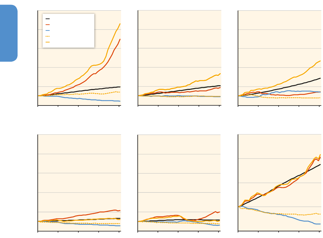
366366
Drivers, Trends and Mitigation
5
Chapter 5
improvements in energy intensity of GDP that the world has achieved
over the last four decades could not keep up with the continuous
growth of global population resulting in a closely synchronous behav-
iour between GDP per capita and CO
2
emission during the period.
At a regional scale, all regions but Asia show 5 % to 25 % reduction in
CO
2
intensity of energy consumption, while Asia increased CO
2
inten-
sity of energy consumption by 44 % between 1970 and 2010. Energy
intensity of GDP declined significantly in the EIT, ASIA, and OECD-1990
(39 % – 55 %) and moderately in LAM (9 %), while in MAF it increased by
41 %. Energy intensity of GDP may increase as an economy enters into
an industrialization process, while it generally decreases as the indus-
trialization process matures and as the share of service sector in the
economy grows (Nansai etal., 2007; Henriques and Kander, 2010). In all
regions, population growth has been a persistent trend. The EIT region
showed the lowest population growth rate over the last four decades
(16 %), whereas MAF marked 188 % increase in population during the
same period. ASIA gained the most to its population from 1.9 billion to
3.7 billion during the period. Purchasing Power Parity (PPP-) adjusted
GDP also grew in all regions ranging from 43 % (MAF), about two-fold
(OECD-1990, EIT, and LAM) to a remarkable six-fold increase (ASIA) over
the last four decades. In general, the use of PPP-adjusted GDP instead of
Market Exchange Rate (MER)-based GDP gives more weight to develop-
ing economies and their GDP growth (Raupach etal., 2007).
In summary, the improvements in energy intensity in GDP over the last
four decades could not keep up with the stable and persistent upward
trends in GDP per capita and population. In particular, a strong growth
in GDP per capita in ASIA combined with its population growth has
been the most significant factors to the increase in GHG emissions dur-
ing the period.
Global CO
2
emissions from fossil energy are decomposed into three
factors using territorial and consumption accounts. Figure 5.8 high-
Figure 5�7 | Four factor decomposition of territorial CO
2
emission from fossil fuel combustion at regional level over 1970 – 2010. Note that only the bottom-right panel for the
World has a different scale for its vertical axis. Data from IEA (2012) and JRC / PBL (2013); based on PPP-adjusted GDP. Regions are defined in Annex II.2.
World
0
2
4
6
8
10
0
2
4
6
8
10
0
2
4
6
8
10
0
2
4
6
8
10
0
2
4
6
8
10
0.5
1.0
1.5
2.0
2.5
1970 1980 1990 2000 2010
1970 1980 1990 2000 2010
1970 1980 1990 2000 2010
1970 1980 1990 2000 2010
1970 1980 1990 2000 2010
1970 1980 1990 2000 2010
OECD-1990 Countries Economies in Transition
Latin America and CaribbeanAsia Middle East and Africa
Population
GDP/cap
Energy/GDP
Fossil Energy CO
2
/Energy
Fossil Energy CO
2
(Territorial)
Index (1=1970)
Index (1=1970)
Index (1=1970)
Index (1=1970)
Index (1=1970)
Index (1=1970)
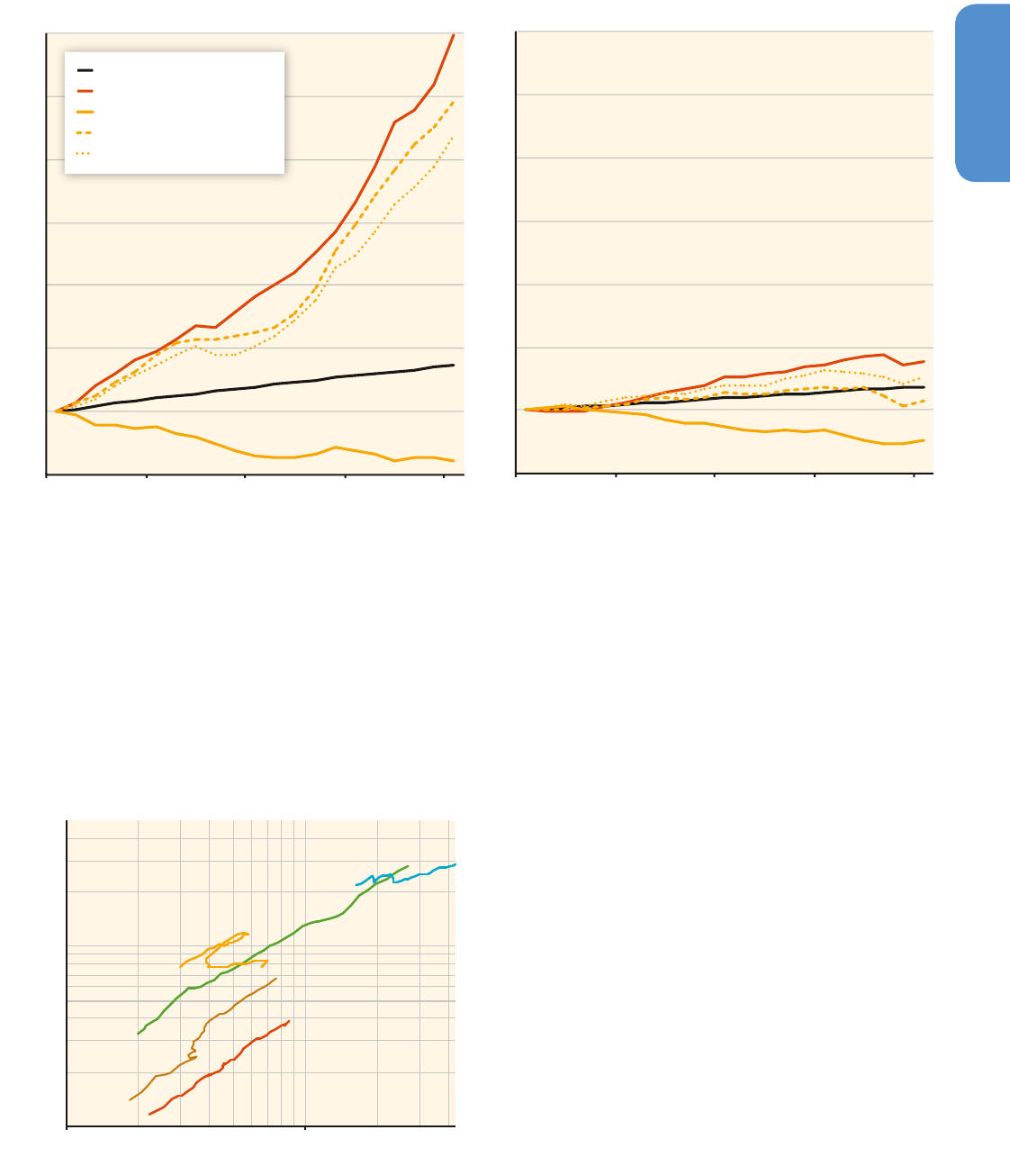
367367
Drivers, Trends and Mitigation
5
Chapter 5
lights the case of ASIA and OECD-1990, where the gap between the
two approaches is largest, over the 1990 – 2010 period. Based on a ter-
ritorial accounting, OECD-1990 increased its CO
2
emissions from fossil
energy only by 6 % from 1990 to 2010. The increase in CO
2
emission
from fossil energy embodied in consumption by OECD-1990, however,
is more significant (22 %) during the period. On the other hand, CO
2
emission embodied in consumption by ASIA increased by 175 % during
the period, while its territorial emissions increased by 197 % during the
period. Increasing international trade played an important role in this
result, which will be elaborated in Section 5.4.
The strong correlation between GDP and CO
2
emissions can be iden-
tified from the historical trajectories of CO
2
emissions and GDP (Fig-
ure 5.9). Although there are notable exceptions (EIT), regional CO
2
emission trajectories are closely aligned with the growth in GDP. On
average, 1 % of world GDP increase has been associated with 0.39 %
increase in fossil energy CO
2
emission during the 1970 – 2010 period.
Over the last two decades, however, 1 % of world GDP increase has
been accompanied with 0.49 % increase in fossil energy CO
2
emission
(1990 – 2010) due largely to the rapid growth of the energy-intensive
non-OECD Asian economy.
Overall, the growth in production and consumption outpaced the
reduction in CO
2
emissions intensity of production and that embodied
in consumption. Together with the growth in population, global CO
2
emissions from fossil energy maintained a stable upward trend, which
characterizes the overall increase in global GHG emissions over the
last two decades.
Figure 5�8 | Three factor decomposition of consumption-based and territorial CO
2
emission from fossil fuel combustion for Asia (left) and OECD (right) over 1990 – 2010. Data from
IEA (2012) and JRC / PBL (2013). Regions are defined in Annex II.2.
0.6
1.0
1.4
1.8
2.2
2.6
3.0
3.4
1990 1995 2000 2005 2010
Population
Gross National Expenditure/cap
Energy CO
2
/Gross National Expenditure
Energy CO
2
(Territory-Based)
Energy CO
2
(Consumption-Based)
0.6
1.0
1.4
1.8
2.2
2.6
3.0
3.4
1990 1995 2000 2005 2010
Asia
OECD-1990 Countries
Index (1=1990)
Index (1=1990)
Figure 5�9 | Regional trajectories of territorial CO
2
emissions from fossil fuel combus-
tion versus GDP over 1970 – 2010. Data from IEA (2012) and JRC / PBL (2013). Regions
are defined in Annex II.2.
ASIA 1970
ASIA 2010
LAM 1970
LAM 2010
MAF 1970
MAF 2010
OECD-1990
1970
OECD-1990
2010
EIT 1970
EIT 2010
400
4000
700 7000
CO
2
Emissions from Fossil Fuel Combustion [Mt/yr]
Gross Domestic Product [Billion Int$
2005
PPP]

368368
Drivers, Trends and Mitigation
5
Chapter 5
5�3�2 Population and demographic structure
5�3�2�1 Population trends
In the second half of the 19th century, global population increased at
an average annual rate of 0.55 %, but it accelerated after 1900. Popu-
lation size and age composition are driven by fertility and mortality
rates, which in turn depend on a range of factors, including income,
education, social norms, and health provisions that keep changing over
time, partly in response to government policies. Section 4.3.1 discusses
these processes in depth. Figure 5.10 presents the main outcomes.
Between 1970 and 2010, global population has increased by 87 %,
from 3.7 billion to 6.9 billion (Wang etal., 2012a). The underlying pro-
cess is the demographic transition in which societies move from a rela-
tively stable population level at high fertility and mortality rates,
through a period of declined mortality rates and fast population
growth, and only at a later stage followed by a decline in fertility rates
with a more stable population size.
Global Population Growth Rate [%/yr]
Population [bn]
0
0.5
1
1.5
2
1850 1875 1900 1925 1950 1975 2000
0
1
2
3
4
5
6
7
Economies in Transition
Middle East and Africa
Asia
OECD-1990 Countries
Latin America
World
Global Growth Rate
Figure 5�10 | Trends in regional and global population growth 1850 – 2010 | Global
data up to 1950 (grey from (UN, 1999). Regional data from 1950 onwards from UN
WPP (2012). Regions are defined in Annex II.2.
Box 5�1 | IPAT and Kaya decomposition methods
The IPAT (Ehrlich and Holdren, 1971) and Kaya (Kaya, 1990) identi-
ties provide two common frameworks in the literature for analyzing
emission drivers by decomposing overall changes in GHG emissions
into underlying factors. The Kaya identity is a special case of the
more general IPAT identity (Ehrlich and Holdren, 1971). The IPAT
identity decomposes an impact (I, e. g., total GHG emissions) into
population (P), affluence (A, e. g., income per capita) and technol-
ogy (T, e. g., GHG emission intensity of production or consumption).
The Kaya identity deals with a subset of GHG emissions, namely
CO
2
emissions from fossil fuel combustion, which is the dominant
part of the anthropogenic GHG emissions and their changes at a
global level (Figure 5.6). While global GHG emissions measured
in GWP100 have increased in all three categories, namely fossil
energy CO
2
, AFOLU, and other over the last four decades, fossil
energy CO
2
dominates the absolute growth of GHG emissions in all
regions and the world during the period. Two approaches to GHG
accounting are distinguished in the literature, namely territorial and
consumption accounts (see Box 5.2 for the definition). The Kaya
identity for territorial CO
2
emissions can be written as:
(1) TerritorialC O
2
emissions =
population ×
GDP
___
population
×
Energy
__
$GDP
×
C O
2
emission
____
Energy
In other words, CO
2
emissions are expressed as a product of
four underlying factors: (1) population, (2)per capita GDP
(GDP / population), (3) energy intensity of GDP (Energy / GDP),
and (4) CO
2
intensity of energy (CO
2
emissions / energy) (Raupach
etal., 2007; Steckel etal., 2011). Also even simpler decomposi-
tion forms can be found in the literature (Raupach etal., 2007).
They are obtained when any two or three adjoining factors in the
four-factor Kaya identity in equation (1) are merged. For example,
merging energy intensity of GDP and CO
2
intensity of energy into
CO
2
intensity of GDP, a three-factor decomposition can be written
as:
(2) TerritorialC O
2
emissions =
population ×
GDP
___
population
×
C O
2
emission
____
GDP
Similarly, consumption-based CO
2
emissions can be decomposed
such that
(3) Consumption − basedC O
2
emissions =
population ×
GNE
___
population
×
consumption − basedC O
2
emission
_________
GNE
In this case, consumption-based CO
2
emissions are decomposed
into (1) population, (2) per capita consumption (GNE / popula-
tion; GNE=Gross National Expenditure), and (3) embodied CO
2
intensity of consumption (consumption-based CO
2
emission / GNE).
The Kaya identity can also be expressed as a ratio between two
time periods to show relative change in CO
2
emissions and its
contributing factors (Raupach etal., 2007).
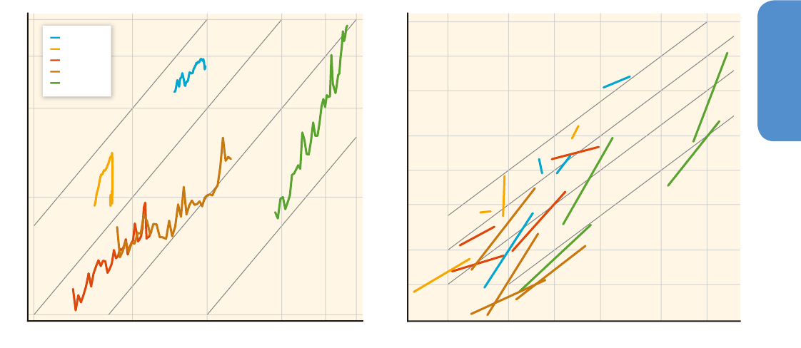
369369
Drivers, Trends and Mitigation
5
Chapter 5
Each person added to the global population increases GHG emis-
sions, but the additional contribution varies widely depending on the
socio-economic and geographic conditions of the additional person.
There is a 91-fold difference in per capita CO
2
emissions from fossil
fuels between the highest and lowest emitters across the nine global
regions analyzed by Raupach etal. (2007). Global CO
2
emissions from
fossil fuel combustion have been growing at about the growth rate
of global population in most of the 1970 – 2010 period, but emissions
growth accelerated toward the end of the period (Figure 5.7).
Aggregating population and GHG emissions data according to the five
IPCC Representative Concentration Pathways (RC) regions (see Annex
II.2), Figure 5.11 shows that between 1971 and 2010 population growth
was fastest in the MAF; GHG emissions have increased most in ASIA
while changes in population and emissions were modest in OECD-1990
and EIT. The evolution of total population and per capita GHG emissions
in the same period is shown in Figure5.11. With some fluctuations, per
capita emissions have declined slightly from rather high levels in the
OECD-1990 countries and the EIT, decreased somewhat from relatively
lower levels in LAM and especially in the MAF, while more than doubled
in ASIA. These trends raise concerns about the future: per capita emis-
sions decline slowly in high-emission regions (OECD-1990 and EIT)
while fast increasing per capita emissions are combined with relatively
fast population and per capita income growth in ASIA (JRC / PBL, 2013).
There is a substantial number of empirical econometric studies that
assess the role of various demographic attributes; an early example is
(Dietz and Rosa, 1997). Those reviewed by O’Neill etal. (2012) confirm
earlier observations that GHG emissions increase with the population
size, although the elasticity values (percent increase in emissions per
1 % increase in population size) vary widely: from 0.32 (Martínez-Zar-
zoso and Maruotti, 2011) to 2.78 (Martínez-Zarzoso etal., 2007) (for
the eight new European Union countries of Central Europe). Differences
in statistical estimation techniques and data sets (countries included,
time horizon covered, the number and kind of variables included in
the regression model and their possible linkages to excluded variables)
explain this wide range. Most recent studies find more than propor-
tional increase of emissions triggered by the increase in population. Yet
the literature presents contradicting results concerning whether popu-
lation growth in rich or poor countries contributes more to increasing
GHG emissions: Poumanyvong and Kaneko (2010) estimate elasticities
ranging from 1.12 (high-income) to 1.23 (middle-income) to 1.75 (low-
income) countries while Jorgenson and Clark (2010) find a value of
1.65 for developed and 1.27 for developing groups of countries.
5�3�2�2 Trends in demographic structure
Urbanization
Income, lifestyles, energy use (amount and mix), and the resulting GHG
emissions differ considerably between rural and urban populations. The
global rate of urbanization has increased from 13 % (1900) to 36 %
(1970) to 52 % (2011), but the linkages between urbanization and
GHG-emissions trends are complex and involve many factors includ-
ing the level of development, rate of economic growth, availability of
energy resources and technologies, and urban form and infrastructure.
1
2
5
20 50 100 200 500 1000
Population [Million]
2
5
10
15
20
GHG Emissions [GtCO
2
eq/yr]
0.2 0.5 1 2 3 4
Population [Billion]
0.1
0.2
0.5
10
20
GHG Emissions [GtCO
2
eq/yr]
1970
2010
1970
2010
1970
2010
1970
2010
1970
2010
CHN
IND
PAK
CHN
IND
IDN
IDN
PAK
BRA
MEX
COL
ARG
BRA
MEX
COL
ARG
NGA
EGY
NGA
ETH
ETH
EGY
IRN
IRN
USA
DEU
TUR
USA
JPN
JPN
DEU
TUR
RUS
UKR
POL
UZB
RUS
UKR
POL
UZB
20 tCO
2
eq/cap/yr
10 tCO
2
eq/cap/yr
5 tCO
2
eq/cap/yr
2 tCO
2
eq/cap/yr
20 tCO
2
eq/cap/yr
10 tCO
2
eq/cap/yr
5 tCO
2
eq/cap/yr
2 tCO
2
eq/cap/yr
OECD-1990
EIT
LAM
MAF
ASIA
Figure 5�11 | Regional trends in population and GHG emissions (left panel) and for each region the four most populous countries in 2010 (right panel). Regions are defined in
Annex II.2 | Grey diagonals connect points with constant emission intensity. Major GHG-emitting regions or countries are in the upper half. A shift to the right presents population
growth. A steep line presents a growth in per capita emissions, while a flat line presents decreasing per capita emissions between 1971 and 2010 | Right panel: The small labels
refer to 1970, the large labels to 2010 | Data from JRC / PBL (2013) and IEA (2012). (Note the log-log plot.)

370370
Drivers, Trends and Mitigation
5
Chapter 5
Comparable direct measures of the effect of urbanization on emissions
remain difficult due to challenges of defining consistent system bound-
aries, including administrative or territorial, functional or economic,
and morphological or land use boundaries. Moreover, because urban
areas are typically much smaller than the infrastructure (e. g., trans-
port, energy) in which they are embedded, strict territorial emissions
accounting such as that used for nations, omits important emissions
sources such as from energy production (Chavez and Ramaswami,
2013). An alternative is to measure the effect of urbanization indirectly,
through statistical analysis of national emission data and its relation
to national urbanization trends. An analysis of the effects of urbaniza-
tion on energy use and CO
2
emissions over the period 1975 – 2005 for
99 countries, divided into three groups based on GDP per capita, and
explicitly considering the shares of industry and services and the energy
intensity in the CO
2
emissions, concludes that the effects depend on
the stage of development. The impact of urbanization on energy use is
negative (elasticity of – 0.132) in the low-income group, while positive
(0.507) in the medium-income group, and strongly positive (0.907) in
the high-income group. Emissions (for given energy use) are positively
affected in all three income groups (between 0.358 and 0.512) (Pou-
manyvong and Kaneko, 2010). Consistent with this conclusion, a set of
multivariate decomposition studies reviewed by O’Neill etal. (2012)
estimate elasticity values between 0.02 and 0.76, indicating almost
negligible to significant but still less than proportional increases in
GHG emissions as a result of urbanization. In China, between 1992
and 2007, urbanization and the related lifestyle changes contributed
to increasing energy-related CO
2
emissions (Minx etal., 2011).
Many studies observe that GHG emissions from urban regions vary
significantly between cities, but that measurements are also widely
dispersed due to differences in accounting methods, the coverage of
GHGs and their sources, and the definition of urban areas (Dhakal,
2009). A comparison of GHG emissions in 10 global cities by consid-
ering geophysical characteristics (climate, resources, gateway status
(port of entry and distribution centre for larger regions due to its geo-
graphic location), and technical features (urban design, electricity gen-
eration, waste processing) finds various outstanding determinants. For
example, the level of household income is important because it affects
the threshold temperature for heating and cooling of the residential
area. The use of high versus low-carbon sources for electricity pro-
duction, such as nuclear power, is an important determinant of urban
GHG emissions in several global cities in the examined sample. Other
determinants include connectivity, accessibility of destination and ori-
gin, and ability to use alternative transportation modes including mass
transit, bicycling, or walking. GHG emissions associated with aviation
and marine fuels reflect the gateway status of cities that, in turn, is
linked to the overall urban economic activity (Kennedy etal., 2009).
An extended analysis of the urbanization-emissions linkage in 88
countries between 1975 and 2003 finds a diverse picture. In 44 coun-
tries, urbanization is found to be not a statistically significant con-
tributor to emissions. In the other 44 countries, all other things equal,
in the early phase of urbanization (at low-urbanization levels) emis-
sions increased, while further urbanization at high-urbanization lev-
els was associated with decreasing emissions (Martínez-Zarzoso and
Maruotti, 2011). This also confirms that in fast-growing and urban-
izing developing countries, urban households tend to be far ahead of
rural households in the use of modern energy forms and use much
larger shares of commercial energy. Urbanization thereby involves
radical increases in household electricity demand and in CO
2
emis-
sions as long as electricity supply comes from fossil fuelled, especially
coal based power plants. Transition from coal to low-carbon electricity
could mitigate the fast increasing CO
2
emissions associated with the
combination of fast urbanization and the related energy transition in
these countries.
The literature is divided about the contribution of urbanization to GHG
emissions. Most top-down studies find increasing emissions as urban-
ization advances, while some studies identify an inverted U-shaped
relationship between the two. Bottom-up studies often identify eco-
nomic structure, trade typology, and urban form as central determi-
nants that are more important than the fraction of people in urban
areas (see Chapter 12). These findings are important to consider when
extrapolating past emission trends, based on past urbanization, to the
future, together with other related aspects.
Age structure and household size
Studies of the effect of age structure (especially ageing) on GHG
emissions fall into two main categories with seemingly contradicting
results: overall macroeconomic studies, and household-level consump-
tion and energy use patterns of different age groups. A national-scale
energy-economic growth model calculates for the United States that
ageing tends to reduce long-term CO
2
emissions significantly relative
to a baseline path with equal population levels (Dalton etal., 2008).
Lower labour force participation and labour productivity would slow
economic growth in an ageing society, leading to lower energy con-
sumption and GHG emissions (O’Neill etal., 2010). In contrast, studies
taking a closer look at the lifestyles and energy consumption of differ-
ent age groups find that older generations tend to use more energy
and emit above average GHGs per person. A study of the impacts of
population, incomes, and technology on CO
2
emissions in the period
1975 – 2000 in over 200 countries and territories finds that the share of
the population in the 15 – 64 age group has a different impact on emis-
sions between different income groups: the impact is negative for high-
income countries and positive for lower-income levels (Fan etal., 2006).
This is consistent with the finding that (in the United States) energy
intensity associated with the lifestyles of the 20 – 34 and the above 65
retirement-age cohorts tends to be higher than that of the 35 – 64 age
group, largely explained by the fact that this middle-age cohort tends
to live in larger households characterized by lower-energy intensity on
a per person basis and that residential energy consumption and elec-
tricity consumption of the 65+ age group tends to be higher (Liddle
and Lung, 2010). Similar results emerge for 14 ‘foundational’ European
Union countries between 1960 and 2000: an increasing share of the
65+ age group in the total population leads to increasing energy con-
sumption although the aggregated data disguise micro-level processes:

371371
Drivers, Trends and Mitigation
5
Chapter 5
ageing may well influence the structure of production, consumption,
transport, social services, and their location (York, 2007). Several stud-
ies assessed above indicate that part of the increasing emissions with
age is due to the differences in household size. A five-country multi-
variate analysis of household energy requirement confirms this (Lenzen
etal., 2006). Immigration is not explicitly considered in these studies,
probably because it does not make much difference.
It remains an open question by how much the household-level effects of
increasing CO
2
emissions as a result of ageing population will counter-
balance the declining emissions as a result of slower economic growth
caused by lower labour force participation and productivity. The balance
is varied and depends on many circumstances. The most important is
changes in labour participation: increasing retirement age in response
to higher life expectancy will keep former retirement-age cohorts (60+)
economically active, which means that the implications of ageing for
incomes, lifestyles, energy use, and emissions are ‘postponed’ and the
ratio of active / retired population changes less. Other important aspects
include the macroeconomic structure, key export and import commodity
groups, the direction and magnitude of financial transfers on the macro
side, and on the health status, financial profile, and lifestyle choices and
possibilities of the elderly at the household level. This makes it difficult
to draw firm conclusions about the ageing-emissions linkages.
Despite the widely varying magnitudes and patterns of household
energy use due to differences in geographical and technological char-
acteristics, lifestyles, and population density, most studies tend to indi-
cate that past trends of increasing age, smaller household size, and
increasing urbanization were positive drivers for increasing energy use,
and associated GHG emissions.
5�3�3 Economic growth and development
5�3�3�1 Production trends
This section reviews the role of income per capita as a driver of emis-
sions while reserving judgement on the appropriateness of GDP per
capita as an indicator of development or welfare (see Kubiszewski
etal., 2013). Global trends in per capita GDP and GHG emissions vary
dramatically by region as shown in Figure 5.12. Economic growth was
strongest in ASIA averaging 5.0 % per annum over the 1970 – 2010
period. Economic growth averaged 1.9 % p. a. in the OECD-1990, but
was below the global average of 1.8 % in the remaining regions. The
MAF and the reforming economies saw setbacks in growth related to
the changing price of oil and the collapse of the centrally planned
economies, respectively. However, all regions showed a decline in
emissions intensity over time. Emissions per capita grew in ASIA and
were fairly constant in LAM, OECD-1990, and EIT, as well as globally,
and declined in MAF. The levels of GDP and emissions per capita also
vary tremendously globally as shown in Figure 5.12.
Per capita emissions are positively correlated with per capita income.
But per capita emissions have declined in all regions but ASIA over
time, so that there has been convergence in the level of per capita
5 kgCO
2
eq/Int$
2005
2 kgCO
2
eq/Int$
2005
1 kgCO
2
eq/Int$
2005
0.5 kgCO
2
eq/Int$
2005
5 kgCO
2
eq/Int$
2005
2 kgCO
2
eq/Int$
2005
1 kgCO
2
eq/Int$
2005
0.5 kgCO
2
eq/Int$
2005
1970
2010
1970
2010
1970
2010
1970
2010
1970
2010
CHN
IDN
IND
PAK
CHN
IDN
IND
PAK
ARG
MEX
BRA
COL
ARG
MEX
BRA
COL
IRN
EGY
NGA
ETH
IRN
EGY
NGA
ETH
USA
DEU
JPN
TUR
USA
DEU
JPN
TUR
POL
RUS
UKR
UZB
POL
RUS
UKR
UZB
OECD-1990
EIT
LAM
MAF
ASIA
2
5
10
20
GHG per Capita [(tCO
2
eq/cap)/yr]
1 2 5 10 20 40
GDP per Capita [(Thousand Int$
2005
/cap)/yr]
1
2
5
10
20
40
GHG per Capita [(tCO
2
eq/cap)/yr]
0.5 1 2 5 10 20 40
GDP per Capita [(Thousand Int$
2005
/cap)/yr]
Figure 5�12 | Regional trends in per capita production and GHG emissions (left panel), and for each region the four most populous countries in 2010 (right panel). Regions
are defined in Annex II.2. Grey diagonals connect points with constant emission intensity (emissions / GDP). A shift to the right presents income growth. A flat or downwards line
presents a decrease in energy intensity, 1971 and 2010. Right panel: The small labels refer to 1970, the large labels to 2010. The figure shows a clear shift to the right for some
countries: increasing income at similar per capita emission levels. The figures also show the high income growth for Asia associated with substantial emissions increase. Data from
JRC / PBL (2013) and IEA (2012).

372372
Drivers, Trends and Mitigation
5
Chapter 5
emissions over time. Despite this convergence, there is still a wide
variation in per capita emissions levels among countries at a common
level of income per capita due to structural and institutional differ-
ences (Pellegrini and Gerlagh, 2006; Matisoff, 2008; Stern, 2012).
The nature of the relationship between growth and the environ-
ment and identification of the causes of economic growth are both
uncertain and controversial (Stern, 2011). The sources of growth are
important because the degree to which economic growth is driven by
technological change versus accumulation of capital and increased
use of resources will strongly affect its impact on emissions. In par-
ticular, growth in developing countries might be expected to be more
emissions-intensive than growth through innovation in technologically
leading developed economies (Jakob et al., 2012). However, despite
this, energy use per capita is strongly linearly correlated with income
per capita across countries (Krausmann etal., 2008; see also Figure
5.15). The short-run effects of growth are slightly different; it seems
that energy intensity rises or declines more slowly in the early stages
of business cycles, such as in the recovery from the global financial
crisis in 2009 – 2010, and then declines more rapidly in the later stages
of business cycles (Jotzo etal., 2012).
Mainstream economic theory (Aghion and Howitt, 2009), and empiri-
cal evidence (e. g., Caselli, 2005) point to technological change and
increases in human capital per worker as the key underlying drivers
of per capita economic output growth in the long run. Technologi-
cal change encompasses both quality improvements in products and
efficiency improvements in production. Human capital is increased
through improving workers’ skills through education and training.
While mainstream growth and development economics does not allo-
cate much role for increasing energy and resource use as drivers of
economic growth (Toman and Jemelkova, 2003), many researchers in
energy and ecological economics do (Stern, 2011).
Productivity is lower in developing countries than developed coun-
tries (Caselli, 2005; Parente and Prescott, 2000). Developing countries
can potentially grow faster than developed countries by adopting
technologies developed elsewhere and ‘catch up’ to the productivity
leaders (Parente and Prescott, 2000). Income per capita has risen in
most countries of the world in the last several decades but there is
much variation over time and regions, especially among low- and
middle-income countries (Durlauf et al., 2005). The highest growth
rates are found for countries that are today at middle-income levels
such as China and India (and before them Singapore, South Korea,
etc.), which are in the process of converging to high-income levels.
But many developing countries have not participated in convergence
to the developed world and some have experienced negative growth
in income per capita. Therefore, there is both convergence among
some countries and divergence among others and a bi-modal distri-
bution of income globally (Durlauf et al., 2005). A large literature
attempts to identify why some countries succeed in achieving eco-
nomic growth and development and others not (Durlauf etal., 2005;
Caselli, 2005; Eberhardt and Teal, 2011). But there seems to be little
consensus as yet (Eberhardt and Teal, 2011). A very large number of
variables could have an effect on growth performance and disentan-
gling their effects is statistically challenging because many of these
variables are at least partially endogenous (Eberhardt and Teal, 2011).
This incomplete understanding of the drivers of economic growth
makes the development of future scenarios on income levels a diffi-
cult task.
Ecological economists such as Ayres and Warr (2009) often ascribe to
energy the central role in economic growth (Stern, 2011). Some eco-
nomic historians, such as Wrigley (2010), Allen (2009), and to some
degree Pomeranz (2000), argue that limited availability of energy
resources can constrain economic growth and that the relaxation of
the constraints imposed by dependence of pre-industrial economies on
biomass energy and muscle power sources alone, with the adoption of
fossil energy was critical for the emergence of the Industrial Revolu-
tion in the 18th and 19th centuries. Stern and Kander (2012) develop
a simple growth model including an energy input and econometri-
cally estimate it using 150 years of Swedish data. They find that since
the beginning of the 19th century constraints imposed on economic
growth by energy availability have declined as energy became more
abundant, technological change improved energy efficiency, and the
quality of fuels improved. A large literature has attempted using time
series analysis to test whether energy use causes economic growth or
vice versa, but results are significantly varied and no firm conclusions
can be drawn yet (Stern, 2011).
Figure 5�13 | Growth rates of per capita income and GHG emissions. The figure shows
the correlation between the average annual growth rate of per capita income and per
capita emissions from 1970 – 2010, for all countries with more than 1 million people by
2010 | Points along the grey lines have either constant emissions intensity or emissions
intensity declining at 2 %, 4 % or 6 % per annum. The size of the circles is proportional
to countries’ emissions. The figure shows that fast growing economies also tend to
have increasing emissions, while slower growing economies tend to have declining per
capita emissions. This is despite quite rapidly declining emissions intensity in some fast
growing economies (upper right corner). Regions are defined in Annex II.2 | Data from
JRC / PBL (2013) and IEA (2012).
Tonnes of CO
2
eq per Year
100 Million
1000 Million
10000 Million
OECD-1990
EIT
LAM
MAF
ASIA
6%/yr Decrease of GHG/GDP
4%/yr Decrease of GHG/GDP
2%/yr Decrease of GHG/GDP
Constant GHG/GDP
-6
-4
-2
0
2
4
Per Capita GHG Annual Growth 1970−2010 [%/yr]
-4 -2 0 2 4 6 8
Per Capita GDP Annual Growth 1970−2010 [%/yr]

373373
Drivers, Trends and Mitigation
5
Chapter 5
The effect of economic growth on emissions is another area of uncer-
tainty and controversy. The environmental Kuznets curve hypothesis pro-
poses that environmental impacts tend to first increase and then even-
tually decrease in the course of economic development (Grossman and
Krueger, 1994). This theory has been very popular among economists but
the econometric evidence has not been found to be very robust (Wag-
ner, 2008; Gallagher, 2009; Vollebergh etal., 2009; Stern, 2010) and in
any case, even early studies found that carbon emissions continue to
rise with increasing income (e. g., Shafik, 1994). More recent research
(Brock and Taylor, 2010) has attempted to disentangle the effects of
economic growth and technological change. Rapid catch-up growth in
middle-income countries tends to overwhelm the effects of emissions-
reducing technological change resulting in strongly rising emissions. But
in developed countries economic growth is slower and hence the effects
of technological change are more apparent and emissions grow slower
or decline. This narrative is illustrated by Figure 5.13. Almost all countries
had declining emissions intensity over time but in more rapidly growing
economies, this was insufficient to overcome the effect of the expansion
of the economy. As a result, though there is much variation in the rate
of decline of emissions intensity across countries, there is, in general,
a strong positive correlation between the rates of growth of emissions
and income per capita. The rapidly growing countries tend to be middle-
and lower-income countries and hence there is a tendency for per capita
emissions to grow in poorer countries and decline in wealthier ones
(Brock and Taylor, 2010).
In conclusion, while economic growth increases the scale of the econ-
omy in the Kaya decomposition and, therefore, should increase emis-
sions, the technological change that is the main underlying driver of
growth tends to reduce emissions. This has resulted in a tendency for
slower growing or declining emissions per capita in wealthier, slower
growing, economies, and global convergence in emissions per capita.
5�3�3�2 Consumption trends
Production and consumption are closely connected, but when we study
their effect on GHG emissions, we find subtle but important differ-
ences. Box 5.2 presents two methods: one for allocating GHG emis-
sions to production (territories), and the other to consumption.
Between 1990 and 2010, emissions from Annex B countries decreased
by 8 % when taking a territorial perspective (production) to carbon
accounting, while over the same period, emissions related to consump-
tion in Annex B increased by 5 % (Wiedmann etal., 2010; Peters etal.,
2011, 2012; Caldeira and Davis, 2011; Andrew et al, 2013). In a similar
vein, as Figure 5.14 shows, while territorial emissions from non-OECD
Asian countries together surpassed those of the OECD-1990 countries
in 2009, for consumption-based emissions, the OECD countries as a
group contributed more than all non-OECD Asian countries together
for every year between 1990 and 2010. The difference between the
two methods also shows up in the trends for the per capita emissions.
The OECD-1990 territorial per capita emissions declined over
1990 – 2010, while consumption-based emissions increased. By 2010,
per capita territorial emissions for OCED countries are three times
those for non-OECD Asian countries, but per capita consumption-
related emissions differ by a factor of five. The overall picture shows a
Box 5�2 | Definitions of territorial and consumption-based emissions
The United Nations Framework Convention on Climate Change
(UNFCCC) requires countries to submit, following the IPCC
guidelines, annual National GHG Emissions Inventories to assess
the progress made by individual countries on GHG emissions and
removals taking place within national (including administered)
territories and offshore areas over which the country has jurisdic-
tion (IPCC, 1997; House of Commons, 2012). These inventories are
called ‘territorial-based emission inventories’.
Consumption-based emissions allocate emissions to the consum-
ers in each country, usually based on final consumption as in the
System of National Accounting but also as trade-adjusted emis-
sions (Peters and Hertwich, 2008; DEFRA, 2012). Conceptually,
consumption-based inventories can be thought of as consumption
equals production minus emissions from the production of exports
(see reviews by (Wiedmann etal., 2007; Wiedmann, 2009; Barrett
etal., 2013). The methodology employed is predominately ‘Multi-
Regional Input-Output Analysis’ (MRIO).
Note on Uncertainty – There is increased uncertainty in consump-
tion-based emission estimates. MRIO datasets combine data from
different data sets, often large and incoherent. As a result, uncer-
tainties arise in relation to calibration, balancing, and harmonisa-
tion; use of different time periods; different currencies; different
country classifications; levels of disaggregation, inflation, and raw
data errors (Lenzen etal., 2004, 2010; Peters, 2007; Weber and
Matthews, 2008; Peters etal., 2012). Production-based emissions
data are a key input to the MRIO models that can vary for some
countries significantly between databases (Peters etal., 2012).
A process of harmonization can greatly reduce the necessary
manipulations, and hence, uncertainties reflected in inconsistent
reporting practices in different countries and regions (Peters and
Solli, 2010; House of Commons, 2012; Barrett etal., 2013). For a
detailed description in the variation of MRIO models, please read
Peters etal.(2012). Peters et al (2012) concludes that estimates
from different studies are robust and that the variation between
estimates relates to different input data and approaches to assign
emissions to trade and not uncertainty.
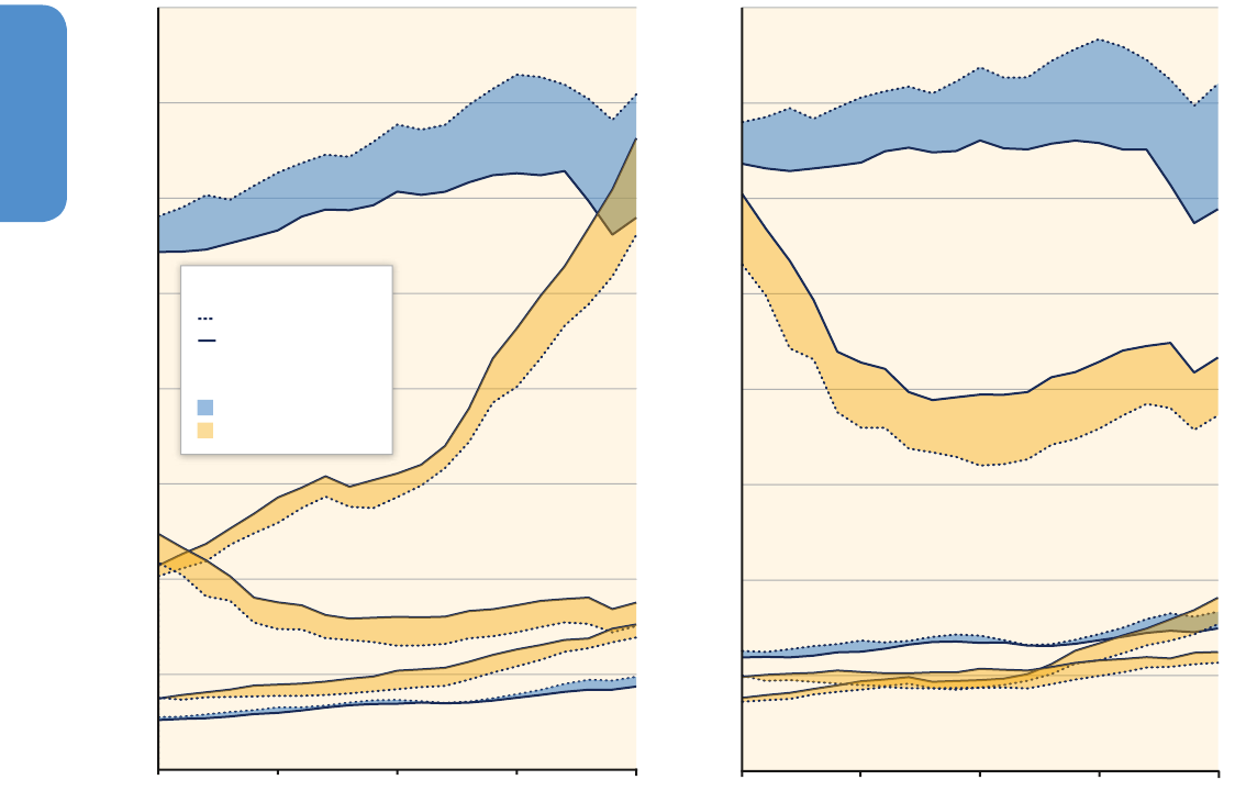
374374
Drivers, Trends and Mitigation
5
Chapter 5
substantial gap between territorial and consumption-based emissions,
due to emissions embedded in trade. For the OECD-1990 countries, the
gap amounts to 2.6 GtCO
2
in 2010. The data shows that the reduction
in territorial emissions that has been achieved in the OECD-1990 coun-
tries has been more than negated by an increase in emissions in other
countries, but related with consumption in OECD-1990 countries. Fur-
thermore, while countries with a Kyoto Protocol commitment did
reduce emissions over the accounting period by 7 %, their share of
imported over domestic emissions increased by 14 % (Peters et al.,
2011; Aichele and Felbermayr, 2012).
Numerous studies have used a structural decomposition analysis to
quantify the factors for changes in GHG emissions over time in both
developed and developing countries (De Haan, 2001; Peters et al.,
2007; Baiocchi and Minx, 2010; Wood, 2009; Weber, 2009). The analy-
sis has been used to separate factors such as the intensity per output,
shifts in production structure, as well as changes in the composition
and the level of consumption. In all of these studies, increasing levels
of consumption is the main contributor to increasing emissions. Specif-
ically, all the studies show that reductions in emissions resulting from
improvements in emissions intensity and changes in the structure of
production and consumption have been offset by significant increases
in emissions, resulting from the volume of consumption, resulting in
an overall increase in emissions (De Haan, 2001; Peters etal., 2007;
Baiocchi and Minx, 2010). For example, De Haan (2001) demonstrates
for the Netherlands that final demand increased by 31 % over 11 years
(1987 – 1998), Peters et al. (2007) demonstrate an increase of con-
sumption by 129 % over 10 years for China, and Baiocchi and Minx
(2010) show for the United Kingdom that final demand increased by
49 % between 1992 and 2004. In all these cases, the increase in final
demand was greater than the emission reduction caused by structural
change and efficiency improvements, leading to an overall increase in
consumption-related emissions.
Calculating emissions based on a consumption-based approach
sketches a more negative view on the decoupling of economic growth
from greenhouse gas emissions. According to York (2007), territorial
emissions showed a relative decoupling; emissions grew by 0.73 % for
every 1 % increase in GDP per capita from 1960 – 2008. However, the
elasticity of consumption-based emissions with respect to economic
Figure 5�14 | Territory-based versus consumption-based CO
2
emissions in five world regions, from 1990 to 2010 | The left panel presents total emissions, while the right panel
presents per capita emissions. The blue areas indicate that a region is a net importer of embodied CO
2
emissions. The yellow area indicates a region is a net exporter of embodied
CO
2
| Data from Lenzen etal. (2010). Regions are defined in Annex II.2.
0
2
4
6
8
10
12
14
16
0
2
4
6
8
10
12
14
16
1990 1995 2000 2005 2010 1990 1995 2000 2005 2010
Annual CO
2
Emissions [GtCO
2
/yr]
Per Capita Annual CO
2
Emissions [(tCO
2
/cap)/yr]
Net Import
Net Export
Territory-Based
Consumption-Based
Attribution Principle
Transfer of Embodied CO
2
OECD-1990
ASIA
EIT
MAF
LAM
EIT
MAF
LAM
OECD-1990
ASIA

375375
Drivers, Trends and Mitigation
5
Chapter 5
growth will have to be revised upwards for OECD-1990 countries,
given that their consumption emissions grew at a faster rate than ter-
ritorial ones (Peters etal., 2011). In this sense, there is less decoupling
in industrialized nations.
5�3�3�3 Structural change
Changes in the structure of the economy — shares of each economic or
industry sector in the output of the economy — might also affect emis-
sions. Over the course of economic development, as income grows,
the share of agriculture in the value of production and employment
tends to decline and the share of services increases (Syrquin and Chen-
ery, 1989). The share of manufacturing tends to follow an inverted
U-shaped path (Hettige etal., 2000). The income levels at which these
transitions occur differ across countries. For example, China’s share
of services in GDP and employment is small and its agriculture share
large, given its income level (World Bank, 2011), while India has a rela-
tively large service sector (Deb Pal etal., 2012). Between 1970 and
2010 the global share of agriculture in GDP has declined from 9 % to
3 % while the share of services increased from 53 % to 71 %. Industry
declined from 38 % to 26 % of GDP (World Bank, 2011). Schäfer (2005)
shows that there are similar changes in the sectoral composition of
energy use. The share of total energy use used in services increases in
the course of economic development while that of industry follows an
inverted U-shaped curve. The share of residential energy use declines
with rising per capita income.
The shift from the industrial sector to services reduces energy use
and emissions less than commonly thought. Partly, this is due to
strong gains in productivity in manufacturing. The productivity gain
can be observed through the price of manufactured goods, which
has historically fallen relative to the price of services. Because of the
price decline, it appears that the share of manufacturing industry
in the economy is falling when, in real output terms, it is constant
or increasing (Kander, 2005). Part of the productivity gain in manu-
facturing is due to improvements in energy efficiency, which reduce
energy intensity in the sector (Kander, 2005). Also, not all service sec-
tors are low in energy intensity. Transport is clearly energy-intensive
and retail and other service sectors depend on energy-intensive infra-
structure.
In Austria and the United Kingdom, the transition of the industrial
society into a service economy or post-industrial society did not lead
to dematerialization (Krausmann et al., 2008), but instead it was
systematically linked to an increase in per capita energy and mate-
rial consumption as all parts of the economy shifted from traditional
to modern methods of production. Further evidence (Henriques and
Kander, 2010) for 10 developed countries (United States, Japan, and
eight European countries), and three emerging economies (India,
Brazil, and Mexico), indicates a minor role for structural change in
reducing energy intensity, while the decline in energy intensity within
industries is found to be the main driver of aggregate energy inten-
sity. Yet the decomposition is sensitive to the level of disaggregation.
A classic result in the growth-accounting literature (Jorgenson and
Griliches, 1967) is that a finer disaggregation of inputs and outputs
leads to lower estimates for technological change and a larger role for
substitution between inputs and structural change. This is confirmed
by Wing (2008), who found that structural change between industries
explained most of the decline in energy intensity in the United States
(1958 – 2000), especially before 1980 (Stern, 2011). An alternative per-
spective is provided by the literature on consumption-based emissions
(see Section5.3.3.2). Baiocchi and Minx (2010) show that the shift
to a service economy in the United Kingdom was partly achieved by
off-shoring emissions-intensive industrial activities and thus reducing
industrial activity, and that the service sector uses imported emissions-
intensive goods. Both of these offset the reduction in emissions from
shifting toward the service sector in the United Kingdom. Likewise, Suh
(2006) and Nansai etal. (2009b) show that if the entire supply chain
is considered, the emissions intensity of services is much higher than if
only the final production of services is considered.
The reform of centrally planned economies has been an important
factor driving changes in GHG emissions. Emissions and energy inten-
sity were high in China, the former Soviet Union, and many Eastern
European countries prior to reform, and declined as their economies
were reformed. China serves as a case in point. Its energy intensity
was very high compared to similar but market-oriented countries
before 1980, but China’s energy intensity decreased sharply between
1980 and 2000, as it opened its economy through market-based
reforms (Ma and Stern, 2008). Energy and emissions intensity rose
and then fell again from 2000 to the present as at first easy options
for energy efficiency improvements were exhausted and later new
policies to improve energy and carbon intensity were put in place.
On the other hand, China’s carbon intensity of energy supply has
increased steadily since at least 1970 (Stern and Jotzo, 2010). Sec-
toral shifts played only a small role in these large movements of the
past three decades (Ma and Stern, 2008; Steckel etal., 2011), though
they were important in the rise in emissions intensity from 2000 to
2005 (Minx etal., 2011).
In conclusion, the role of an increase in share of the service sector in
output in reducing emissions is probably quite small, but finer-grained
structural change could be important and economy-wide reforms con-
tribute much to the adoption of more energy- and emissions-efficient
production processes.
5�3�4 Energy demand and supply
5�3�4�1 Energy demand
Globally, per capita primary energy use, as estimated by the Interna-
tional Energy Agency (IEA) method (see Annex II.9), rose by 31 %
from 1971 – 2010; however the five world regions exhibited two dif-

376376
Drivers, Trends and Mitigation
5
Chapter 5
ferent pathways during this period, as seen in Figure 5.15 (left). In the
OECD-1990 and EIT, energy use per capita rose by 13 – 14 %, while the
other regions increased their per capita energy use at a much higher
rate: LAM by 60 %, MAF by 90 %, and ASIA by 200 %. Nevertheless,
the 2010 per capita energy use in these three regions still remains at
less than half of the OECD-1990 and EIT countries 40 years ago.
The two pathways in per capita energy use are also reflected when
looking at energy intensity over time (Figure 5.15 right). The measure-
ment of energy intensity, i. e., ratio of energy use per unit of GDP and
its limitations, are discussed in the following section. The differences
in pathways between the OECD-1990 and EIT versus ASIA, LAM, and
MAF illustrate the energy intensity gap between the industrialized
and developing countries. In Figure 5.16, we show a similar chart for
individual countries. Combining the left and right panels, we see that
improvements in energy intensity have slowed the growth in energy
use substantially, but have been insufficient to offset the growth in the
scale of the economy (Stern, 2012).
The effects of the oil price shocks in 1973 and 1979 and perhaps 2008
(Hamilton, 2009) are particularly visible as dips in the OECD trend.
These price shocks do not appear, however, to have reversed the
upward trend in per capita primary energy use in the regions. In the
long run, per capita energy consumption has increased with income
and over time since the onset of the Industrial Revolution in Northern
Europe (Gales etal., 2007) and the United States (Grübler, 2008; Tol
etal., 2009) and since the Second World War in southern Europe (Gales
etal., 2007).
Changes in total energy use can be decomposed to reflect the effects
of growth in population and income per capita and changes in energy
intensity, all of which are discussed in detail in other sections of this
chapter as well as in Chapter 7.
The relationship between economic growth and energy use is com-
plicated and variable over time. The provision of energy services is
one of the necessary conditions for economic growth, yet in turn,
economic growth increases the demand for energy services (Grübler
etal., 2012). As income increases, so does energy use. This phenom-
enon, coupled with population growth, has resulted in global total
primary energy use increasing by 130 % between 1971 and 2010,
and almost 50 times since 1800 (Nakicenovic etal., 1998; Grübler,
2008).
5�3�4�2 Energy efficiency and Intensity
Energy efficiency can be defined as the ratio of the desired (usable)
energy output for a specific task or service to the energy input for
the given energy conversion process (Nakicenovic etal., 1996). For
example, for an automobile engine, this is the mechanical energy at
the crankshaft or the wheels divided by the energy input of gasoline.
This definition of energy efficiency is called the first-law efficiency.
Other approaches often define energy efficiency in relative terms, such
as the ratio of minimum energy required by the current best prac-
tice technology to actual energy use, everything else being constant
(Stern, 2012).
Figure 5�15 | Historical trend (1971 – 2010) by region in per capita primary energy (left panel), and primary energy intensity of GDP (right panel), against GDP per capita on the
horizontal axis. Grey diagonals connect points with constant energy intensity (left panel) and constant per capita primary energy use (right panel). Note that both axes are logarith-
mic. Source: IEA (2012); UN WPP (2012); World Bank (2012). Regions are defined in Annex II.2.
OECD-1990
EIT
LAM
MAF
ASIA
20 MJ
/Int$
2005
10 M
J
/Int$
2005
5 MJ /Int$
2005
1971
2010
1971
2010
1971
2010
1971
2010
1971
2010
20
50
100
200
Per Capita Primary Energy [(GJ/cap)/yr]
1 2 5 10 20 40
Per Capita GDP [(Thousand Int$
2005
/cap)/yr]
200 GJ/cap/yr
100 GJ/cap/yr
50 GJ/cap/yr
20 GJ/cap/yr
10 GJ/cap/yr
1971
2010
1971
2010
1971
2010
1971
2010
1971
2010
5
10
20
Primary Energy per GDP [MJ/Int$
2005
]
0.5 1 2 5 10 20 40
Per Capita GDP [(Thousand Int$
2005
/cap)/yr]
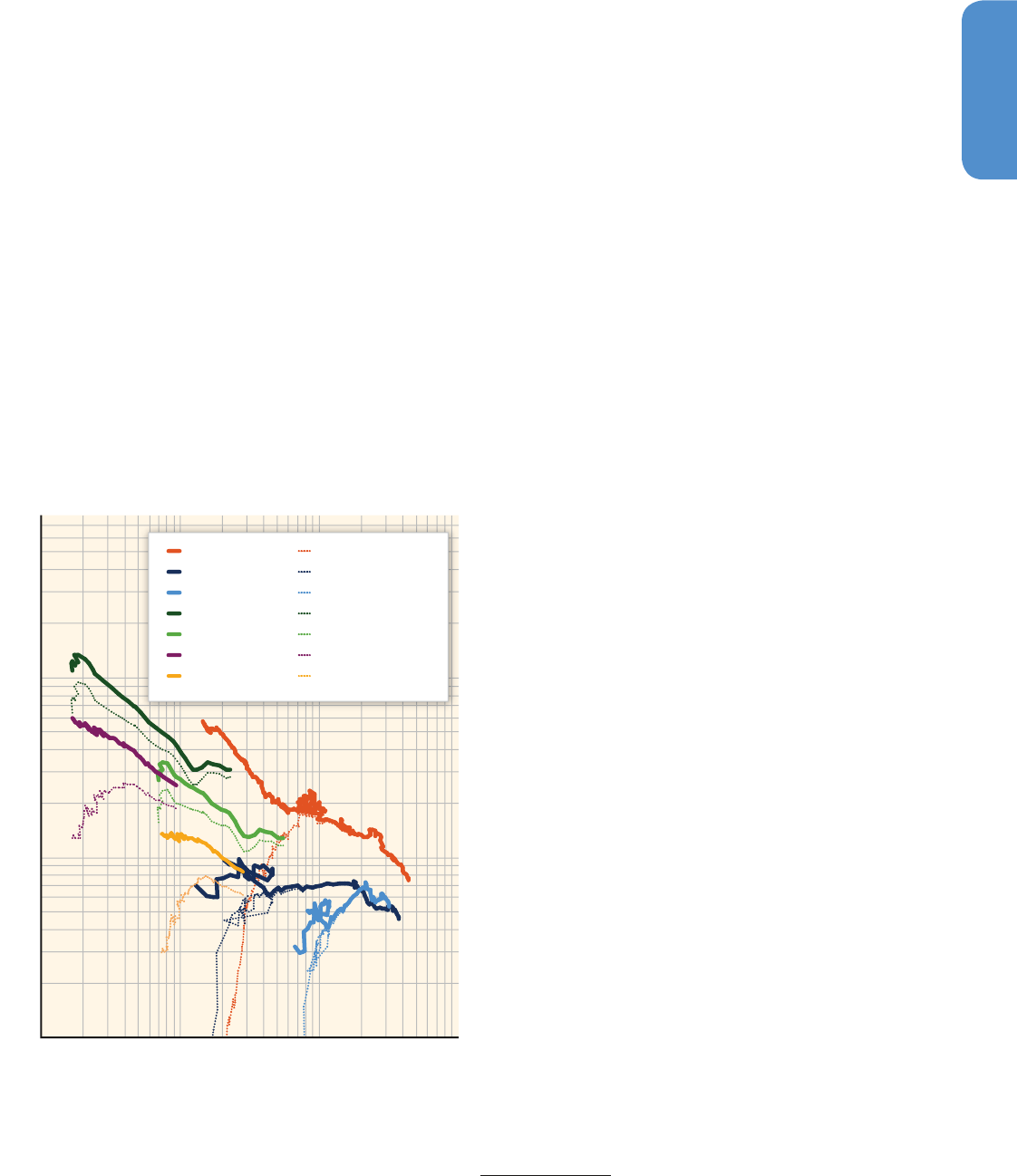
377377
Drivers, Trends and Mitigation
5
Chapter 5
In 2005, the global first-law efficiency of converting primary energy
sources (such as coal or natural gas) to final energy forms (such as
electricity or heat) was about 67 % (i. e., 330 EJ over 496 EJ). The effi-
ciency of further converting final energy forms into useful energy is
lower, with an estimated global average of 51 % (i. e., 169 EJ over 330
EJ). Thus, approximately one-third of global primary energy use is dis-
sipated to the environment in the form of waste heat or what is collo-
quially termed energy ‘losses’ (Grübler etal., 2012).
The theoretical potential for efficiency improvements is thus very large
(Grübler etal., 2012). However, efficiency improvements can lead to
additional demand, a side-effect called the rebound effect, discussed
later in Section 5.6.2, which needs to be taken into account (Pao and
Tsai, 2010).
Economic studies, including those based on the Kaya identity (Naki-
cenovic and Swart, 2000), often use energy intensity — the ratio of
energy use per dollar of GDP — as an indicator of how effectively
energy is used to produce goods and services, also known as its
inverse: the energy productivity. However, energy intensity depends
on many factors other than technical efficiencies, as discussed in the
remainder of this section, and is not an appropriate proxy of actual
energy (conversion) efficiency (Ang, 2006; Filippini and Hunt, 2011;
Stern, 2012; Grübler etal., 2012).
Energy intensity metrics yield valuable insights into potentials for
efficiency improvements related to various activities (Fisher and Naki-
cenovic, 2008; Grübler etal., 2012). Energy intensity measured at the
economy-wide level is an attractive indicator because of its simplic-
ity and ease of comparability across systems and time (e. g., national
economies, regions, cities, etc.). However, the indicator is affected by
a number of issues, including in relation to the way definitions are
made and measurements are performed (Ang, 2006; Filippini and Hunt,
2011). Many factors besides technical efficiency drive energy intensity
differences.
Energy intensities are strongly affected by energy and economic
accounting conventions, which are not always disclosed prominently in
the reporting reference. For energy, the largest influences on the met-
rics are whether primary or final energy are used in the calculations,
and whether or not non-commercial energy
7
is included (Grübler etal.,
2012; see Figure 5.16).
Figure 5.16 illustrates these differences in the evolution of historical
primary energy intensity for four major world economies: China, India,
Japan, and the United States. It shows the different ways energy inten-
sity of GDP can be measured.
To see how the inclusion of non-commercial energy affects energy
intensity, we take the United States as an example, as its PPP and MER
GDP are the same by definition. The thin green curve shows United
States commercial energy intensity. According to Grübler etal. (2012),
commercial energy intensities increase during the early phases of
industrialization, as traditional, less-efficient energy forms are replaced
by commercial energy. Once this substitution is completed, commer-
cial energy intensity peaks and starts to decline. This phenomenon is
sometimes called the ‘hill of energy intensity’ (Grübler etal., 2012).
These peaks are observed to be lower for countries reaching this tran-
sition stage now, promising lower energy intensity in developing coun-
tries that still have to reach the peak (Gales etal., 2007; Lescaroux,
2011; Reddy and Goldemberg, 1990; Nakicenovic etal., 1998). More
important than this ‘hill’ in commercial energy intensities is, however,
a pervasive trend toward overall lower total energy (including also
non-commercial energy) intensities over time and across all countries
(Grübler etal., 2012). It is interesting to note that despite the rela-
tively wide upper and lower bounds of initial energy intensity among
the investigated countries, they all exhibit very similar rates of energy
7
Non-commercial energy is energy that is not commercially traded such as the
traditional biomass or agricultural residues, which are of particular importance in
developing countries.
Figure 5�16 | Energy intensity improvements and per capita GDP — USA (1800 – 2008),
Japan (1885 – 2008), India (1950 – 2008), and China (1970 – 2008). Source: Grübler
etal., 2012. Note: Energy intensities (in MJ per USD) are always shown for total primary
energy (bold lines), and commercial primary energy only (thin lines), and per unit of GDP
expressed at market exchange rates (MER in USD
2005
), and for China, India, and Japan
also at purchasing power parities (PPP in Int$
2005
). For the United States, MER and PPP
are identical.
1
10
100
100 1000 10,000 100,000
Energy Intensity of GDP [MJ/Int$
2005
MER or PPP]
GDP per Capita [Int$
2005
MER or PPP]
USA Total USA Commercial
Japan Total MER Japan Commercial MER
Japan Total PPP Japan Commercial PPP
China Total MER China Commercial MER
China Total PPP China Commercial PPP
India Total MER India Commercial MER
India Total PPP India Commercial PPP

378378
Drivers, Trends and Mitigation
5
Chapter 5
intensity improvements independent of whether they are on a more or
less energy-intensive development trajectory.
The most important accounting factor is the exchange rate used for
converting income measured in local national currencies to inter-
nationally comparable currency units based on either MER or PPP
exchange rates (both illustrated in Figure 5.16) (Grübler etal., 2012).
In the cases of India and China, MER energy intensities are very high,
similar to the energy intensities of the industrialized countries more
than 100 years ago. This gives the appearance of very high energy
intensity of GDP in developing countries. However, China and India’s
PPP-measured GDPs are much higher, meaning that with the same dol-
lar amount, a Chinese or Indian consumer can purchase more goods
and services in developing countries than in industrialized countries.
The PPP-measured energy intensities are thus much lower for devel-
oping countries, indicating substantially higher energy effectiveness in
these countries than would be calculated using MER (Grübler etal.,
2012). A further limitation of GDP accounting, especially for develop-
ing countries, is the exclusion of ‘grey economies’ in official statistics,
which would increase GDP.
Countries with long-term statistical records show improvements in
total energy intensities by a factor of five or more since 1800, corre-
sponding to an global annual average decline of total energy intensi-
ties of about 0.75 – 1 % (Gilli etal., 1990; Fouquet, 2008). Improvement
rates can be much faster over periods of a few decades, as illustrated
in the case of China, which exhibited a steep decline (2 – 3 % / year for
PPP- and MER-based energy intensities, respectively) between 1979
and 2000 before the trend flattened (Stern and Jotzo, 2010). Faster
economic growth leads to a faster turnover of the capital stock of an
economy, thus offering more opportunities to switch to more energy-
efficient technologies. The reverse also applies for the economies in
transition (Eastern Europe and the former Soviet Union in the 1990s)
or recession; that is, with declining GDP, energy intensities increase.
Energy intensity has declined globally in all developed and major
developing countries including India and China (Steckel etal., 2011).
When traditional (non-commercial) biomass fuels are included in the
measure of energy input, energy intensity has declined over time in
most investigated countries (Gales et al., 2007). However, historical
improvements in energy intensities have not been sufficient to fully
offset GDP growth, resulting in increased energy consumption over
time (Bruckner etal., 2010). The literature indicates some albeit incon-
sistent convergence in energy intensities among developed economies,
but not for both developed and developing countries (Le Pen and Sévi,
2010; Mulder and de Groot, 2012).
Changes in energy intensity over time can be decomposed into the
effects of structural change (the shift to more or less energy-inten-
sive industries), changes in the mix of energy sources, technological
change, and the quantities of other inputs such as capital and labour
used (Stern, 2012; Wang, 2011). Globally, structural changes play a
smaller role in determining trends in energy use and CO
2
emissions,
though they can be important in individual countries (Cian et al.,
2013). More generally for countries and regions, energy intensity is
also affected by the substitution of capital and other inputs for energy
(Stern, 2012). The drivers of energy intensity trends are difficult to
isolate. For example, in the United States, most researchers find that
technological change has been the dominant factor in reducing energy
intensity (Metcalf, 2008). Similar results have been found for Sweden
(Kander, 2005) and China (Ma and Stern, 2008; Steckel etal., 2011).
However, Wing (2008) finds that structural change explained most of
the decline in energy intensity in the United States (1958 – 2000), espe-
cially before 1980, and Kaufmann (2004) attributes the greatest part
of the decline to substitution towards higher-quality energy sources,
in particular electricity that produces more output per Joule. Similarly,
Liao etal. (2007) conclude that structural change, instead of techno-
logical change, is the most dominant factor in reducing energy inten-
sity in China.
Some differences in energy intensity among countries are easily
explained. Countries with cold winters and formerly centrally planned
economies tend to be more energy-intensive economies, though the
latter have improved energy intensities significantly in recent decades
through reform of energy markets (Stern, 2012). The role of economic
structure, resource endowments, and policies explain much of the dif-
ferences in energy intensities (Ramachandra et al., 2006; Matisoff,
2008; Wei et al., 2009; Stern, 2012; Davidsdottir and Fisher, 2011).
There is no clear one-to-one link between overall energy intensity and
energy efficiency in production (Filippini and Hunt, 2011), though there
is evidence for the role of energy prices. Higher energy prices are asso-
ciated with lower levels of energy consumption and are significantly
determined by policy. Countries that have high electricity prices tend
to have lower demand for electricity, and vice-versa (Platchkov and
Pollitt, 2011), with a price elasticity of demand for total energy use
between – 0.2 and – 0.45 for the OECD countries between 1978 and
2006 (Filippini and Hunt, 2011).
5�3�4�3 Carbon-intensity, the energy mix, and resource
availability
Carbon intensity is calculated as the ratio of emissions of CO
2
per unit
of primary or final energy, whereas decarbonization refers to the rate
at which the carbon intensity of energy decreases. Throughout the 20th
century, the choice of fossil-fuels for energy has progressed towards
less carbon intensive fuels and to conversion of energy to more usable
forms (e. g., electricity) (Grübler et al., 2012). Hydrogen-rich fuels
release, during combustion, more energy for every carbon atom that is
oxidized to CO
2
(Grübler etal., 1999). The result is a shift from fuels
such as coal with a high-carbon content to energy carriers with a
lower-carbon content such as natural gas
8
, as well as the introduction
of near-zero carbon energy sources, such as renewables, including sus-
8
For further detailed information on carbon emissions for various combustible fuels,
see IPCC (1997) and IPCC (2006).
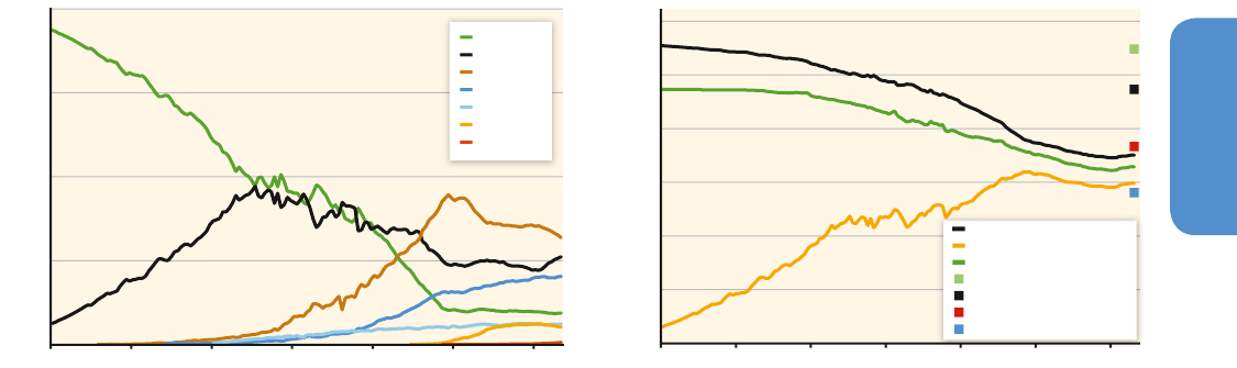
379379
Drivers, Trends and Mitigation
5
Chapter 5
tainably managed biomass (biogenic carbon is reabsorbed through
new growth), and nuclear, and consequently further decarbonization of
energy systems (Grübler and Nakićenović, 1996; Grübler, 2008). Decar-
bonization can also affect the emissions of other GHGs and radiatively
active substances such as aerosols. Figure 5.17 (left panel) shows the
historical dynamics of primary energy. It indicates that the changes in
primary energy are very slow, because it took more than half a century
to replace coal as the dominant source of energy.
Figure 5.17 (right panel) illustrates the historical trend of global
decarbonization of primary energy since 1850 in terms of the aver-
age carbon emissions per unit of primary energy (considering all pri-
mary energy sources, commercial energy sources with and without
biomass). Historically, traditional biomass emissions related to LUCs,
i. e., from deforestation to land for food and energy crops, have far
exceeded carbon releases from energy-related biomass burning, which
indicates that in the past, biomass, like fossil fuels, has also contrib-
uted significantly to increases in atmospheric concentrations of CO
2
(Grübler etal., 2012).
The global rate of decarbonization has been on average about 0.3 %
annually, about six times too low to offset the increase in global
energy use of approximately 2 % annually (Grübler etal., 2012). A sig-
nificant slowing of decarbonization trends since the energy crises of
the 1970s is noteworthy, particularly the rising carbon intensities as a
result of increased use of coal starting in 2000 (IEA, 2009; Stern and
Jotzo, 2010; Steckel etal., 2011). Recent increases in natural gas, in
particular shale gas use, will tend to partially offset the carbonization
trends.
Some future scenarios foresee continuing decarbonization over the
next several decades as natural gas and non-fossil energy sources
increase their share in total primary energy use. Other scenarios antici-
pate a reversal of decarbonization in the long term as more easily
accessible sources of conventional oil and gas are replaced by more
carbon-intensive alternatives such as coal and unconventional oil and
gas (Fisher etal., 2007). Nonetheless, almost all scenarios anticipate an
increase in future demand for energy services. The increase in energy
demand means higher primary energy requirements and, depending on
the rates of future energy-efficiency improvements, higher emissions.
Therefore, energy-efficiency improvements alone will not be sufficient
to significantly reduce GHG emissions, and it is thus essential to accel-
erate the worldwide rate of decarbonization. Current evidence indi-
cates that further decarbonization will not be primarily driven by the
exhaustion of fossil fuels, but rather by economics, technological and
scientific advances, socio-political decisions, and other salient driving
forces. Furthermore, new information and communication technologies
(ICTs) can help reduce the energy needs and associated emissions to
improve the efficiency measures as a result of better management of
energy generation and end-use, e. g., emergence of smart grids and
better control of end-use devices.
Fossil fuel reserves and resources make up the hydrocarbon endow-
ments, which as a whole are not known with a high degree of cer-
tainty. Reserves are the part of global fossil occurrences that are
known with high certainty and can be extracted using current tech-
nologies at prevailing prices. Thus, the quantification and classification
of reserves relies on the dynamic balance between geological assur-
ance, technological possibilities, and economic feasibility. There is little
controversy that oil and gas occurrences are abundant, whereas the
reserves are more limited, with some 50 years of production for oil
and about 70 years for natural gas at the current rates of extraction
(Rogner etal., 2012). Reserve additions have shifted to inherently more
challenging and potentially costlier locations, with technological prog-
ress outbalancing potentially diminishing returns (Nakicenovic etal.,
1998; Rogner etal., 2012).
Figure 5�17 | Left Panel: Structural change in world primary energy (in percent) over 1850 – 2008 illustrating the substitution of traditional biomass (mostly non-commercial) by
coal and later by oil and gas. The emergence of hydro, nuclear and new renewables is also shown. Source: Nakicenovic etal. (1998) and Grübler (2008). Right panel: Decarboniza-
tion of primary energy (PE) use worldwide over 1850 – 2008 (kg of CO
2
emitted per GJ). The black line shows carbon intensities of all primary energy sources, orange line of com-
mercial energy sources without biomass CO
2
emissions, assuming they have all been taken up by the biosphere under a sustainable harvesting regime (biomass re-growth absorbing
the CO
2
released from biomass burning) and the green line shows global decarbonization without biomass and its CO
2
emissions. Note: For comparison, the specific emission
factors (OECD / IPCC default emission factors, lower-heating value (LHV) basis) for biomass (wood fuel), coal, crude oil, and natural gas are also shown (coloured squares). Source:
updated from Grübler etal. (2012).
Biomass
Coal
Oil
Gas
Hydro
Nuclear
Renewables
1850 1875 1900 1925 1950 1975 2000
0
25
50
75
100
1850 1875 1900 1925 1950 1975 2000
Share in World Primary Energy [%]
0
20
40
60
80
100
120
Carbon Intensity [kgCO
2
/GJ]
All PE Carriers and CO
2
Emissions
W/O Biomass CO
2
(but Biomass PE)
W/O Biomass
Biomass 112 kgCO
2
/GJ
Coal 94.6 kgCO
2
/GJ
Oil 73.3 kgCO
2
/GJ
Gas 56.1 kgCO
2
/GJ

380380
Drivers, Trends and Mitigation
5
Chapter 5
In general, estimates of the resources of unconventional gas, oil,
and coal are huge (GEA, 2012; Rogner etal., 2012) ranging for oil
resources to be up to 20,000 EJ or almost 120 times larger than cur-
rent global production; natural gas up to 120,000 EJ or 1300 times
current production, whereas coal resources might be as large as
400,000 EJ or 3500 times larger than current production. However,
global resources are unevenly distributed and are concentrated in
some regions and not others (U. S. Energy Information Administra-
tion, 2010). These upper estimates of global hydrocarbon endow-
ments indicate that their ultimate depletion cannot be the relied
upon to limit global CO
2
emissions. For example, the carbon embed-
ded in oil and gas reserves exceeds the current carbon content of the
atmosphere. The emissions budget for stabilizing climate change at
2 °C above pre-industrial levels is about the same as the current car-
bon content of the atmosphere, meaning that under this constraint
only a small fraction of reserves can be exploited (Meinshausen
etal., 2009). Chapter 7 of this report discusses in detail the current
and future availability of global energy resources (see also Table
7.2).
5�3�5 Other key sectors
This section briefly describes GHG emission trends for the other main
economic sectors (transport, buildings, industry, AFOLU, and waste)
and the correlation between emissions and income, showing marked
differences between sectors and countries. The following sections pro-
vide short discussions of trends and drivers by sector, while the follow-
ing chapters (7 – 11) provide detailed analyses. Note that in Chapter
5, we consider only direct emissions for the buildings sector, whereas
Chapter 9 also includes indirect emissions.
GHG emissions grew in all sectors, except in AFOLU where positive
and negative emission changes are reported across different data-
bases and uncertainties in the data are high (see Section 11.2). As is
clear from Figure 5.18, high-income countries contribute mostly to
emissions associated with transport (Chapter 8) and buildings
(Chapter 9). Low and lower middle-income countries contribute the
largest share of emissions associated with AFOLU (Chapter 11).
Between 2000 and 2010, emissions by upper middle-income coun-
tries from energy (+3.5 GtCO
2
e / yr) and industry (+2.4 GtCO
2
e / yr)
more than doubled, and by 2010, emissions from industry in upper
middle-income countries have passed those from high-income coun-
tries.
The large increase in energy and industry emissions in upper middle-
income countries is consistent with the observed income growth and
the correlation between emissions and income for these sectors (Fig-
ure 5.19). There is a robust positive relation between income and emis-
sions, particularly for annual income levels between 1000 and 10,000
Int$
2005
/ cap, while for transport, the correlation between income and
emissions continues into higher-income levels. We find no positive cor-
relation between income and emissions for AFOLU.
In 2010, the typical high-income country (median of the high-
income group, population-weighted) had per capita emissions of 13
tCO
2
e q/ cap yr, while per capita emissions in the typical low-income
country were only about one-tenth of that value, at 1.4 tCO
2
eq / cap yr.
But, there is a large variation among countries that have similar
income levels. The per capita emissions in high-income countries range
from 8.2 to 21 tCO
2
eq / cap yr, for the (population weighted) 10 and 90
percentile, respectively. Many low-income countries (median income
of 1,200 Int$
2005
/ cap) have low per capita emissions (median of 1.4
tCO
2
eq / yr), but for the low-income country group, average per capita
emissions (4.3 tCO
2
e q/ yr) are pulled up by a few countries with very
high emissions associated with land-use.
5�3�5�1 Transport
Global transport GHG emissions
9
grew from 2.8 GtCO
2
eq in 1970 to
7 GtCO
2
eq in 2010 (JRC / PBL, 2013). The OECD-1990 countries con-
tributed the largest share of the emissions (i. e., 60 % in 1970, 56 %
in 1990, and 46 % in 2010) but the highest growth rates in transport
emissions were in the upper middle-income countries and interna-
tional bunkers. The overall picture shows that transport emissions have
steadily increased but show a marked decrease around 2008 / 2009.
Increasing demand for passenger and freight transport, urban develop-
ment and sprawl, lack of rail and bus transit and cycle infrastructure in
many regions, transport behaviour constrained by lack of modal choice
in some regions, a high fuel-consuming stock of vehicles, relatively low
oil prices, and the limited availability of low-carbon fuels have been the
principal drivers of transport sector CO
2
emission growth over the past
few decades (Jolley, 2004; Davies etal., 2007; IPCC, 2007; Timilsina and
Shrestha, 2009; Ubaidillah, 2011; Wang etal., 2011 Chapter 8).
The marked growth rate of international transport emissions after
2002 coincides with growth in Chinese exporting industries sugges
3ting an influence of trade policies and world trade agreements on
transport emissions (Olivier etal., 2011).
The high oil prices of 2008 and the global recession in 2009 both
resulted in a decrease in fossil fuel consumption for the OECD coun-
tries, with CO
2
emissions declining by 2.0 % in 2008, and an esti-
mated 6.3 % in 2009. GHG emissions in non-OECD countries were not
affected (US EIA, 2011).
There is a strong correlation between per capita transport emissions
and per capita incomes and alignment of the two variables is sharper
in the high-income countries (Figure 5.19) as the demand for personal
transportation increases as standards of living rise and economic activ-
ity increases (US EIA, 2011).
9
Consisting of direct CO
2
, CH
4
, N
2
O, and F-gases (Freight Vision, 2009).
Figure 5�18 | Regional and sector distribution of GHG emission trends. Regions are defined in Annex II.2 | The figure shows annual GHG emissions for the six key sectors discussed
in Sections 5.3.4 and 5.3.5 | The left-lower panel presents global sector emissions to assess the relative contribution. Decadal growth rates are projected on the charts for emissions
exceeding 0.2 GtCO
2
eq / yr. The direct emission data from JRC / PBL (2013) and IEA (2012) (see Annex II.9) represents land-based CO
2
emissions from forest and peat fires and decay
that approximate to CO
2
flux from anthopogenic emission sources in the Forestry and Other Land Use (FOLU) sub-sector. For a more detailed representation of Agriculture and FOLU
(AFOLU) GHG flux see Section 11.2 and Figures 11.2 and 11.6.
AFOLU Industry
Buildings
Transport
Energy Waste
+41%
+27%
+18%
+36%
+35%
+25%
+25%
+18%
+9%
+5%
-1%
+9%
+15%
-4%
+2%
+45%
+27% +26% +9%
+13%
+11%
+11%
-11%
+8%
+67%
0%
+22%
+46%
+61%
+52%
+46%
+95%
+58%
+62%
−8%
+20%
+25%
+11%
+17%
−2%
+13%
+13%
+36%
+31%
+43%
+29%
+48%
+78%
+38%
+50%
+52%
+48%
+57%
−6%
+40%
+30%
+19%
+21%
−3%
+42%
+26%
+4%
+50%
+43%
+38%
−10%
+46%
+63%
−1%
−36%
−4%
−12%
−9%
+10%
−3%
+10%
+43%
−1%
+58%
+66%
+18%
+18%
+100%
+24%
−24%
−2%
+23%
−4%
−17%
−6%
−7%
−4%
+11%
−23%
+22%
+24%
+27%
+4%
+13%
+10%
+8%
−14%
+13%
+14%
+7%
−19%
−41%
+30%
−3%
−2%
−11%
+33%
+25%
+31%
+37%
+35%
+37%
+33%
+22%
+19%
+14%
−20%
−10%
0
5
10
15
20
0
2
4
6
8
0
1
2
3
0
2
4
6
8
0
5
10
15
0
0.5
1
1.5
0
10
20
30
40
50
1970 1980 1990 2000 2010
Annual GHG Emissions [GtCO
2
eq/yr]Annual GHG Emissions [GtCO
2
eq/yr] Annual GHG Emissions [GtCO
2
eq/yr]
1970 1980 1990 2000 2010
Annual GHG Emissions [GtCO
2
eq/yr]
1970 1980 1990 2000 2010
Annual GHG Emissions [GtCO
2
eq/yr]
1970 1980 1990 2000 2010
Annual GHG Emissions [GtCO
2
eq/yr]
1970 1980 1990 2000 2010
1970 1980 1990 2000 2010
Annual GHG Emissions [GtCO
2
eq/yr]
1970 1980 1990 2000 2010
International Transport
Low−Income Countries
Lower−Middle−Income Countries
Upper−Middle−Income Countries
High−Income Countries from Non−OECD-1990
High−Income Countries from OECD-1990
AFOLU
World by Sector
Energy Transport
Buildings Industry
Waste
All +24%
2000-10
All +5%
1990-00
All +14%
1980-90
All +21%
1970-80
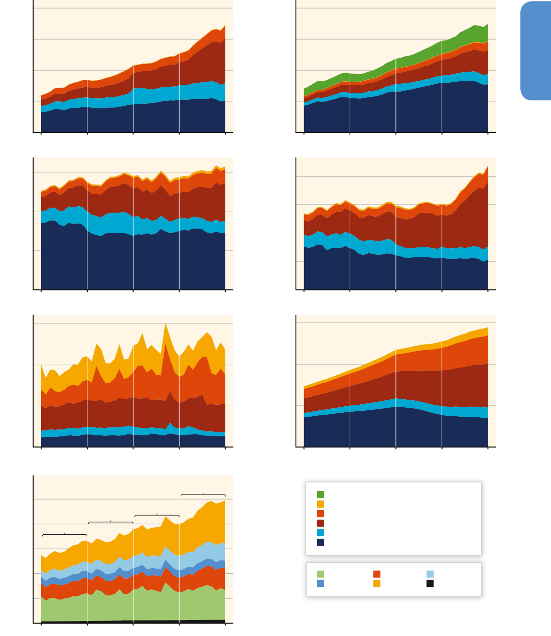
381381
Drivers, Trends and Mitigation
5
Chapter 5
In general, estimates of the resources of unconventional gas, oil,
and coal are huge (GEA, 2012; Rogner etal., 2012) ranging for oil
resources to be up to 20,000 EJ or almost 120 times larger than cur-
rent global production; natural gas up to 120,000 EJ or 1300 times
current production, whereas coal resources might be as large as
400,000 EJ or 3500 times larger than current production. However,
global resources are unevenly distributed and are concentrated in
some regions and not others (U. S. Energy Information Administra-
tion, 2010). These upper estimates of global hydrocarbon endow-
ments indicate that their ultimate depletion cannot be the relied
upon to limit global CO
2
emissions. For example, the carbon embed-
ded in oil and gas reserves exceeds the current carbon content of the
atmosphere. The emissions budget for stabilizing climate change at
2 °C above pre-industrial levels is about the same as the current car-
bon content of the atmosphere, meaning that under this constraint
only a small fraction of reserves can be exploited (Meinshausen
etal., 2009). Chapter 7 of this report discusses in detail the current
and future availability of global energy resources (see also Table
7.2).
5�3�5 Other key sectors
This section briefly describes GHG emission trends for the other main
economic sectors (transport, buildings, industry, AFOLU, and waste)
and the correlation between emissions and income, showing marked
differences between sectors and countries. The following sections pro-
vide short discussions of trends and drivers by sector, while the follow-
ing chapters (7 – 11) provide detailed analyses. Note that in Chapter
5, we consider only direct emissions for the buildings sector, whereas
Chapter 9 also includes indirect emissions.
GHG emissions grew in all sectors, except in AFOLU where positive
and negative emission changes are reported across different data-
bases and uncertainties in the data are high (see Section 11.2). As is
clear from Figure 5.18, high-income countries contribute mostly to
emissions associated with transport (Chapter 8) and buildings
(Chapter 9). Low and lower middle-income countries contribute the
largest share of emissions associated with AFOLU (Chapter 11).
Between 2000 and 2010, emissions by upper middle-income coun-
tries from energy (+3.5 GtCO
2
e / yr) and industry (+2.4 GtCO
2
e / yr)
more than doubled, and by 2010, emissions from industry in upper
middle-income countries have passed those from high-income coun-
tries.
The large increase in energy and industry emissions in upper middle-
income countries is consistent with the observed income growth and
the correlation between emissions and income for these sectors (Fig-
ure 5.19). There is a robust positive relation between income and emis-
sions, particularly for annual income levels between 1000 and 10,000
Int$
2005
/ cap, while for transport, the correlation between income and
emissions continues into higher-income levels. We find no positive cor-
relation between income and emissions for AFOLU.
Figure 5�18 | Regional and sector distribution of GHG emission trends. Regions are defined in Annex II.2 | The figure shows annual GHG emissions for the six key sectors discussed
in Sections 5.3.4 and 5.3.5 | The left-lower panel presents global sector emissions to assess the relative contribution. Decadal growth rates are projected on the charts for emissions
exceeding 0.2 GtCO
2
eq / yr. The direct emission data from JRC / PBL (2013) and IEA (2012) (see Annex II.9) represents land-based CO
2
emissions from forest and peat fires and decay
that approximate to CO
2
flux from anthopogenic emission sources in the Forestry and Other Land Use (FOLU) sub-sector. For a more detailed representation of Agriculture and FOLU
(AFOLU) GHG flux see Section 11.2 and Figures 11.2 and 11.6.
AFOLU Industry
Buildings
Transport
Energy Waste
+41%
+27%
+18%
+36%
+35%
+25%
+25%
+18%
+9%
+5%
-1%
+9%
+15%
-4%
+2%
+45%
+27% +26% +9%
+13%
+11%
+11%
-11%
+8%
+67%
0%
+22%
+46%
+61%
+52%
+46%
+95%
+58%
+62%
−8%
+20%
+25%
+11%
+17%
−2%
+13%
+13%
+36%
+31%
+43%
+29%
+48%
+78%
+38%
+50%
+52%
+48%
+57%
−6%
+40%
+30%
+19%
+21%
−3%
+42%
+26%
+4%
+50%
+43%
+38%
−10%
+46%
+63%
−1%
−36%
−4%
−12%
−9%
+10%
−3%
+10%
+43%
−1%
+58%
+66%
+18%
+18%
+100%
+24%
−24%
−2%
+23%
−4%
−17%
−6%
−7%
−4%
+11%
−23%
+22%
+24%
+27%
+4%
+13%
+10%
+8%
−14%
+13%
+14%
+7%
−19%
−41%
+30%
−3%
−2%
−11%
+33%
+25%
+31%
+37%
+35%
+37%
+33%
+22%
+19%
+14%
−20%
−10%
0
5
10
15
20
0
2
4
6
8
0
1
2
3
0
2
4
6
8
0
5
10
15
0
0.5
1
1.5
0
10
20
30
40
50
1970 1980 1990 2000 2010
Annual GHG Emissions [GtCO
2
eq/yr]Annual GHG Emissions [GtCO
2
eq/yr] Annual GHG Emissions [GtCO
2
eq/yr]
1970 1980 1990 2000 2010
Annual GHG Emissions [GtCO
2
eq/yr]
1970 1980 1990 2000 2010
Annual GHG Emissions [GtCO
2
eq/yr]
1970 1980 1990 2000 2010
Annual GHG Emissions [GtCO
2
eq/yr]
1970 1980 1990 2000 2010
1970 1980 1990 2000 2010
Annual GHG Emissions [GtCO
2
eq/yr]
1970 1980 1990 2000 2010
International Transport
Low−Income Countries
Lower−Middle−Income Countries
Upper−Middle−Income Countries
High−Income Countries from Non−OECD-1990
High−Income Countries from OECD-1990
AFOLU
World by Sector
Energy Transport
Buildings Industry
Waste
All +24%
2000-10
All +5%
1990-00
All +14%
1980-90
All +21%
1970-80
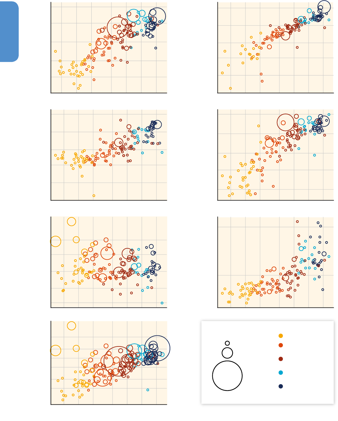
382382
Drivers, Trends and Mitigation
5
Chapter 5
0.05
0.2
1
5
20
Per Capita GHG Emissions [(tCO
2
eq/cap)/yr]
0.5 1 2 5 10 20 40
0.01
0.05
0.2
1
5
Per Capita GHG Emissions [(tCO
2
eq/cap)/yr]
0.5 1 2 5 10 20 40
0.01
0.05
0.2
1
5
Per Capita GHG Emissions [(tCO
2
eq/cap)/yr]
0.5 1 2 5 10 20 40
0.01
0.05
0.2
1
5
Per Capita GHG Emissions [(tCO
2
eq/cap)/yr]
0.5 1 2 5 10 20 40
0.05
0.2
1
5
20
Per Capita GHG Emissions [(tCO
2
eq/cap)/yr]
0.5 1 2 5 10 20 40
0.2
1
Per Capita GHG Emissions [(tCO
2
eq/cap)/yr]
0.5 1 2 5 10 20 40
1
2
5
10
20
50
Per Capita GHG Emissions [(tCO
2
eq/cap)/yr]
0.5 1 2 5 10 20 40
Per Capita Income [Thousand Int$
2005
/yr]
Energy Transport
Buildings
AFOLU Waste
ALL Sectors
Industry
Tonnes of CO
2
eq per Year
100 Million
1000 Million
10000 Million
High-Income Countries
from OECD-1990
High-Income Countries
from Non-OECD-1990
Upper-Middle-Income
Countries
Lower-Middle-Income
Countries
Low-Income Countries
⇒

383383
Drivers, Trends and Mitigation
5
Chapter 5
5�3�5�2 Buildings
Building sector emissions grew from 2.5 GtCO
2
eq in 1970 to
3.2 GtCO
2
eq in 2010 with emissions growth rates in OECD-1990 coun-
tries being largely negative. Positive-emission growth rates were reg-
istered in the upper and lower middle-income countries, although the
largest contribution to buildings emissions still came from OECD-1990
countries (Figure 5.18).
Per capita buildings emissions and per capita income are positively
correlated. Considering a life-cycle assessment starting with manufac-
turing of building materials to demolition, over 80 % of GHG emissions
take place during the building operation phase (UNEP, 2009) largely
from consumption of electricity for heating, ventilation, and air condi-
tioning (HVAC), water heating, lighting, and entertainment (US DOE,
2008). On average, most residential energy in developed countries is
consumed for space heating, particularly in cold climates. 58 % of the
demand for energy in buildings was contributed by space heating in
1990 and 53 % in 2005, while water heating contributed 17 % in 1990
and 16 % in 2005, appliances 16 % and 21 %, respectively, and cook-
ing and lighting about 5 % (IEA, 2008; UNEP, 2009). In low-income
countries, a large proportion of operational energy is derived from pol-
luting fuels, mainly wood and other biomass, such as dung and crop
residues, and a high number of people (2.4 billion) still use biomass for
cooking and heating (International Energy Agency, 2002, 2006).
5�3�5�3 Industry
Direct emissions from industry (excluding waste / waste water
and AFOLU contributions
10
) grew from 5.4 GtCO
2
eq / yr in 1970 to
8.8 GtCO
2
eq / yr in 2010. The contribution of OECD countries dominated
these emissions at the start of the period with over 57 % of the total
but declined to 24 % of the total in 2010. The middle-income coun-
tries have become the major emitters, particularly after 2000 (Figure
5.18) when the annual growth rate in emissions increased very sig-
nificantly in the middle income countries. There is a positive correlation
between per capita emissions from industry and per capita income up
to an income level of 10,000 Int$
2005
/ cap. Beyond that income level, the
correlation decreases due to improvements in energy efficiency in the
industrialized OECD countries (European Environment Agency, 2009).
10
Industry emissions including emissions from waste and waste water are reported
in Section 10.2 in Chapter 10.
Energy use in industry, which is the major source of emissions from
the sector, has grown in both absolute and relative terms in the OECD-
1990 region and in relative terms in EIT countries driven by changes
in income, the level of industrial output, fuel switching, and structural
changes (International Energy Agency, 2003). There has also been a
complex restructuring and relocation of the production and consump-
tion of goods and supply of services that has shaped the location of
industrial emissions, resulting in the shift of emissions to some non-
OECD Asian economies (De Backer and Yamano, 2012; Backer and
Yamano, 2007).
The production of energy-intensive industrial goods including cement,
steel, aluminium has grown dramatically. From 1970 to 2012, global
annual production of cement increased 500 %; aluminium 400 %;
steel 150 %, ammonia 250 %; and paper 200 % (USGS, 2013); with
energy-intensive industries increasingly being located in developing
nations (IPCC, 2007a). Rapid growth in export industries has also
driven emissions growth, and since 2001, China dominates in produc-
tion of goods for own consumption and export (Weber et al., 2008;
see Chapter 10).
Non-energy industrial emissions such as perfluorocarbon (PFC) emis-
sions have declined in many OECD countries, while trends in SF
6
emissions vary and HFC emissions have increased very rapidly, driven
more by use in refrigeration equipment (International Energy Agency,
2003).
5�3�5�4 Agriculture, Forestry, Other Land Use
Emission of GHGs in the AFOLU sector increased by 20 % from
9.9 GtCO
2
eq in 1970 to 12 GtCO
2
eq in 2010 (Figure 5.18) contrib-
uting about 20 – 25 % of global emissions in 2010 (JRC / PBL, 2013).
Both the agriculture sub-sector and the FOLU sub-sector showed
an increase in emissions during the period 1970 – 2010, but there is
substantial uncertainty and variation between databases (see Sec-
tion5.2.3); Chapter 11 provides an overview of other estimates. In
the agriculture sub-sector, CH
4
from enteric fermentation and rice
cultivation, and nitrous oxide (N
2
O) mainly from soil, application of
synthetic fertilizer and manure, and manure management made the
largest contribution (≥ 80 %) to total emissions in 2010. Between
1970 and 2010, emissions of CH
4
increased by 20 %, whereas emis-
sions of N
2
O increased by 45 – 75 %. Though total global emissions
increased, per capita emissions went down from 2.5 tonnes in 1970
to 1.7 tonnes in 2010 because of growth in population. Per capita
Figure 5�19 | The relation between income and GHG emissions for the six key sectors discussed in Sections5.3.4 and 5.3.5 | The left-lower panel presents the relation for emis-
sions aggregated over all sectors. Each circle is one country, for the year 2010 | The area of a circle is proportional to the aggregate emissions for that country and sector, using
the same scale consistently over all panels. The bubble size is bounded from below for visual ease. Note the logarithmic scales on both x and y axes. For most sectors apart from
AFOLU, there is a clear positive relation between income and emissions. Data from JRC / PBL (2013) and IEA (2012). The direct emission data from JRC / PBL (2013) (see Annex II.9)
represents land-based CO
2
emissions from forest and peat fires and decay that approximate to CO
2
flux from anthopogenic emission sources in the Forestry and Other Land Use
(FOLU) sub-sector. For a more detailed representation of Agriculture and FOLU (AFOLU) GHG flux see Section 11.2 and Figures11.2 and 11.6 | Regions are defined in Annex II.2.

384384
Drivers, Trends and Mitigation
5
Chapter 5
emissions decreased in LAM, MAF, and EIT countries, whereas in ASIA
and OECD-1990 countries, it remained almost unchanged. There was
no clear relation between emissions in the AFOLU sector and per cap-
ita income (Figure 5.19).
Between 2000 and 2010, emission in the AFOLU sector marginally
increased from 11.0 GtCO
2
eq to 11.9GtCO
2
eq (Figure 5.18), but per
capita emissions marginally decreased from 1.8 tCO
2
eq / cap yr to 1.7
tCO
2
eq / cap yr (JRC / PBL, 2013).
Drivers of emissions included increased livestock numbers linked to
increased demand for animal products, area under agriculture, defor-
estation, use of fertilizer, area under irrigation, per capita food avail-
ability, consumption of animal products, and increased human and
animal populations. Global agricultural land increased by 7 %, from
4560 Mha to 4900 Mha between 1970 and 2010 (FAOSTAT, 2013).
Global population increased by about 90 % from 3.6 to 6.9 billion dur-
ing the period. As a result, per capita cropland availability declined by
about 50 %, from 0.4 ha to 0.2 ha. On the other hand, crop productiv-
ity increased considerably during the period. For example, cereal pro-
duction has doubled from 1.2 Gt to 2.5 Gt and the average yield of
cereals increased from 1600kgha
– 1
to 3000 kg ha
– 1
. To enable this
increase, use of nitrogenous fertilizer increased by 230 % from 32Mt
in 1970 to 106 Mt in 2010 (FAOSTAT, 2013), which was a major driver
for increased N
2
O emission (Spark etal., 2012). During the past 40
years, there has been increase in irrigated cropped area (Foley etal.,
2005). Population of cattle, sheep, and goats increased 1.4-fold and
that of pigs and poultry 1.6 and 3.7-fold, respectively (FAOSTAT, 2014).
This has increased GHG emissions directly and also through manure
production (Davidson, 2009). Global per capita food availability and
consumption of animal products increased, particularly in Asia (FAO-
STAT, 2013).
Emissions in the AFOLU sector increased during the last four decades
with marginal increase in the last decade (2000 – 2010). The continued
growth in world population causing greater demand for food with
reduced per capita land availability will have significant impact on
emission. Further details of emissions, more on forestry and land use,
and opportunities for mitigation in the AFOLU sector are discussed in
Chapter 11.
Box 5�3 | Trends and drivers of GHG emissions in Least Developed Countries
Almost 90 % of 1970 – 2010 GHG emissions in the Least Devel-
oped Countries (LDCs) are generated by agriculture, forestry, and
other land use activities (AFOLU) (Figure 5.20), and emissions
have increased by 0.6 % per year in these countries during the last
four decades. For the LDCs, the primary activities within AFOLU
include subsistence farming and herding, and use of wood as
fuel for cooking and heating (Golub etal., 2008; Dauvergne and
Neville, 2010; Erb etal., 2012).
The effects of population growth on energy use and emissions
are, in relative terms, greater in the LDCs and developing coun-
tries than in the developed countries (Poumanyvong and Kaneko,
2010). The dominance of AFOLU over buildings, industry, and
transport as sources of emissions for LDC (Figure 5.20) suggests
population growth as a major contributor to the growth in LDC
emissions. Yet the low historic emissions growth of 0.6 % annu-
ally is substantially below population growth of 2.5 % annually.
Changes in land use with regard to biofuels (Ewing and Msangi,
2009) and agricultural practices (Mann etal., 2009; Bryan etal.,
2013) may also have affected the increase in emissions.
Changes in future trends of GHG emissions in LDCs will depend on
the pace of urbanization and industrialization in the LDCs.
Although currently most LDCs continue to have a large share of
rural population, the rate of urbanization is progressing rapidly.
This pattern is expected to lead to increasing access to and use of
energy and emissions (Parikh and Shukla, 1995; Holtedahl and
Joutz, 2004; Alam etal., 2008; Liu, 2009) particularly since early
stages of urbanization and industrialization are associated with
higher emissions than later stages (Martínez-Zarzoso and
Maruotti, 2011).
Figure 5�20 | Territorial GHG emissions per sector in LDCs over 1970 – 2010
aggregated using 100-year GWP values. The figure shows that for all sectors apart
from AFOLU, emissions have increased sharply in relative terms. Yet AFOLU pres-
ents the largest share of emissions. Data from JRC / PBL (2013) and IEA (2012). The
direct emission data from JRC / PBL (2013) (see Annex II.9) represents land-based
CO
2
emissions from forest and peat fires and decay that approximate to CO
2
flux
from anthopogenic emission sources in the Forestry and Other Land Use (FOLU)
sub-sector. For a more detailed representation of Agriculture and FOLU (AFOLU)
GHG flux see Section 11.2 and Figures11.2 and 11.6.
0
1
2
3
Aggregate GHG Emissions [GtCO
2
eq/yr]
1970 1980 1990 2000 2010
AFOLU Industry
Buildings
Transport
Energy Waste

385385
Drivers, Trends and Mitigation
5
Chapter 5
5�3�5�5 Waste
Total global emissions from waste almost doubled from 1970 – 2010
(Figure5.18), while in the period 2000 – 2010, the increment was 13 %
(1278MtCO
2
eq vs. 1446 MtCO
2
eq) (JRC / PBL, 2013). In 2010 GHG emis-
sions from waste represented 3.0 % of total GHG emissions from all
sources (1446 MtCO
2
eq), compared to 2.6 % in 1970 (734MtCO
2
eq)
(JRC / PBL, 2013). The main sources of waste GHG emissions were solid
waste disposal on land (46 % of total waste GHG emissions in 1970
and 43 % in 2010) and wastewater handling (51 % of total waste GHG
emissions in 1970 and 54 % in 2010), waste incineration (mainly CO
2
)
and other sources are of minor importance (JRC / PBL, 2013).
Since 1998 waste GHG emissions from ASIA are greater than from
OECD-1990 countries (mainly wastewater emissions). While in 1970
emissions from OECD-1990 countries represented 50 % of emissions
(364 MtCO
2
eq) and ASIA 27 % (199 MtCO
2
eq), in 2010 ASIA repre-
sented 41 % of waste GHG emissions (596 MtCO
2
eq) and OECD-1990
27 % (391 MtCO
2
eq) (Figure 5.18) (JRC / PBL, 2013). The main GHG
from waste is CH
4
— mainly emitted from municipal solid waste dis-
posal on land and from wastewater — representing 91 % of the total
in 1970 (90 % in 2010), followed by N
2
O (7 % in 1970, 8 % in 2010)
(Monni etal., 2006; JRC / PBL, 2013).
Waste generation is closely related to population, urbanization, and
affluence (see also Section 10.14). Waste generation rates are corre-
lated with different indicators of affluence, including GDP per capita,
energy consumption per capita, and private final consumption per cap-
ita (Monni etal., 2006; Bogner etal., 2008). Similarly Sjöström and Öst-
blom (2009) remark that waste quantities have grown steadily along
with GDP over recent decades. Moreover they report that the total
quantity of municipal waste per capita increased by 29 % in North
America, 35 % in OECD, and 54 % in the EU15 from 1980 to 2005
(Sjöström and Östblom, 2009).
There are many uncertainties concerning estimation of past, current,
and future emissions, as well as the mitigation potential in the waste
sector, the most important relating to the poor quality of the activity
data needed for estimation of emissions (Monni etal., 2006; Bogner
etal., 2008).
5.4 Production and
trade patterns
5�4�1 Embedded carbon in trade
Between 1971 and 2010, world trade has grown by 6 % a year on
average, meaning it doubled nearly every 12 years (World Trade Organ-
isation, 2011), outpacing the growth of world GDP, which was 3.1 %
per year on average. The ratio of world exports of goods and commer-
cial services to GDP in real terms has increased substantially; steadily
since 1985, and by nearly one-third between 2000 and 2008, before
dropping in 2009 as world trade fell as a result of the Global Financial
Crisis (World Trade Organisation, 2011). While information on the size
of physical trade is more limited, Dittrich and Bringezu (2010) estimate
that between 1970 and 2005, the physical tonnage of international
trade grew from 5.4 to 10 Gt. Statistics on CO
2
emissions associated
with international shipping support these findings (Heitmann and
Khalilian, 2011); international shipping has grown at a rate of 3.1 %
per annum for the past three decades (Eyring etal., 2010), and there
is evidence of a recent acceleration in seaborne trade suggesting that
trade, measured in ton-miles has increased by 5.2 % per annum (on
average) between 2002 and 2007. This is further supported by van
Renssen (2012), who observes a doubling of shipping and aviation
emissions between 1990 and 2010.
Trade has increased the developing countries’ participation in the
global economy. According to the World Trade Organization, “From
1990 to 2008, the volume of exports from developing countries grew
consistently faster than exports from developed countries, as did the
share of developing countries’ exports in the value of total world
exports”. Between 2000 and 2008, the volume of developing coun-
tries’ exports almost doubled, while world exports increased by 50 %.
Non-OECD Asia is by far the most important exporting region in the
developing country group, with a 10 % share of world exports in 1990
(USD 335 million), which increased to 21 % (USD 2603 million) in 2009
(World Trade Organisation, 2011).
The consumption accounts presented in Section 5.3.3.2 showed that
between 1990 and 2000, global CO
2
emissions increased by about 10 %,
and by a further 29 % between 2000 and 2008 (Le Quere etal., 2009;
Peters etal., 2011). Over the full period, all of the growth in CO
2
emis-
sions occurred in non-Annex B countries while CO
2
emissions in Annex
B countries stabilized. Partly, this was due to the collapse of the for-
mer Soviet Union in the early 1990s, which reduced emissions in these
countries between 1990 and 2000. But the pattern also relates to the
rapid increase in international trade between Annex B and non-Annex
B countries. Twenty percent of the growth in CO
2
emissions in non-
Annex B countries can, through trade, be attributed to the increased
demand for products by Annex B countries (Peters etal., 2011).
In 1990, the global CO
2
emissions associated with exported products
was 4.3 GtCO
2
(Peters etal., 2011). This figure includes the CO
2
emis-
sions through the whole supply chain associated with the production
of the final product, using the ‘Environmentally Extended Multi-Region
Input-Output Analysis’ (Davis and Caldeira, 2010; Minx etal., 2009). In
2008, this figure had increased to 7.8GtCO
2
, (average annual increase
of 4.3 %) (Peters etal., 2011). Between 1990 and 2000, the growth in
the embedded CO
2
emissions of products being traded grew by 10 %.
Between 2000 and 2008, CO
2
emissions embedded in trade grew by a
further 26 %, demonstrating a more recent and rapid increase (Peters
etal., 2011). In 2005, China accounted for 25 % of the total global CO
2

386386
Drivers, Trends and Mitigation
5
Chapter 5
emissions embedded in exports, with China’s exported emissions at
1.7 Gt (Weber etal., 2008) compared to the global total of 6.8 Gt
(Peters etal., 2011). In terms of total CO
2
emissions due to the produc-
tion of goods and services that were finally consumed in another coun-
try, a number of papers suggest that this represents between 20 % and
26 % of total global emissions in 2004 (Davis and Caldeira, 2010;
Peters etal., 2011).
Trade explains the divergence between territorial and consumption-
based emissions in OECD countries to the extent that it has resulted
in an increase of emissions in the exporting countries. The associated
increase in emissions in exporting countries (mostly non Annex B) is
often defined in the literature as ‘weak leakage’ (see Box 5.4) (Davis and
Caldeira, 2010; Rothman, 2000; Peters and Hertwich, 2008; Weber and
Peters, 2009; Strømman etal., 2009; Peters, 2010; Yunfeng and Laike,
2010). Lenzen et al. (2010) confirm these findings along with numer-
ous national-level studies (Wiedmann etal., 2010; Hong etal., 2007; Liu
etal., 2011; Ackerman etal., 2007; Weber and Matthews, 2007; Mäen-
pää and Siikavirta, 2007; Muñoz and Steininger, 2010; Minx etal., 2011).
Trade has allowed countries with a higher than global average emis-
sion intensity to import lower emission intensity goods and vice versa.
For example, exports from China have a carbon intensity four times
higher than exports from the United States (Davis and Caldeira, 2010).
Net exports of carbon could occur due to (i) a current account sur-
plus, (ii) a relatively high energy intensity of production, (iii) a relatively
high carbon intensity of energy production, and (iv) specialization in
the export of carbon-intensive products (Jakob et al., 2013). Jakob
and Marchinski (2013) argue that further analysis is required to better
understand the gap in consumption and territorial emissions, and to
assess the validity of possible but different causes.
Calculating emissions embodied in trade tells us the amount of emis-
sions generated to produce goods and services that are consumed
elsewhere, but it doesn’t allow us to establish a causal interpretation.
In particular, it doesn’t allow identifying which fraction of observed
changes in regional emissions can be attributed to regulatory changes
undertaken elsewhere, such as adoption of climate measures in one
region (often called ‘strong carbon leakage’ in the literature). Due to
the sparse data available, only a few empirical studies exist. (Aichele
and Felbermayr, 2012, 2013) provide evidence for a strong carbon
leakage effect resulting from the Kyoto protocol. Most estimates of
how GHG emissions could react to regional regulatory changes have
so far relied on numerical modelling. These studies find a wide variety
of rates of leakage (i. e., the fraction of unilateral emission reductions
that are offset by increases in other regions), with one study demon-
strating that under some specific assumptions, leakages rates could
even exceed 100 % (Babiker, 2005). However, it has also been pointed
out that energy represents a small fraction of the total cost for most
industries and therefore leakage should not be expected to render
unilateral climate policies grossly ineffective (Hourcade etal., 2008;
Jakob, 2011). This is confirmed by recent model comparison of 12
computable general equilibrium models. Boehringer etal. (2012) finds
leakage rates between 5 % and 19 %, with a mean value of 12 %.
However, taking into account (non-energy related) industrial process
emissions, which are not included in the latter model comparison,
may result in higher leakage rates, as some of the most energy — as
well as trade-intensive sectors are also important sources of industrial
process emissions (Bednar-Friedl etal., 2012) find that accounting for
industrial process emissions raises the leakage rate by one-third.
5�4�2 Trade and productivity
Trade does not only affect emissions through its effect on consumption
patterns, the relocation of production, and emissions for international
transport, it also affects emissions through its effect on innovation and
the exchange of technologies between trading partners. Section 5.6
Box 5�4 | Definition of carbon leakage
Carbon leakage refers to phenomena whereby the reduction in
emissions (relative to a benchmark) are offset by an increase
outside the jurisdiction (Peters and Hertwich, 2008; Barrett etal.,
2013). Leakage can occur at a number of levels, be it a project,
state, province, nation, or world region. This can occur through:
• Changes in the relative prices whereby national climate
regulation reduces demand for fossil fuels, thereby causing a
fall in world prices resulting in an increase in demand outside
the jurisdiction
• Relocation of industry where a firm relocates their opera-
tion to another nation due to less favourable financial benefits
in the original jurisdiction brought about by the reduction
measures
• Nested regulation where, for example, the European Union
imposes an aggregate cap on emissions meaning that the
efforts of individual countries exceed the cap freeing up allow-
ances in other country under the scheme
• Weak consumption leakage describes the increase of emis-
sions in one country as a consequence of actions or policies
that are unrelated to climate policy (such as a changed quan-
tity or composition of imports) in another country.

387387
Drivers, Trends and Mitigation
5
Chapter 5
assesses the literature on innovation while this section assesses the
theoretical and empirical literature on channels through which trade
(broadly defined as trade in goods and foreign direct investment)
affects productivity (Havrylyshyn, 1990).
At the aggregate level, trade can improve productivity through
increased allocative efficiency. Furthermore, trade increases the inter-
national flow of intermediate goods (Hummels etal., 2001; Koopman
etal., 2008), allowing for the production of higher-quality final prod-
ucts with the same amount of emissions and other inputs (Ruther-
ford and Tarr, 2002). Though, trade may impede productivity growth
in developing countries if it causes them to specialize in low-tech
labour and energy intensive sectors with little scope for productivity
improvements. Trade can also increase income inequality in develop-
ing countries. For example, because the least skill-intensive industries
in developed countries often become the most skill-intensive sectors
in developing countries (Zhu and Trefler, 2005; Meschi and Vivarelli,
2009), developing countries can experience a negative impact on pro-
ductivity growth (Persson and Tabellini, 1994).
At the sector level, trade liberalization increases competition in import-
competing sectors, and causes the least-productive firms in these
sectors to collapse or exit (Pavcnik, 2002). Therefore, through this
mechanism, trade liberalization can cause job losses, especially for
those working in the previously protected sectors. At the same time,
trade can also increase productivity, energy-efficiency, and research
and development (R&D) incentives in import-competing sectors: trade
intensifies import-competition and increases the remaining firms’
domestic market shares, both of which are associated with higher R&D
efforts — possibly because firms with large market shares use innova-
tion to deter entry (Blundell etal., 1999).
Aside allocation and competition effects, trade can increase produc-
tivity growth through knowledge spillovers. Multinationals do more
R&D than purely domestic firms, thus Foreign Direct Investment (FDI)
can increase the knowledge stock of the recipient country. Moreover,
the entry of foreign multinationals facilitates the diffusion of energy-
saving technologies if domestic firms reverse-engineer their products
or hire away their employees (Keller and Yeaple, 2009). In addition to
these horizontal spillovers, foreign entrants have an incentive to share
their knowledge with domestic suppliers and customers to improve
the quality of domestically sourced inputs and to enable domestic
customers to make better use of their products (Javorcik, 2004).
Turning to empirical analyses, there are many studies that estimate
the effect of trade on sector overall productivity or the international
diffusion of specific technologies, but little that quantify the effect
of trade, through productivity, on emissions. Empirical work, mostly
focusing on labour and total factor productivity, suggests that trade
openness indeed enhances productivity. Coe and Helpman (1995)
and Edwards (2001) find that foreign R&D has a larger positive
effect for countries with a higher import volume, and that for small
countries, foreign R&D matters more for domestic productivity than
domestic R&D. Keller (2000) finds that imports from high-productivity
countries lead to more productivity growth than imports from low-
productivity countries. According to Kim (2000), trade liberalization
increased total factor productivity growth by 2 percentage points in
Korea between 1985 – 1988. For United States firms, FDI spillovers
accounted for 14 % of productivity growth between 1987 – 1996
(Keller and Yeaple, 2009).
With regards to specifically environmental applications, Verdolini and
Galeotti (2011a) and Bosetti and Verdolini (2012) constructed and
tested a model to show that the factors that impede international
trade in physical goods, such as geographic distance, also hinder the
diffusion of environmentally benign technologies. Reppelin-Hill (1998)
finds that the Electric Arc Furnace, a technology for cleaner steel pro-
duction, diffused faster in countries that are more open to trade. Trade
reduces global energy efficiency if it relocates production to countries
that have a comparative advantage in unskilled labour but low-energy
efficiency (Li and Hewitt, 2008). Lastly, Mulder and De Groot (2007)
document a convergence of energy-productivity across OECD coun-
tries over time. The results may be attributable to knowledge diffusion
through trade, but the authors do not estimate a link between conver-
gence and trade.
5.5 Consumption and
behavioural change
Behaviour is an underlying driver affecting the factors in the decom-
position of anthropogenic GHG emissions. Although it is difficult to
delineate and attribute the effects of behaviour unambiguously, there
is empirical evidence of variation in behaviour and consumption pat-
terns across regions, social groups, and over time, and its connection
to, e. g., energy and emission intensity of consumption.
This section reviews the evidence of how behaviour affects energy use
and emissions through technological choices, lifestyles, and consump-
tion preferences. It focuses on behaviour of consumers and produc-
ers, delineates the factors influencing behaviour change, and reviews
policies and measures that have historically been effective in changing
behaviour for the benefit of climate change mitigation.
5�5�1 Impact of behaviour on consumption
and emissions
Consumer choices with regard to food, mobility, and housing, and
more generally consumption patterns affect the environmental impact
and GHG emissions associated with the services (Faber etal., 2012).
Consumption patterns are shaped not only by economic forces, but
also by technological, political, cultural, psychological, and environ-

388388
Drivers, Trends and Mitigation
5
Chapter 5
mental factors. For example, domestic energy use and travel choices
are intrinsically related to social identity, status, and norms (Layton
etal., 1993; Black et al., 2001; Steg etal., 2001; Exley and Christie,
2002). Senses of security, clean environment, family ties, and friend-
ships are also viewed as important factors in determining consump-
tion patterns (Chitnis and Hunt, 2012). The cultural context in which
an individual lives and the inherent values of a society also shape the
intrinsic motivation underlying consumer choices (Fuhrer etal., 1995;
Chawla, 1998, 1999). As an example, the high proportion of people fol-
lowing a vegetarian diet in India can be attributed to its cultures and
religions, resulting in lower GHG emissions per caloric intake (Ghosh,
2006). Similar explanations are given for India’s relatively low levels
of waste generation coupled with higher levels of waste recycling and
re-use (Ghosh, 2006). Cross-cultural differences are also revealed at
higher-income levels. In some high-income countries people appreciate
high-density neighbourhoods and public transport more as compared
to other countries (Roy and Pal, 2009).
Studies indicate that approximately one-third of food produced for
human consumption (about 1.3billion tonnes per year) is wasted
globally, adding to GHG emissions for food production (Gustavsson
etal., 2011). It is estimated that substantially more food is wasted
in the developed countries than in developing countries. In Europe
and North America, per capita food waste by consumers is estimated
at 95 – 115 kg / year, while in sub-Saharan Africa and South / South-
east Asia is about 6 – 11 kg / year (Gustavsson etal., 2011). There is
significant inter-regional variation with regard to the stage of the
food chain at which wastage occurs. About 40 % of food wastage in
medium- and high-income countries is generated at the consumer
and retail stages, while in low-income countries food waste at the
consumer level is much smaller and food waste in the early and mid-
dle stages of the food supply chain reaches about 40 %. Food losses
and waste in low-income countries are attributed to financial, mana-
gerial, and technical limitations, while consumer behaviour and lack
of coordination between different actors in the supply chain influ-
ence food wastage in the high-income countries (Gustavsson etal.,
2011).
Empirical evidence indicates that per capita energy consumption var-
ies widely across regions (see Sections 5.3 and 5.4), resulting in sig-
nificantly different CO
2
emissions in per capita terms and per unit
economic activity, but that GDP per capita does not explain all varia-
tion (see Figures 5.16 and 5.19). While part of this variability can be
attributed, inter alia, to population density, infrastructure and resource
endowments, social and cultural predispositions, such as lifestyle, also
influence the choice and consumption levels of energy and materials
(Marechal, 2009; Tukker etal., 2010; Sovacool and Brown, 2010). His-
toric data show a clear increase at the global level of key consumption
activities of households that contribute to emissions, such as personal
travel by car, intake of meat and fossil fuel consumption (Mont and
Plepys, 2008). Energy intensity, which depends on behaviour at the
individual and economy-wide level, is therefore one of the key determi-
nants of emissions in the decomposition analysis. Behaviour is not only
an implicit and relevant driver of emissions, but also equally important
a potential agent for change in emissions.
Apart from individuals and households, companies and organizations
also contribute to emissions, through both direct and indirect use of
energy. Businesses, policy makers, as well as non-governmental con-
sumer organizations also play a role in inducing behaviour change and
therefore indirectly changing emissions. Studies show that environ-
mental values are important determinants of willingness to accept cli-
mate change policy measures, and that values and norms are required
for climate policy support within public and private organizations (Biel
and Lundqvist, 2012).
Technological solutions directed at improving resource productivity
may not be sufficient for curbing the environmental impact of con-
sumption (Hunt and Sendhil, 2010). Complementary to eco-efficiency
in production, sustainable development strategies may need to sup-
port sufficiency in consumption, shifting from a culture of consumerism
without limits to a society with less materialistic aspirations (Mont and
Plepys, 2008). This implies an addition to the focus on more environ-
mentally sound products and services; finding happiness with lower
levels of material consumption, especially in higher-income countries
(Hunt and Sendhil, 2010).
5�5�2 Factors driving change in
behaviour
The literature differentiates between efficiency behaviours, (1) the
purchase of more or less energy-efficient equipment (e. g., insula-
tion), and (2) curtailment behaviours that involve repetitive efforts to
reduce energy use, such as lowering thermostat settings (Gardner and
Stern, 1996). It is suggested that the energy saving potential through
efficiency behaviour is greater than that through curtailment behav-
iour. However, energy-efficient appliances can lead to an increase in
demand for the service due to the lower cost of these services, dis-
cussed in Section 5.6.2.
Behavioural economics studies anomalies in consumer’s energy
choices but it is also used to design approaches aimed at influencing
and modifying those behaviours (see Sections 2.4 and 3.10.1). There
is evidence that consumers consistently fail to choose appliances that
offer energy savings, which, according to engineering estimates, more
than compensate for their higher capital cost. In analyses of appliance
choices, Hausman (1979) and subsequent studies found implicit con-
sumer discount rates ranging from 25 % to over 100 % (Train, 1985;
Sanstad et al., 2006). A variety of explanations have been offered,
including consumer uncertainty regarding savings, lack of liquidity
and financing constraints, other hidden costs, and the possibility that
the engineering estimates may overstate energy savings in practice.
Recent ideas draw on bounded rationality, the notion that consum-
ers ‘satisfice’ rather than ‘optimize’ (Simon, 1957), the importance of
non-price product attributes and consumers’ perceptions thereof (Lan-

389389
Drivers, Trends and Mitigation
5
Chapter 5
caster, 1965; Van den Bergh, 2008), and asymmetric information and
the principal-agent problem (Akerlof, 1970; Stiglitz, 1988). From psy-
chology and behavioural economics come notions such as loss aver-
sion (consumers place more weight on avoiding a loss than on secur-
ing a gain of the same magnitude (Kahneman etal., 1982); see Greene
(2011) for an application to energy efficiency), attention
11
and the role
of salience
12
(Fiske and Morling, 1996), priming (Richardson-Klavehn
and Bjork, 1988), affect (Slovic etal., 2002), norms
13
(Axelrod, 2006),
a present-bias in inter-temporal decision making (O’Donoghue and
Rabin, 2008; DellaVigna, 2009), and mental accounts (separate deci-
sion making for subsets of commodities; Thaler, 1999). The literature is
not unanimous, though, regarding the magnitude of the ‘energy effi-
ciency gap’ (Allcott and Greenstone, 2012).
Ayres etal. (2009) estimate that non-price, peer-comparison interven-
tions can induce a consumption response equivalent to a 17 – 29 %
price increase.
14
Newell etal. (1999) provides evidence that the United
States room air conditioners energy efficiency gain since 1973 is only
about one quarter induced by higher energy prices, while another
quarter is due to raised government standards and labelling.
Behavioural interventions can be aimed at voluntary behavioural
change by targeting an individual’s perceptions, preferences, and
abilities, or at changing the context in which decisions are made.
Such non-price context interventions have been used across coun-
tries with varying degrees of success to bring about behaviour change
in consumption choices and patterns of energy use. These include
antecedent strategies (involving commitment, goal setting, informa-
tion or modelling) and consequence strategies (feedback or rewards)
(Abrahamse etal., 2005; Fischer, 2008). As an example, the Property
Assessed Clean Energy (PACE) program tackles the high-discount
rate that residential energy users ascribe to investments associated
with energy-efficiency retrofits of buildings through providing local
governments financing for retrofits of buildings repayable through
a supplement to property taxes (Ameli and Kammen, 2012). Various
United States and United Kingdom government agencies and the pri-
vate sector, including some electric and water utilities, have developed
strategies collected under the rubrics Nudge (Thaler and Sunstein,
2009) and Mindspace (Dolan etal., 2012). These programs involve ele-
ments such as increasing the salience of financial incentives, invok-
ing norms, providing information on social comparisons, and modify-
ing the choice architecture (the structure of the choice) including the
default alternative.
15
Laboratory studies and small-scale pilots have
11
For example, Allcott (2011) indicates that 40 % of US consumers do not consider a
vehicle’s gasoline consumption when purchasing a car.
12
Chetty et al. (2009) show that consumers’ reaction to taxes depends on the vis-
ibility and salience of the tax.
13
Responsiveness to norm-based messages has been demonstrated in a number of
domains (e. g., Frey and Meier, 2004; Cialdini et al., 2006; Salganik et al., 2006;
Goldstein et al., 2008; Cai et al., 2009).
14
Similarly, with household water use, Ferraro and Price (2011) find that the social-
comparison effect is equivalent to what would be expected if average prices were
to increase by 12 % to 15 %.
15
UK Cabinet Office (2012).
demonstrated a potential role for behavioural interventions, but there
is uncertainty on the scalability of these interventions and the level of
impacts they can achieve (Hunt and Sendhil, 2010).
The state of awareness and concern about climate change and the will-
ingness to act is an important underlying driver for voluntary reduction
in energy consumption by individuals. Some studies indicate that the
provision of information, or awareness creation by itself, is unlikely to
bring about significant change in consumption behaviour and reduc-
tion in emissions (Van Houwelingen and Van Raaij, 1989; Kollmuss and
Agyeman, 2002; Jackson, 2005). Other studies indicate that awareness
creation and provision of information facilitates the deployment of
energy-efficient technologies. The establishing of benchmarks for the
energy consumption of homes and commercial buildings may con-
tribute to reduce information asymmetries in the marketplace and to
lower the discount rates used by consumers to evaluate future effi-
ciency gains (Cox etal., 2013). Coller and Williams (1999) suggest that
information about energy consumption will result in a 5 % decline in
discount rates for energy decisions made by the median population, an
estimate that is adopted by Cox etal. (2013).
Rewards are seen to have effectively encouraged energy conservation,
though with possibly short-lived effects (Dwyer and Leeming, 1993;
Geller, 2002). Feedback has also proven to be useful, particularly when
given frequently (Becker et al., 1981), while a combination of strat-
egies is generally found to be more effective than applying any one
strategy (Abrahamse etal., 2005).
Ability to change, or opportunities, is also essential, and can be con-
strained by institutional and physical structures. Old habits are also seen
as a strong barrier to changing energy behaviours (Pligt, 1985; Kollmuss
and Agyeman, 2002; Mont and Plepys, 2008; Whitmarsh, 2009).
5.6 Technological change
5�6�1 Contribution of technological change to
mitigation
The AR4 acknowledged the importance of technological change as
a driver for climate change mitigation (IPCC, 2007a). It also gave an
extensive review of technological change and concluded, among other
things, that there is a relationship between environmental regulation
and innovative activity on environmental technologies, but that policy
is not the only determinant for technological change. It also discussed
the debate around technology push and market pull for technologi-
cal change, the role of different actors and market failures around
technological innovation. Since 2007, more studies have documented
improvements of energy efficiency and the impact of different drivers,
including technological change, on energy intensity (e. g., Fan and Xia;
Sheinbaum etal., 2011; Wu etal., 2012).

390390
Drivers, Trends and Mitigation
5
Chapter 5
5�6�1�1 Technological change: a drive towards higher or
lower emissions?
Previous assessment reports have focused on the contribution of
technological change in reducing GHG emissions. The rising emissions
in emerging economies and accompanied rapid technological change,
however, point at a question of whether technological change might
also lead to rising emissions — in developed and developing coun-
tries. Due to a combination of rebound effects (see Section 5.6.2) and
an observed tendency towards cost-saving innovations, the rebound
effect could be enhanced so much that energy-saving technological
change could indirectly lead to an increase in emissions (Fisher-Van-
den and Ho, 2010). Probably more importantly, technological change
may favour non-mitigation issues over reduction of GHG emissions.
For example, compact cars in the 1930s have a similar fuel consump-
tion rate to compact cars in the 1990s, but have far advanced in
terms of speed, comfort, safety, and air pollution (Azar and Dowla-
tabadi, 1999).
The energy sector is of great importance to technological change and
climate change mitigation. Changes in the energy intensity that are
not related to changes in the relative price of energy are often called
changes in the autonomous energy-efficiency index (Kaufmann, 2004;
Stern, 2011). How do macro-economic factors affect differences in
energy efficiency between countries and changes over time? Using
country-based case study approach, the general trend at the macro-level
over the 20th century in the United States, the United Kingdom, Japan,
and Austria has been to greater energy efficiency (Warr etal., 2010).
Recent research investigates the factors that affect the adoption of
energy-efficiency policies or energy-efficiency technology (Matisoff,
2008; Fredriksson et al., 2004; Gillingham et al., 2009; Linares and
Labandeira, 2010; Wei etal., 2009; Popp, 2011; Stern, 2011). Differ-
ences in endowments, preferences, or the state of technology create
differences in the adoption of energy-efficiency technologies across
countries and among individuals over time. The rate of adoption may
also be influenced by market failures such as environmental externali-
ties, information access, and liquidity constraints in capital markets,
and behavioural factors. Behavioural factors are discussed in Section
5.5.2. The variation of implementation of energy-efficiency measures
varies greatly, both between countries and between sectors and indus-
tries, especially if developing countries are taken into account (Sanstad
etal., 2006).
5�6�1�2 Historical patterns of technological change
There is ample evidence from historical studies, for instance in the
United States, Germany, and Japan, that technological change can
affect energy use (Carley, 2011b; Welsch and Ochsen, 2005; Unruh,
2000). In Japan, it has also shown to be a driver for reduction of CO
2
emissions (Okushima and Tamura, 2010). Technological change is also
a dominant factor in China’s fast-declining energy intensity until 2003
(Ma and Stern, 2008); but between 2003 and 2010, energy intensity
declined only slightly (IEA, 2012).
Technological change in the energy sector is best studied. Several
studies find that technological change in energy was particularly
pronounced in periods with a great political sense of urgency and / or
energy price hikes, such as during oil crises (Okushima and Tamura,
2010; Karanfil and Yeddir-Tamsamani, 2010). Wilbanks (2011) ana-
lyzes the discovery of innovations and argues that only with a national
sense of threat and the entailing political will it is worthwhile and
possible to set up an “exceptional R&D” effort in the field of climate
change mitigation. Aghion etal. (2012) conclude an increase in clean
technology patenting in the auto industry as a consequence of policy-
induced increases in energy prices. In a study on 38 countries, Verdolini
and Galeotti (2011b) find that technological opportunity and policy,
proxied by energy prices, affect the flow of knowledge and technologi-
cal spillovers.
There is more evidence supporting the conclusion that policy matters
as a part of systemic developments. Dechezleprêtre (2008) find that
the Kyoto Protocol has a positive impact on patenting and cross-border
technology transfer, although they did not evaluate the impact of those
on emissions. In a study on photovoltaic (PV) technology in China, a
policy-driven effort to catch up in critical technological areas related to
manufacturing proved successful, although it also mattered that capa-
bilities could be built through the returning of a Chinese diaspora (de
la Tour etal., 2011). Calel and Dechezleprêtre (2012) show that the
European Union Emissions Trading System led to an increase in climate
technology-related patents in the European Union.
5�6�2 The rebound effect
Section 3.9.5 distinguishes between ‘direct’ and ‘indirect’ rebound
effects. Direct rebounds appear when, for example, an energy-efficient
car has lower-operating costs encouraging the owner to drive fur-
ther (Sorrell, 2007). In addition, this could apply to a company where
new, more energy efficient technology reduces costs and leads to an
increase in production. Indirect rebounds (Lovins, 1988; Sorrell, 2007)
appear when increased real income is made available by saving energy
costs that are then used to invest or purchase other goods and services
that emit GHG emissions (Berkhout etal., 2000; Thomas and Azevedo,
2013). For example, savings in fuel due to a more-efficient car pro-
vides more disposable income that could be spent on an additional
holiday. These could include substitution or income effects or changes
in consumption patterns (Thomas and Azevedo, 2013). Economy-wide
changes include market price effects, economic growth effects, and
adjustments in capital stocks that result in further increases in long-
run demand response for energy (Howarth, 1997).
Rebound effects are context-specific, making it difficult to generalize
on their relative size and importance. Being context-specific means
that there is evidence of both negative rebound effects where further

391391
Drivers, Trends and Mitigation
5
Chapter 5
energy saving is induced beyond the initial savings and ‘backfire’ where
the rebound effects exceed the initial saving (Gillingham etal., 2013;
Chakravarty etal., 2013; Saunders, 2013). There is much debate on the
size of the rebound effect with considerably more evidence on direct
rebounds than on indirect rebounds. There are numerous studies rely-
ing predominately on econometric techniques to evaluate rebounds. A
comprehensive review of 500 studies suggests that direct rebounds are
likely to be over 10 % and could be considerably higher (i. e., 10 % less
savings than the projected saving from engineering principles). Other
reviews have shown larger ranges with Thomas and Azevedo (2013)
suggesting between 0 and 60 %. For household-efficiency measures,
the majority of studies show rebounds in developed countries in the
region of 20 – 45 % (the sum of direct and indirect rebound effects),
meaning that efficiency measures achieve 65 – 80 % of their original
purposes (Greening etal., 2000; Bentzen, 2004; Sorrell, 2007; Sorrell
etal., 2009; Haas and Biermayr, 2000; Berkhout etal., 2000; Schipper
and Grubb, 2000; Freire González, 2010). For private transport, there
are some studies that support higher rebounds, with Frondel et al.
(2012) findings rebounds of between 57 and 62 %.
There is evidence to support the claim that rebound effects can be higher
in developing countries (Wang etal., 2012b; Fouquet, 2012; Chakravarty
etal., 2013). Roy (2000) argues that rebound effects in the residential
sector in India and other developing countries can be expected to be
larger than in developed economies because high-quality energy use is
still small in households in India and demand is very elastic (van den
Bergh, 2010; Stern, 2011; Thomas and Azevedo, 2013). However, there
is considerable uncertainty of the precise scale of rebound effects in
developing countries with more research required (Thomas and Aze-
vedo, 2013; Chakravarty etal., 2013). In terms of developed countries,
Fouquet (2012) provides evidence on diminishing rebound effects in
developed countries due to less inelastic demand for energy.
While generalization is difficult, a circumstance where rebounds are
high is when energy costs form a large proportion of total costs (Sor-
rell, 2007). Rebounds effects are often diminished where energy-effi-
ciency improvements are coupled with an increase in energy prices.
For industry, targeted carbon-intensity improvements can reduce costs
and therefore prices and subsequently increase output (Barker etal.,
2007). Therefore, the relative scale of the saving is a good indicator
of the potential size of the rebound effect. In conclusion, rebound
effects cannot be ignored, but at the same time do not make energy-
efficiency measures completely redundant. By considering the size of
the rebound effect, a more-realistic calculation of energy-efficiency
measures can be achieved providing a clearer understanding of their
contribution to climate policy. Particular attention is required where
efficiency saving are made with no change in the unit cost of energy.
5�6�3 Infrastructure choices and lock in
Infrastructure in a broad sense covers physical, technological, and insti-
tutional categories but is often narrowed down to long-lasting and
capital-intensive physical assets to which public access is allowed, such
as transport infrastructure (Ballesteros etal., 2010; Cloete and Venter,
2012). The assessment in this part focuses on the narrower physical
part. Among physical infrastructure are buildings, roads and bridges,
ports, airports, railways, power, telecom, water supply and waste water
treatment, irrigation systems, and the like. Energy consumption and
CO
2
emissions vary greatly between different types of infrastructure.
Infrastructure choices reflect the practice at the time of investment but
they have long-lasting consequences. The infrastructure and technol-
ogy choices made by industrialized countries in the post-World War II
period, at low energy prices, still have an effect on current worldwide
GHG emissions. Davis etal. (2010) estimate the commitment to future
emissions and warming by existing CO
2
-emitting devices, totalling to
500 (280 – 700) GtCO
2
between 2010 and 2060, and an associated
warming of 1.3 °C (1.1 °C to 1.4 °C).
Transport is a case in point. Air, rail, and road transport systems all rely
on a supporting infrastructure, and compete for distances in the range
of 1500 km. Of these options, railways typically have the lowest emis-
sions, but they require substantial infrastructure investments. Similarly,
for urban transport, public transport requires substantial infrastructure
investments to provide mobility with relatively low-emission intensi-
ties. At the same time, existing roads are designed for use for decades
and consequently automobiles remain a major means for mobility. In
United States cities, 20 – 30 % of the land-area is used for roads, the
corresponding share for major cities in Asia is 10 – 12 % (Banister and
Thurstain-Goodwin, 2011; Banister, 2011a; b). But the emerging mega-
cities around the world are associated with population expansion and
large-scale increase in infrastructure supply. Investment in urban phys-
ical investment in these emerging megacities will have a significant
long-lasting impact on GHG emissions. Investment in waste disposal
facilities (incinerators) is an example of a path dependency and lock-in
of an industry barrier that will prevent material efficiency strategies
for a long period of time. A recent study proves how this lock-in effect
in places such as Denmark, Sweden, Germany, or the Netherlands is
threatening recycling and encouraging the shipment of waste that oth-
erwise could be treated locally with less environmental cost (Sora and
Ventosa, 2013).
Carley (2011a) provides historical evidence from the United States
electricity sector indicating that crucial drivers — market, firm, govern-
ment, and consumer — can work together to improve efficiency, but
that they can also lead to ‘‘persistent market and policy failures that
can inhibit the diffusion of carbon-saving technologies despite their
apparent environmental and economic advantages” (Unruh, 2000,
2002).
Avoiding the lock-in in emission-intensive physical infrastructure is
highly important to reduce emissions not only in the short run but also
far into the future. At the planning stage, when choice of materials and
construction are made, a forward-looking life-cycle assessment can
help to reduce undesired lock-in effects with respect to the construc-
tion and operation of large physical infrastructure.

392392
Drivers, Trends and Mitigation
5
Chapter 5
5.7 Co-benefits and
adverse side-effects of
mitigation actions
The implementation of mitigation policies and measures can have
positive or negative effects on broader economic, social, and / or
environmental objectives−and vice versa. As both co-benefits and
adverse side-effects occur, the net effect is sometimes difficult to
establish (Holland, 2010).
16
The extent to which co-benefits and
adverse side-effects will materialize in practice as well as their net
effect on social welfare differ greatly across regions, and is strongly
dependent on local circumstances, implementation practices, as well
as the scale and pace of the deployment of the different mitigation
measures (see Section 6.6). Section 4.8 relates co-benefits to sustain-
able development, Section 5.2 covers the historic emission trends of
many substances related to air quality co-benefits and adverse side-
effects, Section 6.6 covers the forward-looking perspective, and the
sectoral dimensions are discussed in Sections 7.9, 8.7, 9.7, 10.8, and
11.7. While Section 12.8 focuses on co-effects in cities, Chapter 15
considers the policy implications. This section looks at co-benefits
and adverse effects from a macro-perspective to understand their
role in decision making for climate change mitigation and sustain-
able development. We focus on cross-sectoral air pollution literature
and the role of pollutant emission trends and briefly discuss the dif-
ficulty for assessing the role of co-benefits and adverse effects as
an underlying driver when it plays a role for GHG-mitigation deci-
sions. Figure 5.21 offers a picture of the connection between cli-
mate change and other social and environmental objectives through
policies affecting the emissions of various substances. The following
chapters will assess many of these interactions between air pollut-
ants associated with the combustion of fossil fuels and their direct
and indirect impacts.
The quantitative key findings of the AR4 were three-fold: First, the
reduction of fossil fuel combustion will lead to the reduction of a num-
ber of air pollutants that interact with a number of policy objectives
(see Figure 7.8). Second, the policy costs of achieving air pollution
objectives through direct control measures decrease as a result of miti-
gation policies. Third, monetized health benefits counterbalance a sub-
stantial fraction of mitigation costs, even exceeding them in certain
cases, particularly in developing countries (Barker et al., 2008). The
next section will assess new literature that relates to the third finding
while the post-AR4 literature on the first two findings is presented in
the sector chapters and summarized in Section 6.6.
16
Co-benefits and adverse side-effects describe co-effects without yet evaluating
the net effect on overall social welfare. Please refer to Sections 3.6.3 and 4.8.2 as
well as to the glossary in Annex I.
5�7�1 Co-benefits
A substantial share of estimated co-benefits is related to improving
health through limiting air pollution while reducing GHG emissions.
Estimates in the literature for the monetized air quality co-benefits
from climate change mitigation range from 2 to 930 USD
2010
/ tCO
2
, and
co-benefits in developing countries around twice those in industrialized
countries (see Nemet etal., 2010a) for a review and (West etal., 2013)
for the high estimate. The gap between developing and industrialized
countries results from lower levels of air pollution control and higher
pollution levels in the former countries, and thus the greater potential
for improving health, particularly in the transport and household energy
demand sectors (Markandya et al., 2009; Nemet etal., 2010b; West
etal., 2013; Shukla and Dhar, 2011). In industrialized countries, sub-
stantial reductions in air pollutant emissions have already occurred in
the absence of climate policy and further tightening of air regulations is
underway (Rao etal., 2013). If climate policy provides only small incre-
mental reductions, then the co-benefit is small (see Section 3.6.3),
while large emission reductions are expected to yield substantial air
quality co-benefits and associated cost savings (see Section 6.6.2).
Much of the literature assessed in AR4 did not explicitly analyze poli-
cies targeted at reducing air pollution−thereby neglecting the associ-
ated opportunity costs of mitigation polices (Bollen etal., 2009; Eden-
hofer etal., 2013). But for countries and regions that do not have or do
not enforce current air quality regulations, it is important to consider
expected future air pollution policies. Rapidly industrializing develop-
ing countries may follow the pattern of developed countries and adopt
regulations to improve local air quality (and provide immediate local
Figure 5�21 | Impacts of and links between selected substances emitted to the atmo-
sphere. Adopted from (UNEP, 2012).
Stratospheric
Ozone
Depletion
CO
2
CH
4
Climate
Change
Tropospheric
Ozone
Ozone
Depleting
Substances
Organic
Carbon
Black
Carbon
Human
Health and
Well Being
SO
2
Direct
Impact
Reaction to
Form Ozone
Warming
Impact
Cooling
Impact
Figure 5�22 | Trends for SO
2
per CO
2
emissions per region over 2000 – 2010 | For CO
2
:
territorial, excluding AFOLU and Waste. Data Source: JRC / PBL, 2013. For SO
2
, data
source: Klimont etal., 2013. Regions are defined in Annex II.2.
2000 2002 2004 2006 2008 2010
Asia
Latin America
Middle East and Africa
OECD-1990 Countries
Economies in Transition
1
2
3
4
5
6
SO
2
/CO
2
Emissions [kgSO
2
/tCO
2
]
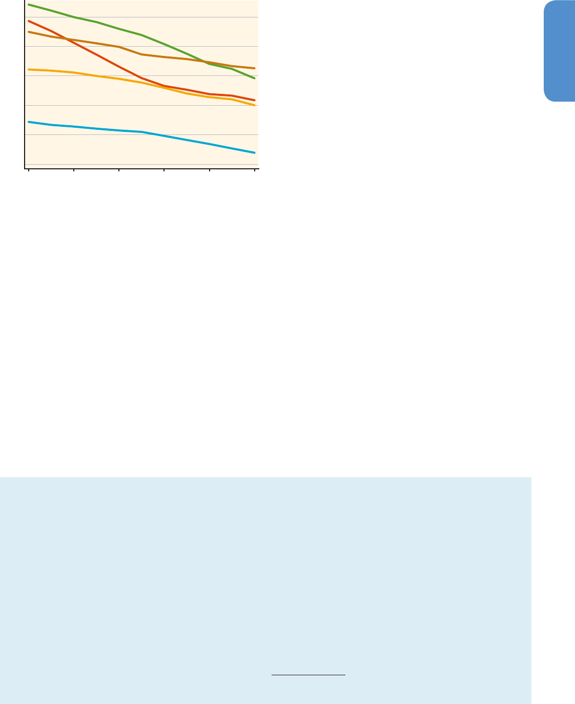
393393
Drivers, Trends and Mitigation
5
Chapter 5
health and environmental benefits) before focusing on climate policy
(Nemet etal., 2010b; Klimont etal., 2013). If this is indeed the case,
the co-benefits of climate policy will be much smaller. Figure 5.22
shows the declining trend in SO
2
-emission intensity per CO
2
emissions
(see Section 5.2 for trends in global SO
2
emissions). It shows that
assumptions about the extrapolation of the historic trends into the
future will be a major determinant of future co-benefits estimates
(Burtraw and Evans, 2003; Bell etal., 2008), see Section 6.6.2.7 for an
example from the scenario literature).
Due to a lack of a counterfactual historic baseline for other policies, it
is not possible to determine a clean ex-post measure for the co-ben-
efits of climate policies such as the Kyoto Protocol. But it is clear that
drivers for fossil fuel combustion affect both CO
2
emissions and SO
2
emissions (see van Vuuren etal., 2006).
5�7�2 Adverse side-effects
There are also adverse side-effects associated with mitigation. A com-
prehensive discussion is given in the following chapters (6 – 12), while
this section presents some examples in the context of air pollution.
While many low-carbon energy supply technologies perform better
than pulverized coal technologies for most air pollutants, some solar
energy technologies, for example, have comparable or even higher
life-cycle emissions of SO
2
(see Figure 7.8 in Section 7.9.2). Desul-
phurization of existing coal power plants, however, requires additional
consumption of coal in the thermal power sector implying higher CO
2
emissions for a given electricity output (Pan, 2013). While CO
2
capture
processes reduce SO
2
emissions at the same time, some carbon diox-
ide capture and storage (CCS) technologies would imply an increase in
NO
x
and / or ammonia (NH
3
) emissions (Koornneef etal., 2012).
For the displacement of fossil-based transport fuels with biofuels,
many studies indicate lower carbon monoxide and hydrocarbon emis-
sions, but NO
x
emissions are often higher. Next-generation biofuels are
expected to improve performance, such as the low particulate matter
emissions from lignocellulosic ethanol (see Hill etal., 2009; Sathaye
etal., 2011; and Sections 8.7 and 11. A.6). In the buildings sector, the
most important health risks derive from insufficient ventilation prac-
tices in air-tight buildings (Section 9.7).
5�7�3 Complex issues in using co-benefits and
adverse side-effects to inform policy
Mitigation options that improve productivity of energy, water, or land
use yield, in general, positive benefits. The impact of other mitigation
actions depend on a wider socio-economic context within which the
action is implemented (Sathaye etal., 2007). A complete incorporation
of co-benefits and adverse side-effects into climate policy is compli-
Box 5�5 | The Chinese experience with co-benefits from a cross-sectoral perspective
1
Pan etal. (Pan etal., 2011) estimate the amount of green jobs in
three sectors (energy, transportation, and forestry) and the result
suggests a number at least 4.5 million in 2020 in China. The wind
power industry in China, including power generation and turbine
manufacturing, has created 40,000 direct jobs annually between
2006 and 2010 (Pan etal., 2011). Beijing’s ambitious metro-
system plan, which includes 660 km by 2015 and another 340
km during 2016 – 2020,could bring more than 437,000 jobs each
year (Pan etal., 2011). China’s forestation activities could create
as many as 1.1million direct and indirect jobs annually during
2011 – 2020 to achieve its 2020 goals (Pan etal., 2011).
In 2007, China called for a more environmentally friendly and
resource-saving models of production and consumption (Pan,
2012). Twelve out of 17 mandatory targets in the 12th five-
year (2011 – 2015) plan are related to the protection of natural
resources and the environment; the rest are related to the
improvement of social welfare (Pan, 2012). The actions taken
under the five-year plan include progressive pricing for electric-
ity consumption; implementation of energy consumption quota,
disaggregated emission targets; emissions-trading schemes; initia-
tives for eco-cities and low-carbon cities; and upgraded building
codes with improved enforcement (Pan, 2012).
1
See Sections 7.9, 8.7, 9.7, 10.9, and 11.8 for sectoral effects.
5�7�1 Co-benefits
A substantial share of estimated co-benefits is related to improving
health through limiting air pollution while reducing GHG emissions.
Estimates in the literature for the monetized air quality co-benefits
from climate change mitigation range from 2 to 930 USD
2010
/ tCO
2
, and
co-benefits in developing countries around twice those in industrialized
countries (see Nemet etal., 2010a) for a review and (West etal., 2013)
for the high estimate. The gap between developing and industrialized
countries results from lower levels of air pollution control and higher
pollution levels in the former countries, and thus the greater potential
for improving health, particularly in the transport and household energy
demand sectors (Markandya et al., 2009; Nemet etal., 2010b; West
etal., 2013; Shukla and Dhar, 2011). In industrialized countries, sub-
stantial reductions in air pollutant emissions have already occurred in
the absence of climate policy and further tightening of air regulations is
underway (Rao etal., 2013). If climate policy provides only small incre-
mental reductions, then the co-benefit is small (see Section 3.6.3),
while large emission reductions are expected to yield substantial air
quality co-benefits and associated cost savings (see Section 6.6.2).
Much of the literature assessed in AR4 did not explicitly analyze poli-
cies targeted at reducing air pollution−thereby neglecting the associ-
ated opportunity costs of mitigation polices (Bollen etal., 2009; Eden-
hofer etal., 2013). But for countries and regions that do not have or do
not enforce current air quality regulations, it is important to consider
expected future air pollution policies. Rapidly industrializing develop-
ing countries may follow the pattern of developed countries and adopt
regulations to improve local air quality (and provide immediate local
Figure 5�22 | Trends for SO
2
per CO
2
emissions per region over 2000 – 2010 | For CO
2
:
territorial, excluding AFOLU and Waste. Data Source: JRC / PBL, 2013. For SO
2
, data
source: Klimont etal., 2013. Regions are defined in Annex II.2.
2000 2002 2004 2006 2008 2010
Asia
Latin America
Middle East and Africa
OECD-1990 Countries
Economies in Transition
1
2
3
4
5
6
SO
2
/CO
2
Emissions [kgSO
2
/tCO
2
]

394394
Drivers, Trends and Mitigation
5
Chapter 5
cated, but it is part of a shift of the development paradigm towards
sustainability (Pan, 2012).
Co-benefits are pervasive and inseparable (Grubb etal., 2013). It is
not possible to ‘separate’ each benefit with different decisions: both
technically and politically, most decisions involve multiple dimensions.
In addition, most suggested policy changes involve large changes
in the policy environment as opposed to the concept of marginal
changes (see also Section 3.6.3). Finally, many effects are measured
in very different metrics or are not quantified at all. As an example,
whereas local air quality co-benefits are measured in health terms,
energy security is typically measured with indicators of the sufficiency
of domestic resources (e. g., dependence on fossil fuel imports) and
resilience of energy supply (see Sections 6.6 and 7.9 for details). All
these characteristics make a comprehensive analysis of co-benefits
and adverse side-effects of a particular policy or measure challenging.
This is why a synthesis of results from different research communities
is crucial for robust decision making (see Section 6.6).
Despite the difficulties, side-effects from climate policy are important
for policy design (see Section15.2.4). Costs of mitigation policies are
over- or under-estimated when co-benefits and adverse side-effects are
not included (see Sections 3.6.3 and 6.3.6). Co-benefits estimates are
particularly important for policymakers because most of the climate
benefits are realized decades into the future while most co-benefits,
such as improvement in air quality, are realized immediately (Barker
etal., 2008; Nemet etal., 2010b; Shindell etal., 2012; Jack and Kinney,
2010; Henriksen etal., 2011).
5.8 The system perspective:
linking sectors,
technologies and
consumption patterns
Between 1970 and 2010 global greenhouse gas emissions have
increased by approximately 80 %. The use of fossil fuels for energy
purposes has been the major contributor to GHG emissions. Emissions
growth can be decomposed in population growth and per capita emis-
sions growth. Population growth is a major immediate driver for global
GHG-emissions trends. Global population grew from 3.7 to 6.9 billion.
The largest growth rates are found in MAF.
GHG emissions can be attributed to regions according to the territo-
rial location of emissions, or alternatively emissions can be attributed
to the consumption of goods and services, and located to regions
where consumption takes place. There is an emerging gap between
territorial and consumption-based emissions, signalling a trend where
a considerable share of CO
2
emissions from fossil fuel combustion in
developing countries is released in the production of goods and ser-
vices exported to developed countries. At a regional level, OECD-1990
is the largest net importer of CO
2
embedded in trade, while ASIA is
the largest net exporter. This emerging gap opens questions about the
apparent decoupling between economic growth and GHG emissions
in several Annex I countries; when consumption-related emissions are
taking into account both GDP and GHG emissions have grown. Yet, a
robust result is that, between 2000 and 2010, the developing country
group has overtaken the developed country group in terms of annual
CO
2
emissions from fossil fuel combustion and industrial processes,
from both territorial and consumption perspectives.
When considering per capita emissions, rather than aggregate GHG
emissions, other trends become visible. Global average per capita GHG
emissions have shown a rather stable trend over the last 40 years.
This global average, however, masks differences between regions and
sectors. A strong correlation appears between per capita income and
per capita GHG emissions both from a cross-country comparison on
income and emission levels, and when considering income and emis-
sions growth. The relation is most clearly for the sectors’ energy,
industry, and transport (Section 5.3.5), and holds despite the reduc-
tion in the average emission intensity of production, from 1.5 to
0.73kgCO
2
eq / Int$
2005
over the same 40-year period.
ASIA had low per capita emission levels in 1970, but these increased
steadily, by more than 150 %. The EIT region showed a rapid increase in
per capita emissions between 1970 and 1990, and a sharp drop imme-
diately after 1990. In 2010, per capita emissions are comparable in
ASIA, LAM, and MAF (5.2, 6.4, and 5.4 tCO
2
eq / yr, respectively) but per
capita GHG emissions in OECD-1990 and EIT are still higher by a factor
of 2 to 3 (14.1 and 11.9 tCO
2
eq / yr, respectively). Also, between 1970
and 2010, per capita land-use related emissions decreased, but fossil
fuel-related emissions increased. Regions vary greatly with respect to
the income trends. The OECD-1990 and LAM countries showed a stable
growth in per capita income, which was in the same order of magni-
tude as the GHG-intensity improvements, so that per capita emissions
remained almost constant and total emissions increased by the rate of
population growth. The EIT showed a decrease in income around 1990,
which together with decreasing emissions per output and a very low
population growth led to a robust decrease in overall emissions. The
MAF sector also shows a decrease in GDP per capita but a high popu-
lation growth led to a robust increase in overall emissions. Emerging
economies in Asia showed very high economic growth rates; rapidly
expanding industries resulted in sharply increasing emissions. In 2010,
ASIA emitted more than half of worldwide industry-related emissions.
ASIA showed both the highest economy-wide efficiency improvements
measured as output per emissions, and the largest growth in per capita
emissions.
The underlying drivers for economic growth are diverse and vary
among regions and countries. Technological change and human capital
are key underlying drivers, but some authors also underscore the avail-
ability of energy resources to play a central role in economic growth.
Economic growth is strongly correlated to growth in energy use, and

395395
Drivers, Trends and Mitigation
5
Chapter 5
the direction of causality is not clearly established. At the global level,
per capita primary energy consumption rose by 29 % from 1970 to
2010, but due to population growth total energy use has increased
much more−140 % over the same period.
Energy-related GHG emissions can be further decomposed in two addi-
tional immediate drivers: energy intensity and carbon intensity. Energy
intensity has declined globally in all developed and major develop-
ing countries including India and China. This decline can be explained
through technological changes, the effects of structural changes, and
the substitution of other inputs such as capital and labour used. These
historical improvements in energy intensities, however, have not been
enough to compensate the effect of GDP growth, thus, increasing
energy consumption over time as a result.
In addition, energy resources have historically become less carbon-
intensive, though increased use of coal, relative to other resources,
since 2000 has changed the trends exacerbating the burden of energy-
related GHG emissions. Estimates of the resources of coal and conven-
tional plus unconventional gas and oil are very large; indicating that
resource scarcity has not been and will not be an underlying driver for
decarbonization.
The immediate drivers that directly affect GHG emissions, namely
population, GDP per capita, energy intensity and carbon intensity, are
affected, in turn, by underlying drivers as described in Figure 5.1. These
underlying drivers include resource availability, development status
and goals, level of industrialization and infrastructure, international
trade, urbanization, technological changes, and behavioural choices.
Among these, infrastructure, technological changes and behavioural
choices appear to be critical but, even though their influences on other
drivers is well established, the magnitude of this impact remains dif-
ficult to quantify.
Co-benefits have large potential to contribute to emission reductions,
but its historic contribution is not established. Infrastructural choices
have long-lasting effects directing the development path to higher
or lower energy and carbon intensities. Infrastructure also guides the
choices in technological innovation. Technological change affects both
income and emission intensity of income; it can lead to both increasing
and decreasing GHG emissions. Historically, innovation increased income
but also resource use, as past technological change has favoured labour
productivity increase over resource efficiency. There is clear empirical
evidence that prices and regulation affect the direction of innovations.
Innovations that increase energy efficiency of appliances often also lead
to increased use of these appliances, diminishing the potential gains
from increased efficiency, a process called ‘rebound effect’.
Behaviour and life-styles are important underlying drivers affecting the
emission intensity of expenditures through consumption choices and
patterns for transportation modes, housing, and food. Behaviour and
lifestyles are very diverse, rooted in individuals' psychological traits,
cultural, and social context, and values that influence priorities and
actions concerning climate change mitigation. Environmental values
are found to be important for the support of climate change policies
and measures. Chapter 4 discusses formal and civil institutions and
governance in the context of incentivizing behavioural change. There
are many empirical studies based on experiments showing behavioural
interventions to be effective as an instrument in emission reductions,
but not much is known about the feasibility of scaling up experiments
to the macro economy level.
As described across the different sections of the chapter, factors and
drivers are interconnected and influence each other and, many times,
the effects of an individual driver on past GHG emissions are difficult
to quantify. Yet historic trends reveal some clear correlations. Histori-
cally, population growth and per capita income growth have been
associated with increasing energy use and emissions. Technological
change is capable to substantially reduce emissions, but historically,
labour productivity has increased more compared to resource produc-
tivity leading to increased emissions. Regulations and prices are estab-
lished as directing technological change towards lower emission inten-
sities. Behavioural change is also established as a potentially powerful
underlying driver, but not tested at the macro level. Policies and mea-
sures can be designed and implemented to affect drivers but at the
same time these drivers influence the type of policies and measures
finally adopted. Historic policies and measures have proved insufficient
to curb the upward GHG emissions trends in most countries. Future
policies need to provide more support for emission reductions com-
pared to policies over the period 1970 – 2010, if the aim is to change
the future GHG emissions trends.
5.9 Gaps in knowledge
and data
• There is a need for a more timely and transparent update
of emission estimates� The collection and processing of statistics
of territorial emissions for almost all countries since 1970, as used
in Section 5.2, is far from straightforward. There are multiple data
sources, which rarely have well-characterized uncertainties. Uncer-
tainty is particularly large for sources without a simple relationship
to activity factors, such as emissions from LUC, fugitive emissions,
and gas flaring. Formally estimating uncertainty for LUC emissions
is difficult because a number of relevant processes are not well-
enough characterized to be included in estimates. Additionally, the
dependence of the attribution of emissions to sectors and regions
on the relative weight given to various GHGs is often not specified.
• The calculation of consumption-based emissions (in addition
to territorial emissions) is dependent on strong assumptions�
The calculations require an additional layer of processing on top of
the territorial emissions, increasing uncertainties without a clear

396396
Drivers, Trends and Mitigation
5
Chapter 5
characterization of the uncertainties. The outcomes presented in
Sections 5.3.1 and 5.3.3.2 are only available for years since 1990.
• Empirical studies that connect GHG emissions to specific
policies and measures or underlying drivers often cannot be
interpreted in terms of causality, have attribution problems,
and provide competing assessments� Statistical association
is not the same as a chain of causality, and there are competing
explanations for correlations. Studies can attribute changes in
emissions to changes of activities when all other things are kept
equal, but historically, all other things rarely are equal. Section 5.3
identifies population, income, the economic structure, the choice of
energy sources related to energy resource availability and energy
price policies as proximate and underlying drivers for greenhouse
gas emissions. But for most demography variables other than the
population level, the literature provides competing assessments;
different studies find different significant associations, and at dif-
ferent levels. Underlying drivers work in concert and cannot be
assessed independently. From a cause-effect perspective, there
is, for instance, no conclusive answer whether ageing, urbaniza-
tion, and increasing population density as such lead to increasing
or decreasing emissions; this depends on other underlying drivers
as well. The results from the literature are often limited to a spe-
cific context and method. Our understanding could benefit from a
rigorous methodological comparison of different findings (Sections
5.3.2, 5.6, 5.7).
• It is debated whether greenhouse gas emissions have an
‘autonomous’ tendency to stabilize at higher income lev-
els (Section 5.3.3.1). It is agreed that economic growth increases
emissions at low- and middle-income levels. With respect to
energy, there are competing views whether energy availability is
a driver for economic growth, or inversely that economic growth
jointly with energy prices drives energy use, or that the causality
depends on the stage of development (Sections 5.3.3.1 and 5.3.4).
• The net effect of trade, behaviour, and technological change
as a determinant of a global increase or decrease of emis-
sions is not established (Sections 5.4.2, 5.6.1, 5.7). There is
evidence that the social, cultural, and behavioural context is an
important underlying driver, and there are case studies that iden-
tify emission reductions for specific policies and technologies. For
technology, empirical studies that ask whether innovations have
been emission-saving or emission-increasing are limited in scope
(Section 5.6.1). There is a rich theory literature on the potential
of innovations to make production energy — or emission effi-
cient — but evidence on the macro-effects and the rebound effect
is still context-dependent (Section 5.6.2). How much carbon is
exactly locked in existing physical infrastructure is uncertain and
gaps of knowledge exist in how long physical infrastructure like
housing, plants, and transport infrastructure typically remains in
place in which geographical context (Section 5.6.3). Finally, most if
not all of the literature on co-benefits and risk tradeoffs focuses on
future potential gains. There is a total absence of empirical assess-
ment about the role that co-benefits and adverse sideeffects have
played, historically, in policy formation and GHG emissions (Sec-
tion5.7).
5.10 Frequently Asked
Questions
FAQ 5�1 Based on trends in the recent past, are
GHG emissions expected to continue to
increase in the future, and if so, at what
rate and why?
Past trends suggest that GHG emissions are likely to continue to
increase. The exact rate of increase cannot be known but between 1970
and 2010, emissions increased 79 %, from 27Gt of GHG to over 49Gt
(Figure 5.2). Business-as-usual would result in that rate continuing.
The UN DESA World Population Division expects human population to
increase at approximately the rate of recent decades (Section 5.3.2.1)
of this report. The global economy is expected to continue to grow
(Sections 5.3.3 and 5.4.1), as well as energy consumption per person
(Sections 5.3.4.1 and 5.5.1). The latter two factors already vary greatly
among countries (Figure 5.16), and national policies can affect future
trajectories of GHG emissions directly as well as indirectly through
policies affecting economic growth and (energy) consumption (Section
5.5). The existing variation and sensitivity to future policy choices make
it impossible to predict the rate of increase in GHG emissions accu-
rately, but past societal choices indicate that with projected economic
and population growth, emissions will continue to grow (Section 5.8).
FAQ 5�2 Why is it so hard to attribute causation
to the factors and underlying drivers
influencing GHG emissions?
Factors influencing GHG emissions interact with each other directly
and indirectly, and each factor has several aspects. Most things people
produce, consume, or do for recreation result in GHG emissions (Sec-
tions 5.3 and 5.5). For example, the food chain involves land use, infra-
structure, transportation, and energy production systems (Section 5.3).
At each stage, emissions can be influenced by available agricultural
and fishing technologies (Section 5.6), by intermediaries along the
supply chain (Section 5.4), by consumers and by technology choices
(Section 5.5). Technology and choice are not independent: available
technologies affect prices, prices affect consumer preferences, and con-
sumer preferences can influence the development and distribution of
technologies (Sections 5.5). Policies, culture, traditions, and economic
factors intervene at every stage. The interaction of these factors makes
it difficult to isolate their individual contributions to carbon emissions

397397
Drivers, Trends and Mitigation
5
Chapter 5
growth or mitigation (Section 5.8). This interaction is both a cause for
optimism, because it means there are many pathways to lower emis-
sions, and a challenge because there will be many potential points of
failure in even well-designed plans for mitigation.
FAQ 5�3 What options, policies, and measures
change the trajectory of GHG emissions?
The basic options are to have individuals consume less, consume things
that require less energy, use energy sources that have lower-carbon
content, or have fewer people. Although inhabitants of the most devel-
oped countries have the option to consume less, most of the human
population is located in less-developed countries and economies in
transition where population growth is also higher (Section 5.3.2). In
these countries, achieving a ‘middle-class lifestyle’ will involve con-
suming more rather than less (Section 5.3.3.2). Accepting that popula-
tion will continue to grow, choices will involve changes in technology
and human behaviour, so that the production and use of products and
services is associated with lower rates of GHG emissions (technology
Section 5.6), and consumers choose products, services, and activities
with lower-unit GHG emissions (behaviour Section 5.5).
FAQ 5�4 What considerations constrain the range
of choices available to society and their
willingness or ability to make choices
that would contribute to lower GHG
emissions?
Choices are constrained by what is available, what is affordable, and
what is preferred (Section 5.3.3). For a given product or service, less
carbon-intensive means of provision need to be available, priced
accessibly, and appeal to consumers (Section 5.3.4.2). Availability is
constrained by infrastructure and technology, with a need for options
that are energy-efficient and less-dependent on fossil fuels (Section
5.3.5). The choice of what to consume given the availability of acces-
sible and affordable options is constrained by preferences due to cul-
ture, awareness, and understanding of the consequences in terms of
emissions reduction (Sections 5.5.1, 5.5.2). All of these constraints can
be eased by the development of alternative energy generation tech-
nologies and distribution systems (Section 5.6), and societies that are
well-informed about the consequences of their choices and motivated
to choose products, services, and activities that will reduce GHG emis-
sions (Sections 5.5.3, 5.7).

398398
Drivers, Trends and Mitigation
5
Chapter 5
References
Abrahamse W�, L� Steg, C� Vlek, and T� Rothengatter (2005)� A review of inter-
vention studies aimed at household energy conservation. Journal of Environ-
mental Psychology 25, 273 – 291.
Ackerman F�, M� Ishikawa, and M� Suga (2007)� The carbon content of Japan-US
trade. Energy Policy 35, 4455 – 4462.
Ackerman K� V�, and E� T� Sundquist (2008)� Comparison of two US power-plant
carbon dioxide emissions data sets. Environmental Science & Technology 42,
5688 – 5693. doi: 10.1021 / Es800221q, ISSN: 0013-936X.
Aghion P�, A� Dechezleprêtre, D� Hemous, R� Martin, and J� Van Reenen (2012)�
Carbon Taxes, Path Dependency and Directed Technical Change: Evidence from
the Auto Industry. London, UK, 76 pp.
Aghion P�, and P� Howitt (2009)� The Economics of Growth. MIT Press, Cambridge
Mass. ISBN: 9780262012638.
Aichele R�, and G� Felbermayr (2012)� Kyoto and the carbon footprint of nations.
J. Environmental Economics and Management 63, 336 – 354.
Aichele R�, and G� Felbermayr (2013)� Estimating the effects of Kyoto on bilat-
eral trade flows using matching econometrics. The World Economy. doi:
0.1111 / twec.12053.
Akerlof G� A� (1970)� The market for “lemons”: Quality uncertainty and the
market mechanism. The Quarterly Journal of Economics 84, 488 – 500. doi:
10.2307 / 1879431, ISSN: 00335533.
Alam S� S�, A� Khatibi, M� I� S� Ahmad, and H� B� Ismail (2008)� Factors affecting
e-commerce adoption in the electronic manufacturing companies in Malay-
sia. International Journal of Commerce and Management 17, 125 – 139. doi:
10.1108 / 10569210710776503, ISSN: 1056-9219.
Allcott H� (2011)� Social norms and energy conservation. Journal of Public Econom-
ics 95, 1082 – 1095. doi: 10.1016 / j.jpubeco.2011.03.003, ISSN: 0047-2727.
Allcott H�, and M� Greenstone (2012)� Is There an Energy Efficiency Gap?
National Bureau of Economic Research, Available at: http: / / www. nber.
org / papers / w17766.
Allen R� (2009)� The British Industrial Revolution in Global Perspective. Cambridge
Univ. Press, Cambridge [u. a.], ISBN: 9780521687850.
Ameli N�, and D� M� Kammen (2012)� Clean energy deployment: addressing
financing cost. Environmental Research Letters 7, 034008. doi: 10.1088 / 1748-
9326 / 7 / 3 / 034008, ISSN: 1748-9326.
Andres R� J�, T� A� Boden, F�-M� Bréon, P� Ciais, S� Davis, D� Erickson, J� S� Gregg,
A� Jacobson, G� Marland, J� Miller, T� Oda, J� G� J� Olivier, M� R� Raupach, P�
Rayner, and K� Treanton (2012)� A synthesis of carbon dioxide emissions from
fossil-fuel combustion. Biogeosciences 9, 1845 – 1871. doi: 10.5194 / bg-9-1845-
2012, ISSN: 1726-4189.
Andrew R� M�, and G� P� Peters (2013)� A multi-region input – output table based
on the global trade analysis project database (gtap-Mrio). Economic Systems
Research 25, 99 – 121. doi: 10.1080 / 09535314.2012.761953, ISSN: 0953-5314.
Ang B� W� (2006)� Monitoring changes in economy-wide energy efficiency: From
energy-GDP ratio to composite efficiency index. Energy Policy 34, 574 – 582.
doi: 16 / j.enpol.2005.11.011, ISSN: 0301-4215.
Angel D� P�, S� Attoh, D� Kromm, J� Dehart, R� Slocum, and S� White (1998)� The
drivers of greenhouse gas emissions: what do we learn from local case studies?
Local Environment 3, 263 – 277.
Arrow et al K� (1996)� Economic growth, carrying capacity, and the environment.
Ecological Applications 6, 13 – 15. Available at: http: / / www. jstor. org / stable /
2269539.
Axelrod R� (2006)� Robert Axelrod. 1986. An evolutionary approach to norms.
American Political Science Review 80 (December): 1095 – 1111. The American
Political Science Review 100, 682 – 683. doi: 10.2307 / 27644412, ISSN: 0003-
0554.
Ayres I�, S� Raseman, and A� Shih (2009)� Evidence from Two Large Field
Experiments That Peer Comparison Feedback Can Reduce Residential Energy
Usage. National Bureau of Economic Research, Cambridge, MA. Available at:
http: / / www. nber. org / papers / w15386.
Ayres R�, and B� Warr (2009)� The Economic Growth Engine: How Energy
and Work Drive Material Prosperity. Edward Elgar, Cheltenham, UK, ISBN:
9781848441828.
Azar C�, and H� Dowlatabadi (1999)� A review of technical change in assessment
of climate policy. Annual Review of Energy and the Environment 24, 513 – 544.
doi: 10.1146 / annurev.energy.24.1.513, ISSN: 1056-3466, 1056 – 3466.
Babiker M� H� (2005)� Climate change policy, market structure, and carbon leak-
age. Journal of International Economics 65, 421 – 445. Available at: http: / / ideas.
repec.org / a / eee / inecon / v65y2005i2p421-445.html.
De Backer K�, and N� Yamano (2012)� International Comparative Evidence on
Global Value Chains. Organisation for Economic Co-Operation and Develop-
ment, Paris. Available at: http: / / www. oecd-ilibrary. org / content / workingpaper /
5k9bb2vcwv5j-en.
Backer K� D�, and N� Yamano (2007)� The Measurement of Globalisation Using
International Input-Output Tables. OECD Publishing. Available at: http: / / ideas.
repec.org / p / oec / stiaaa / 2007-8-en.html.
Baiocchi G�, and J� C� Minx (2010)� Understanding changes in the UK’s CO
2
emissions: A global perspective. Environmental Science & Technology 44,
1177 – 1184. doi: 10.1021 / es902662h, ISSN: 0013-936X.
Ballantyne A� P�, C� B� Alden, J� B� Miller, P� P� Tans, and J� W� C� White (2012)�
Increase in observed net carbon dioxide uptake by land and oceans during the
past 50 years. Nature 488, 70 – 72. doi: 10.1038 / nature11299, ISSN: 0028-0836.
Ballantyne A� P�, D� R� Greenwood, J� S� S� Damsté, A� Z� Csank, J� J� Eberle, and
N� Rybczynski (2010)� Significantly warmer Arctic surface temperatures during
the Pliocene indicated by multiple independent proxies. Geology 38, 603 – 606.
doi: 10.1130 / G30815.1, ISSN: 0091-7613, 1943 – 2682.
Ballesteros A�, S� Nakhooda, J� Werksman, and K� Hurlburt (2010)� Power,
responsibility, and accountability: Rethinking the legitimacy of institutions for
climate finance. Climate Law 1, 261 – 312. doi: 10.3233 / CL-2010-013.
Banister D� (2011a)� The trilogy of distance, speed and time. Journal of Transport
Geography 19, 950 – 959. doi: 10.1016 / j.jtrangeo.2010.12.004, ISSN: 0966-
6923.
Banister D� (2011b)� Cities, mobility and climate change. Journal of Transport
Geography 19, 1538 – 1546. doi: 10.1016 / j.jtrangeo.2011.03.009, ISSN: 0966-
6923.
Banister D�, and M� Thurstain-Goodwin (2011)� Quantification of the non-trans-
port benefits resulting from rail investment. Journal of Transport Geography 19,
212 – 223. doi: 10.1016 / j.jtrangeo.2010.05.001, ISSN: 0966-6923.

399399
Drivers, Trends and Mitigation
5
Chapter 5
Barker T�, A� Alharthi, M� Amann, L� Cifuentes, J� Drexhage, R� Duan, O� Eden-
hofer, B� Flannery, M� Grubb, M� Hoogwijk, F� I� Ibitoye, C� J� Jepma, W� A�
Pizer, and K� Yamaji (2008)� Mitigation from a cross-sectoral perspective. In:
Climate Change 2007: Mitigation. Contribution of Working Group III to the
Fourth Assessment Report of the Intergovernmental Panel on Climate Change.
B. Metz, O. R. Davidson, P. R. Bosch, R. Dave, L. A. Meyer (eds.), Cambridge Uni-
versity Press, Cambridge, United Kingdom.
Barker T�, P� Ekins, and T� Foxon (2007)� The macro-economic rebound
effect and the UK economy. Energy Policy 35, 4935 – 4946. doi: 10.1016 / j.
enpol.2007.04.009, ISSN: 0301-4215.
Barrett J�, K� Roelich, T� Wiedmann, J� Minx, and A� Owen (2013)� Learning from
the past, evaluating futures? Sustainable consumption and production evi-
dence and applications in the UK. Environment and Planning.
Becker L� J�, C� Seligman, R� H� Fazio, and J� M� Darley (1981)� Relating atti-
tudes to residential energy use. Environment and Behavior 13, 590 – 609. doi:
10.1177 / 0013916581135004, ISSN: 0013-9165, 1552 – 390X.
Bednar-Friedl B�, T� Schinko, and K� W� Steininger (2012)� The relevance of pro-
cess emissions for carbon leakage: A comparison of unilateral climate policy
options with and without border carbon adjustment. Energy Economics 34,
Supplement 2, 168 – 180. doi: 10.1016 / j.eneco.2012.08.038, ISSN: 0140-9883.
Bell M� L�, D� L� Davis, L� A� Cifuentes, A� J� Krupnick, R� D� Morgenstern, and
G� D� Thurston (2008)� Ancillary human health benefits of improved air qual-
ity resulting from climate change mitigation. Environmental Health 7, 41. doi:
10.1186 / 1476-069X-7-41, ISSN: 1476-069X.
Bentzen J� (2004)� Estimating the rebound effect in US manufacturing energy
consumption. Energy Economics 26, 123 – 134. doi: 10.1016 / S0140-
9883(03)00047-1, ISSN: 0140-9883.
Van den Bergh J� C� J� M� (2010)� Energy conservation more effective with
rebound policy. Environmental and Resource Economics 48, 43 – 58. doi:
10.1007 / s10640-010-9396-z, ISSN: 0924-6460.
Van den Bergh J� C� J� (2008)� Environmental regulation of households: An empiri-
cal review of economic and psychological factors. Ecological Economics 66,
559 – 574.
Berkhout P� H� G�, J� C� Muskens, and J� W� Velthuijsen (2000)� Defin-
ing the rebound effect. Energy Policy 28, 425 – 432. doi: 10.1016 / S0301-
4215(00)00022-7, ISSN: 0301-4215.
Biel A�, and L� J� J� Lundqvist (2012)� From Kyoto to the Town Hall: Making Interna-
tional and National Climate Policy Work at the Local Level. Routledge (Oxford,
UK), 152 pp. ISBN: 9781136565182.
Black C�, A� Collins, and M� Snell (2001)� Encouraging walking: The case of jour-
ney-to-school trips in compact urban areas. Urban Studies 38, 1121 – 1141. doi:
10.1080 / 00420980124102, ISSN: 0042-0980, 1360 – 063X.
Blodgett J�, and L� Parker (2010)� Greenhouse Gas Emission Drivers: Population,
Economic Development and Growth, and Energy Use. Congressional Report
Service, Washington, D. C. Available at: http: / / www. cnie. org / NLE / CRSreports /
10Apr / RL33970.pdf.
Blundell R�, R� Griffith, and J� van Reenen (1999)� Market share, market value
and innovation in a panel of British manufacturing firms. Review of Economic
Studies 66, 529 – 554.
Boden T� A�, G� Marland, and R� J� Andres (2012)� Global, Regional, and National
Fossil-Fuel CO
2
Emissions. Carbon Dioxide Information Analysis Center, Oak
Ridge National Laboratory, U. S. Department of Energy, Oak Ridge, Tenn., U. S. A.
Boehringer C�, T� Rutherford, and E� Balistreri (2012)� The role of border carbon
adjustment in unilateral climate policy, insights from an EMF model compari-
son. Energy Economics.
Bogner J�, R� Pipatti, S� Hashimoto, C� Diaz, K� Mareckova, L� Diaz, P� Kjeldsen,
S� Monni, A� Faaij, Q� Gao, T� Zhang, M� A� Ahmed, R� T� M� Sutamihardja,
and R� Gregory (2008)� Mitigation of global greenhouse gas emissions from
waste: conclusions and strategies from the Intergovernmental Panel on Cli-
mate Change (IPCC) Fourth Assessment Report. Working Group III (Mitigation).
Waste Management & Research 26, 11 – 32. doi: 10.1177 / 0734242X07088433,
ISSN: 0734-242X, 1096 – 3669.
Bolla V�, and V� Pendolovska (2011)� Driving Forces Behind EU-27 Greenhouse
Gas Emissions over the Decade 1999 – 2008. Eurostat. Available at: http: / / epp.
eurostat.ec.europa.eu / cache / ITY_OFFPUB / KS-SF-11-010 / EN / KS-SF-11-010-EN.
PDF.
Bollen J�, B� Guay, S� Jamet, and J� Corfee-Morlot (2009)� Co-Benefits of Climate
Change Mitigation Policies: Literature Review and New Results. OECD Publish-
ing, Paris, France. Available at: http: / / ideas.repec.org / p / oec / ecoaaa / 693-en.
html.
Bond T� C�, E� Bhardwaj, R� Dong, R� Jogani, S� K� Jung, C� Roden, D� G� Streets,
and N� M� Trautmann (2007)� Historical emissions of black and organic carbon
aerosol from energy-related combustion, 1850 – 2000. Global Biogeochemical
Cycles 21. doi: 10.1029 / 2006gb002840, ISSN: 0886-6236.
Bond T� C�, S� J� Doherty, D� W� Fahey, P� M� Forster, T� Berntsen, B� J� DeAngelo,
M� G� Flanner, S� Ghan, B� Karcher, D� Koch, S� Kinne, Y� Kondou, P� K� Quinn,
M� C� Sarofim, M� G� Schultz, C� Venkataraman, H� Zhang, S� Zhang, N� Bell-
ouin, S� K� Guttikunda, P� K� Hopke, M� Z� Jacobson, J� W� Kaiser, Z� Klimont,
U� Lohmann, J� P� Schwarz, D� Shindell, T� Storelvmo, S� G� Warren, and C� S�
Zender (2013)� Bounding the role of black carbon in the climate system: A
scientific assessment. Journal of Geophysical Research 118, 5380 – 5552.
Bond T� C�, D� G� Streets, K� F� Yarber, S� M� Nelson, J�-H� Woo, and Z� Klimont
(2004)� A technology-based global inventory of black and organic carbon emis-
sions from combustion. Journal of Geophysical Research 109, D14203.
Bosetti V�, and E� Verdolini (2012)� Heterogeneous Firms Trading In Ideas: An
Application to Energy Technologies. Available at: http: / / graduateinstitute.
ch / files / live / sites / iheid / files / sites / cies / shared / publications / InnovationWork-
shop / VB_EV_Heterogenous_Geneva.pdf.
Boucher O�, and D� Randall (2013)� Chapter 7: Clouds and Aerosols. In: Climate
Change 2013: The Physical Science Basis. Contribution of Working Group I to
the Fifth Assessment Report of the Intergovernmental Panel on Climate Change
[T. F. Stocker, D. Qin, G.-K. Plattner, M. Tignor, S. K. Allen, J. Boschung, A. Nauels,
Y. 40 Xia, V. Bex, P. M. Midgley, (eds.)]. Cambridge University Press, Cambridge,
UK and New York, NY USA.
BP (2013)� BP Statistical Review of World Energy. British Petroleum, UK. Available at:
http: / / www. bp. com / content / dam / bp / pdf / statistical-review / statistical_review_
of_world_energy_2013.pdf.
Brock W�, and M� Taylor (2010)� The Green Solow model. Journal of Economic
Growth 15, 127 – 153. doi: 10.1007 / s10887-010-9051-0, ISSN: 1381-4338.
Bruckner T�, O� Edenhofer, H� S� Matthews, M� Haller, M� Lüken, N� Bauer, and
N� Nakicenovic (2010)� Robust options for decarbonization. In: Global Sus-
tainability: A Nobel Cause. H.-J. Schellnhuber, M. Molina, N. Stern, V. Huber, S.
Kadner (eds.), Cambridge University Press, pp. 189 – 204.

400400
Drivers, Trends and Mitigation
5
Chapter 5
Bryan J� E�, P� L� Shearman, G� P� Asner, D� E� Knapp, G� Aoro, and B� Lokes
(2013)� Extreme differences in forest degradation in Borneo: comparing prac-
tices in Sarawak, Sabah, and Brunei. PloS One 8, e69679. doi: 10.1371 / journal.
pone.0069679, ISSN: 1932-6203.
Burtraw D�, and D� Evans (2003)� The Evolution of NOx Control Policy for Coal-
Fired Power Plants in the United States. Resources for the Future, Washington,
D. C. Available at: http: / / ideas.repec.org / p / rff / dpaper / dp-03-23.html.
Cai H�, Y� Chen, and H� Fang (2009)� Observational Learning: Evidence from a
Randomized Natural Field Experiment. American Economic Review 99, 864 – 82.
Available at: http: / / ideas.repec.org / a / aea / aecrev / v99y2009i3p864-82.html.
Caldeira K�, and S� J� Davis (2011)� Accounting for carbon dioxide emissions:
A matter of time. Proceedings of the National Academy of Sciences 108,
8533 – 8534. doi: 10.1073 / pnas.1106517108.
Calel R�, and A� Dechezleprêtre (2012)� Environmental Policy and Directed Tech-
nological Change: Evidence from the European Carbon Market. Centre for Cli-
mate Change Economics and Policy / Grantham Research Institute on Climate
Change and the Environment, London, UK, 35 pp. Available at: http: / / www. lse.
ac. uk / GranthamInstitute / publications / WorkingPapers / Papers / 70-79 / WP75_
environmental-policy-european-carbon-market.pdf.
Carley S� (2011a)� Historical analysis of U. S. electricity markets: Reassessing carbon
lock-in. Energy Policy 39, 720 – 732. doi: 10.1016 / j.enpol.2010.10.045, ISSN:
0301-4215.
Carley S� (2011b)� Historical analysis of U. S. electricity markets: Reassessing carbon
lock-in. Energy Policy 39, 720 – 732. doi: 10.1016 / j.enpol.2010.10.045, ISSN:
0301-4215.
Carson R� T� (2010)� The environmental Kuznets curve: Seeking empirical regular-
ity and theoretical structure. Review of Environmental Economics and Policy 4,
3 – 23. doi: 10.1093 / reep / rep021.
Caselli F� (2005)� Chapter 9 Accounting for cross-country income differences.
In: Handbook of Economic Growth. P. Aghion, S. Durlauf (eds.), Elsevier, pp.
679 – 741. ISBN: 978 – 0-444 – 52041 – 8.
Chakravarty D�, S� Dasgupta, and J� Roy (2013)� Rebound effect: how much
to worry? Current Opinion in Environmental Sustainability 5, 216 – 228. doi:
10.1016 / j.cosust.2013.03.001, ISSN: 1877-3435.
Chavez A�, and A� Ramaswami (2013)� Articulating a trans-boundary infrastruc-
ture supply chain greenhouse gas emission footprint for cities: Mathematical
relationships and policy relevance. Energy Policy 54, 376 – 384. doi: 10.1016 / j.
enpol.2012.10.037, ISSN: 0301-4215.
Chawla L� (1998)� Significant life experiences revisited: A review of research on
sources of environmental sensitivity. The Journal of Environmental Education
29, 11 – 21. doi: 10.1080 / 00958969809599114, ISSN: 0095-8964.
Chawla L� (1999)� Life paths into effective environmental action. The Journal of
Environmental Education 31, 15 – 26. doi: 10.1080 / 00958969909598628, ISSN:
0095-8964.
Chetty R�, A� Looney, and K� Kroft (2009)� Salience and Taxation: Theory and
Evidence. Board of Governors of the Federal Reserve System, Washington, D. C.
Available at: http: / / ideas.repec.org / p / fip / fedgfe / 2009-11.html.
Chitnis M�, and L� C� Hunt (2012)� What drives the change in UK household energy
expenditure and associated CO
2
emissions? Implication and forecast to 2020.
Applied Energy 94, 202 – 214. Available at: http: / / ideas.repec.org / a / eee / appen
e / v94y2012icp202-214.html.
Ciais P�, C� Sabine, G� Bala, L� Bopp, V� Brovkin, J� Canadell, A� Chhabra, R�
DeFries, J� Galloway, M� Heimann, C� Jones, C� Le Quéré, R� Myneni, S�
Piao, and P� Thornton (2013)� Carbon and other biochemical cycles. In: Cli-
mate Change 2013: The Physical Science Basis. Contribution of Working Group
I to the Fifth Assessment Report of the Intergovernmental Panel on Climate
Change [Stocker, T. F., D. Qin, G.-K. Plattner, M. Tignor, S. K. Allen, J. Boschung,
A. Nauels, Y. Xia, V. Bex and P. M. Midgley (eds.)]. Cambridge University Press:
Cambridge, United Kingdom and New York, USA.
Cialdini R� B�, N� J� Goldstein, and V� Griskevicius (2006)� Social norms: An under-
estimated and underemployed lever for managing climate change. Available
at: http: / / 143.236.32.231 / cnr-ap / UWEXLAKES / Documents / ecology / shoreland /
marketing / social_norms_griskevicius.pdf.
Cian D�, Enrica, M� Schymura, E� Verdolini, and S� Voigt (2013)� Energy Inten-
sity Developments in 40 Major Economies: Structural Change or Technology
Improvement? Social Science Research Network, Rochester, NY. Available at:
http: / / papers.ssrn.com / abstract=2264708.
Cloete B�, and F� Venter (2012)� Carbon Lock-in: Infrastructure Investment
Research Piece. NPC Low Carbon Economy Work Programme. Available at:
http: / / www. dnaeconomics. com / assets / Usematthew / Infrastructure_Lock_In_
Paper_June_2012_final2.pdf.
Coe D�, and E� Helpman (1995)� International R&D spillovers. European Economic
Review 39, 859 – 887.
Coller M�, and M� B� Williams (1999)� Eliciting individual discount rates. Experi-
mental Economics 2, 107 – 127. doi: 10.1007 / BF01673482, ISSN: 1386-4157,
1573 – 6938.
Cox M�, M� A� Brown, and X� Sun (2013)� Energy benchmarking of commercial
buildings: a low-cost pathway toward urban sustainability. Environmental
Research Letters 8, 035018. doi: 10.1088 / 1748-9326 / 8 / 3 / 035018, ISSN: 1748-
9326.
Dalton M�, B� O’Neill, A� Prskawetz, L� Jiang, and J� Pitkin (2008)� Population
aging and future carbon emissions in the United States. Energy Economics 30,
642 – 675. doi: 10.1016 / j.eneco.2006.07.002, ISSN: 0140-9883.
Dauvergne P�, and K� J� Neville (2010)� Forests, food, and fuel in the trop-
ics: the uneven social and ecological consequences of the emerging politi-
cal economy of biofuels. The Journal of Peasant Studies 37, 631 – 660. doi:
10.1080 / 03066150.2010.512451, ISSN: 0306-6150.
Davidsdottir B�, and M� Fisher (2011)� The odd couple: The relationship between
state economic performance and carbon emissions economic intensity. Energy
Policy 39, 4551 – 4562. doi: 10.1016 / j.enpol.2011.04.030, ISSN: 0301-4215.
Davidson E� A� (2009)� The contribution of manure and fertilizer nitrogen to
atmospheric nitrous oxide since 1860. Nature Geoscience 2, 659 – 662. doi:
10.1038 / ngeo608, ISSN: 1752-0894.
Davies J�, M� Grant, J� Venezia, and J� Aamidor (2007)� US Transportation Sector
Greenhouse Gas Emissions: Trends, Uncertainties and Methodological Improve-
ments. In: TRB 2007 Annual Meeting. Available at: http: / / www. uvm. edu / ~
transctr / pdf / email / Davies%20Article.pdf.
Davis S� J�, and K� Caldeira (2010)� Consumption-based accounting of CO
2
emis-
sions. Proceedings of the National Academy of Sciences 107, 5687 – 5692. doi:
10.1073 / pnas.0906974107, ISSN: 0027-8424, 1091 – 6490.
Davis S� J�, K� Caldeira, and H� D� Matthews (2010)� Future CO
2
emissions and
climate change from existing energy infrastructure. Science 329, 1330 – 1333.
doi: 10.1126 / science.1188566, ISSN: 0036-8075, 1095 – 9203.

401401
Drivers, Trends and Mitigation
5
Chapter 5
Dechezleprêtre A�, M� Glanchant, I� Hascic, N� Johnstone, and Y� Meniere
(2008)� Invention and Transfer of Climate Change Mitigation Technologies on a
Global Scale: A Study Drawing on Patent Data. MPT, Cerna and AFD, France, 48
pp. Available at: http: / / www. cerna. ensmp. fr / images / stories / file / Poznan / final_
report_090112.pdf.
DEFRA (2012)� 2012 Guidelines to Defra / DECC’s GHG Conversion Factors for
Company Reporting: Methodology Paper for Emission Factors. Depart-
ment for Environment Food and Rural Affairs (DEFRA) UK. Available at:
https: / / www. gov. uk / government / uploads / system / uploads / attachment_
data / file / 69568 / pb13792-emission-factor-methodology-paper-120706.pdf.
DellaVigna S� (2009)� Psychology and economics: Evidence from the field. Journal
of Economic Literature 47, 315 – 72. Available at: http: / / ideas.repec.org / a / aea / j
eclit / v47y2009i2p315-72.html.
Dhakal S� (2009)� Urban energy use and carbon emissions from cities in China
and policy implications. Energy Policy 37, 4208 – 4219. doi: 10.1016 / j.
enpol.2009.05.020, ISSN: 0301-4215.
Dietz T�, and E� A� Rosa (1997)� Effects of population and affluence on CO
2
emis-
sions. Proceedings of the National Academy of Sciences 94, 175 – 179. Available
at: http: / / www. pnas. org / content / 94 / 1 / 175.abstract.
Dietzenbacher E�, and A� R� Hoen (1998)� Deflation of input-output tables from
the user’s point of view: A heuristic approach. Review of Income and Wealth
44, 111 – 22. Available at: http: / / ideas.repec.org / a / bla / revinw / v44y1998i1p11
1-22.html.
Dietzenbacher E�, and H�-J� Wagener (1999)� Prices in the two Germanies. Jour-
nal of Comparative Economics 27, 131 – 149. Available at: http: / / ideas.repec.
org / a / eee / jcecon / v27y1999i1p131-149.html.
Dittrich M�, and S� Bringezu (2010)� The physical dimension of international
trade: Part 1: Direct global flows between 1962 and 2005. Ecological Economics
69, 1838 – 1847.
Dolan P�, M� Hallsworth, D� Halpern, D� King, R� Metcalfe, and I� Vlaev (2012)�
Influencing behaviour: The mindspace way. Journal of Economic Psychology 33,
264 – 277. doi: 10.1016 / j.joep.2011.10.009, ISSN: 0167-4870.
Durlauf S�, P� Johnson, and J� Temple (2005)� Chapter 8 Growth econometrics.
In: Handbook of Economic Growth. P. Aghion, S. Durlauf (eds.), Elsevier, pp.
555 – 677. ISBN: 978 – 0-444 – 52041 – 8.
Dwyer W� O�, and F� C� Leeming (1993)� Critical review of behavioral interventions
to preserve the environment research since 1980. Environment and Behavior
25, 275 – 321.
Eberhardt M�, and F� Teal (2011)� Econometrics for grumblers: A new look at the
literature on cross-country growth empirics. Journal of Economic Surveys 25,
109 – 155. doi: 10.1111 / j.1467-6419.2010.00624.x, ISSN: 1467-6419.
Edenhofer O�, K� Seyboth, F� Creutzig, and S� Schlömer (2013)� On the Sus-
tainability of Renewable Energy Sources. Annual Review of Environment and
Resources 38, 169 – 200. doi: 10.1146 / annurev-environ-051012-145344.
Edwards S� (2001)� Openness, productivity and growth: What do we really know?
The Economic Journal 108, 383 – 398.
Ehrlich P� R�, and J� P� Holdren (1971)� Impact of population growth. Science
171, 1212 – 1217. doi: 10.1126 / science.171.3977.1212, ISSN: 0036-8075,
1095 – 9203.
Elzen M� G� J�, J� G� J� Olivier, N� Höhne, and G� Janssens-Maenhout (2013)�
Countries’ contributions to climate change: effect of accounting for all green-
house gases, recent trends, basic needs and technological progress. Climatic
Change 121, 397 – 412. doi: 10.1007 / s10584-013-0865-6, ISSN: 0165-0009
1573 – 1480.
Erb K�-H�, H� Haberl, and C� Plutzar (2012)� Dependency of global primary
bioenergy crop potentials in 2050 on food systems, yields, biodiversity con-
servation and political stability. Energy Policy 47, 260 – 269. doi: 10.1016 / j.
enpol.2012.04.066, ISSN: 0301-4215.
Etheridge D� M�, L� P� Steele, R� J� Francey, and R� L� Langenfelds (2002)� His-
torical CH
4
Records Since About 1000 A. D. From Ice Core Data. Carbon Dioxide
Information Analysis Center, Oak Ridge National Laboratory, U. S. Department
of Energy,
Etheridge D� M�, L� P� Steele, R� L� Langenfelds, R� J� Francey, J�-M� Barnola, and
V� I� Morgan (1996)� Natural and anthropogenic changes in atmospheric CO
2
over the last 1000 years from air in Antarctic ice and firn. Journal of Geophysi-
cal Research: Atmospheres 101, 4115 – 4128. doi: 10.1029 / 95JD03410, ISSN:
2156-2202.
European Environment Agency (2009)� Greenhouse Gas Emission Trends and
Projections in Europe 2009. EEA — European Environment Agency Denmark.
Available at: http: / / www. eea. europa. eu / publications / eea_report_2009_9.
Ewing M�, and S� Msangi (2009)� Biofuels production in developing countries:
assessing tradeoffs in welfare and food security. Environmental Science & Pol-
icy 12, 520 – 528. doi: 10.1016 / j.envsci.2008.10.002, ISSN: 1462-9011.
Exley S�, and I� Christie (2002)� Off the buses? In: British Social Attitudes: The 19th
Report British social attitudes: The 19th report. SAGE Publications Ltd, London,
UK, pp. 1 – 26. ISBN: 9780761974543, 9781849208659.
Eyring V�, I� S� A� Isaksen, T� Berntsen, W� J� Collins, J� J� Corbett, O� Endresen,
R� G� Grainger, J� Moldanova, H� Schlager, and D� S� Stevenson (2010)�
Transport impacts on atmosphere and climate: Shipping. Atmospheric Environ-
ment 44, 4735 – 4771. doi: 10.1016 / j.atmosenv.2009.04.059, ISSN: 1352-2310.
Faber J�, A� Schroten, M� Bles, M� Sevenster, and A� Markowska (2012)� Behav-
ioural Climate Change Mitigation Options and Their Appropriate Inclusion in
Quantitative Longer Term Policy Scenarios. European Environment Agency, Den-
mark. Available at: http: / / ec.europa.eu / clima / policies / roadmap / docs / main_
report_en.pdf.
Fan Y�, L�-C� Liu, G� Wu, and Y�-M� Wei (2006)� Analyzing impact factors of CO
2
emissions using the STIRPAT model. Environmental Impact Assessment Review
26, 377 – 395. doi: 10.1016 / j.eiar.2005.11.007, ISSN: 0195-9255.
Fan Y�, and Y� Xia Exploring energy consumption and demand in China. Energy 40,
23 – 30.
FAOSTAT (2014)� Food and Agriculture Organization of the United Nations. Avail-
able at: faostat.fao.org.
Ferraro P� J�, and M� K� Price (2011)� Using Non-Pecuniary Strategies to Influ-
ence Behavior: Evidence from a Large Scale Field Experiment. National
Bureau of Economic Research, Cambridge, MA. Available at: http: / / www. nber.
org / papers / w17189.
Filippini M�, and L� C� Hunt (2011)� Energy demand and energy efficiency in the
OECD countries: A stochastic demand frontier approach. The Energy Journal 32.
doi: 10.5547 / ISSN0195-6574-EJ-Vol32-No2-3, ISSN: 01956574.

402402
Drivers, Trends and Mitigation
5
Chapter 5
Fisher B� S�, and N� Nakicenovic (2008)� Issues related to mitigation in the long
term context. In: Climate Change 2007: Mitigation. Contribution of Working
Group III to the Fourth Assessment Report of the Intergovernmental Panel on
Climate Change [B. Metz, O. R. Davidson, P. R. Bosch, R. Dave, L. A. Meyer (eds.)].
Cambridge University Press, Cambridge, UK, and New York, USA.
Fisher-Vanden K�, and M� S� Ho (2010)� Technology, development, and the envi-
ronment. Journal of Environmental Economics and Management 59, 94 – 108.
doi: 10.1016 / j.jeem.2009.08.002, ISSN: 0095-0696.
Fiske S� T�, and B� Morling (1996)� Stereotyping as a function of personal control
motives and capacity constraints: The odd couple of power and anxiety. Hand-
book of Motivation and Cognition. In: Handbook of motivation and cognition,
Vol. 3: The interpersonal context. R. M. Sorrentino, E. T. Higgins (eds.), Guilford
Press, New York, NY, US, pp. 322 – 346. ISBN: 1-57230-052-3 (Hardcover).
Foley J� A�, R� DeFries, G� P� Asner, C� Barford, G� Bonan, S� R� Carpenter, F� S�
Chapin, M� T� Coe, G� C� Daily, H� K� Gibbs, J� H� Helkowski, T� Holloway, E� A�
Howard, C� J� Kucharik, C� Monfreda, J� A� Patz, I� C� Prentice, N� Raman-
kutty, and P� Snyder (2005)� Global consequences of land use. Science 309,
570 – 574.
Fouquet R� (2008)� Heat, Power and Light: Revolutions in Energy Services. Edward
Elgar Publishing, UK, ISBN: 978 1 84542 660 6.
Fouquet R� (2012)� Trends in income and price elasticities of transport demand
(1850 – 2010). Energy Policy 50, 62 – 71. doi: 10.1016 / j.enpol.2012.03.001,
ISSN: 0301-4215.
Fredriksson P� G�, H� R� J� Vollebergh, and E� Dijkgraaf (2004)� Corruption and
energy efficiency in OECD countries: Theory and evidence. Journal of Environ-
mental Economics and Management 47, 207 – 231. Available at: http: / / papers.
ssrn.com / sol3 / papers.cfm?abstract_id=703969.
Freight Vision (2009)� Freight Transport Foresight 2050. Transport Related Emis-
sion Trends 2000 – 2050: Deliverable 4.4. 7th Research Framework Program, DG
TREN, Helsinki, Finland. Available at: http: / / www. freightvision. eu / files / D4.4.pdf.
Freire González J� (2010)� Empirical evidence of direct rebound effect in Catalonia.
Energy Policy 38, 2309 – 2314. doi: 10.1016 / j.enpol.2009.12.018, ISSN: 0301-
4215.
Frey B� S�, and S� Meier (2004)� Pro-social behavior in a natural setting. Journal of
Economic Behavior & Organization 54, 65 – 88. Available at: http: / / ideas.repec.
org / a / eee / jeborg / v54y2004i1p65-88.html.
Frondel M�, N� Ritter, and C� Vance (2012)� Heterogeneity in the rebound effect:
Further evidence for Germany. Energy Economics 34, 461 – 467. doi: 10.1016 / j.
eneco.2011.10.016, ISSN: 0140-9883.
Fuhrer U�, F� G� Kaiser, J� Seiler, and M� Maggi (1995)� From social representa-
tions to environmental concern: the influence of face to face versus mediated
communication. Fuhrer U (ed.) Ökologisches Handeln Als Sozialer Prozess,
61 – 75.
Gales B�, A� Kander, P� Malanima, and M� Rubio (2007)� North versus south:
Energy transition and energy intensity in Europe over 200 years. European
Review of Economic History 11, 219 – 253. doi: 10.1017 / S1361491607001967.
Gallagher K� P� (2009)� Economic globalization and the environment. Annual
Review of Environment and Resources 34, 279 – 304. doi: 10.1146 / annurev.
environ.33.021407.092325.
Gardner G� T�, and P� C� Stern (1996)� Environmental Problems and Human Behav-
ior. Allyn and Bacon, Boston, MA, 392 pp. ISBN: 9780205156054.
GEA (2012)� Global Energy Assessment, Toward a More Sustainable Future. Cam-
bridge University Press, Cambridge, UK, and New York, USA, 1885 pp. ISBN:
9780521182935.
Geist H�, and E� Lambin (2002)� Proximate causes and underlying driving forces
of tropical deforestation. BioScience 52, 143 – 150. Available at: http: / / dx.doi.
org / 10.1641 / 0006-3568(2002)052 %5B0143:PCAUDF%5D2.0.CO;2.
Geller E� (2002)� Chapter 34: The challenge of increasing proenvironmental behav-
ior. Handbook of Environmental Psychology.
Ghosh P� (2006)� A partnership for a decarbonised energy future. World Affairs the
Journal of International Issues 10.
Gilli P� V�, N� Nakicenovic, A� Grübler, and F� L� Bodda (1990)� Technischer Fort-
schritt, Strukturwandel und Effizienz der Energieanwendung: Trends weltweit
und in Österreich. Österreichische Elektrizitätswirtschafts-AG Verbundgesell-
schaft, 331 pp.
Gillingham K�, M� J� Kotchen, D� S� Rapson, and G� Wagner (2013)� Energy policy:
The rebound effect is overplayed. Nature 493, 475 – 476. doi: 10.1038 / 493475a,
ISSN: 0028-0836.
Gillingham K�, R� G� Newell, and K� Palmer (2009)� Energy efficiency econom-
ics and policy. Annual Review of Resource Economics 1, 597 – 620. doi:
10.1146 / annurev.resource.102308.124234, ISSN: 1941-1340, 1941 – 1359.
Goldstein N� J�, R� B� Cialdini, and V� Griskevicius (2008)� A room with a view-
point: Using social norms to motivate environmental conservation in hotels.
Journal of Consumer Research 35, 472 – 482. Available at: http: / / ideas.repec.
org / a / ucp / jconrs / v35y2008i3p472-482.html.
Golub A�, T� Hertel, and B� Sohngen (2008)� Land Use Modeling in Recursively-
Dynamic GTAP Framework. Center for Global Trade Analysis, Department of
Agricultural Economics, Purdue University. Available at: https: / / www. gtap.
agecon. purdue. edu / resources / download / 3679.pdf.
Greene D� L� (2011)� Uncertainty, loss aversion, and markets for energy efficiency.
Energy Economics 33, 608 – 616. doi: 10.1016 / j.eneco.2010.08.009, ISSN: 0140-
9883.
Greening L� A�, D� L� Greene, and C� Difiglio (2000)� Energy efficiency and con-
sumption — the rebound effect — a survey. Energy Policy 28, 389 – 401. ISSN:
0301-4215.
Gregg J� S�, R� J� Andres, and G� Marland (2008)� China: Emissions pattern of the
world leader in CO
2
emissions from fossil fuel consumption and cement pro-
duction. Geophysical Research Letters 35. doi: 10.1029 / 2007gl032887, ISSN:
0094-8276.
Grossman G� M�, and A� B� Krueger (1994)� Economic Growth and the Environ-
ment. National Bureau of Economic Research. Available at: http: / / www. nber.
org / papers / w4634.
Grubb M�, J� C� Hourcade, and K� Neuhoff (2013)� Planetary Economics: Energy,
Climate Change and the Three Domains of Sustainable Development. Rutledge,
Oxford and New York. ISBN: 9780415518826, 0415518822.
Grübler A� (2008)� Energy Transitions. Encyclopedia of Earth. Environmental Infor-
mation Coalition, National Council for Science and the Environment, Washing-
ton, DC. Available at: http: / / www. eoearth. org / article / Energy_transitions.
Grübler A�, T� B� Johansson, L� Mundaca, N� Nakicenovic, S� Pachauri, K� Riahi,
H� H� Rogner, and L� Strupeit (2012)� Chapter 1 — Energy primer. In: Global
Energy Assessment. IIASA and Cambridge University Press, Cambridge, UKISBN:
9781107005198.

403403
Drivers, Trends and Mitigation
5
Chapter 5
Grübler A�, and N� Nakićenović (1996)� Decarbonizing the global energy system.
Technological Forecasting and Social Change 53, 97 – 110. doi: 10.1016 / 0040-
1625(96)00049-2, ISSN: 0040-1625.
Grübler A�, N� Nakicenovic, and D� G� Victor (1999)� Modeling technological
change: implications for the global environment. Annual Review of Energy
and the Environment 24, 545 – 569. Available at: http: / / www. annualreviews.
org / doi / abs / 10.1146 / annurev.energy.24.1.545.
Guan D� B�, Z� Liu, Y� Geng, S� Lindner, and K� Hubacek (2012)� The gigatonne
gap in China’s carbon dioxide inventories. Nature Climate Change 2, 672 – 675.
doi: 10.1038 / Nclimate1560, ISSN: 1758-678X.
Gustavsson J�, C� Cederberg, U� Sonesson, R� van Otterdijk, and A� Meybeck
(2011)� Global Food Losses and Food Waste-FAO Report. Food and Agricul-
ture Organization (FAO) of the United Nations. Available at: http: / / www.
2degreesnetwork. com / preview / resource / global-food-losses-and-food-waste-
fao-report / .
De Haan M� (2001)� A structural decomposition analysis of pollution
in the Netherlands. Economic Systems Research 13, 181 – 196. doi:
10.1080 / 09537320120052452, ISSN: 0953-5314.
Haas R�, and P� Biermayr (2000)� The rebound effect for space heating empirical
evidence from Austria. Energy Policy 28, 403 – 410. Available at: http: / / ideas.
repec.org / a / eee / enepol / v28y2000i6-7p403-410.html.
Hamilton J� D� (2009)� Causes and consequences of the oil shock of 2007 – 08.
Brookings Papers on Economic Activity 2009, 215 – 284. Available at:
http: / / www. brookings. edu / ~ / media / Projects / BPEA / Spring%202009 / 2009a_
bpea_hamilton.PDF.
Hartmann J�, A� J� West, P� Renforth, P� Köhler, C� L� De La Rocha, D� A� Wolf-
Gladrow, H� H� Dürr, and J� Scheffran (2013)� Enhanced chemical weather-
ing as a geoengineering strategy to reduce atmospheric carbon dioxide, supply
nutrients, and mitigate ocean acidification: Enhanced weathering. Reviews of
Geophysics 51, 113 – 149. doi: 10.1002 / rog.20004, ISSN: 87551209.
Hausman J� A� (1979)� Individual discount rates and the purchase and utilization of
energy-using durables. The Bell Journal of Economics 10, 33 – 54.
Havrylyshyn O� (1990)� Trade policy and productivity gains in developing coun-
tries: A survey of the literature. The World Bank Research Observer 5, 1 – 24. doi:
10.1093 / wbro / 5.1.1.
Hayhoe K�, H� S� Kheshgi, A� K� Jain, and D� J� Wuebbles (2002)� Substitution of
natural gas for coal: Climatic effects of utility sector emissions. Climatic Change
54, 107 – 139. doi: 10.1023 / A:1015737505552, ISSN: 0165-0009.
Heitmann N�, and S� Khalilian (2011)� Accounting for carbon dioxide emissions
from international shipping: Burden sharing under different UNFCCC allocation
options and regime scenarios. Marine Policy 35, 682 – 691. doi: 10.1016 / j.mar-
pol.2011.02.009, ISSN: 0308-597X.
Henriksen C�, K� Hussey, and P� Holm (2011)� Exploiting soil-management strate-
gies for climate mitigation in the European Union: Maximizing “win-win” solu-
tions across policy regimes. Ecology and Society 16, 22.
Henriques S� T�, and A� Kander (2010)� The modest environmental relief resulting
from the transition to a service economy. Ecological Economics 70, 271 – 282.
doi: 10.1016 / j.ecolecon.2010.08.010, ISSN: 0921-8009.
Hertwich E� G�, and G� P� Peters (2009)� Carbon footprint of nations: A global,
trade-linked analysis. Enviromental Science & Technology 43, 6414 – 6420. doi:
10.1021 / es803496a, ISSN: 0013-936X.
Hettige H�, M� Mani, and D� Wheeler (2000)� Industrial pollution in economic
development: the environmental Kuznets curve revisited. Journal of Develop-
ment Economics 62, 445 – 476. doi: 10.1016 / S0304-3878(00)00092-4, ISSN:
0304-3878.
Hill J�, S� Polasky, E� Nelson, D� Tilman, H� Huo, L� Ludwig, J� Neumann, H�
Zheng, and D� Bonta (2009)� Climate change and health costs of air emis-
sions from biofuels and gasoline. Proceedings of the National Academy of Sci-
ences (PNAS), Washington, D. C. doi: 10.1073 / pnas.0812835106, ISSN: 0027-
8424, 1091 – 6490.
Höglund-Isaksson L�, W� Winiwarter, P� Purohit, P� Rafaj, W� Schöpp, and Z� Kli-
mont (2012)� EU low carbon roadmap 2050: Potentials and costs for mitiga-
tion ofnon-CO
2
greenhouse gas emissions. Energy Strategy Reviews 1, 97 – 108.
doi: 10.1016 / j.esr.2012.05.004, ISSN: 2211-467X.
Holland S� P� (2010)� Spillovers from Climate Policy. National Bureau of Economic
Research. Available at: http: / / www. nber. org / papers / w16158.
Holtedahl P�, and F� L� Joutz (2004)� Residential electricity demand in Taiwan.
Energy Economics 26, 201 – 224. Available at: http: / / ideas.repec.org / a / eee / en
eeco / v26y2004i2p201-224.html.
Hong L�, Z� Pei Dong, H� Chunyu, and W� Gang (2007)� Evaluating the effects of
embodied energy in international trade on ecological footprint in China. Eco-
logical Economics 62, 136 – 148.
Houghton R� A� (2007)� Balancing the global carbon budget. Annual Review
of Earth and Planetary Sciences 35, 313 – 347. doi: 10.1146 / annurev.
earth.35.031306.140057.
Houghton R� A� (2008)� Carbon Flux to the Atmosphere from Land-Use Changes:
1850 – 2005. TRENDS: A Compendium of Data on Global Change. Carbon Diox-
ide Information Analysis Center, Oak Ridge National Laboratory, U. S. Depart-
ment of Energy, Oak Ridge, Tenn., U. S. A.
Houghton R� A�, G� R� van der Werf, R� S� DeFries, M� C� Hansen, J� I� House,
C� Le Quéré, J� Pongratz, and N� Ramankutty (2012)� Chapter G2 Carbon
emissions from land use and land-cover change. Biogeosciences Discussions 9,
835 – 878. doi: 10.5194 / bgd-9-835-2012, ISSN: 1810-6285.
Hourcade J�, D� Demailly, K� Neuhoff, and M� Sato (2008)� Differentiation and
Dynamics of EU ETS Industrial Competitiveness Impacts: Final Report. Insti-
tute for Sustainable Development and International Relations (IDDRI), Paris,
France. Available at: http: / / www. iddri. org / Evenements / Interventions / 070622_
workshopberlin_Competitiveness_interim_report.pdf.
House of Commons (2012)� Consumption-Based Emissions Reporting. Twelfth
Report of Session 2010 – 12. House of Commons Energy and Climate
Change Committee, London, UK. Available at: http: / / www. publications.
parliament. uk / pa / cm
2
01012 / cmselect / cmenergy / 1646 / 1646vw.pdf.
Van Houwelingen J� H�, and W� F� Van Raaij (1989)� The effect of goal-setting and
daily electronic feedback on in-home energy use. Journal of Consumer Research
16, 98 – 105.
Howarth R� B� (1997)� Energy efficiency and economic growth. Contempo-
rary Economic Policy XV. Available at: http: / / papers.ssrn.com / sol3 / papers.
cfm?abstract_id=49080.
Hummels D�, J� Ishii, and K�-M� Yi (2001)� The nature and growth of vertical spe-
cialization in world trade. Journal of International Economics 54, 75 – 96.
Hunt A�, and M� Sendhil (2010)� Behavior and energy policy. Science 327,
1204 – 1205. Available at: www. sciencemag. org.
IEA (2009)� World Energy Outlook 2009. OECD, Paris, ISBN: 978-92-64-06130-9.

404404
Drivers, Trends and Mitigation
5
Chapter 5
IEA (2012)� CO
2
Emissions from Fuel Combustion. Beyond 2020 Online Database.
Available at: http: / / data.iea.org.
International Energy Agency (2002)� World Energy Outlook 2002. Organisation
for Economic Co-operation and Development, Paris, ISBN: 9789264198357.
International Energy Agency (2003)� World Energy Outlook 2003. Organisation
for Economic Co-operation and Development, Paris, ISBN: 9789264019065.
International Energy Agency (2006)� World Energy Outlook 2006. Organisation
for Economic Co-operation and Development, Paris, ISBN: 9789264109896.
International Energy Agency (2008)� World Energy Outlook 2008. Organisation
for Economic Co-operation and Development, Paris, ISBN: 9789264045606.
IPCC (1997)� IPCC Guidelines for National Greenhouse Gas Inventories. Vol.3.
Greenhouse Gas Inventory Reference Manual. Revised 1996. Intergovernmen-
tal Panel on Climate Change, Japan. Available at: http: / / www. ipcc-nggip. iges.
or. jp / public / gl / invs6.html.
IPCC (2006)� 2006 IPCC Guidelines for National Greenhouse Gas Inventories, Pre-
pared by the National Greenhouse Gas Inventories Programme [Eggleston H. S.,
Buendia L., Miwa K., Ngara T. and Tanabe K. (eds.)]. Intergovernmental Panel
on Climate Change, Japan. Available at: http: / / www. ipcc-nggip. iges. or. jp / pub-
lic / 2006gl / index.htm.
IPCC (2007a)� Climate Change 2007: Synthesis Report. Contribution of Working
Groups I, II and III to the Fourth Assessment Report of the Intergovernmental
Panel on Climate Change [Core Writing Team, Pachauri, R.K and Reisinger, A.
(eds.)]. IPCC, Geneva, Switzerland, 52 pp. Available at: www. ipcc. ch.
IPCC (2007b)� Climate Change 2007 — Mitigation of Climate Change: Working
Group III Contribution to the Fourth Assessment Report of the IPCC [B. Metz,
O. R. Davidson, P. R. Bosch, R. Dave, L. A. Meyer (eds.)]. Cambridge University
Press, Cambridge, UK, and New York, USA, 863 pp. ISBN: 9781139468640.
Ivy D� J�, M� Rigby, M� Baasandorj, J� B� Burkholder, and R� G� Prinn (2012)�
Global emission estimates and radiative impact of C4F10, C5F12, C6F14,
C7F16 and C8F18. Atmospheric Chemistry and Physics 12, 7635 – 7645. doi:
10.5194 / Acp-12-7635-2012, ISSN: 1680-7316.
Jack D� W�, and P� L� Kinney (2010)� Health co-benefits of climate mitigation in
urban areas. Current Opinion in Environmental Sustainability 2, 172 – 177. doi:
10.1016 / j.cosust.2010.06.007, ISSN: 1877-3435.
Jackson T� (2005)� Live better by consuming less?: Is there a “double dividend”
in sustainable consumption? Journal of Industrial Ecology 9, 19 – 36. doi:
10.1162 / 1088198054084734, ISSN: 1530-9290.
Jakob M� A� (2011)� Reframing International Climate Policy: Essays on Devel-
opment Issues and Fragmented Regimes, Ein neuer Analyserahmen für die
internationale Klimapolitik: Essays zu Entwicklungsfragen und fragmenti-
erten Regimen. Available at: http: / / opus4.kobv.de / opus4-tuberlin / frontdoor /
index / index / docId / 2949.
Jakob M�, M� Haller, and R� Marschinski (2012)� Will history repeat itself? Eco-
nomic convergence and convergence in energy use patterns. Energy Economics
34, 95 – 104. doi: 10.1016 / j.eneco.2011.07.008, ISSN: 0140-9883.
Jakob M�, R� Marschinski, M� Hübler (2013)� Between a Rock and a Hard Place:
A Trade-Theory Analysis of Leakage under Production- and Consumption-Based
Policies. Environmental and Resource Economics 56, 47 – 72.
Jakob M�, and R� Marschinski (2013)� Interpreting trade-related CO
2
emission
transfers. Nature Climate Change 3, 19 – 23. doi: 10.1038 / nclimate1630, ISSN:
1758-678X.
Javorcik B� S� (2004)� Does foreign direct investment increase the productivity of
domestic firms? In search of spillovers through backward linkages. American
Economic Review 94, 605 – 627.
Jolley A� (2004)� New Technologies, Industry Developments and Emission Trends in
Key Sectors: The Land Transportation Sector. Victoria University, Melbourne, AU.
Available at: http: / / vuir.vu.edu.au / 390 / .
Jorgenson A� K�, and B� Clark (2010)� Assessing the temporal stability of the
population / environment relationship in comparative perspective: a cross-
national panel study of carbon dioxide emissions, 1960 – 2005. Population and
Environment 32, 27 – 41. doi: 10.1007 / s11111-010-0117-x, ISSN: 0199-0039,
1573 – 7810.
Jorgenson D� W�, and Z� Griliches (1967)� The explanation of productivity change.
The Review of Economic Studies 34, 249 – 283. doi: 10.2307 / 2296675, ISSN:
0034-6527.
Jotzo F�, P� J� Burke, P� J� Wood, A� Macintosh, and D� I� Stern (2012)� Decompos-
ing the 2010 global carbon dioxide emissions rebound. Nature Climate Change
2, 213 – 214. doi: 10.1038 / nclimate1450, ISSN: 1758-678X.
JRC / PBL (2013)� Emission Database for Global Atmospheric Research (EDGAR),
Release Version 4.2 FT2010. European Commission, Joint Research Cen-
tre (JRC) / PBL Netherlands Environmental Assessment Agency. Available at:
http: / / edgar.jrc.ec.europa.eu.
Kahneman D�, P� Slovic, and A� Tversky (eds.) (1982)� Judgment under Uncer-
tainty: Heuristics and Biases. Cambridge University Press, Cambridge, UK, and
New York, USA. 544 pp. ISBN: 0521284147.
Kander A� (2005)� Baumol’s disease and dematerialization of the economy. Eco-
logical Economics 55, 119 – 130. doi: 10.1016 / j.ecolecon.2004.10.008, ISSN:
0921-8009.
Kanemoto K�, M� Lenzen, G� P� Peters, D� D� Moran, and A� Geschke (2012)�
Frameworks for comparing emissions associated with production, consumption,
and international trade. Environmental Science & Technology 46, 172 – 179. doi:
10.1021 / es202239t, ISSN: 0013-936X.
Karanfil F�, and Y� Yeddir-Tamsamani (2010)� Is technological change biased
toward energy? A multi-sectoral analysis for the French economy. Energy
Policy 38, 1842 – 1850. Available at: http: / / ideas.repec.org / a / eee / enepol /
v38y2010i4p1842-1850.html.
Kaufmann R� K� (2004)� The mechanisms for autonomous energy efficiency
increases: A cointegration analysis of the US energy / GDP ratio. The Energy Jour-
nal 25, 63 – 86. ISSN: 01956574.
Kaya Y� (1990)� Impact of Carbon Dioxide Emission Control on GNP Growth: Inter-
pretation of Proposed Scenarios. Paris.
Keller W� (2000)� Do trade patterns and technology flows affect productivity
growth? The World Bank Economic Review 14, 17 – 47.
Keller W�, and S� Yeaple (2009)� Multinational enterprises, international trade, and
productivity growth: Firm level evidence from the United States. Review of Eco-
nomics and Statistics 91, 821 – 831.
Kennedy C�, J� Steinberger, B� Gasson, Y� Hansen, T� Hillman, M� Havránek, D�
Pataki, A� Phdungsilp, A� Ramaswami, and G� V� Mendez (2009)� Green-
house gas emissions from global cities. Environmental Science and Technol-
ogy 43, 7297 – 7302. Available at: http: / / www. scopus. com / inward / record.
url?eid=2-s2.0-70349617486&partnerID=40&md5=37442767d9f4778060f56
bc8e97f98c2.

405405
Drivers, Trends and Mitigation
5
Chapter 5
Kim E� (2000)� Trade liberalization and productivity growth in Korean manufactur-
ing industries: price protection, market power, and scale efficiency. Journal of
Development Economics 62, 55 – 83.
Kirschke S�, P� Bousquet, P� Ciais, M� Saunois, J� G� Canadell, E� J� Dlugokencky,
P� Bergamaschi, D� Bergmann, D� R� Blake, L� Bruhwiler, P� Cameron-Smith,
S� Castaldi, F� Chevallier, L� Feng, A� Fraser, M� Heimann, E� L� Hodson, S�
Houweling, B� Josse, P� J� Fraser, P� B� Krummel, J�-F� Lamarque, R� L� Lan-
genfelds, C� Le Quéré, V� Naik, S� O’Doherty, P� I� Palmer, I� Pison, D� Plum-
mer, B� Poulter, R� G� Prinn, M� Rigby, B� Ringeval, M� Santini, M� Schmidt,
D� T� Shindell, I� J� Simpson, R� Spahni, L� P� Steele, S� A� Strode, K� Sudo, S�
Szopa, G� R� van der Werf, A� Voulgarakis, M� van Weele, R� F� Weiss, J� E�
Williams, and G� Zeng (2013)� Three decades of global methane sources and
sinks. Nature Geoscience 6, 813 – 823. doi: 10.1038 / ngeo1955, ISSN: 1752-
0894 1752 – 0908.
Klimont Z�, S� J� Smith, and J� Cofala (2013)� The last decade of global anthropo-
genic sulfur dioxide: 2000 – 2011 emissions. Environmental Research Letters 8,
014003. doi: 10.1088 / 1748-9326 / 8 / 1 / 014003, ISSN: 1748-9326.
Kollmuss A�, and J� Agyeman (2002)� Mind the Gap: Why do people act environ-
mentally and what are the barriers to pro-environmental behavior? Environ-
mental Education Research 8, 239 – 260. doi: 10.1080 / 13504620220145401,
ISSN: 1350-4622.
Koopman R�, Z� Wang, and S�-J� Wei (2008)� How Much of Chinese Exports is
Really Made In China? Assessing Domestic Value-Added When Processing Trade
is Pervasive. National Bureau of Economic Research, Cambridge, MA. Available
at: http: / / www. nber. org / papers / w14109.
Koornneef J�, A� Ramírez, W� Turkenburg, and A� Faaij (2012)� The environmen-
tal impact and risk assessment of CO
2
capture, transport and storage — An
evaluation of the knowledge base. Progress in Energy and Combustion Science
38, 62 – 86. doi: 10.1016 / j.pecs.2011.05.002, ISSN: 0360-1285.
Krausmann F�, H� Schandl, and R� P� Sieferle (2008)� Socio-ecological regime
transitions in Austria and the United Kingdom. Ecological Economics 65,
187 – 201. doi: 10.1016 / j.ecolecon.2007.06.009, ISSN: 0921-8009.
Kubiszewski I�, R� Costanza, C� Franco, P� Lawn, J� Talberth, T� Jackson, and C�
Aylmer (2013)� Beyond GDP: Measuring and achieving global genuine prog-
ress. Ecological Economics 93, 57 – 68. doi: 10.1016 / j.ecolecon.2013.04.019,
ISSN: 0921-8009.
Lamarque J� F�, T� C� Bond, V� Eyring, C� Granier, A� Heil, Z� Klimont, D� S� Lee,
C� Liousse, A� Mieville, B� Owen, M� Schultz, D� Shindell, S� J� Smith, E�
Stehfest, J� van Aardenne, O� Cooper, M� Kainuma, N� Mahowald, J� R�
McConnell, K� Riahi, and D� van Vuuren (2010)� Historical (1850 – 2000)
gridded anthropogenic and biomass burning emissions of reactive gases and
aerosols: methodology and application. Atmospheric Chemistry and Physics 10,
7017 – 7039.
Lancaster K� (1965)� The theory of qualitative linear systems. Econometrica 33,
395 – 408. doi: 10.2307 / 1909797, ISSN: 0012-9682.
Layton D�, E� Jenkins, S� Macgill, and A� Davey (1993)� Inarticulate Science? Per-
spectives on the Public Understanding of Science and Some Implications for
Science Education. Studies in Education, ISBN: 090548455X, 9780905484556.
Lenzen M� (2011)� Aggregation versus disaggregation in input-output analysis of
the environment. Economic Systems Research 23, 73 – 89. ISSN: 0953-5314.
Lenzen M�, B� Gallego, and R� Wood (2009)� Matrix balancing under
conflicting information. Economic Systems Research 21, 23 – 44. doi:
10.1080 / 09535310802688661, ISSN: 0953-5314.
Lenzen M�, L�-L� Pade, and J� Munksgaard (2004)� CO
2
multipliers in multi-
region input-output models. Economic Systems Research 16, 391 – 412. doi:
10.1080 / 0953531042000304272, ISSN: 0953-5314.
Lenzen M�, M� Wier, C� Cohen, H� Hayami, S� Pachauri, and R� Schaeffer (2006)�
A comparative multivariate analysis of household energy requirements in Aus-
tralia, Brazil, Denmark, India and Japan. Energy 31, 181 – 207. doi: 10.1016 / j.
energy.2005.01.009, ISSN: 0360-5442.
Lenzen M�, R� Wood, and T� Wiedmann (2010)� Uncertainty analysis for multi-
region input – output models — a case study of the Uk’s carbon footprint. Eco-
nomic Systems Research 22, 43 – 63. doi: 10.1080 / 09535311003661226, ISSN:
0953-5314.
Lescaroux F� (2011)� Dynamics of final sectoral energy demand and aggregate
energy intensity. Energy Policy 39, 66 – 82. doi: 10.1016 / j.enpol.2010.09.010,
ISSN: 0301-4215.
Li Y�, and C� N� Hewitt (2008)� The effect of trade between China and the UK on
national and global carbon dioxide emissions. Energy Policy 36, 1907 – 1914.
doi: 10.1016 / j.enpol.2008.02.005, ISSN: 0301-4215.
Liao H�, Y� Fan, and Y�-M� Wei (2007)� What induced China’s energy intensity
to fluctuate: 1997 – 2006? Energy Policy 35, 4640 – 4649. doi: 10.1016 / j.
enpol.2007.03.028, ISSN: 0301-4215.
Liddle B� (2011)� Consumption-driven environmental impact and age structure
change in OECD countries: A cointegration-STIRPAT analysis. Demographic
Research 24, 749 – 770. Available at: www. demographic-research. org / Volumes /
Vol24 / 30 / .
Liddle B�, and S� Lung (2010)� Age-structure, urbanization, and climate change
in developed countries: Revisiting STIRPAT for disaggregated population and
consumption-related environmental impacts. Population and Environment 31,
317 – 343. Available at: http: / / www. scopus. com / inward / record.url?eid=2-s2.0-
77952429903&partnerID=40&md5=44342c066f5991af0d9456a5b996feac.
Lim H�-J�, S�-H� Yoo, and S�-J� Kwak (2009)� Industrial CO
2
emissions from energy
use in Korea: A structural decomposition analysis. Energy Policy 37, 686 – 698.
doi: 10.1016 / j.enpol.2008.10.025, ISSN: 0301-4215.
Linares P�, and X� Labandeira (2010)� Energy efficiency: Economics and policy.
Journal of Economic Surveys 24, 573 – 592. Available at: http: / / econpapers.
repec.org / article / blajecsur / v_3a24_3ay_3a2010_3ai_3a3_3ap_3a573-592.
htm.
Lindner S�, J� Legault, and D� Guan (2012)� Disaggregating input – output models
with incomplete information. Economic Systems Research 24, 329 – 347. doi:
10.1080 / 09535314.2012.689954, ISSN: 0953-5314.
Lindner S�, J� Legault, and D� Guan (2013)� Disaggregating the electric-
ity sector of China’s input – output table for improved environmental
life-cycle assessment. Economic Systems Research 25, 300 – 320. doi:
10.1080 / 09535314.2012.746646, ISSN: 0953-5314.
Liu Z� (2009)� Thinking of Economic Transformation of Coal Resource-Based Cities
in Shanxi. Available at: http: / / old.sxgov.cn / qj / nr / 622963.shtml (in Chinese).
Liu L�-C�, G� Wu, J�-N� Wang, and Y�-M� Wei (2011)� China’s carbon emissions from
urban and rural households during 1992 – 2007. Journal of Cleaner Production
19, 1754 – 1762. doi: 10.1016 / j.jclepro.2011.06.011, ISSN: 0959-6526.
Lovins A� B� (1988)� Energy saving from the adoption of more efficient appliances:
Another view. The Energy Journal 9, 155 – 162. ISSN: 0195-6574.
Lu Z�, Q� Zhang, and D� G� Streets (2011)� Sulfur dioxide and primary carbona-
ceous aerosol emissions in China and India, 1996 – 2010. Atmospheric Chemis-
try and Physics 11, 9893 – 9864. doi: 10.5194 / acp-11-9839-2011.

406406
Drivers, Trends and Mitigation
5
Chapter 5
Ma C�, and D� I� Stern (2008)� China’s changing energy intensity trend: A
decomposition analysis. Energy Economics 30, 1037 – 1053. doi: 10.1016 / j.
eneco.2007.05.005, ISSN: 0140-9883.
Macknick J� (2011)� Energy and CO
2
emission data uncertainties. Carbon Manage-
ment 2, 189 – 205. doi: 10.4155 / Cmt.11.10, ISSN: 1758-3004.
Mäenpää I�, and H� Siikavirta (2007)� Greenhouse gases embodied in the interna-
tional trade and final consumption of Finland: An input – output analysis. Energy
Policy 35, 128 – 143. doi: 10.1016 / j.enpol.2005.10.006, ISSN: 0301-4215.
Malla S� (2009)� CO
2
emissions from electricity generation in seven Asia-Pacific and
North American countries: A decomposition analysis. Energy Policy 37, 1 – 9. doi:
10.1016 / j.enpol.2008.08.010, ISSN: 0301-4215.
Mann W�, L� Lipper, T� Tennigkeit, N� McCarthy, and G� Branca (2009)� Food
Security and Agricultural Mitigation in Developing Countries: Options for Cap-
turing Synergies. Food and Agriculture Organization (FAO) of the United Nations,
Rome, Italy. Available at: http: / / www. fao. org / docrep / 012 / i1318e / i1318e00.pdf.
Marechal K� (2009)� An evolutionary perspective on the economics of energy con-
sumption: the crucial role of habits. Journal of Economic Issues XLIII, 69 – 88.
Markandya A�, B� G� Armstrong, S� Hales, A� Chiabai, P� Criqui, S� Mima, C�
Tonne, and P� Wilkinson (2009)� Public health benefits of strategies to reduce
greenhouse-gas emissions: low-carbon electricity generation. The Lancet 374,
2006 – 2015. doi: 10.1016 / S0140-6736(09)61715-3, ISSN: 01406736.
Marland G�, R� J� Andres, T� A� Boden, C� A� Johnston, and A� Brenkert (1999)�
Global, Regional, and National CO
2
Emission Estimates from Fossil Fuel Burn-
ing, Cement Production, and Gas Flaring: 1751 – 1996. In: Trends Online: A Com-
pendium of Data on Global Change. Oak Ridge National Laboratory, Oak Ridge,
TN. Available at: http: / / cdiac.esd.ornl.gov / ftp / ndp030.
Marland G�, K� Hamal, and M� Jonas (2009)� How uncertain are estimates of
CO
2
emissions? Journal of Industrial Ecology 13, 4 – 7. doi: 10.1111 / J.1530-
9290.2009.00108.X, ISSN: 1088-1980.
Martínez-Zarzoso I�, and A� Maruotti (2011)� The impact of urbanization on
CO
2
emissions: Evidence from developing countries. Ecological Economics 70,
1344 – 1353. doi: 10.1016 / j.ecolecon.2011.02.009, ISSN: 0921-8009.
Matisoff D� C� (2008)� The adoption of state climate change policies and renew-
able portfolio standards: regional diffusion or internal determinants? Review
of Policy Research 25, 527 – 546. doi: 10.1111 / j.1541-1338.2008.00360.x, ISSN:
1541-1338.
Meinshausen M�, N� Meinshausen, W� Hare, S� C� B� Raper, K� Frieler, R�
Knutti, D� J� Frame, and M� R� Allen (2009)� Greenhouse-gas emission
targets for limiting global warming to 2 °C. Nature 458, 1158 – 1162. doi:
10.1038 / nature08017, ISSN: 0028-0836.
Meschi E�, and M� Vivarelli (2009)� Trade and Income Inequality in Developing
Countries. World Development 37, 287 – 302.
Metcalf G� E� (2008)� An empirical analysis of energy intensity and its determinants
at the state level. The Energy Journal 29, 1 – 26. ISSN: 01956574.
Minx J� C�, G� Baiocchi, G� P� Peters, C� L� Weber, D� Guan, and K� Hubacek
(2011)� A “carbonizing dragon”: China’s fast growing CO
2
emissions revisited.
Environmental Science & Technology 45, 9144 – 9153. doi: 10.1021 / es201497m,
ISSN: 0013-936X.
Minx J� C�, T� Wiedmann, R� Wood, G� P� Peters, M� Lenzen, A� Owen, K� Scott, J�
Barrett, K� Hubacek, G� Baiocchi, A� Paul, E� Dawkins, J� Briggs, D� Guan,
S� Suh, and F� Ackerman (2009)� Input-output analysis and carbon footprint-
ing: An overview of applications. Economic Systems Research 21, 187 – 216. doi:
10.1080 / 09535310903541298, ISSN: 0953-5314, 1469 – 5758.
Monni S�, R� Pipatti, A� Lehtilla, I� Savolainen, and S� Syri (2006)� Global Cli-
mate Change Mitigation Scenarios for Solid Waste Management. Technical
Research Centre of Finland VTT Publications, Espoo. Available at: http: / / www.
vtt. fi / inf / pdf / publications / 2006 / P603.pdf.
Mont O�, and A� Plepys (2008)� Sustainable consumption progress: should we be
proud or alarmed? Journal of Cleaner Production 16, 531 – 537.
Morioka T�, and N� Yoshida (1995)� Comparison of carbon dioxide emission pat-
terns due to consumers’ expenditure in UK and Japan. Journal of Global Envi-
ronmental Engineering 1, 59 – 78.
Mulder P�, and H� de Groot (2007)� Sectoral energy- and labour-productivity con-
vergence. In: Sustainable Resource Use and Economic Dynamics. Springer, pp.
165 – 190.
Munksgaard J�, K� A� Pedersen, and M� Wier (2001)� Changing consumption pat-
terns and CO
2
reduction. International Journal of Environment and Pollution 15,
146 – 158.
Muñoz P�, and K� W� Steininger (2010)� Austria’s CO
2
responsibility and the carbon
content of its international trade. Ecological Economics 69, 2003 – 2019. doi:
10.1016 / j.ecolecon.2010.05.017, ISSN: 0921-8009.
Myhre G�, D� Shindell, F�-M� Brèon, W� Collins, J� Fuglestvedt, J� Huang, D�
Koch, J�-F� Lamarque, D� Lee, B� Mendoza, T� Nakajima, A� Robock, G� Ste-
phens, T� Takemura, and Zhang (2014)� Anthropogenic and natural radiative
forcing. In: Climate Change 2013: The Physical Science Basis. Contribution of
Working Group I to the Fifth Assessment Report of the Intergovernmental Panel
on Climate Change [Stocker, T. F., D. Qin, G.-K. Plattner, M. Tignor, S. K. Allen, J.
Boschung, A. Nauels, Y. Xia, V. Bex and P. M. Midgley (eds.)]. Cambridge Univer-
sity Press, Cambridge, United Kingdom and New York, NY, USA
Nakicenovic N�, P� V� Gilli, and R� Kurz (1996)� Regional and global exergy and
energy efficiencies. Energy 21, 223 – 237. doi: 10.1016 / 0360-5442(96)00001-1,
ISSN: 0360-5442.
Nakicenovic N�, A� Grübler, and A� McDonald (1998)� Global Energy Perspec-
tives. Cambridge University Press, Cambridge, UK, and New York, USA, 267 pp.
ISBN: 9780521645690.
Nakicenovic N�, and R� Swart (2000)� Special Report on Emissions Scenarios: A
Special Report of Working Group III of the Intergovernmental Panel on Climate
Change. Cambridge University Press, Cambridge, UK, and New York, USA, 612
pp. ISBN: 0521804930.
Nansai K�, S� Kagawa, Y� Kondo, S� Suh, R� Inaba, and K� Nakajima (2009a)�
Improving the completeness of product carbon footprints using a global
link input-output model: the case of Japan. Economic Systems Research 21,
267 – 290. doi: 10.1080 / 09535310903541587, ISSN: 1469-5758.
Nansai K�, S� Kagawa, S� Suh, M� Fujii, R� Inaba, and S� Hashimoto (2009b)�
Material and energy dependence of services and its implications for cli-
mate change. Environmental Science & Technology 43, 4241 – 4246. doi:
10.1021 / es8025775, ISSN: 0013-936X.
Nansai K�, S� Kagawa, S� Suh, R� Inaba, and Y� Moriguchi (2007)� Simple indi-
cator to identify the environmental soundness of growth of consumption and
technology: “eco-velocity of consumption.” Environmental Science & Technol-
ogy 41, 1465 – 1472. ISSN: 0013-936X.
Nemet G� F�, T� Holloway, and P� Meier (2010a)� Implications of incorporating air-
quality co-benefits into climate change policymaking. Environmental Research
Letters 5, 014007. ISSN: 1748-9326.

407407
Drivers, Trends and Mitigation
5
Chapter 5
Nemet G� F�, T� Holloway, and P� Meier (2010b)� Implications of incorporating air-
quality co-benefits into climate change policymaking. Environmental Research
Letters 5, 014007. doi: 10.1088 / 1748-9326 / 5 / 1 / 014007, ISSN: 1748-9326.
Newell R� G�, A� B� Jaffe, and R� N� Stavins (1999)� The Induced Innovation
Hypothesis and Energy-Saving Technological Change. The Quarterly Journal of
Economics 114, 941 – 975. doi: 10.1162 / 003355399556188.
NRC (2010)� Advancing the Science of Climate Change, Report in Brief. National
Research Council, National Academies Press, Washington, D. C. 528 pp. ISBN:
0-309-14588-0.
O’Donoghue T�, and M� Rabin (2008)� Procrastination on long-term projects.
Journal of Economic Behavior & Organization 66, 161 – 175. Available at:
http: / / ideas.repec.org / a / eee / jeborg / v66y2008i2p161-175.html.
O’Neill B� C�, M� Dalton, R� Fuchs, L� Jiang, S� Pachauri, and K� Zigova
(2010)� Global demographic trends and future carbon emissions. Proceed-
ings of the National Academy of Sciences of the United States of America
107, 17521 – 17526. Available at: http: / / www. scopus. com / inward / record.
url?eid=2-s2.0-78049252451&partnerID=40&md5=7da8389d593807dde90de
be5f3704457.
O’Neill B� C�, B� Liddle, L� Jiang, K� R� Smith, S� Pachauri, M� Dalton, and R�
Fuchs (2012)� Demographic change and carbon dioxide emissions. Lancet 380,
157 – 164. doi: 10.1016 / S0140-6736(12)60958-1.
Okushima S�, and M� Tamura (2010)� What causes the change in energy demand
in the economy?: The role of technological change. Energy Economics 32, Sup-
plement 1, S41 – S46. doi: 10.1016 / j.eneco.2009.03.011, ISSN: 0140-9883.
Olivier J� G� J�, G� Janssens-Maenhout, M� Muntean, and J� A� H� W� Peters
(2013)� Trends in Global CO
2
Emissions: 2013 Report. PBL Netherlands Environ-
mental Assessment Agency, The Hague, Netherlands, ISBN: 978-94-91506-51-2.
Olivier J� G� J�, G� Janssens-Maenhout, J� A� H� W� Peters, and J� Wilson (2011)�
Long-Term Trend in Global CO
2
Emissions. PBL Netherlands Environmental
Assessment Agency: The Hague; JRC European Commission: Belgium.
Deb Pal B�, S� Pohit, and J� Roy (2012)� Social Accounting Matrix for India. Eco-
nomic Systems Research 24, 77 – 99. doi: 10.1080 / 09535314.2011.618824,
ISSN: 0953-5314.
Pan J� (2012)� From industrial toward ecological in China. Science 336, 1397 – 1397.
doi: 10.1126 / science.1224009, ISSN: 0036-8075, 1095 – 9203.
Pan J� (2013)� An urgent need for a low carbon approach to environmental pollu-
tion control. Environmental Protection (in Chinese) No� 12.
Pan J�, H� Ma, Y� Zhang, L� Mastny, and Worldwatch Institute (2011)� Green
Economy and Green Jobs in China: Current Status and Potentials for 2020.
Worldwatch Institute, Washington, DC, ISBN: 9780983543701 0983543704.
Pao H�-T�, and C�-M� Tsai (2010)� CO
2
emissions, energy consumption and eco-
nomic growth in BRIC countries. Energy Policy 38, 7850 – 7860. doi: 10.1016 / j.
enpol.2010.08.045, ISSN: 0301-4215.
Parente S�, and E� Prescott (2000)� Barriers to Riches. MIT Press, Cambridge, MA,
ISBN: 9780262161930.
Parikh J�, and V� Shukla (1995)� Urbanization, energy use and greenhouse effects
in economic development: Results from a cross-national study of develop-
ing countries. Global Environmental Change 5, 87 – 103. doi: 10.1016 / 0959-
3780(95)00015-G, ISSN: 0959-3780.
Pavcnik N� (2002)� Trade liberalization, exit, and productivity improvements: Evi-
dence from Chilean plants. Review of Economic Studies 69, 245 – 276.
Pellegrini L�, and R� Gerlagh (2006)� Corruption, democracy, and environmen-
tal policy an empirical contribution to the debate. The Journal of Environment
& Development 15, 332 – 354. doi: 10.1177 / 1070496506290960, ISSN: 1070-
4965, 1552 – 5465.
Le Pen Y�, and B� Sévi (2010)� On the non-convergence of energy intensities:
Evidence from a pair-wise econometric approach. Ecological Economics 69,
641 – 650. doi: 10.1016 / j.ecolecon.2009.10.001, ISSN: 0921-8009.
Persson T�, and G� Tabellini (1994)� Is inequality harmful for growth? American
Economic Review 84, 600 – 621.
Peters G� P� (2007)� Efficient algorithms for Life Cycle Assessment, Input-Output
Analysis, and Monte-Carlo Analysis. The International Journal of Life Cycle
Assessment 12, 373 – 380. doi: 10.1065 / lca2006.06.254, ISSN: 0948-3349,
1614 – 7502.
Peters G� P� (2008)� From production-based to consumption-based national emis-
sion inventories. Ecological Economics 65, 13 – 23. doi: 10.1016 / j.ecole-
con.2007.10.014, ISSN: 0921-8009.
Peters G� P� (2010)� Managing carbon leakage. Carbon Management 1, 35 – 37.
Peters G� P�, and E� G� Hertwich (2008)� CO
2
embodied in international trade with
implications for global climate policy. Environmental Science & Technology 42,
1401 – 1407. doi: 10.1021 / es072023k, ISSN: 0013-936X.
Peters G� P�, G� Marland, C� Le Quéré, T� Boden, J� G� Canadell, and M� R� Rau-
pach (2012)� Rapid growth in CO
2
emissions after the 2008 – 2009 global
financial crisis. Nature Climate Change 2, 2 – 4. doi: 10.1038 / nclimate1332.
Peters G� P�, J� C� Minx, C� L� Weber, and O� Edenhofer (2011)� Growth in emission
transfers via international trade from 1990 to 2008. Proceedings of the National
Academy of Sciences 108, 8903 – 8908. doi: 10.1073 / pnas.1006388108, ISSN:
0027-8424, 1091 – 6490.
Peters G�, and C� Solli (2010)� Global Carbon Footprints: Methods and
Import / Export Corrected Results from the Nordic Countries in Global Car-
bon Footprint Studies. Nordic Council of Ministers, Copenhagen, ISBN:
9789289321594 9289321598.
Peters G� P�, C� L� Weber, D� Guan, and K� Hubacek (2007)� China’s Growing
CO
2
Emissions-A Race between Increasing Consumption and Efficiency Gains.
Environmental Science & Technology 41, 5939 – 5944. doi: 10.1021 / es070108f,
ISSN: 0013-936X.
Platchkov L� M�, and M� G� Pollitt (2011)� The economics of energy (and electricity)
demand. Cambridge Working Papers in Economics. Available at: http: / / econpapers.
repec.org / paper / camcamdae / 1137.htm.
Pligt J� van der (1985)� Energy conservation: Two easy ways out. Journal of Applied
Social Psychology 15, 3 – 15. doi: 10.1111 / j.1559-1816.1985.tb00890.x, ISSN:
1559-1816.
Pomeranz K� (2000)� The Great Divergence: China, Europe, and the Mak-
ing of the Modern World. Princeton University Press, Princeton, N. J. ISBN:
9780691090108.
Pongratz J�, C� H� Reick, T� Raddatz, and M� Claussen (2009)� Effects of anthro-
pogenic land cover change on the carbon cycle of the last millennium. Global
Biogeochemical Cycles 23. doi: 10.1029 / 2009GB003488, ISSN: 1944-9224.
Popp D� (2011)� International technology transfer, climate change, and the clean
development mechanism. Review of Environmental Economics and Policy 5,
131 – 152.
Poumanyvong P�, and S� Kaneko (2010)� Does urbanization lead to less energy
use and lower CO
2
emissions? A cross-country analysis. Ecological Economics
70, 434 – 444. doi: 10.1016 / j.ecolecon.2010.09.029, ISSN: 0921-8009.

408408
Drivers, Trends and Mitigation
5
Chapter 5
Le Quéré C�, R� J� Andres, T� Boden, T� Conway, R� A� Houghton, J� I� House, G�
Marland, G� P� Peters, G� van der Werf, A� Ahlström, R� M� Andrew, L� Bopp,
J� G� Canadell, P� Ciais, S� C� Doney, C� Enright, P� Friedlingstein, C� Hunt-
ingford, A� K� Jain, C� Jourdain, E� Kato, R� F� Keeling, K� Klein Goldewijk, S�
Levis, P� Levy, M� Lomas, B� Poulter, M� R� Raupach, J� Schwinger, S� Sitch,
B� D� Stocker, N� Viovy, S� Zaehle, and N� Zeng (2012)� The global carbon
budget 1959 – 2011. Earth System Science Data Discussions 5, 1107 – 1157. doi:
10.5194 / essdd-5-1107-2012, ISSN: 1866-3591.
Le Quere C�, M� R� Raupach, J� G� Canadell, and G� Marland etal� (2009)� Trends
in the sources and sinks of carbon dioxide. Nature Geoscience 2, 831 – 836. doi:
10.1038 / ngeo689, ISSN: 1752-0894.
Ramachandra T� V�, Y� Loerincik, and B� V� Shruthi (2006)� Intra and inter country
energy intensity trends. The Journal of Energy and Development 31, 43 – 84.
Rao S�, S� Pachauri, F� Dentener, P� Kinney, Z� Klimont, K� Riahi, and W� Scho-
epp (2013)� Better air for better health: Forging synergies in policies for energy
access, climate change and air pollution. Global Environmental Change 23,
1122 – 1130. doi: 10.1016 / j.gloenvcha.2013.05.003, ISSN: 0959-3780.
Raupach M� R�, G� Marland, P� Ciais, C� Le Quéré, J� G� Canadell, G� Klepper,
and C� B� Field (2007)� Global and regional drivers of accelerating CO
2
emis-
sions. Proceedings of the National Academy of Sciences 104, 10288 – 10293.
doi: 10.1073 / pnas.0700609104.
Reddy A� K� N�, and J� Goldemberg (1990)� Energy for the developing world. Sci-
entific American 263, 110 – 18. ISSN: ISSN-0036 – 8733.
Renssen S� van (2012)� Stuck on shipping. Nature Climate Change 2, 767 – 768.
doi: 10.1038 / nclimate1723, ISSN: 1758-678X.
Reppelin-Hill V� (1998)� Trade and environment: An empirical analysis of the tech-
nology effect in the steel industry. Journal of Environmental Economics and
Management 38, 283 – 301.
Rey S�, G� West, and M� Janikas (2004)� Uncertainty in integrated regional mod-
els. Economic Systems Research 16, 259 – 277. Available at: http: / / ideas.repec.
org / a / taf / ecsysr / v16y2004i3p259-277.html.
Richardson-Klavehn A�, and R� Bjork (1988)� Measures of memory. Annual
Review of Psychology, 475 – 543.
Rigby M�, J� Muhle, B� R� Miller, R� G� Prinn, P� B� Krummel, L� P� Steele, P� J� Fra-
ser, P� K� Salameh, C� M� Harth, R� F� Weiss, B� R� Greally, S� O’Doherty, P� G�
Simmonds, M� K� Vollmer, S� Reimann, J� Kim, K� R� Kim, H� J� Wang, J� G� J�
Olivier, E� J� Dlugokencky, G� S� Dutton, B� D� Hall, and J� W� Elkins (2010)�
History of atmospheric SF6 from 1973 to 2008. Atmospheric Chemistry and
Physics 10, 10305 – 10320. doi: 10.5194 / Acp-10-10305-2010, ISSN: 1680-7316.
Rogner H� H�, R� F� Aguilera, C� L� Archer, R� Bertani, S� C� Bahattacharya, M� B�
Dusseault, L� Gagnon, H� Haberl, M� Hoogwijk, A� Johnson, M� L� Rog-
ner, H� Wagner, and V� Yakushev (2012)� Chapter 7 — Energy resources and
potentials. In: Global Energy Assessment — Toward a Sustainable Future. IIASA
and Cambridge University Press, Vienna, Austria, and Cambridge, UKISBN:
9781107005198.
Rothman D� S� (2000)� Measuring environmental values and environmental
impacts: Going from the local to the global. Climatic Change 44, 351 – 376. doi:
10.1023 / A:1005645301478, ISSN: 0165-0009.
Roy J� (2000)� The rebound effect: some empirical evidence from India. Energy Policy
28, 433 – 438. Available at: http: / / ideas.repec.org / a / eee / enepol / v28y2000i6-
7p433-438.html.
Roy J�, and S� Pal (2009)� Lifestyles and climate change: link awaiting activation.
Current Opinion in Environmental Sustainability 1, 192 – 200. doi: 10.1016 / j.
cosust.2009.10.009, ISSN: 1877-3435.
Rutherford T� F�, and D� G� Tarr (2002)� Trade liberalization, product variety and
growth in a small open economy: a quantitative assessment. Journal of Interna-
tional Economics 56, 247 – 272. doi: 10.1016 / S0022-1996(01)00121-0.
Saikawa E�, M� Rigby, R� G� Prinn, S� A� Montzka, B� R� Miller, L� J� M� Kuijpers,
P� J� B� Fraser, M� K� Vollmer, T� Saito, Y� Yokouchi, C� M� Harth, J� Muhle, R� F�
Weiss, P� K� Salameh, J� Kim, S� Li, S� Park, K� R� Kim, D� Young, S� O’Doherty,
P� G� Simmonds, A� McCulloch, P� B� Krummel, L� P� Steele, C� Lunder, O� Her-
mansen, M� Maione, J� Arduini, B� Yao, L� X� Zhou, H� J� Wang, J� W� Elkins,
and B� Hall (2012)� Global and regional emission estimates for HCFC-22.
Atmospheric Chemistry and Physics 12, 10033 – 10050. doi: 10.5194 / Acp-12-
10033-2012, ISSN: 1680-7316.
Salganik M� J�, P� S� Dodds, and D� J� Watts (2006)� Experimental study of inequal-
ity and unpredictability in an artificial cultural market. Science 311, 854 – 856.
doi: 10.1126 / science.1121066, ISSN: 0036-8075, 1095 – 9203.
Sanstad A�, M� Hanemann, and M� Auffhammer (2006)� Chapter 6: End-Use
Energy Efficiency in a “Post-Carbon” California Economy: Policy Issues and
Research Frontiers. In: Managing Greenhouse Gas Emissions in California. The
California Climate Change Center, University of California-Berkeley, CA.
Sathaye J�, O� Lucon, A� Rahman, J� M� Christensen, F� Denton, J� Fujino, G�
Heath, M� Mirza, H� Rudnick, A� Schlaepfer, and A� Shmakin (2011)�
Renewable energy in the context of sustainable development. In: IPCC Spe-
cial Report on Renewable Energy Sources and Climate Change Mitigation [O.
Edenhofer, R. Pichs-Madruga, Y. Sokona, K. Seyboth, P. Matschoss, S. Kadner,
T. Zwickel, P. Eickemeier, G. Hansen, S. Schlömer, C. von Stechow (eds.)]. Cam-
bridge University Press, Cambridge, United Kingdom and New York, NY, USA.
Available at: http: / / srren.ipcc-wg3.de / report / IPCC_SRREN_Ch09.
Sathaye J�, A� Najam, C� Cocklin, T� Heller, F� Lecocq, J� Llanes-Regueiro, J� Pan,
G� Petschel-Held, S� Rayner, and J� Robinson (2007)� Sustainable develop-
ment and mitigation. Climate Change 2007: Mitigation of Climate Change,
691 – 743. Available at: http: / / eprints.jcu.edu.au / 2967 / .
Saunders H� D� (2013)� Historical evidence for energy efficiency rebound in 30 US
sectors and a toolkit for rebound analysts. Technological Forecasting and Social
Change 80, 1317 – 1330. doi: 10.1016 / j.techfore.2012.12.007, ISSN: 0040-1625.
Schäfer A� (2005)� Structural change in energy use. Energy Policy 33, 429 – 437. doi:
10.1016 / j.enpol.2003.09.002, ISSN: 0301-4215.
Schimel D�, D� Alves, I� Enting, M� Heimann, R� Joos, D� Raynaud, T� Wigley, M�
Prather, R� Derwent, D� Ehhalt, R� Eraser, E� Sanhueza, X� Zhou, R� Jonas,
R� Charlson, H� Rohde, S� Sadasivan, K� R� Shine, Y� Fouquart, V� Ramas-
wamy, S� Solomon, and J� Srinivasan (1996)� Radiative forcing of climate
change. In: Climate Change 1995: The Science of Climate Change [J. T. Hough-
ton, L. G. Meira Filho, B. A. Callander, N. Harris, A. Kattenberg and K. Maskell
(eds.)]. Cambridge University Press, Cambridge, pp. 65 – 131.
Schipper L�, and M� Grubb (2000)� On the rebound? Feedback between energy
intensities and energy uses in IEA countries. Energy Policy 28, 367 – 388. doi:
10.1016 / S0301-4215(00)00018-5, ISSN: 0301-4215.
Schöpp W�, Z� Klimont, R� Suutari, and J� Cofala (2005)� Uncertainty analysis of
emission estimates in the RAINS integrated assessment model. Environmental
Science and Policy 8, 601 – 613.
Shafik N� (1994)� Economic Development and Environmental Quality: An Econo-
metric Analysis. Oxford Economic Papers 46, 757 – 73.

409409
Drivers, Trends and Mitigation
5
Chapter 5
Sheinbaum C�, B� J� Ruíz, and L� Ozawa (2011)� Energy consumption and related
CO
2
emissions in five Latin American countries: Changes from 1990 to 2006
and perspectives. Energy 36, 3629 – 3638. doi: 10.1016 / j.energy.2010.07.023,
ISSN: 0360-5442.
Shindell D�, J� C� I� Kuylenstierna, E� Vignati, R� van Dingenen, M� Amann, Z�
Klimont, S� C� Anenberg, N� Muller, G� Janssens-Maenhout, F� Raes, J�
Schwartz, G� Faluvegi, L� Pozzoli, K� Kupiainen, L� Höglund-Isaksson, L�
Emberson, D� Streets, V� Ramanathan, K� Hicks, N� T� K� Oanh, G� Milly,
M� Williams, V� Demkine, and D� Fowler (2012)� Simultaneously Mitigat-
ing Near-Term Climate Change and Improving Human Health and Food Secu-
rity. Science 335, 183 – 189. doi: 10.1126 / science.1210026, ISSN: 0036-8075,
1095 – 9203.
Shindell D� T�, J� F� Lamarque, M� Schulz, M� Flanner, C� Jiao, M� Chin, P� J� Young,
Y� H� Lee, L� Rotstayn, N� Mahowald, G� Milly, G� Faluvegi, Y� Balkanski,
W� J� Collins, A� J� Conley, S� Dalsoren, R� Easter, S� Ghan, L� Horowitz, X�
Liu, G� Myhre, T� Nagashima, V� Naik, S� T� Rumbold, R� Skeie, K� Sudo, S�
Szopa, T� Takemura, A� Voulgarakis, J� H� Yoon, and F� Lo (2013)� Radiative
forcing in the ACCMIP historical and future climate simulations. Atmospheric
Chemistry and Physics 13, 2939 – 2974. doi: 10.5194 / Acp-13-2939-2013, ISSN:
1680-7316.
Shukla P�, and S� Dhar (2011)� Climate agreements and India: aligning options and
opportunities on a new track. International Environmental Agreements: Politics,
Law and Economics 11, 229 – 243.
Simon H� A� (1957)� Models of Man: Social and Rational; Mathematical Essays on
Rational Human Behavior in Society Setting. Wiley, New York, 312 pp.
Sjöström M�, and G� Östblom (2009)� Future Waste Scenarios for Sweden Based
on a CGE-Model. National Institute of Economic Research, Stockholm, Sweden.
Available at: http: / / ideas.repec.org / p / hhs / nierwp / 0109.html.
Slovic P�, M� Finucane, E� Peters, and D� G� MacGregor (2002)� Rational actors or
rational fools: implications of the affect heuristic for behavioral economics. The
Journal of Socio-Economics 31, 329 – 342. doi: 10.1016 / S1053-5357(02)00174-
9, ISSN: 1053-5357.
Smith S� J�, J� van Aardenne, Z� Klimont, R� Andres, A� C� Volke, and S� Delgado
Arias (2011)� Anthropogenic sulfur dioxide emissions: 1850 – 2005. Atmo-
spheric Chemistry and Physics, 11(3):1101 – 1116.
Sora M� J�, and I� P� Ventosa (2013)� Incineration Overcapacity and Waste Shipping
in Europe the End of the Proximity Principle? Global Alliance for Incinerator Alter-
natives (GAIA), Phillipines, USA, Chile. Available at: http: / / www. no-burn. org /
downloads / Incineration%20overcapacity%20and%20waste%20shipping%20
in%20Europe%20the%20end%20of%20the%20proximity%20principle
%20-January%202013-1.pdf.
Sorrell S� (2007)� The Rebound Effect: An Assessment of the Evidence for Economy-
Wide Energy Savings from Improved Energy Efficiency. The UK Energy Research
Centre (UKERC), London, UK. Available at: http: / / www. ukerc. ac. uk / support /
tiki-index.php?page=ReboundEffect.
Sorrell S�, J� Dimitropoulos, and M� Sommerville (2009)� Empirical estimates of
the direct rebound effect: A review. Energy Policy 37, 1356 – 1371. Available at:
http: / / ideas.repec.org / a / eee / enepol / v37y2009i4p1356-1371.html.
Sovacool B� K�, and M� A� Brown (2010)� Twelve metropolitan carbon footprints: A
preliminary comparative global assessment. Energy Policy 38, 4856 – 4869. doi:
10.1016 / j.enpol.2009.10.001, ISSN: 0301-4215.
Steckel J� C�, M� Jakob, R� Marschinski, and G� Luderer (2011)� From carbon-
ization to decarbonization? — Past trends and future scenarios for China’s CO
2
emissions. Energy Policy 39, 3443 – 3455. doi: 10.1016 / j.enpol.2011.03.042,
ISSN: 0301-4215.
Steg L�, C� Vlek, and G� Slotegraaf (2001)� Instrumental-reasoned and symbolic-
affective motives for using a motor car. Transportation Research Part F: Traffic
Psychology and Behaviour 4, 151 – 169. doi: 10.1016 / S1369-8478(01)00020-1,
ISSN: 1369-8478.
Stern D� I� (2010)� Between estimates of the emissions-income elasticity, Ecological
Economics 69, 2173 – 2182.
Stern D� I� (2011)� The role of energy in economic growth. Annals of the New York
Academy of Sciences 1219, 26 – 51. doi: 10.1111 / j.1749-6632.2010.05921.x,
ISSN: 1749-6632.
Stern D� I� (2012)� Modeling international trends in energy efficiency. Energy Eco-
nomics 34, 2200 – 2208. doi: 10.1016 / j.eneco.2012.03.009, ISSN: 0140-9883.
Stern D� I�, M� S� Common, and E� B� Barbier (1996)� Economic growth and
environmental degradation: The environmental Kuznets curve and sustain-
able development. World Development 24, 1151 – 1160. doi: 10.1016 / 0305-
750X(96)00032-0, ISSN: 0305-750X.
Stern D� I�, and F� Jotzo (2010)� How ambitious are China and India’s emis-
sions intensity targets? Energy Policy 38, 6776 – 6783. doi: 10.1016 / j.
enpol.2010.06.049, ISSN: 0301-4215.
Stern D� I�, and A� Kander (2012)� The role of energy in the industrial revolution
and modern economic growth. Energy Journal 33, 127 – 154. Available at:
http: / / papers.ssrn.com / sol3 / papers.cfm?abstract_id=1759705.
Stiglitz J� E� (1988)� Principal and Agent. John M. Olin Program for the Study of
Economic Organization and Public Policy, Department of Economics / Woodrow
Wilson School of Public and International Affairs, Princeton University, Princ-
eton, NJ, 30 pp.
Strømman A� H�, E� G� Hertwich, and F� Duchin (2009)� Shifting trade patterns
as a means of reducing global carbon dioxide emissions. Journal of Industrial
Ecology 13, 38 – 57. doi: 10.1111 / j.1530-9290.2008.00084.x, ISSN: 1530-9290.
Sue Wing I� (2008)� Explaining the declining energy intensity of the U. S.
economy. Resource and Energy Economics 30, 21 – 49. doi: 10.1016 / j.rese-
neeco.2007.03.001, ISSN: 0928-7655.
Suh S� (2005)� Developing a sectoral environmental database for input-output
analysis: the comprehensive environmental data archive of the US. Economic
Systems Research 17, 449 – 469. ISSN: 0953-5314.
Suh S� (2006)� Are services better for climate change? Environmental Science &
Technology 40, 6555 – 6560. doi: 10.1021 / es0609351, ISSN: 0013-936X.
Syrquin M�, and H� Chenery (1989)� Three Decades of Industrialization. The World
Bank Economic Review 3, 145 – 181. doi: 10.1093 / wber / 3.2.145.
Teng H�, G� Branstator, and G� A� Meehl (2011)� Predictability of the Atlantic
overturning circulation and associated surface patterns in two CCSM3 climate
change ensemble experiments. Journal of Climate 24, 6054 – 6076. Available at:
http: / / journals.ametsoc.org / doi / abs / 10.1175 / 2011JCLI4207.1.
Thaler R� H� (1999)� Mental accounting matters. Journal of Behavioral Decision
Making 12, 183 – 206. doi: 10.1002 / (SICI)1099-0771(199909)12:3<183::AID-
BDM318>3.0.CO;2-F, ISSN: 1099-0771.
Thaler R� H�, and C� R� Sunstein (2009)� Nudge: Improving Decisions About Health,
Wealth, and Happiness. Penguin Books, New York, 320 pp. ISBN: 014311526X.

410410
Drivers, Trends and Mitigation
5
Chapter 5
Thomas B� A�, and I� L� Azevedo (2013)� Estimating direct and indirect rebound
effects for U. S. households with input – output analysis Part 1: Theoreti-
cal framework. Ecological Economics 86, 199 – 210. doi: 10.1016 / j.ecole-
con.2012.12.003, ISSN: 0921-8009.
Timilsina G� R�, and A� Shrestha (2009)� Transport sector CO
2
emissions growth in
Asia: Underlying factors and policy options. Energy Policy 37, 4523 – 4539. doi:
10.1016 / j.enpol.2009.06.009, ISSN: 0301-4215.
Tol R� S� J�, S� W� Pacala, and R� H� Socolow (2009)� Understanding long-term
energy use and carbon dioxide emissions in the USA. Journal of Policy Modeling
31, 425 – 445. doi: 10.1016 / j.jpolmod.2008.12.002, ISSN: 0161-8938.
Toman M� A�, and B� Jemelkova (2003)� Energy and economic development: An
assessment of the state of knowledge. The Energy Journal 24, 93 – 112. ISSN:
01956574.
De la Tour A�, M� Glachant, and Y� Ménière (2011)� Innovation and international
technology transfer: The case of the Chinese photovoltaic industry. Energy Pol-
icy 39, 761 – 770. doi: 10.1016 / j.enpol.2010.10.050, ISSN: 0301-4215.
Train K� (1985)� Discount rates in consumers’ energy-related decisions: a review of
the literature. Energy 10, 1243 – 1253. ISSN: 03605442.
Tukker A�, M� J� Cohen, K� Hubacek, and O� Mont (2010)� The impacts of house-
hold consumption and options for change. Journal of Industrial Ecology 14,
13 – 30.
U� S� Energy Information Administration (2010)� Annual Energy Review
2009.Washington, D. C. Available at: http: / / www. eia. gov / totalenergy / data /
annual / archive / 038409.pdf.
Ubaidillah N� Z� (2011)� The relationship between income and environment in UK’s
road transport sector. Is there an EKC? In: 2011 International Conference on
Economics and Finance Research, IPEDR Vol. 4, IACSIT Press, Singapore. Avail-
able at: http: / / www. ipedr. com / vol4 / 20-F00040.pdf.
UN (1999)� The World at Six Billion. United Nations, Department of Economic and
Social Affairs, New York. Available at: http: / / www. un. org / esa / population /
publications / sixbillion / sixbillion.htm.
UN WPP (2012)� World Population Prospects, the 2012 Revision. United Nations
Department of Economic and Social Affairs New York. Available at: http: / / esa.
un.org / unpd / wpp / index.htm.
UNEP (2009)� UNEP 2008 Annual Report. United Nations Environment Programme
New York. Available at: http: / / www. unep. org / PDF / AnnualReport / 2008 /
AnnualReport2008_en_web.pdf.
UNEP (2012)� The Emissions Gap Report 2012: A UNEP Synthesis Report.
United Nations Environment Programme. Available at: http: / / www. unep.
org / pdf / 2012gapreport.pdf.
Unruh G� C� (2000)� Understanding carbon lock-in. Energy Policy 28, 817 – 830. doi:
10.1016 / S0301-4215(00)00070-7, ISSN: 0301-4215.
Unruh G� C� (2002)� Escaping carbon lock-in. Energy Policy 30, 317 – 325. doi:
10.1016 / S0301-4215(01)00098-2, ISSN: 0301-4215.
US DOE (2008)� Energy Efficiency Trends in Residential and Commercial Buildings.
US Department of Energy, Washington, D. C. Available at: http: / / apps1.eere.
energy.gov / buildings / publications / pdfs / corporate / bt_stateindustry.pdf.
US EIA (2011)� International Energy Outlook. U. S. Energy Information Administra-
tion, Washington, D. C., 300 pp. ISBN: 9780160894459.
US EPA (2012)� Inventory of U. S. Greenhouse Gas Emissions and Sinks: 1990 – 2010.
US Environmental Protection Agency, Washington, D. C. Available at: http: / / www.
epa. gov / climatechange / Downloads / ghgemissions / US-GHG-Inventory-
2012-Main-Text.pdf.
Verdolini E�, and M� Galeotti (2011a)� At home and abroad: An empirical analysis
of innovation and diffusion in energy technologies. Journal of Economics and
Management 61, 119 – 134.
Verdolini E�, and M� Galeotti (2011b)� At home and abroad: An empirical analysis
of innovation and diffusion in energy technologies. Journal of Environmental
Economics and Management 61, 119 – 134. Available at: http: / / ideas.repec.
org / a / eee / jeeman / v61y2011i2p119-134.html.
Van Vuuren D� P�, J� Cofala, H� E� Eerens, R� Oostenrijk, C� Heyes, Z� Klimont,
M� G� J� den Elzen, and M� Amann (2006)� Exploring the ancillary benefits of
the Kyoto Protocol for air pollution in Europe. Energy Policy 34, 444 – 460. doi:
10.1016 / j.enpol.2004.06.012, ISSN: 0301-4215.
Wagner M� (2008)� The carbon Kuznets curve: A cloudy picture emitted by bad
econometrics? Resource and Energy Economics 30, 388 – 408. doi: 10.1016 / j.
reseneeco.2007.11.001, ISSN: 0928-7655.
Wang C� (2011)� Sources of energy productivity growth and its distribution dynam-
ics in China. Resource and Energy Economics 33, 279 – 292. doi: 10.1016 / j.rese-
neeco.2010.06.005, ISSN: 0928-7655.
Wang H�, L� Dwyer-Lindgren, K� T� Lofgren, J� K� Rajaratnam, J� R� Marcus, A�
Levin-Rector, C� E� Levitz, A� D� Lopez, and C� J� Murray (2012a)� Age-spe-
cific and sex-specific mortality in 187 countries, 1970 – 2010: a systematic anal-
ysis for the Global Burden of Disease Study 2010. The Lancet 380, 2071 – 2094.
doi: 10.1016 / S0140-6736(12)61719-X, ISSN: 0140-6736.
Wang H�, P� Zhou, and D� Q� Zhou (2012b)� An empirical study of direct rebound
effect for passenger transport in urban China. Energy Economics 34, 452 – 460.
doi: 10.1016 / j.eneco.2011.09.010, ISSN: 0140-9883.
Wang W� W�, M� Zhang, and M� Zhou (2011)� Using LMDI method to analyze
transport sector CO
2
emissions in China. Energy 36, 5909 – 5915. doi: 10.1016 / j.
energy.2011.08.031, ISSN: 0360-5442.
Warr B�, R� Ayres, N� Eisenmenger, F� Krausmann, and H� Schandl (2010)�
Energy use and economic development: A comparative analysis of useful work
supply in Austria, Japan, the United Kingdom and the US during 100 years of
economic growth. Ecological Economics 69, 1904 – 1917. doi: 10.1016 / j.ecole-
con.2010.03.021, ISSN: 0921-8009.
Weber C� L� (2009)� Measuring structural change and energy use: Decomposition
of the US economy from 1997 to 2002. Energy Policy 37, 1561 – 1570. doi:
10.1016 / j.enpol.2008.12.027, ISSN: 0301-4215.
Weber C�, and S� Matthews (2007)� Embodied environmental emissions in U. S.
international trade, 1997 – 2004. Environmental Science & Technology 41,
4875 – 4881. doi: 10.1021 / es0629110, ISSN: 0013-936X.
Weber C� L�, and H� S� Matthews (2008)� Quantifying the global and distributional
aspects of American household carbon footprint. Ecological Economics 66,
379 – 391. doi: 10.1016 / j.ecolecon.2007.09.021, ISSN: 0921-8009.
Weber C� L�, and G� P� Peters (2009)� Climate change policy and international
trade: Policy considerations in the US. Energy Policy 37, 432 – 440. doi:
10.1016 / j.enpol.2008.09.073, ISSN: 0301-4215.
Weber C� L�, G� P� Peters, D� Guan, and K� Hubacek (2008)� The contribution
of Chinese exports to climate change. Energy Policy 36, 3572 – 3577. doi:
10.1016 / j.enpol.2008.06.009, ISSN: 0301-4215.
Wei C�, J� Ni, and M� Shen (2009)� Empirical analysis of provincial energy effi-
ciency in china. China & World Economy 17, 88 – 103. doi: 10.1111 / j.1749-
124X.2009.01168.x, ISSN: 1749-124X.

411411
Drivers, Trends and Mitigation
5
Chapter 5
Welsch H�, and C� Ochsen (2005)� The determinants of aggregate energy use in
West Germany: factor substitution, technological change, and trade. Energy
Economics 27, 93 – 111. Available at: http: / / ideas.repec.org / a / eee / eneeco / v27
y2005i1p93-111.html.
West J� J�, S� J� Smith, R� A� Silva, V� Naik, Y� Zhang, Z� Adelman, M� M� Fry, S�
Anenberg, L� W� Horowitz, and J�-F� Lamarque (2013)� Co-benefits of
mitigating global greenhouse gas emissions for future air quality and human
health. Nature Climate Change 3, 885 – 889. doi: 10.1038 / nclimate2009, ISSN:
1758-678X.
Whitmarsh L� (2009)� Behavioural responses to climate change: Asymmetry of
intentions and impacts. Journal of Environmental Psychology 29, 13 – 23.
Wiedmann T� (2009)� A review of recent multi-region input – output models used
for consumption-based emission and resource accounting. Ecological Econom-
ics 69, 211 – 222. doi: 10.1016 / j.ecolecon.2009.08.026, ISSN: 0921-8009.
Wiedmann T�, M� Lenzen, K� Turner, and J� Barrett (2007)� Examining the global
environmental impact of regional consumption activities--Part 2: Review of
input-output models for the assessment of environmental impacts embodied in
trade. Ecological Economics 61, 15 – 26. Available at: http: / / ideas.repec.org / a / e
ee / ecolec / v61y2007i1p15-26.html.
Wiedmann T�, R� Wood, J� Minx, M� Lenzen, D� Guan, and R� Harris (2010)�
A carbon footprint time series of the UK — results from a multi-region input-
output model. Economic Systems Research 22, 19 – 42. Available at: http: / / dx.
doi.org / 10.1080 / 09535311003612591.
Wier M� (1998)� Sources of changes in emissions from energy: a structural decom-
position analysis. Economic Systems Research 10, 99 – 112.
Wier M�, M� Lenzen, J� Munksgaard, and S� Smed (2001)� Effects of household
consumption patterns on CO
2
requirements. Economic Systems Research 13,
259 – 274.
Wilbanks T� J� (2011)� Inducing transformational energy technological change.
Energy Economics 33, 699 – 708. Available at: http: / / ideas.repec.org / a / eee / en
eeco / v33y2011i4p699-708.html.
Wood R� (2009)� Structural decomposition analysis of Australia’s greenhouse gas
emissions. Energy Policy 37, 4943 – 4948. doi: 10.1016 / j.enpol.2009.06.060,
ISSN: 0301-4215.
World Bank (2011)� World Development Indicators. World Bank, Washington, D. C.
Available at: http: / / data.worldbank.org / data-catalog / world-development-
indicators.
World Bank (2012)� World Development Indicators | Data. Available at: http: / / data.
worldbank.org / data-catalog / world-development-indicators.
World Trade Organisation (2011)� International Trade Statistics, 2011. Geneva,
Switzerland. Available at: http: / / www. wto. org / english / res_e / statis_e /
its2011_e / its11_toc_e.htm.
Wrigley E� (2010)� Energy and the English Industrial Revolution. Cambridge Uni-
versity Press, Cambridge and New York, ISBN: 9780521766937.
Wu F�, L� W� Fan, P� Zhou, and D� Q� Zhou (2012)� Industrial energy efficiency with
CO
2
emissions in China: A non-parametric analysis. Energy Policy 49, 164 – 172.
York R� (2007)� Demographic trends and energy consumption in European Union
Nations, 1960 – 2025. Social Science Research 36, 855 – 872. doi: 10.1016 / j.ssre-
search.2006.06.007, ISSN: 0049-089X.
Yunfeng Y�, and Y� Laike (2010)� China’s foreign trade and climate change:
A case study of CO
2
emissions. Energy Policy 38, 350 – 356. doi: 10.1016 / j.
enpol.2009.09.025, ISSN: 0301-4215.
Zhu S� C�, and D� Trefler (2005)� Trade and inequality in developing countries: a
general equilibrium analysis. Journal of International Economics 65, 21 – 48.
