
Coral Reefs
Jean-Pierre Gattuso (France), Ove Hoegh-Guldberg (Australia), Hans-Otto Pörtner (Germany)
CR
97
Coral reefs are shallow-water ecosystems that consist of reefs made of calcium carbonate which
is mostly secreted by reef-building corals and encrusting macroalgae. They occupy less than 0.1%
of the ocean floor yet play multiple important roles throughout the tropics, housing high levels
of biological diversity as well as providing key ecosystem goods and services such as habitat
for fisheries, coastal protection, and appealing environments for tourism (Wild et al., 2011).
About 275 million people live within 30 km of a coral reef (Burke et al., 2011) and derive some
benefits from the ecosystem services that coral reefs provide (Hoegh-Guldberg, 2011), including
provisioning (food, livelihoods, construction material, medicine), regulating (shoreline protection,
water quality), supporting (primary production, nutrient cycling), and cultural (religion, tourism)
services. This is especially true for the many coastal and small island nations in the world’s
tropical regions (Section 29.3.3.1).
Coral reefs are one of the most vulnerable marine ecosystems (high confidence; Sections
5.4.2.4, 6.3.1, 6.3.2, 6.3.5, 25.6.2, and 30.5), and more than half of the world’s reefs are under
medium or high risk of degradation (Burke et al., 2011). Most human-induced disturbances to
coral reefs were local until the early 1980s (e.g., unsustainable coastal development, pollution,
nutrient enrichment, and overfishing) when disturbances from ocean warming (principally mass
coral bleaching and mortality) began to become widespread (Glynn, 1984). Concern about the
impact of ocean acidification on coral reefs developed over the same period, primarily over the
implications of ocean acidification for the building and maintenance of the calcium carbonate
reef framework (Box CC-OA).
A wide range of climatic and non-climatic drivers affect corals and coral reefs and negative
impacts have already been observed (Sections 5.4.2.4, 6.3.1, 6.3.2, 25.6.2.1, 30.5.3, 30.5.6).
Bleaching involves the breakdown and loss of endosymbiotic algae, which live in the coral tissues
and play a key role in supplying the coral host with energy (see Section 6.3.1. for physiological
details and Section 30.5 for a regional analysis). Mass coral bleaching and mortality, triggered
by positive temperature anomalies (high confidence), is the most widespread and conspicuous
impact of climate change (Figure CR-1A and B, Figure 5-3; Sections 5.4.2.4, 6.3.1, 6.3.5, 25.6.2.1,
30.5, and 30.8.2). For example, the level of thermal stress at most of the 47 reef sites where
bleaching occurred during 1997–1998 was unmatched in the period 1903–1999 (Lough, 2000).
Ocean acidification reduces biodiversity (Figure CR-1C and D) and the calcification rate of corals
(high confidence; Sections 5.4.2.4, 6.3.2, 6.3.5) while at the same time increasing the rate of
dissolution of the reef framework (medium confidence; Section 5.2.2.4) through stimulation of
biological erosion and chemical dissolution. Taken together, these changes will tip the calcium
carbonate balance of coral reefs toward net dissolution (medium confidence; Section 5.4.2.4).
Cross-Chapter Box
Coral Reefs
98
CR
Ocean warming and acidification have synergistic effects in several reef-builders (Section 5.2.4.2, 6.3.5). Taken together, these changes will
erode habitats for reef-based fisheries, increase the exposure of coastlines to waves and storms, as well as degrading environmental features
important to industries such as tourism (high confidence; Section 6.4.1.3, 25.6.2, 30.5).
2011
Partitioned annual mortality (% cover)
Coral cover (%)
(a) Before bleaching
(c) Control pH
(e) (f)
(d) Low pH
(b) After bleaching
30
25
20
5
4
3
2
1
0
15
10
1986 1991 1996 2001 2006
1986 1991 1996 2001 20061986 1991 1996 2001 2006 2011
5
0
Crown-of-thorns starfish
Cyclones
Bleaching
mean ±2 standard errors
mean
N=214
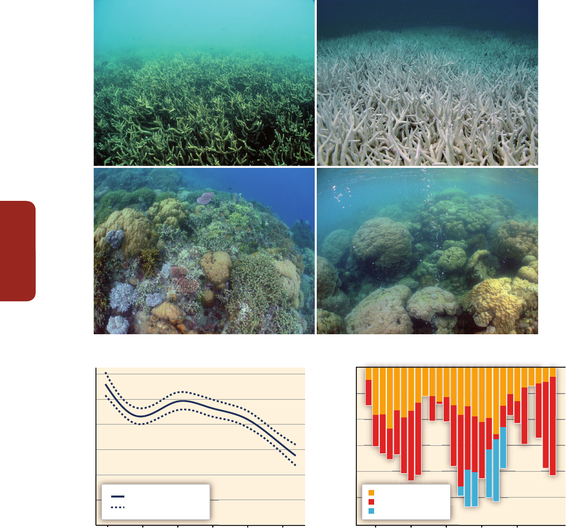
Figure CR-1 | (a, b) The same coral community before and after a bleaching event in February 2002 at 5 m depth, Halfway Island, Great Barrier Reef. Approximately 95% of the
coral community was severely bleached in 2002 (Elvidge et al., 2004). Corals experience increasing mortality as the intensity of a heating event increases. A few coral species
show the ability to shuffle symbiotic communities of dinoflagellates and appear to be more tolerant of warmer conditions (Berkelmans and van Oppen, 2006; Jones et al., 2008).
(c, d) Three CO
2
seeps in Milne Bay Province, Papua New Guinea show that prolonged exposure to high CO
2
is related to fundamental changes in the ecology of coral reefs
(Fabricius et al., 2011), including reduced coral diversity (–39%), severely reduced structural complexity (–67%), lower density of young corals (–66%), and fewer crustose
coralline algae (–85%). At high CO
2
sites (d; median pH
T
~7.8, where pH
T
is pH on the total scale), reefs are dominated by massive corals while corals with high morphological
complexity are underrepresented compared with control sites (c; median pH
T
~8.0). Reef development ceases at pH
T
values below 7.7. (e) Temporal trend in coral cover for the
whole Great Barrier Reef over the period 1985–2012 (N=number of reefs, De'ath et al., 2012). (f) Composite bars indicate the estimated mean coral mortality for each year, and
the sub-bars indicate the relative mortality due to crown-of-thorns starfish, cyclones, and bleaching for the whole Great Barrier Reef (De'ath et al., 2012). (Photo credit: R.
Berkelmans (a and b) and K. Fabricius (c and d).)

CR
Coral Reefs
Cross-Chapter Box
99
A growing number of studies have reported regional scale changes in coral calcification and mortality that are consistent with the scale and
impact of ocean warming and acidification when compared to local factors such as declining water quality and overfishing (Hoegh-Guldberg
et al., 2007). The abundance of reef building corals is in rapid decline in many Pacific and Southeast Asian regions (very high confidence, 1 to
2% per year for 1968–2004; Bruno and Selig, 2007). Similarly, the abundance of reef-building corals has decreased by more than 80% on many
Caribbean reefs (1977–2001; Gardner et al., 2003), with a dramatic phase shift from corals to seaweeds occurring on Jamaican reefs (Hughes,
1994). Tropical cyclones, coral predators, and thermal stress-related coral bleaching and mortality have led to a decline in coral cover on the
Great Barrier Reef by about 51% between 1985 and 2012 (Figure CR-1E and F). Although less well documented, benthic invertebrates other
than corals are also at risk (Przeslawski et al., 2008). Fish biodiversity is threatened by the permanent degradation of coral reefs, including in a
marine reserve (Jones et al., 2004).
Future impacts of climate-related drivers (ocean warming, acidification, sea level rise as well as more intense tropical cyclones and rainfall
events) will exacerbate the impacts of non-climate–related drivers (high confidence). Even under optimistic assumptions regarding corals being
able to rapidly adapt to thermal stress, one-third (9 to 60%, 68% uncertainty range) of the world’s coral reefs are projected to be subject to
long-term degradation (next few decades) under the Representative Concentration Pathway (RCP)3-PD scenario (Frieler et al., 2013). Under
the RCP4.5 scenario, this fraction increases to two-thirds (30 to 88%, 68% uncertainty range). If present-day corals have residual capacity to
acclimate and/or adapt, half of the coral reefs may avoid high-frequency bleaching through 2100 (limited evidence, limited agreement; Logan
et al., 2014). Evidence of corals adapting rapidly, however, to climate change is missing or equivocal (Hoegh-Guldberg, 2012).
Damage to coral reefs has implications for several key regional services:
• Resources: Coral reefs account for 10 to 12% of the fish caught in tropical countries, and 20 to 25% of the fish caught by developing
nations (Garcia and de Leiva Moreno, 2003). More than half (55%) of the 49 island countries considered by Newton et al. (2007) are
already exploiting their coral reef fisheries in an unsustainable way and the production of coral reef fish in the Pacific is projected to
decrease 20% by 2050 under the Special Report on Emission Scenarios (SRES) A2 emissions scenario (Bell et al., 2013).
• Coastal protection: Coral reefs contribute to protecting the shoreline from the destructive action of storm surges and cyclones (Sheppard
et al., 2005), sheltering the only habitable land for several island nations, habitats suitable for the establishment and maintenance of
mangroves and wetlands, as well as areas for recreational activities. This role is threatened by future sea level rise, the decrease in coral
cover, reduced rates of calcification, and higher rates of dissolution and bioerosion due to ocean warming and acidification (Sections
5.4.2.4, 6.4.1, 30.5).
• Tourism: More than 100 countries benefit from the recreational value provided by their coral reefs (Burke et al., 2011). For example, the
Great Barrier Reef Marine Park attracts about 1.9 million visits each year and generates A$5.4 billion to the Australian economy and
54,000 jobs (90% in the tourism sector; Biggs, 2011).
Coral reefs make a modest contribution to the global gross domestic product (GDP) but their economic importance can be high at the country
and regional scales (Pratchett et al., 2008). For example, tourism and fisheries represent 5% of the GDP of South Pacific islands (average for
2001–2011; Laurans et al., 2013). At the local scale, these two services provided in 2009–2011 at least 25% of the annual income of villages in
Vanuatu and Fiji (Pascal, 2011; Laurans et al., 2013).
Isolated reefs can recover from major disturbance, and the benefits of their isolation from chronic anthropogenic pressures can outweigh the
costs of limited connectivity (Gilmour et al., 2013). Marine protected areas (MPAs) and fisheries management have the potential to increase
ecosystem resilience and increase the recovery of coral reefs after climate change impacts such as mass coral bleaching (McLeod et al., 2009).
Although they are key conservation and management tools, they are unable to protect corals directly from thermal stress (Selig et al., 2012),
suggesting that they need to be complemented with additional and alternative strategies (Rau et al., 2012; Billé et al., 2013). While MPA
networks are a critical management tool, they should be established considering other forms of resource management (e.g., fishery catch limits
and gear restrictions) and integrated ocean and coastal management to control land-based threats such as pollution and sedimentation. There
is medium confidence that networks of highly protected areas nested within a broader management framework can contribute to preserving
coral reefs under increasing human pressure at local and global scales (Salm et al., 2006). Locally, controlling the input of nutrients and
sediment from land is an important complementary management strategy (Mcleod et al., 2009) because nutrient enrichment can increase the
susceptibility of corals to bleaching (Wiedenmann et al., 2013) and coastal pollutants enriched with fertilizers can increase acidification (Kelly
et al., 2011). In the long term, limiting the amount of ocean warming and acidification is central to ensuring the viability of coral reefs and
dependent communities (high confidence; Section 5.2.4.4, 30.5).
Bell, J.D., A. Ganachaud, P.C. Gehrke, S.P. Griffiths, A.J. Hobday, O. Hoegh-Guldberg, J.E. Johnson, R. Le Borgne, P. Lehodey, J.M. Lough, R.J. Matear, T.D. Pickering, M.S.
Pratchett, A. Sen Gupta, I. Senina and M. Waycott, 2013: Mixed responses of tropical Pacific fisheries and aquaculture to climate change. Nature Climate Change,
3(6), 591-599.
Berkelmans, R. and M.J.H. van Oppen, 2006: The role of zooxanthellae in the thermal tolerance of corals: a ‘nugget of hope’ for coral reefs in an era of climate change.
Proceedings of the Royal Society B: Biological Sciences, 273(1599), 2305-2312.
References

Cross-Chapter Box
Coral Reefs
100
CR
Biggs, D., 2011: Case study: the resilience of the nature-based tourism system on Australia’s Great Barrier Reef. Report prepared for the Australian Government
Department of Sustainability Environment Water Population and Communities on behalf of the State of the Environment 2011 Committee, Canberra, 32 pp.
Billé, R., R. Kelly, A. Biastoch, E. Harrould-Kolieb, D. Herr, F. Joos, K.J. Kroeker, D. Laffoley, A. Oschlies and J.-P. Gattuso, 2013: Taking action against ocean acidification: a
review of management and policy options. Environmental Management, 52, 761-779.
Bruno, J.F. and E.R. Selig, 2007: Regional decline of coral cover in the Indo-Pacific: timing, extent, and subregional comparisons. PLoS ONE, 2(8), e711. doi: 10.1371/
journal.pone.0000711.
Burke, L., K. Reytar, M. Spalding and A. Perry, 2011: Reefs at risk revisited. World Resources Institute, Washington D.C., 114 pp.
De’ath, G., K.E. Fabricius, H. Sweatman and M. Puotinen, 2012: The 27-year decline of coral cover on the Great Barrier Reef and its causes. Proceedings of the National
Academy of Sciences of the United States of America, 109(44), 17995-17999.
Elvidge, C.D., J.B. Dietz, R. Berkelmans, S. Andréfouët, W. Skirving, A.E. Strong and B.T. Tuttle, 2004: Satellite observation of Keppel Islands (Great Barrier Reef) 2002 coral
bleaching using IKONOS data. Coral Reefs, 23(1), 123-132.
Fabricius, K.E., C. Langdon, S. Uthicke, C. Humphrey, S. Noonan, G. De’ath, R. Okazaki, N. Muehllehner, M.S. Glas and J.M. Lough, 2011: Losers and winners in coral reefs
acclimatized to elevated carbon dioxide concentrations. Nature Climate Change, 1(3), 165-169.
Frieler, K., M. Meinshausen, A. Golly, M. Mengel, K. Lebek, S.D. Donner and O. Hoegh-Guldberg, 2013: Limiting global warming to 2°C is unlikely to save most coral reefs.
Nature Climate Change, 3(2), 165-170.
Garcia, S.M. and I. de Leiva Moreno, 2003: Global overview of marine fisheries. In: Responsible Fisheries in the Marine Ecosystem [Sinclair, M. and G. Valdimarsson (eds.)].
Wallingford: CABI, pp. 1-24.
Gardner, T.A., I.M. Côté, J.A. Gill, A. Grant and A.R. Watkinson, 2003: Long-term region-wide declines in Caribbean corals. Science, 301(5635), 958-960.
Gilmour, J.P., L.D. Smith, A.J. Heyward, A.H. Baird and M.S. Pratchett, 2013: Recovery of an isolated coral reef system following severe disturbance. Science, 340(6128),
69-71.
Glynn, P.W., 1984: Widespread coral mortality and the 1982-83 El Niño warming event. Environmental Conservation, 11(2), 133-146.
Hoegh-Guldberg, O., 2011: Coral reef ecosystems and anthropogenic climate change. Regional Environmental Change, 11, 215-227.
Hoegh-Guldberg, O., 2012: The adaptation of coral reefs to climate change: Is the Red Queen being outpaced? Scientia Marina, 76(2), 403-408.
Hoegh-Guldberg, O., P.J. Mumby, A.J. Hooten, R.S. Steneck, P. Greenfield, E. Gomez, C.D. Harvell, P.F. Sale, A.J. Edwards, K. Caldeira, N. Knowlton, C.M. Eakin, R. Iglesias-
Prieto, N. Muthiga, R.H. Bradbury, A. Dubi and M.E. Hatziolos, 2007: Coral reefs under rapid climate change and ocean acidification. Science, 318(5857), 1737-1742.
Hughes, T.P., 1994: Catastrophes, phase-shifts, and large-scale degradation of a Caribbean coral reef. Science, 265(5178), 1547-1551.
Jones, A.M., R. Berkelmans, M.J.H. van Oppen, J.C. Mieog and W. Sinclair, 2008: A community change in the algal endosymbionts of a scleractinian coral following a
natural bleaching event: field evidence of acclimatization. Proceedings of the Royal Society B: Biological Sciences, 275(1641), 1359-1365.
Jones, G.P., M.I. McCormick, M. Srinivasan and J.V. Eagle, 2004: Coral decline threatens fish biodiversity in marine reserves. Proceedings of the National Academy of
Sciences of the United States of America, 101(21), 8251-8253.
Kelly, R.P., M.M. Foley, W.S. Fisher, R.A. Feely, B.S. Halpern, G.G. Waldbusser and M.R. Caldwell, 2011: Mitigating local causes of ocean acidification with existing laws.
Science, 332(6033), 1036-1037.
Laurans, Y., N. Pascal, T. Binet, L. Brander, E. Clua, G. David, D. Rojat and A. Seidl, 2013: Economic valuation of ecosystem services from coral reefs in the South Pacific:
taking stock of recent experience. Journal of Environmental Management, 116, 135-144.
Logan, C.A., J.P. Dunne, C.M. Eakin and S.D. Donner, 2014: Incorporating adaptive responses into future projections of coral bleaching. Global Change Biology, 20(1),
125-139.
Lough, J.M., 2000: 1997–98: Unprecedented thermal stress to coral reefs? Geophysical Research Letters, 27(23), 3901-3904.
McLeod, E., R. Salm, A. Green and J. Almany, 2009: Designing marine protected area networks to address the impacts of climate change. Frontiers in Ecology and the
Environment, 7(7), 362-370.
Newton, K., I.M. Côté, G.M. Pilling, S. Jennings and N.K. Dulvy, 2007: Current and future sustainability of island coral reef fisheries. Current Biology, 17(7), 655-658.
Pascal, N., 2011: Cost-benefit analysis of community-based marine protected areas: 5 case studies in Vanuatu, South Pacific. CRISP Research Reports. CRIOBE (EPHE/
CNRS). Insular Research Center and Environment Observatory, Mooréa, French Polynesia, 107 pp.
Pratchett, M.S., P.L. Munday, S.K. Wilson, N.A.J. Graham, J.E. Cinner, D.R. Bellwood, G.P. Jones, N.V.C. Polunin and T.R. McClanahan, 2008: Effects of climate-induced coral
bleaching on coral-reef fishes - Ecological and economic consequences. Oceanography and Marine Biology: An Annual Review, 46, 251-296.
Przeslawski, R., S. Ahyong, M. Byrne, G. Wörheide and P. Hutchings, 2008: Beyond corals and fish: the effects of climate change on noncoral benthic invertebrates of
tropical reefs. Global Change Biology, 14(12), 2773-2795.
Rau, G.H., E.L. McLeod and O. Hoegh-Guldberg, 2012: The need for new ocean conservation strategies in a high-carbon dioxide world. Nature Climate Change, 2(10),
720-724.
Salm, R.V., T. Done and E. McLeod, 2006: Marine Protected Area planning in a changing climate. In: Coastal and Estuarine Studies 61. Coral Reefs and Climate Change:
Science and Management. [Phinney, J.T., O. Hoegh-Guldberg, J. Kleypas, W. Skirving and A. Strong (eds.)]. American Geophysical Union, pp. 207-221.
Selig, E.R., K.S. Casey and J.F. Bruno, 2012: Temperature-driven coral decline: the role of marine protected areas. Global Change Biology, 18(5), 1561-1570.
Sheppard, C., D.J. Dixon, M. Gourlay, A. Sheppard and R. Payet, 2005: Coral mortality increases wave energy reaching shores protected by reef flats: Examples from the
Seychelles. Estuarine, Coastal and Shelf Science, 64(2-3), 223-234.
Wiedenmann, J., C. D’Angelo, E.G. Smith, A.N. Hunt, F.-E. Legiret, A.D. Postle and E.P. Achterberg, 2013: Nutrient enrichment can increase the susceptibility of reef corals
to bleaching. Nature Climate Change, 3(2), 160-164.
Wild, C., O. Hoegh-Guldberg, M.S. Naumann, M.F. Colombo-Pallotta, M. Ateweberhan, W.K. Fitt, R. Iglesias-Prieto, C. Palmer, J.C. Bythell, J.-C. Ortiz, Y. Loya and R. van
Woesik, 2011: Climate change impedes scleractinian corals as primary reef ecosystem engineers. Marine and Freshwater Research, 62(2), 205-215.
Gattuso, J.-P., O. Hoegh-Guldberg, and H.-O. Pörtner, 2014: Cross-chapter box on coral reefs. In: Climate Change 2014: Impacts, Adaptation, and Vulnerability.
Part A: Global and Sectoral Aspects. Contribution of Working Group II to the Fifth Assessment Report of the Intergovernmental Panel on Climate Change
[Field, C.B., V.R. Barros, D.J. Dokken, K.J. Mach, M.D. Mastrandrea, T.E. Bilir, M. Chatterjee, K.L. Ebi, Y.O. Estrada, R.C. Genova, B. Girma, E.S. Kissel, A.N. Levy,
S. MacCracken, P.R. Mastrandrea, and L.L. White (eds.)]. Cambridge University Press, Cambridge, United Kingdom and New York, NY, USA, pp. 97-100.
This cross-chapter box should be cited as:

Ecosystem-Based
Approaches to Adaptation—
Emerging Opportunities
Rebecca Shaw (USA), Jonathan Overpeck (USA), Guy Midgley (South Africa)
EA
101
Ecosystem-based adaptation (EBA), defined as the use of biodiversity and ecosystem services as
part of an overall adaptation strategy to help people to adapt to the adverse effects of climate
change (CBD, 2009), integrates the use of biodiversity and ecosystem services into climate
change adaptation strategies (e.g., CBD, 2009; Munroe et al., 2011; see IPCC AR5 WGII Chapters
3, 4, 5, 8, 9, 13, 14, 15, 16, 19, 22, 25, and 27). EBA is implemented through the sustainable
management of natural resources and conservation and restoration of ecosystems, to provide
and sustain services that facilitate adaptation both to climate variability and change (Colls et al.,
2009). It also sets out to take into account the multiple social, economic, and cultural co-benefits
for local communities (CBD COP 10 Decision X/33).
EBA can be combined with, or even serve as a substitute for, the use of engineered infrastructure
or other technological approaches. Engineered defenses such as dams, sea walls, and levees
adversely affect biodiversity, potentially resulting in maladaptation due to damage to ecosystem
regulating services (Campbell et al., 2009; Munroe et al., 2011). There is some evidence that the
restoration and use of ecosystem services may reduce or delay the need for these engineering
solutions (CBD, 2009). EBA offers lower risk of maladaptation than engineering solutions in
that their application is more flexible and responsive to unanticipated environmental changes.
Well-integrated EBA can be more cost effective and sustainable than non-integrated physical
engineering approaches (Jones et al., 2012), and may contribute to achieving sustainable
development goals (e.g., poverty reduction, sustainable environmental management, and even
mitigation objectives), especially when they are integrated with sound ecosystem management
approaches (CBD, 2009). In addition, EBA yields economic, social, and environmental co-benefits
in the form of ecosystem goods and services (World Bank, 2009).
EBA is applicable in both developed and developing countries. In developing countries where
economies depend more directly on the provision of ecosystem services (Vignola et al., 2009),
EBA may be a highly useful approach to reduce risks to climate change impacts and ensure that
development proceeds on a pathways that are resilient to climate change (Munang et al., 2013).
EBA projects may be developed by enhancing existing initiatives, such as community-based
adaptation and natural resource management approaches (e.g., Khan et al., 2012, Midgley et al.,
2012; Roberts et al., 2012).
Examples of ecosystem based approaches to adaptation include:
• Sustainable water management, where river basins, aquifers, flood plains, and their
associated vegetation are managed or restored to provide resilient water storage and

Cross-Chapter Box
Ecosystem-Based Approaches to Adaptation–Emerging Opportunities
102
EA
enhanced baseflows, flood regulation and protection services, reduction of erosion/siltation rates, and more ecosystem goods (e.g.,
Opperman et al., 2009; Midgley et al., 2012)
• Disaster risk reduction through the restoration of coastal habitats (e.g., mangroves, wetlands, and deltas) to provide effective measure
against storm-surges, saline intrusion, and coastal erosion (Jonkman et al., 2013)
• Sustainable management of grasslands and rangelands to enhance pastoral livelihoods and increase resilience to drought and flooding
• Establishment of diverse and resilient agricultural systems, and adapting crop and livestock variety mixes to secure food provision.
Traditional knowledge may contribute in this area through, for example, identifying indigenous crop and livestock genetic diversity, and
water conservation techniques.
• Management of fire-prone ecosystems to achieve safer fire regimes while ensuring the maintenance of natural processes
Application of EBA, like other approaches, is not without risk, and risk/benefit assessments will allow better assessment of opportunities
offered by the approach (CBD, 2009). The examples of EBA are too few and too recent to assess either the risks or the benefits comprehensively
at this stage. EBA is still a developing concept but should be considered alongside adaptation options based more on engineering works or
social change, and existing and new cases used to build understanding of when and where its use is appropriate.
Climate mitigation Climate change impacts
Ecosystem protection
and restoration
Sustainable
economies with
reduced risk of
climate impacts
Increase in human well-being
Sustained ecosystem
services delivery
Biodiversity retention,
ecosystem resilience, and
reduced vulnerability
Degradation of
ecological processes
and loss of biodiversity
Loss of
ecosystem
services
Loss of human
well-being
Increased pressure
on ecosystems/
natural capital
With ecosystem-based
adaptation
Without ecosystem-based
adaptation
Figure EA-1 |
Adapted from Munang et al. (2013). Ecosystem-based adaptation (EBA) uses the capacity of nature to buffer human systems from the adverse impacts of climate
change. Without EBA, climate change may cause degradation of ecological processes (central white panel) leading to losses in human well-being. Implementing EBA (outer blue
panel) may reduce or offset these adverse impacts resulting in a virtuous cycle that reduces climate-related risks to human communities, and may provide mitigation benefits.
Campbell, A., V. Kapos, J. Scharlemann, P. Bubb, A. Chenery, L. Coad, B. Dickson, N. Doswald, M. Khan, F. Kershaw, and M. Rashid, 2009: Review of the Literature on
the Links between Biodiversity and Climate Change: Impacts, Adaptation and Mitigation. CBD Technical Series No. 42, Secretariat of the Convention on Biological
Diversity (CBD), Montreal, QC, Canada, 124 pp.
CBD, 2009: Connecting Biodiversity and Climate Change Mitigation and Adaptation: Report of the Second Ad Hoc Technical Expert Group on Biodiversity and Climate
Change. CBD Technical Series No. 41, Secretariat of the Convention on Biological Diversity (CBD), Montreal, QC, Canada, 126 pp.
Colls, A., N. Ash, and N. Ikkala, 2009: Ecosystem-Based Adaptation: A Natural Response to Climate Change. International Union for Conservation of Nature and Natural
Resources (IUCN), Gland, Switzerland, 16 pp.
Jones, H.P., D.G. Hole, and E.S. Zavaleta, 2012: Harnessing nature to help people adapt to climate change. Nature Climate Change, 2(7), 504-509.
Jonkman, S.N., M.M. Hillen, R.J. Nicholls, W. Kanning, and M. van Ledden, 2013: Costs of adapting coastal defences to sea-level rise – new estimates and their
implications. Journal of Coastal Research, 29(5), 1212-1226.
Khan, A.S., A. Ramachandran, N. Usha, S. Punitha, and V. Selvam, 2012: Predicted impact of the sea-level rise at Vellar-Coleroon estuarine region of Tamil Nadu coast in
India: mainstreaming adaptation as a coastal zone management option. Ocean & Coastal Management, 69, 327-339.
Midgley, G.F., S. Marais, M. Barnett, and K. Wågsæther, 2012: Biodiversity, Climate Change and Sustainable Development – Harnessing Synergies and Celebrating
Successes. Final Technical Report, The Adaptation Network Secretariat, hosted by Indigo Development & Change and The Environmental Monitoring Group,
Nieuwoudtville, South Africa. 70 pp.
Munang, R, I. Thiaw, K. ALverson, M. Mumba, J. Liu, and M. Rivington, 2013: Climate change and ecosystem-based adaptation: a new pragmatic approach to buffering
climate change impacts. Current Opinion in Environmental Sustainability, 5(1), 67-71.
Munroe, R., N. Doswald, D. Roe, H. Reid, A. Giuliani, I. Castelli, and I. Moller, 2011: Does EbA Work? A Review of the Evidence on the Effectiveness of Ecosystem-Based
Approaches to Adaptation. Research collaboration between BirdLife International, United Nations Environment Programme-World Conservation Monitoring Centre
(UNEP-WCMC), and the University of Cambridge, Cambridge, UK, and the International Institute for Environment and Development (IIED), London, UK, 4 pp.
References

EA
Ecosystem-Based Approaches to Adaptation–Emerging Opportunities
Cross-Chapter Box
103
Opperman, J.J., G.E. Galloway, J. Fargione, J.F. Mount, B.D. Richter, and S. Secchi, 2009: Sustainable floodplains through large-scale reconnection to rivers. Science,
326(5959), 1487-1488.
Roberts, D., R. Boon, N. Diederichs, E. Douwes, N. Govender, A. McInnes, C. McLean, S. O’Donoghue, and M. Spires, 2012: Exploring ecosystem-based adaptation in
Durban, South Africa: “learning-by-doing” at the local government coal face. Environment and Urbanization, 24(1), 167-195.
Vignola, R., B. Locatelli, C. Martinez, and P. Imbach, 2009: Ecosystem-based adaptation to climate change: what role for policymakers, society and scientists? Mitigation
and Adaptation Strategies for Global Change, 14(8), 691-696.
Shaw, M.R., J.T. Overpeck, and G.F. Midgley, 2014: Cross-chapter box on ecosystem based approaches to adaptation—emerging opportunities. In: Climate
Change 2014: Impacts, Adaptation, and Vulnerability. Part A: Global and Sectoral Aspects. Contribution of Working Group II to the Fifth Assessment Report
of the Intergovernmental Panel on Climate Change [Field, C.B., V.R. Barros, D.J. Dokken, K.J. Mach, M.D. Mastrandrea, T.E. Bilir, M. Chatterjee, K.L. Ebi, Y.O.
Estrada, R.C. Genova, B. Girma, E.S. Kissel, A.N. Levy, S. MacCracken, P.R. Mastrandrea, and L.L. White (eds.)]. Cambridge University Press, Cambridge,
United Kingdom and New York, NY, USA, pp. 101-103.
This cross-chapter box should be cited as:

Gender and Climate Change
Katharine Vincent (South Africa), Petra Tschakert (U.S.A.), Jon Barnett (Australia), Marta G.
Rivera-Ferre (Spain), Alistair Woodward (New Zealand)
GC
105
Gender, along with sociodemographic factors of age, wealth, and class, is critical to the ways
in which climate change is experienced. There are significant gender dimensions to impacts,
adaptation, and vulnerability. This issue was raised in WGII AR4 and SREX reports (Adger et
al., 2007; IPCC, 2012), but for the AR5 there are significant new findings, based on multiple
lines of evidence on how climate change is differentiated by gender, and how climate change
contributes to perpetuating existing gender inequalities. This new research has been undertaken
in every region of the world (e.g. Brouwer et al., 2007; Buechler, 2009; Nelson and Stathers,
2009; Nightingale, 2009; Dankelman, 2010; MacGregor, 2010; Alston, 2011; Arora-Jonsson, 2011;
Omolo, 2011; Resureccion, 2011).
Gender dimensions of vulnerability derive from differential access to the social and environmental
resources required for adaptation. In many rural economies and resource-based livelihood
systems, it is well established that women have poorer access than men to financial resources,
land, education, health, and other basic rights. Further drivers of gender inequality stem
from social exclusion from decision-making processes and labor markets, making women in
particular less able to cope with and adapt to climate change impacts (Paavola, 2008; Djoudi
and Brockhaus, 2011; Rijkers and Costa, 2012). These gender inequalities manifest themselves in
gendered livelihood impacts and feminisation of responsibilities: whereas both men and women
experience increases in productive roles, only women experience increased reproductive roles
(Resureccion, 2011; Section 9.3.5.1.5, Box 13-1). A study in Australia, for example, showed how
more regular occurrence of drought has put women under increasing pressure to earn off-farm
income and contribute to more on-farm labor (Alston, 2011). Studies in Tanzania and Malawi
demonstrate how women experience food and nutrition insecurity because food is preferentially
distributed among other family members (Nelson and Stathers, 2009; Kakota et al., 2011).
AR4 assessed a body of literature that focused on women’s relatively higher vulnerability to
weather-related disasters in terms of number of deaths (Adger et al., 2007). Additional literature
published since that time adds nuances by showing how socially constructed gender differences
affect exposure to extreme events, leading to differential patterns of mortality for both men and
women (high confidence; Section 11.3.3, Table 12-3). Statistical evidence of patterns of male and
female mortality from recorded extreme events in 141 countries between 1981 and 2002 found
that disasters kill women at an earlier age than men (Neumayer and Plümper, 2007; see also
Box 13-1). Reasons for gendered differences in mortality include various socially and culturally
determined gender roles. Studies in Bangladesh, for example, show that women do not learn to
swim and so are vulnerable when exposed to flooding (Röhr, 2006) and that, in Nicaragua, the
construction of gender roles means that middle-class women are expected to stay in the house,

Cross-Chapter Box
Gender and Climate Change
106
GC
even during floods and in risk-prone areas (Bradshaw, 2010). Although the differential vulnerability of women to extreme events has long
been understood, there is now increasing evidence to show how gender roles for men can affect their vulnerability. In particular, men are often
expected to be brave and heroic, and engage in risky life-saving behaviors that increase their likelihood of mortality (Box 13-1). In Hai Lang
district, Vietnam, for example, more men died than women as a result of their involvement in search and rescue and protection of fields during
flooding (Campbell et al., 2009). Women and girls are more likely to become victims of domestic violence after a disaster, particularly when
they are living in emergency accommodation, which has been documented in the USA and Australia (Jenkins and Phillips, 2008; Anastario et
al., 2009; Alston, 2011; Whittenbury, 2013; see also Box 13-1).
Heat stress exhibits gendered differences, reflecting both physiological and social factors (Section 11.3.3). The majority of studies in European
countries show women to be more at risk, but their usually higher physiological vulnerability can be offset in some circumstances by relatively
lower social vulnerability (if they are well connected in supportive social networks, for example). During the Paris heat wave, unmarried men
were at greater risk than unmarried women, and in Chicago elderly men were at greatest risk, thought to reflect their lack of connectedness
in social support networks which led to higher social vulnerability (Kovats and Hajat, 2008). A multi-city study showed geographical variations
in the relationship between sex and mortality due to heat stress: in Mexico City, women had a higher risk of mortality than men, although the
reverse was true in Santiago and São Paulo (Bell et al., 2008).
Recognizing gender differences in vulnerability and adaptation can enable gender-sensitive responses that reduce the vulnerability of women
and men (Alston, 2013). Evaluations of adaptation investments demonstrate that those approaches that are not sensitive to gender dimensions
and other drivers of social inequalities risk reinforcing existing vulnerabilities (Vincent et al., 2010; Arora-Jonsson, 2011; Figueiredo and Perkins,
2012). Government-supported interventions to improve production through cash-cropping and non-farm enterprises in rural economies, for
example, typically advantage men over women because cash generation is seen as a male activity in rural areas (Gladwin et al., 2001; see
also Section 13.3.1). In contrast, rainwater and conservation-based adaptation initiatives may require additional labor, which women cannot
necessarily afford to provide (Baiphethi et al., 2008). Encouraging gender-equitable access to education and strengthening of social capital
are among the best means of improving adaptation of rural women farmers (Goulden et al., 2009; Vincent et al., 2010; Below et al., 2012) and
could be used to complement existing initiatives mentioned above that benefit men. Rights-based approaches to development can inform
adaptation efforts as they focus on addressing the ways in which institutional practices shape access to resources and control over decision-
making processes, including through the social construction of gender and its intersection with other factors that shape inequalities and
vulnerabilities (Tschakert and Machado, 2012; Bee et al., 2013; Tschakert, 2013; see also Section 22.4.3 and Table 22-5).
Adger, W.N., S. Agrawala, M.M.Q. Mirza, C. Conde, K. O’Brien, J. Pulhin, R. Pulwarty, B. Smit, and K. Takahashi, 2007: Chapter 17: Assessment of adaptation practices,
options, constraints and capacity. In: Climate Change 2007: Impacts, Adaptation and Vulnerability. Contribution of Working Group II to the Fourth Assessment Report
of the Intergovernmental Panel on Climate Change [Parry, M.L., O.F. Canziani, J.P. Palutikof, P.J. van der Linden, and C.E. Hanson (ed.)]. IPCC, Geneva, Switzerland, pp.
719-743.
Alston, M., 2011: Gender and climate change in Australia. Journal of Sociology, 47(1), 53-70.
Alston, M., 2013: Women and adaptation. Wiley Interdisciplinary Reviews: Climate Change, (4)5, 351-358.
Anastario, M., N. Shebab, and L. Lawry, 2009: Increased gender-based violence among women internally displaced in Mississippi 2 years post-Hurricane Katrina. Disaster
Medicine and Public Health Preparedness, 3(1), 18-26.
Arora-Jonsson, S., 2011: Virtue and vulnerability: discourses on women, gender and climate change. Global Environmental Change, 21, 744-751.
Baiphethi, M.N., M. Viljoen, and G. Kundhlande, 2008: Rural women and rainwater harvesting and conservation practices: anecdotal evidence from the Free State and
Eastern Cape. Agenda, 22(78), 163-171.
Bee, B., M. Biermann, and P. Tschakert, 2013: Gender, development, and rights-based approaches: lessons for climate change adaptation and adaptive social protection.
In: Research, Action and Policy: Addressing the Gendered Impacts of Climate Change [Alston, M. and K. Whittenbury (eds.)]. Springer, Dordrecht, Netherlands, pp.
95-108.
Bell, M.L., M.S. O’Neill, N. Ranjit, V.H. Borja-Aburto, L.A. Cifuentes, and N.C. Gouveia, 2008: Vulnerability to heat-related mortality in Latin America: a case-crossover study
in Sao Paulo, Brazil, Santiago, Chile and Mexico City, Mexico. International Journal of Epidemiology, 37(4), 796-804.
Below, T.B., K.D. Mutabazi, D. Kirschke, C. Franke, S. Sieber, R. Siebert, and K. Tscherning, 2012: Can farmers’ adaptation to climate change be explained by socio-economic
household-level variables? Global Environmental Change, 22(1), 223-235.
Bradshaw, S., 2010: Women, poverty, and disasters: exploring the links through Hurricane Mitch in Nicaragua. In: The International Handbook of Gender and Poverty:
Concepts, Research, Policy [Chant, S. (ed.)]. Edward Elgar Publishing, Cheltenham, UK, pp. 627-632.
Brouwer, R., S. Akter, L. Brander, and E. Haque, 2007: Socioeconomic vulnerability and adaptation to environmental risk: a case study of climate change and flooding in
Bangladesh. Risk Analysis, 27(2), 313-326.
Campbell, B., S. Mitchell, and M. Blackett, 2009: Responding to Climate Change in Vietnam. Opportunities for Improving Gender Equality. A Policy Discussion Paper,
Oxfam in Viet Nam and United Nations Development Programme-Viet Nam (UNDP-Viet Nam), Ha noi, Viet Nam, 62 pp.
Dankelman, I., 2010: Introduction: exploring gender, environment, and climate change. In: Gender and Climate Change: An Introduction [Dankelman, I. (ed.)]. Earthscan,
London, UK and Washington, DC, USA, pp. 1-18.
Djoudi, H. and M. Brockhaus, 2011: Is adaptation to climate change gender neutral? Lessons from communities dependent on livestock and forests in northern Mali.
International Forestry Review, 13(2), 123-135.
Figueiredo, P. and P.E. Perkins, 2012: Women and water management in times of climate change: participatory and inclusive processes. Journal of Cleaner Production,
60(1), 188-194.
References

GC
Gender and Climate Change
Cross-Chapter Box
107
Gladwin, C.H., A.M. Thomson, J.S. Peterson, and A.S. Anderson, 2001: Addressing food security in Africa via multiple livelihood strategies of women farmers. Food Policy,
26(2), 177-207.
Goulden, M., L.O. Naess, K. Vincent, and W.N. Adger, 2009: Diversification, networks and traditional resource management as adaptations to climate extremes in rural
Africa: opportunities and barriers. In: Adapting to Climate Change: Thresholds, Values and Governance [Adger, W.N., I. Lorenzoni, and K. O’Brien (eds.)]. Cambridge
University Press, Cambridge, UK, pp. 448-464.
IPCC, 2012: Managing the Risks of Extreme Events and Disasters to Advance Climate Change Adaptation. A Special Report of Working Groups I and II of the
Intergovernmental Panel on Climate Change [Field, C.B., V. Barros, T.F. Stocker, D. Qin, D.J. Dokken, K.L. Ebi, M.D. Mastrandrea, K.J. Mach, G.-K. Plattner, S.K. Allen, M.
Tignor, and P.M. Midgley (eds.)], Cambridge University Press, Cambridge, UK and New York, NY, USA, 582 pp.
Jenkins, P. and B. Phillips, 2008: Battered women, catastrophe, and the context of safety after Hurricane Katrina. NWSA Journal, 20(3), 49-68.
Kakota, T., D. Nyariki, D. Mkwambisi, and W. Kogi-Makau, 2011: Gender vulnerability to climate variability and household food insecurity. Climate and Development, 3(4),
298-309.
Kovats, R. and S. Hajat, 2008: Heat stress and public health: a critical review. Public Health, 29, 41-55.
MacGregor, S., 2010: ‘Gender and climate change’: from impacts to discourses. Journal of the Indian Ocean Region, 6(2), 223-238.
Nelson, V. and T. Stathers, 2009: Resilience, power, culture, and climate: a case study from semi-arid Tanzania, and new research directions. Gender & Development, 17(1),
81-94.
Neumayer, E. and T. Plümper, 2007: The gendered nature of natural disasters: the impact of catastrophic events on the gender gap in life expectancy, 1981-2002. Annals
of the Association of American Geographers, 97(3), 551-566.
Nightingale, A., 2009: Warming up the climate change debate: a challenge to policy based on adaptation. Journal of Forest and Livelihood, 8(1), 84-89.
Omolo, N., 2011: Gender and climate change-induced conflict in pastoral communities: case study of Turkana in northwestern Kenya. African Journal on Conflict
Resolution, 10(2), 81-102.
Paavola, J., 2008: Livelihoods, vulnerability and adaptation to climate change in Morogoro, Tanzania. Environmental Science & Policy, 11(7), 642-654.
Resurreccion, B.P., 2011: The Gender and Climate Debate: More of the Same or New Pathways of Thinking and Doing? Asia Security Initiative Policy Series, Working Paper
No. 10, RSIS Centre for Non-Traditional Security (NTS) Studies, Singapore, 19 pp.
Rijkers, B. and R. Costa, 2012: Gender and Rural Non-Farm Entrepreneurship. Policy Research Working Paper 6066, Macroeconomics and Growth Team, Development
Research Group, The World Bank, Washington, DC, USA, 68 pp.
Röhr, U., 2006: Gender and climate change. Tiempo, 59, 3-7.
Tschakert, P., 2013: From impacts to embodied experiences: tracing political ecology in climate change research. Geografisk Tidsskrift/Danish Journal of Geography,
112(2), 144-158.
Tschakert, P. and M. Machado, 2012: Gender justice and rights in climate change adaptation: opportunities and pitfalls. Ethics and Social Welfare, 6(3), 275-289, doi:
10.1080/17496535.2012.704929.
Vincent, K., T. Cull, and E. Archer, 2010: Gendered vulnerability to climate change in Limpopo province, South Africa. In: Gender and Climate Change: An Introduction
[Dankelman, I. (ed.)]. Earthscan, London, UK and Washington, DC, USA, pp. 160-167.
Whittenbury, K., 2013: Climate change, women’s health, wellbeing and experiences of gender-based violence in Australia. In: Research, Action and Policy: Addressing the
Gendered Impacts of Climate Change [Alston, M. and K. Whittenbury (eds.)]. Springer Science, Dordrecht, Netherlands, pp. 207-222.
K.E. Vincent, P. Tschakert, Barnett, J., M.G. Rivera-Ferre, and A. Woodward, 2014: Cross-chapter box on gender and climate change. In: Climate Change 2014:
Impacts, Adaptation, and Vulnerability. Part A: Global and Sectoral Aspects. Contribution of Working Group II to the Fifth Assessment Report of the
Intergovernmental Panel on Climate Change [Field, C.B., V.R. Barros, D.J. Dokken, K.J. Mach, M.D. Mastrandrea, T.E. Bilir, M. Chatterjee, K.L. Ebi, Y.O. Estrada,
R.C. Genova, B. Girma, E.S. Kissel, A.N. Levy, S. MacCracken, P.R. Mastrandrea, and L.L. White (eds.)]. Cambridge University Press, Cambridge, United
Kingdom and New York, NY, USA, pp. 105-107.
This cross-chapter box should be cited as:

Heat Stress and Heat Waves
Lennart Olsson (Sweden), Dave Chadee (Trinidad and Tobago), Ove Hoegh-Guldberg (Australia),
Michael Oppenheimer (USA), John Porter (Denmark), Hans-O. Pörtner (Germany), David
Satterthwaite (UK),Kirk R. Smith (USA), Maria Isabel Travasso (Argentina), Petra Tschakert (USA)
HS
109
According to WGI, it is very likely that the number and intensity of hot days have increased
markedly in the last three decades and virtually certain that this increase will continue into
the late 21st century. In addition, it is likely (medium confidence) that the occurrence of heat
waves (multiple days of hot weather in a row) has more than doubled in some locations, but
very likely that there will be more frequent heat waves over most land areas after mid-century.
Under a medium warming scenario, Coumou et al. (2013) predicted that the number of monthly
heat records will be more than 12 times more common by the 2040s compared to a non-
warming world. In a longer time perspective, if the global mean temperature increases to +7°C
or more, the habitability of parts of the tropics and mid-latitudes will be at risk (Sherwood and
Huber, 2010). Heat waves affect natural and human systems directly, often with severe losses
of lives and assets as a result, and may act as triggers of tipping points (Hughes et al., 2013).
Consequently, heat stress plays an important role in several key risks noted in Chapter 19 and
CC-KR.
Economy and Society (Chapters 10, 11, 12, 13)
Environmental heat stress has already reduced the global labor capacity to 90% in peak months
with a further predicted reduction to 80% in peak months by 2050. Under a high warming
scenario (RCP8.5), labor capacity is expected to be less than 40% of present-day conditions in
peak months by 2200 (Dunne et al., 2013). Adaptation costs for securing cooling capacities and
emergency shelters during heat waves will be substantial.
Heat waves are associated with social predicaments such as increasing violence (Anderson,
2012) as well as overall health and psychological distress and low life satisfaction (Tawatsupa
et al., 2012). Impacts are highly differential with disproportional burdens on poor people, elderly
people, and those who are marginalized (Wilhelmi et al., 2012). Urban areas are expected to
suffer more due to the combined effect of climate and the urban heat island effect (Fischer et al.,
2012; see also Section 8.2.3.1). In low- and medium-income countries, adaptation to heat stress
is severely restricted for most people in poverty and particularly those who are dependent on
working outdoors in agriculture, fisheries, and construction. In small-scale agriculture, women and
children are particularly at risk due to the gendered division of labor (Croppenstedt et al., 2013).
The expected increase in wildfires as a result of heat waves (Pechony and Shindell, 2010) is a
concern for human security, health, and ecosystems. Air pollution from wildfires already causes an
estimated 339,000 premature deaths per year worldwide (Johnston et al., 2012).

Cross-Chapter Box
Heat Stress
110
HS
Human Health (Chapter 11)
Morbidity and mortality due to heat stress is now common all over the world (Barriopedro et al., 2011; Nitschke et al., 2011; Rahmstorf
and Coumou, 2011; Diboulo et al., 2012; Hansen et al., 2012). Elderly people and people with circulatory and respiratory diseases are also
vulnerable even in developed countries; they can become victims even inside their own houses (Honda et al., 2011). People in physical work are
at particular risk as such work produces substantial heat within the body, which cannot be released if the outside temperature and humidity
is above certain limits (Kjellstrom et al., 2009). The risk of non-melanoma skin cancer from exposure to UV radiation during summer months
increases with temperature (van der Leun, et al., 2008). High temperatures are also associated with an increase in air-borne allergens acting as
triggers for respiratory illnesses such as asthma, allergic rhinitis, conjunctivitis, and dermatitis (Beggs, 2010).
Ecosystems (Chapters 4, 5, 6, 30)
Tree mortality is increasing globally (Williams et al., 2013) and can be linked to climate impacts, especially heat and drought (Reichstein et al.,
2013), even though attribution to climate change is difficult owing to lack of time series and confounding factors. In the Mediterranean region,
higher fire risk, longer fire season, and more frequent large, severe fires are expected as a result of increasing heat waves in combination with
drought (Duguy et al., 2013; see also Box 4.2).
Marine ecosystem shifts attributed to climate change are often caused by temperature extremes rather than changes in the average (Pörtner
and Knust, 2007). During heat exposure near biogeographical limits, even small (<0.5°C) shifts in temperature extremes can have large effects,
often exacerbated by concomitant exposures to hypoxia and/or elevated CO
2
levels and associated acidification (medium confidence; Hoegh-
Guldberg et al., 2007; see also Figure 6-5; Sections 6.3.1, 6.3.5, 30.4, 30.5; CC-MB).
Most coral reefs have experienced heat stress sufficient to cause frequent mass coral bleaching events in the last 30 years, sometimes
followed by mass mortality (Baker et al., 2008). The interaction of acidification and warming exacerbates coral bleaching and mortality (very
high confidence).Temperate seagrass and kelp ecosystems will decline with the increased frequency of heat waves and through the impact of
invasive subtropical species (high confidence; Sections 5, 6, 30.4, 30.5, CC-CR, CC-MB).
Agriculture (Chapter 7)
Excessive heat interacts with key physiological processes in crops. Negative yield impacts for all crops past +3°C of local warming without
adaptation, even with benefits of higher CO
2
and rainfall, are expected even in cool environments (Teixeira et al., 2013). For tropical systems
where moisture availability or extreme heat limits the length of the growing season, there is a high potential for a decline in the length of the
growing season and suitability for crops (medium evidence, medium agreement; Jones and Thornton, 2009). For example, half of the wheat-
growing area of the Indo-Gangetic Plains could become significantly heat-stressed by the 2050s.
There is high confidence that high temperatures reduce animal feeding and growth rates (Thornton et al., 2009). Heat stress reduces
reproductive rates of livestock (Hansen, 2009), weakens their overall performance (Henry et al., 2012), and may cause mass mortality of
animals in feedlots during heat waves (Polley et al., 2013). In the USA, current economic losses due to heat stress of livestock are estimated at
several billion US$ annually (St-Pierre et al., 2003).
Anderson, C.A., 2012: Climate change and violence. In: The Encyclopedia of Peace Psychology [Christie, D.J. (ed.)]. John Wiley & Sons/Blackwell, Chichester, UK, pp. 128-
132.
Baker, A.C., P.W. Glynn, and B. Riegl, 2008: Climate change and coral reef bleaching: an ecological assessment of long-term impacts, recovery trends and future outlook.
Estuarine, Coastal and Shelf Science, 80(4), 435-471.
Barriopedro, D., E.M. Fischer, J. Luterbacher, R.M. Trigo, and R. García-Herrera, 2011: The hot summer of 2010: redrawing the temperature record map of Europe. Science,
332(6026), 220-224.
Beggs, P.J., 2010: Adaptation to impacts of climate change on aeroallergens and allergic respiratory diseases. International Journal of Environmental Research and Public
Health, 7(8), 3006-3021.
Coumou, D., A. Robinson, and S. Rahmstorf, 2013: Global increase in record-breaking monthly-mean temperatures. Climatic Change, 118(3-4), 771-782.
Croppenstedt, A., M. Goldstein, and N. Rosas, 2013: Gender and agriculture: inefficiencies, segregation, and low productivity traps. The World Bank Research Observer,
28(1), 79-109.
Diboulo, E., A. Sie, J. Rocklöv, L. Niamba, M. Ye, C. Bagagnan, and R. Sauerborn, 2012: Weather and mortality: a 10 year retrospective analysis of the Nouna Health and
Demographic Surveillance System, Burkina Faso. Global Health Action, 5, 19078, doi:10.3402/gha.v5i0.19078.
Duguy, B., S. Paula, J.G. Pausas, J.A. Alloza, T. Gimeno, and R.V. Vallejo, 2013: Effects of climate and extreme events on wildfire regime and their ecological impacts. In:
Regional Assessment of Climate Change in the Mediterranean, Volume 3: Case Studies [Navarra, A. and L. Tubiana (eds.)]. Advances in Global Change Research
Series: Vol. 52, Springer, Dordrecht, Netherlands, pp. 101-134.
Dunne, J.P., R.J. Stouffer, and J.G. John, 2013: Reductions in labour capacity from heat stress under climate warming. Nature Climate Change, 3, 563-566.
Fischer, E., K. Oleson, and D. Lawrence, 2012: Contrasting urban and rural heat stress responses to climate change. Geophysical Research Letters, 39(3), L03705,
doi:10.1029/2011GL050576.
Hansen, J., M. Sato, and R. Ruedy, 2012: Perception of climate change. Proceedings of the National Academy of Sciences of the United States of America, 109(37),
E2415-E2423.
References

HS
Heat Stress
Cross-Chapter Box
111
Hansen, P.J., 2009: Effects of heat stress on mammalian reproduction. Philosophical Transactions of the Royal Society B, 364(1534), 3341-3350.
Henry, B., R. Eckard, J.B. Gaughan, and R. Hegarty, 2012: Livestock production in a changing climate: adaptation and mitigation research in Australia. Crop and Pasture
Science, 63(3), 191-202.
Hoegh-Guldberg, O., P. Mumby, A. Hooten, R. Steneck, P. Greenfield, E. Gomez, C. Harvell, P. Sale, A. Edwards, and K. Caldeira, 2007: Coral reefs under rapid climate
change and ocean acidification. Science, 318(5857), 1737-1742.
Honda, Y., M. Ono, and K.L. Ebi, 2011: Adaptation to the heat-related health impact of climate change in Japan. In: Climate Change Adaptation in Developed Nations:
From Theory to Practice [Ford, J.D. and L. Berrang-Ford (eds.)]. Springer, Dordrecht, Netherlands, pp. 189-203.
Hughes, T.P., S. Carpenter, J. Rockström, M. Scheffer, and B. Walker, 2013: Multiscale regime shifts and planetary boundaries. Trends in Ecology & Evolution, 28(7), 389-
395.
Johnston, F.H., S.B. Henderson, Y. Chen, J.T. Randerson, M. Marlier, R.S. DeFries, P. Kinney, D.M. Bowman, and M. Brauer, 2012: Estimated global mortality attributable to
smoke from landscape fires. Environmental Health Perspectives, 120(5), 695-701.
Jones, P.G. and P.K. Thornton, 2009: Croppers to livestock keepers: livelihood transitions to 2050 in Africa due to climate change. Environmental Science & Policy, 12(4),
427-437.
Kjellstrom, T., R. Kovats, S. Lloyd, T. Holt, and R. Tol, 2009: The direct impact of climate change on regional labor productivity. Archives of Environmental & Occupational
Health, 64(4), 217-227.
Nitschke, M., G.R. Tucker, A.L. Hansen, S. Williams, Y. Zhang, and P. Bi, 2011: Impact of two recent extreme heat episodes on morbidity and mortality in Adelaide, South
Australia: a case-series analysis. Environmental Health, 10, 42, doi:10.1186/1476-069X-10-42.
Pechony, O. and D. Shindell, 2010: Driving forces of global wildfires over the past millennium and the forthcoming century. Proceedings of the National Academy of
Sciences of the United States of America, 107(45), 19167-19170.
Polley, H.W., D.D. Briske, J.A. Morgan, K. Wolter, D.W. Bailey, and J.R. Brown, 2013: Climate change and North American rangelands: trends, projections, and implications.
Rangeland Ecology & Management, 66(5), 493-511.
Pörtner, H.O. and R. Knust, 2007: Climate change affects marine fishes through the oxygen limitation of thermal tolerance. Science, 315(5808), 95-97.
Rahmstorf, S. and D. Coumou, 2011: Increase of extreme events in a warming world. Proceedings of the National Academy of Sciences of the United States of America,
108(44), 17905-17909.
Reichstein, M., M. Bahn, P. Ciais, D. Frank, M.D. Mahecha, S.I. Seneviratne, J. Zscheischler, C. Beer, N. Buchmann, and D.C. Frank, 2013: Climate extremes and the carbon
cycle. Nature, 500(7462), 287-295.
Sherwood, S.C. and M. Huber, 2010: An adaptability limit to climate change due to heat stress. Proceedings of the National Academy of Sciences of the United States of
America, 107(21), 9552-9555.
Smith, K.R., M. Jerrett, H.R. Anderson, R.T. Burnett, V. Stone, R. Derwent, R.W. Atkinson, A. Cohen, S.B. Shonkoff, and D. Krewski, 2010: Public health benefits of strategies
to reduce greenhouse-gas emissions: health implications of short-lived greenhouse pollutants. The Lancet, 374(9707), 2091-2103.
St-Pierre, N., B. Cobanov, and G. Schnitkey, 2003: Economic losses from heat stress by US livestock industries. Journal of Dairy Science, 86, E52-E77.
Tawatsupa, B., V. Yiengprugsawan, T. Kjellstrom, and A. Sleigh, 2012: Heat stress, health and well-being: findings from a large national cohort of Thai adults. BMJ Open,
2(6), e001396, doi:10.1136/bmjopen-2012-001396.
Teixeira, E.I., G. Fischer, H. van Velthuizen, C. Walter, and F. Ewert, 2013: Global hot-spots of heat stress on agricultural crops due to climate change. Agricultural and
Forest Meteorology, 170, 206-215.
Thornton, P., J. Van de Steeg, A. Notenbaert, and M. Herrero, 2009: The impacts of climate change on livestock and livestock systems in developing countries: a review of
what we know and what we need to know. Agricultural Systems, 101(3), 113-127.
van der Leun, J.C., R.D. Piacentini, and F.R. de Gruijl, 2008: Climate change and human skin cancer. Photochemical & Photobiological Sciences, 7(6), 730-733.
Wilhelmi, O., A. de Sherbinin, and M. Hayden, 2012: Chapter 12. Exposure to heat stress in urban environments: current status and future prospects in a changing climate.
In: Ecologies and Politics of Health [King, B. and K. Crews (eds.)]. Routledge Press, Abingdon, UK and New York, NY, USA, pp. 219-238.
Williams, A.P., C.D. Allen, A.K. Macalady, D. Griffin, C.A. Woodhouse, D.M. Meko, T.W. Swetnam, S.A. Rauscher, R. Seager, and H.D. Grissino-Mayer, 2013: Temperature as a
potent driver of regional forest drought stress and tree mortality. Nature Climate Change, 3, 292-297.
Olsson, L., D.D. Chadee, O. Hoegh-Guldberg, M. Oppenheimer, J.R. Porter, H.-O. Pörtner, D. Satterthwaite, K.R. Smith, M.I. Travasso, and P. Tschakert, 2014:
Cross-chapter box on heat stress and heat waves. In: Climate Change 2014: Impacts, Adaptation, and Vulnerability. Part A: Global and Sectoral Aspects.
Contribution of Working Group II to the Fifth Assessment Report of the Intergovernmental Panel on Climate Change [Field, C.B., V.R. Barros, D.J. Dokken, K.J.
Mach, M.D. Mastrandrea, T.E. Bilir, M. Chatterjee, K.L. Ebi, Y.O. Estrada, R.C. Genova, B. Girma, E.S. Kissel, A.N. Levy, S. MacCracken, P.R. Mastrandrea, and
L.L. White (eds.)]. Cambridge University Press, Cambridge, United Kingdom and New York, NY, USA, pp. 109-111.
This cross-chapter box should be cited as:

Birkmann, Joern (Germany), Rachel Licker (USA), Michael Oppenheimer (USA), Maximiliano
Campos (Costa Rica), Rachel Warren (UK), George Luber (USA), Brian O’Neill (USA), and Kiyoshi
Takahashi (Japan)
113
A Selection of the Hazards,
Key Vulnerabilities, Key
Risks, and Emergent Risks
Identified in the WGII
Contribution to the Fifth
Assessment Report
KR
The accompanying table provides a selection of the hazards, key vulnerabilities, key risks, and
emergent risks identified in various chapters in this report (Chapters 4, 6, 7, 8, 9, 11, 13, 19, 22,
23, 24, 25, 26, 27, 28, 29, 30). Key risks are determined by hazards interacting with vulnerability
and exposure of human systems, and ecosystems or species. The table underscores the complexity
of risks determined by various climate-related hazards, non-climatic stressors, and multifaceted
vulnerabilities. The examples show that underlying phenomena, such as poverty or insecure
land-tenure arrangements, unsustainable and rapid urbanization, other demographic changes,
failure in governance and inadequate governmental attention to risk reduction, and tolerance
limits of species and ecosystems that often provide important services to vulnerable communities,
generate the context in which climatic change related harm and loss can occur. The table
illustrates that current global megatrends (e.g., urbanization and other demographic changes) in
combination and in specific development context (e.g., in low-lying coastal zones), can generate
new systemic risks in their interaction with climate hazards that exceed existing adaptation and
risk management capacities, particularly in highly vulnerable regions, such as dense urban areas
of low-lying deltas. A representative set of lines of sight is provided from across WGI and WGII.
See Section 19.6.2.1 for a full description of the methods used to select these entries.

Cross-Chapter Box
114
KR
Hazards, Key Vulnerabilities, Key Risks, and Emergent Risks
Continued next page
Hazard Key vulnerabilities Key risks Emergent risks
Terrestrial and
Inland Water
Systems
(Chapter 4)
Rising air, soil, and
water temperature
(Sections 4.2.4, 4.3.2,
4.3.3)
Exceedance of eco-physiological climate
tolerance limits of species (limited coping and
adaptive capacities), increased viability of
alien organisms
Risk of loss of native biodiversity, increase in
non-native organism dominance
Cascades of native species loss due to
interdependencies
Health response to spread of temperature-
sensitive vectors (insects)
Risk of novel and /or much more severe pest and
pathogen outbreaks
Interactions among pests, drought, and fire
can lead to new risks and large negative
impacts on ecosystems.
Change in seasonality
of rain
(Section 4.3.3)
Increasing susceptibility of plants and
ecosystem services, due to mismatch between
plant life strategy and growth opportunities
Changes in plant functional type mix leading
to biome change with respective risks for
ecosystems and ecosystem services
Fire-promoting grasses grow in winter-
rainfall areas and provide fuel in dry
summers.
Ocean
Systems
(Chapter 6)
Rising water
temperature, increase
of (thermal and haline)
stratification, and
marine acidification
(Section 6.1.1)
Tolerance limits of endemic species surpassed
(limited coping and adaptive capacities),
increased abundance of invasive organisms,
high susceptibility and sensitivity of warm
water coral reefs and respective ecosystem
services for coastal communities (Sections
6.3.1, 6.4.1)
Risk of loss of endemic species, mixing of
ecosystem types, increased dominance of
invasive organisms.
Increasing risk of loss of coral cover and
associated ecosystem with reduction of
biodiversity and ecosystem services (Section 6.3.1)
Enhancement of risk as a result of
interactions, e.g., acidification and warming
on calcareous organisms (Section 6.3.5)
New vulnerabilities can emerge as a result
of shifted productivity zones and species
distribution ranges, largely from low to high
latitudes (Sections 6.3.4, 6.5.1), shifting
fishery catch potential with species migration
(Sections 6.3.1, 6.5.2, 6.5.3)
Risks due to unknown productivity and services
of new ecosystem types (Sections 6.4.1, 6.5.3)
Enhancement of risk due to interactions of
warming, hypoxia, acidification, new biotic
interactions (Sections 6.3.5, 6.3.6)
Expansion of oxygen
minimum zones and
coastal dead zones
with stratification and
eutrophication
(Section 6.1.1)
Increasing susceptibility because hypoxia
tolerance limits of larger animals surpassed,
habitat contraction and loss for midwater
fishes and benthic invertebrates (Section
6.3.3)
Risk of loss of larger animals and plants, shifts to
hypoxia-adapted, largely microbial communities
with reduced biodiversity (Section 6.3.3)
Enhancement of risk due to expanding
hypoxia in warming and acidifying oceans
(Section 6.3.5)
Enhanced harmful
algal blooms in coastal
areas due to rising
water temperature
(Section 6.4.2.3)
Increasing susceptibility and limited adaptive
capacities of important ecosystems and
valuable services due to already existing
multiple stresses (Sections 6.3.5, 6.4.1)
Increasing risk due to enhanced frequency of
dinoflagellate blooms and respective potential
losses and degradations of coastal ecosystems
and ecosystem services (Section 6.4.2)
Disproportionate enhancement of risk due
to interactions of various stresses (Section
6.3.5)
Food Security
and Food
Production
Systems
(Chapter 7)
Rising average
temperatures and
more frequent extreme
temperatures
(Sections 7.1, 7.2,
7.4, 7.5)
Susceptibility of all elements of the food
system from production to consumption,
particularly for key grain crops
Risk of crop failures, breakdown of food
distribution and storage processes
Increase in the global population to about
9 billion combined with rising temperatures
and other trace gases such as ozone
affecting food production and quality. Upper
temperature limit to the ability of some food
systems to adapt
Extreme precipitation
and droughts (Section
7.4)
Crops, pasture, and husbandry are susceptible
and sensitive to drought and extreme
precipitation.
Risk of crop failure, risk of limited food access
and quality
Flood and droughts affect crop yields and
quality, and directly affect food access in
most developing countries. (Section 7.4)
Urban Areas
(Chapter 8)
Inland flooding
(Sections 8.2.3, 8.2.4)
Large numbers of people exposed in urban
areas to flood events. Particularly susceptible
are people in low-income informal settlements
with inadequate infrastructure (and often on
flood plains or along river banks). These bring
serious environmental health consequences
from overwhelmed, aging, poorly maintained,
and inadequate urban drainage infrastructure
and widespread impermeable surfaces. Local
governments are often unable or unwilling to
give attention to needed flood-related disaster
risk reduction. Much of the urban population
unable to get or afford housing that protects
against flooding, or insurance. Certain
groups are more sensitive to ill health from
flood impacts, which may include increased
mosquito- and water-borne diseases.
Risks of deaths and injuries and disruptions to
livelihoods / incomes, food supplies, and drinking
water
In many urban areas, larger and more
frequent flooding impacting much larger
population. No insurance available or
impacts reaching the limits of insurance.
Shift in the burden of risk management
from the state to those at risk, leading
to greater inequality and property blight,
abandonment of urban districts, and the
creation of high-risk / high-poverty spatial
traps
Coastal flooding
(including sea level
rise and storm surge)
(Sections 8.1.4, 8.2.3,
8.2.4)
High concentrations of people, businesses, and
physical assets including critical infrastructure
exposed in low-lying and unprotected coastal
zones. Particularly susceptible is the urban
population that is unable to get or afford
housing that protects against flooding or
insurance. The local government is unable or
unwilling to give needed attention to disaster
risk reduction.
Risks from deaths and injuries and disruptions to
livelihoods / incomes, food supplies, and drinking
water
Additional 2 billion or so urban dwellers
expected over the next three decades
Sea level rise means increasing risks over
time, yet with high and often increasing
concentrations of population and economic
activities on the coasts. No insurance
available or reaching the limits of insurance;
shift in the burden of risk management from
the state to those at risk leading to greater
inequality and property blight, abandonment
of urban districts, and the creation of high-
risk / high-poverty spatial traps
Table KR-1 | Examples of hazards /stressors, key vulnerabilities, key risks, and emergent risks.

Cross-Chapter Box
115
KR
Hazards, Key Vulnerabilities, Key Risks, and Emergent Risks
Hazard Key vulnerabilities Key risks Emergent risks
Urban Areas
(continued)
(Chapter 8)
Heat and cold
(including urban heat
island effect)
(Section 8.2.3)
Particularly susceptible is a large and often
increasing urban population of infants, young
children, older age groups, expectant mothers,
people with chronic diseases or compromised
immune system in settlements exposed
to higher temperatures (especially in heat
islands) and unexpected cold spells. Inability of
local organizations for health, emergency, and
social services to adapt to new risk levels and
set up needed initiatives for vulnerable groups
Risk of mortality and morbidity increasing,
including shifts in seasonal patterns and
concentrations due to hot days with higher
or more prolonged high temperatures or
unexpected cold spells. Avoiding risks often most
difficult for low-income groups
Duration and variability of heat waves
increasing risks over time for most locations
owing to interactions with multiple stressors
such as air pollution
Water shortages and
drought in urban
regions
(Sections 8.2.3, 8.2.4)
Lack of piped water to homes of hundreds
of millions of urban dwellers. Many urban
areas subject to water shortages and irregular
supplies, with constraints on increasing
supplies. Lack of capacity and resilience
in water management regimes including
rural–urban linkages. Dependence on water
resources in energy production systems
Risks from constraints on urban water provision
services to people and industry with human and
economic impacts. Risk of damage and loss to
urban ecology and its services including urban
and peri-urban agriculture.
Cities’ viability may be threatened by loss or
depletion of freshwater sources—including
for cities dependent on distant glacier
melt water or on depleting groundwater
resources.
Changes in urban
meteorological
regimes lead to
enhanced air pollution.
(Section 8.2.3)
Increases in exposure and in pollution
levels with impacts most serious among
physiologically susceptible populations.
Limited coping and adaptive capacities, due
to lacking implementation of pollution control
legislation of urban governments
Increasing risk of mortality and morbidity,
lowered quality of life. These risks can also
undermine the competitiveness of global cities
to attract key workers and investment.
Complex and compounding health crises
Geo-hydrological
hazards (salt water
intrusion, mud / land
slides, subsidence)
(Sections 8.2.3, 8.2.4)
Local structures and networked infrastructure
(piped water, sanitation, drainage,
communications, transport, electricity, gas)
particularly susceptible. Inability of many
low-income households to move to housing
on safer sites.
Risk of damage to networked infrastructure. Risk
of loss of human life and property
Potential for large local and aggregate
impacts
Knock-on effects for urban activities and
well-being
Wind storms with
higher intensity
(Sections 8.1.4, 8.2.4)
Substandard buildings and physical
infrastructure and the services and functions
they support particularly susceptible. Old and
difficult to retrofit buildings and infrastructure
in cities
Local government unable or unwilling to give
attention to disaster risk reduction (limited
coping and adaptive capacities)
Risk of damage to dwellings, businesses, and
public infrastructure. Risk of loss of function
and services. Challenges to recovery, especially
where insurance is absent
Challenges to individuals, businesses,
and public agencies where the costs of
retrofitting are high and other sectors
or interests capture investment budgets;
potential for tensions between development
and risk reduction investments
Changing hazard
profile including
novel hazards and
new multi-hazard
complexes
(Sections 8.1.4, 8.2.4)
Newly exposed populations and infrastructure,
especially those with limited capacity for
multi-hazard risk forecasting and where
risk reduction capacity is limited, e.g.,
where risk management planning is overly
hazard specific including where physical
infrastructure is predesigned in anticipation
of other risks (e.g., geophysical rather than
hydrometeorological)
Risks from failures within coupled systems, e.g.,
reliance of drainage systems on electric pumps,
reliance of emergency services on roads and
telecommunications. Potential of psychological
shock from unanticipated risks
Loss of faith in risk management
institutions. Potential for extreme impacts
that are magnified by a lack of preparation
and capacity in response
Compound slow-onset
hazards including
rising temperatures
and variability in
temperature and water
(Sections 8.2.2, 8.2.4)
Large sections of the urban population in low-
and middle-income nations with livelihoods or
food supplies dependent on urban and peri-
urban agriculture are especially susceptible.
Risk of damage to or degradation of soils, water
catchment capacity, fuel wood production, urban
and peri-urban agriculture, and other productive
or protective ecosystem services. Risk of knock-
on impacts for urban and peri-urban livelihoods
and urban health
Collapsing of peri-urban economies and
ecosystem services with wider implications
for urban food security, service provision,
and disaster risk reduction
Climate change–
induced or intensified
hazard of more
diseases and exposure
to disease vectors
(Sections 8.2.3, 8.2.4)
Large urban population that is exposed to
food-borne and water-borne diseases and
to malaria, dengue, and other vector-borne
diseases that are influenced by climate change
Risk due to increases in exposure to these
diseases
Lack of capacity of public health system to
simultaneously address these health risks
with other climate-related risks such as
flooding
Rural Areas
(Chapter 9)
Drought in pastoral
areas
(Sections 9.3.3.1,
9.3.5.2)
Increasing vulnerability due to encroachment
on pastoral rangelands, inappropriate land
policy, misperception and undermining of
pastoral livelihoods, conflict over natural
resources, all driven by remoteness and lack
of voice
Risk of famine
Risk of loss of revenues from livestock trade
Increasing risks for rural livelihoods through
animal disease in pastoral areas combined
with direct impacts of drought
Effects of climate
change on artisanal
fisheries
(Sections 9.3.3.1,
9.3.5.2)
Artisanal fisheries affected by pollution and
mangrove loss, competition from aquaculture,
and the neglect of the sector by governments
and researchers as well as complex property
rights
Risk of economic losses for artisanal fisherfolk,
due to declining catches and incomes and
damage to fishing gear and infrastructure
Reduced dietary protein for those
consuming artisanally caught fish, combined
with other climate-related risks
Table KR-1 (continued)
Continued next page

Cross-Chapter Box
Hazards, Key Vulnerabilities, Key Risks, and Emergent Risks
116
KR
Hazard Key vulnerabilities Key risks Emergent risks
Rural Areas
(continued)
(Chapter 9)
Water shortages and
drought in rural areas
(Section 9.3.5.1.1)
Rural people lacking access to drinking and
irrigation water. High dependence of rural
people on natural resource-related activities.
Lack of capacity and resilience in water
management regimes (institutionally driven).
Increased water demand from population
pressure
Risk of reduced agricultural productivity of rural
people, including those dependent on rainfed
or irrigated agriculture, or high-yield varieties,
forestry, and inland fisheries. Risk of food
insecurity and decrease in incomes. Decreases in
household nutritional status (Section 9.3.5.1)
Impacts on livelihoods driven by interaction
with other factors (water management
institutions, water demand, water used
by non-food crops), including potential
conflicts for access to water. Water-related
diseases
Human
Health
(Chapter 11)
Increasing frequency
and intensity of
extreme heat
Older people living in cities are most
susceptible to hot days and heat waves,
as well as people with preexisting health
conditions. (Section 11.3)
Risk of increased mortality and morbidity during
hot days and heat waves. (Section 11.4.1) Risk
of mortality, morbidity, and productivity loss,
particularly among manual workers in hot
climates
The number of elderly people is projected
to triple from 2010 to 2050. This can result
in overloading of health and emergency
services.
Increasing
temperatures,
increased variability in
precipitation
Poorer populations are particularly susceptible
to climate-induced reductions in local
crop yields. Food insecurity may lead to
undernutrition. Children are particularly
vulnerable. (Section 11.3)
Risk of a larger burden of disease and increased
food insecurity for particular population groups.
Increasing risk that progress in reducing
mortality and morbidity from undernutrition may
slow or reverse. (Section 11.6.1)
Combined effects of climate impacts,
population growth, plateauing productivity
gains, land demand for livestock, biofuels,
persistent inequality, and ongoing food
insecurity for the poor
Increasing
temperatures,
changing patterns of
precipitation
Non-immune populations who are exposed
to water- and vector-borne diseases that are
sensitive to meteorological conditions (Section
11.3)
Increasing health risks due to changing spatial
and temporal distribution of diseases strains
public health systems, especially if this occurs in
combination with economic downturn. (Section
11.5.1)
Rapid climate and other environmental
change may promote emergence of new
pathogens.
Increased variability in
precipitation
People exposed to diarrhea aggravated by
higher temperatures, and unusually high or
low precipitation (Section 11.3)
Risk that the progress to date in reducing
childhood deaths from diarrheal disease is
compromised (Section 11.5.2)
Increased rate of failure of water and
sanitation infrastructure due to climate
change leading to higher diarrhea risk
Livelihoods
and Poverty
(Chapter 13)
Increasing frequency
and severity of
droughts, coupled with
decreasing rainfall
and / or increased
unpredictability of
rainfall
(Sections 13.2.1.2,
13.2.1.4, 13.2.2.2)
Poorly endowed farmers (high and persistent
poverty), particularly in drylands, are
susceptible to these hazards, since they have
a very limited ability to compensate for losses
in water-dependent farming systems and /or
livestock.
Risk of irreversible harm due to short time
for recovery between droughts, approaching
tipping point in rainfed farming system and /or
pastoralism
Deteriorating livelihoods stuck in poverty
traps, heightened food insecurity, decreased
land productivity, outmigration, and new
urban poor in LICs and MICs
Floods and flash
floods in informal
urban settlements
and mountain
environments,
destroying physical
assets (e.g., homes,
roads, terraces,
irrigation canals)
(Sections 13.2.1.1,
13.2.1.3, 13.2.1.4)
High exposure and susceptibility of people,
particularly children and elderly, as well as
disabled in flood-prone areas. Inadequate
infrastructure, culturally imposed gender roles,
and limited ability to cope and adapt due
to political and institutional marginalization
and high poverty adds to the susceptibility of
these people in informal urban settlements;
limited political interest in development and
building adaptive capacity
Risk of high morbidity and mortality due to
floods and flash floods. Factors that further
increase risk may include a shift from transient
to chronic poverty due to eroded human and
economic assets (e.g., labor market) and
economic losses due to infrastructure damage.
Exacerbated inequality between better-
endowed households able to invest in
flood-control measures and /or insurance
and increasingly vulnerable populations
prone to eviction, erosion of livelihoods, and
outmigration
Increased variability
of precipitation; shifts
in mean climate and
extreme events
(Sections 13.2.1.1,
13.2.1.4)
Limited ability to cope owing to exhaustion of
social networks, especially among the elderly
and female-headed households; mobilization
of labor and food no longer possible
Hazard combines with vulnerability to shift
populations from transient to chronic poverty
due to persistent and irreversible socioeconomic
and political marginalization. In addition, the
lack of governmental support, as well as limited
effectiveness of response options, increase the
risk.
Increasing yet invisible multidimensional
vulnerability and deprivation at the
convergence of climatic hazards and
socioeconomic stressors
Successive and
extreme events (floods,
droughts) coupled
with increasing
temperatures and
rising water demand
(Sections 13.2.1.1,
13.2.1.5)
Rural communities are particularly susceptible,
due to the marginalization of rural water users
to the benefit of urban users, given political
and economic priorities (e.g., Australia, Andes,
Himalayas, Caribbean).
Risk of loss of rural livelihoods, severe economic
losses in agriculture, and damage to cultural
values and identity; mental health impacts
(including increased rates of suicide)
Loss of rural livelihoods that have existed
for generations, heightened outmigration to
urban areas; emergence of new poverty in
MICs and HICs
Sea level rise
(Sections 13.1.4,
13.2.1.1, 13.2.2.1,
13.2.2.3)
High number of people exposed in low-lying
areas coupled with high susceptibility due to
multidimensional poverty, limited alternative
livelihood options among poor households,
and exclusion from institutional decision-
making structures
Risk of severe harm and loss of livelihoods.
Potential loss of common-pool resources;
of sense of place, belonging, and identity,
especially among indigenous populations
Loss of livelihoods and mental health
risks due to radical change in landscape,
disappearance of natural resources, and
potential relocation; increased migration
Increasing
temperatures and heat
waves
(Sections 13.2.1.5,
13.2.2.3, 13.2.2.4)
Agricultural wage laborers, small-scale
farmers in areas with multidimensional
poverty and economic marginalization,
children in urban slums, and the elderly are
particularly susceptible.
Risk of increased morbidity and mortality due
to heat stress, among male and female workers,
children, and the elderly, limited protection due
to socioeconomic discrimination and inadequate
governmental responses
Declining labor pool for agriculture coupled
with new challenges for rural health care
systems in LICs and MICs; aging and low-
income populations without safety nets in
HICs at risk
Table KR-1 (continued)
Continued next page

Hazards, Key Vulnerabilities, Key Risks, and Emergent Risks
Cross-Chapter Box
117
KR
Hazard Key vulnerabilities Key risks Emergent risks
Livelihoods
and Poverty
(continued)
(Chapter 13)
Increased variability
of rainfall and/ or
extreme events (floods,
droughts, heat waves)
(Sections 13.2.1.1,
13.2.1.3, 13.2.1.4,
13.2.1.5)
People highly dependent on rainfed
agriculture are particularly at risk. Persistent
poverty among subsistence farmers and urban
wage laborers who are net buyers of food
with limited coping mechanisms
Risk of crop failure, spikes in food prices,
reduction in consumption to protect household
assets, risk of food insecurity, shifts from
transient to chronic poverty due to limited ability
to reduce risks
Food riots, child food poverty, global food
crises, limits of insurance and other risk-
spreading strategies
Changing rainfall
patterns (temporally
and spatially)
Households or people with a high dependence
on rainfed agriculture and little access to
alternative modes of income
Risks of crop failure, food shortage, severe
famine
Coincidence of hazard with periods of
high global food prices leads to risk of
failure of coping strategies and adaptation
mechanisms such as crop insurance (risk
spreading).
Stressor from soaring
demand (and prices)
for biofuel feedstocks
due to climate policies
Farmers and groups that have unclear and / or
insecure land tenure arrangements are
exposed to the dispossession of land due to
land grabbing in developing countries.
Risk of harm and loss of livelihoods for some
rural residents due to soaring demand for biofuel
feedstocks and insecure land tenure and land
grabbing
Creation of large groups of landless farmers
unable to support themselves. Social unrest
due to disparities between intensive energy
production and neglected food production
Increasing frequency
of extreme events
(droughts, floods),
e.g., if 1:20 year
drought / flood
becomes 1:5 year
drought / flood
Pastoralists and small farmers subject to
damage to their productive assets (e.g., herds
of livestock; dykes, fences, terraces)
Risk of the loss of livelihoods and harm due to
shorter time for recovery between extremes.
Pastoralists restocking after a drought may take
several years; in terraced agriculture, need to
rebuild terraces after flood, which may take
several years
Collapse of coping strategies with risk
of collapsing livelihoods. Adaptation
mechanisms such as insurance fail due to
increasing frequency of claims.
Emergent
Risks and Key
Vulnerabilities
(Chapter 19)
Warming and
drying (precipitation
changes of uncertain
magnitude)
(WGI AR5 TS 5.3; SPM;
Sections 11.3, 12.4)
Limits to coping capacity to deal with reduced
water availability; increasing exposure
and demand due to population increase;
conflicting demands for alternative water
uses; sociocultural constraints on some
adaptation options (Sections 19.2.2, 19.3.2.2,
19.6.1.1, 19.6.3.4)
Risk of harm and loss due to livelihood
degradation from systematic constraints on
water resource use that lead to supply falling far
below demand. In addition, limited coping and
adaptation options increase the risk of harm and
loss. (Sections 19.3.2.2, 19.6.3.4)
Competition for water from diverse sectors
(e.g., energy, agriculture, industry) interacts
with climate changes to produce locally
severe shortages. (Sections 19.3.2.2,
19.6.3.4)
Changes in regional
and seasonal
temperature and
precipitation over land
(WGI AR5 TS 5.3; SPM;
Sections 11.3, 12.4)
Communities highly dependent on ecosystem
services (Sections 19.2.2.1, 19.3.2.1) which
are negatively affected by changes in regional
and seasonal temperature
Risk of large-scale species richness loss over
most of the global land surface. 57 ± 6% of
widespread and common plants and 34 ± 7% of
widespread and common animals are expected
to lose ≥50% of their current climatic range by
the 2080s leading to loss of services. (Section
19.3.2.1)
Widespread loss of ecosystem services,
including: provisioning, such as food and
water;regulating, such as the control of
climate and disease;supporting, such
as nutrient cycles and crop pollination;
andcultural, such as spiritual and
recreational benefit (Sections 19.3.2.1,
19.6.3.4)
Africa
(Chapter 22)
Increasing temperature Children, pregnant women, and those with
compromised health status are particularly
at risk for temperature-related changes in
diarrheal and vector-borne diseases, and for
temperature-related reductions in crop yields.
Outdoor workers, older adults, and young
children are most susceptible to hot weather
and heat waves. (Sections 22.3.5.2, 22.3.5.4)
Risk of changes in the geographic distribution,
seasonality, and incidence of infectious diseases,
leading to increases in the health burden. Risk
of increased burdens of stunting in children. Risk
of increase in morbidity and mortality during hot
days and heat waves
Interactions among factors lead to emerging
and re-emerging epidemics.
Populations dependent on aquatic systems
and aquatic ecosystem services that are
sensitive to increased water temperatures
Loss of aquatic ecosystems and risks for people
who might depend on these resources; reduction
in freshwater fisheries production (Sections
22.3.2.2, 22.3.4.4)
Risk of loss of livelihoods due to
interactions of loss of ecosystem services
and other climate-related stressors on poor
communities
Rural and urban populations whose food and
livelihood security is diminished
Risk of harm and loss due to increased heat
stress on crops and livestock resulting in reduced
productivity; increased food storage losses due
to spoilage (Sections 22.3.4.1, 22.3.4.2)
Range expansion of crop pests and diseases
to high-elevation agroecosystems (Section
22.3.4.3)
Extreme events, e.g.,
floods and flash floods
(and drought)
Population groups living in informal
settlements in highly exposed urban areas;
women and children often the most vulnerable
to disaster risk (Sections 22.3.6, 22.4.3)
Increasing risk of mortality, harm and losses
due to water logging triggered by heavy rainfall
events
Compounded risk of epidemics including
diarrheal diseases (e.g., cholera)
Susceptible groups include those who
experience diminished access to food resulting
from reduced capacity to transport, store, and
market food, such as the urban poor.
Risk of food shortages and of damages to the
food system due to storms and flooding
Food price spikes due to convergence of
climatic and non-climatic forces that reduce
food access for the poor whose income is
disproportionately spent on food (Section
22.3.4.5)
Children, pregnant women, and those with
compromised health status are particularly
vulnerable to reduced access to safe water
and improved sanitation and increasing food
insecurity. (Sections 22.3.5.2, 22.3.5.3)
Risk of crop and livestock losses from drought
Risk of reduced water supply and quality for
household use. (Sections 22.3.4.1, 22.3.4.2) Risk
of increased incidence of food- and water-borne
diseases (e.g., cholera) and undernutrition.
Risk of drinking water contamination due to
heavy precipitation events and flooding (Section
22.3.5.2)
Compound effects of high temperature and
changes in rainfall on human and natural
systems. Increased incidence of stunting in
children (Section 22.3.5.3)
Table KR-1 (continued)
Continued next page

Cross-Chapter Box
Hazards, Key Vulnerabilities, Key Risks, and Emergent Risks
118
KR
Hazard Key vulnerabilities Key risks Emergent risks
Europe
(Chapter 23)
Extreme weather
events
(Section 23.9)
Sectors with limited coping and adaptive
capacity as well as high sensitivity to these
extreme events, such as transport, energy, and
health, are particularly susceptible.
Risk of new systemic threats due to stress
on multiple and interconnected sectors. Risk
of failure of service provision of one or more
sectors
Disproportionate intensification of risk due
to increasing interdependencies
Climate change
increases the spatial
distribution and
seasonality of pests
and diseases.
(Section 23.4.1, 23.4.3,
23.4.4)
High susceptibility of plants and animals that
are exposed to pests and diseases
Risk of increases in crop losses and animal
diseases or even fatalities of livestock
Increasing risks due to limited response
options and various feedback processes
in agriculture, e.g., use of pesticides or
antibiotics to protect plants and livestock
increases resistance of disease vectors
Extreme weather
events and reduced
water availability due
to climate change
(Section 23.3.4)
Low adaptive capacity of power systems
might lead to limited energy supply as well
as higher supply costs during such extreme
events and conditions.
Increasing risk of power shortages due to limited
energy supply, e.g., of nuclear power plants due
to limited cooling water during heat stress
Continued underinvestment in adaptive
energy systems might increase the risk of
mismatches between limited energy supply
during these events and increased demands,
e.g., during a heat wave.
Asia
(Chapter 24)
Rising average
temperatures and
more frequent extreme
temperatures, as well
as changing rainfall
patterns (temporally
and spatially)
Food systems and food production systems
for key grain crops, particularly rice and
other cereal crop farming systems, are highly
susceptible. (Section 24.4.4.3)
Risk of crop failures and lower crop yield also
can increase the risk of major losses for farmers
and rural livelihoods. (Section 24.4.4.3)
Increase in Asian population combined
with rising temperatures affecting food
production. Upper temperature limit to the
ability of some food systems to adapt could
be reached.
Rising sea level Paddy fields and farmers near the coasts are
particularly susceptible. (Section 24.4.4.3)
Risk of loss of arable areas due to submergence
(Section 24.4.4.3)
Migration of farming communities to higher
elevation areas entails risks for migrants
and receiving regions.
Projected increase in
frequency of various
extreme events (heat
wave, floods, and
droughts) and sea
level rise
Increasing exposure due to convergence
of livelihood and properties into coastal
megacities. People in areas that are not
sufficiently protected against natural hazards
are particularly susceptible.
Risk of loss of life and assets due to coastal
floods accompanied by increasing vulnerabilities.
Projected increase in disruptions of basic
services such as water supply, sanitation,
energy provision, and transportation
systems, which themselves could increase
vulnerabilities
Australasia
(Chapter 25)
Rising air and sea
surface temperatures,
drying trends, reduced
snow cover, increased
intensity of severe
cyclones, ocean
acidification
(Section 25.2; Table
25-1; Figure 25-4; WGI
AR5 Chapter 14 and
Atlas)
Species that live in a limited climatic range
and that suffer from habitat fragmentation
as well as from external stressors (pollution,
runoff, fishing, tourism, introduced predators,
and pests) are especially susceptible. (Sections
25.6.1, 25.6.2)
Risk of significant change in community
composition and structure of coral reefs and
montane ecosystems and risk of loss of some
native species in Australia (Sections 25.6.1,
25.6.2, 25.10.2)
Increasing risk from compound extreme
events across time and space, and
cumulative adaptation needs, with recovery
and risk reduction measures hampered
further by impacts and responses reaching
across different levels of government
(Sections 25.10.2, 25.10.3; Box 25-9)
Increased extreme
rainfall related to flood
risk in many locations
(Section 25.2; Table
25-1)
Adaptation deficit of existing infrastructure
and settlements to current flood risk;
expansion and densification of urban areas;
effective adaptation includes transformative
changes such as land-use controls and retreat.
(Sections 25.3, 25.10.2; Box 25-8)
Increased frequency and intensity of flood
damage to infrastructure and settlements in
Australia and New Zealand (Box 25-8; Section
25.10.2)
Continuing sea level
rise, with projections
spanning a particularly
large range and
continuing beyond
2100, even under
mitigation scenarios
(Section 25.2; Box 25-1;
WGI AR5 Chapter 13)
Long-lived and high asset value coastal
infrastructure and low-lying ecosystems
are highly susceptible. Expansion of coastal
populations and assets into coastal zones
increases the exposure. Conflicting priorities
constrain adaptation options and limit
effective response strategies. (25.3, Box 25-1)
Increasing risks to coastal infrastructure and
low-lying ecosystems in Australia and New
Zealand, with widespread damages toward
the upper end of projected ranges (Box 25-1;
Sections 25.6.1, 25.6.2, 25.10.2)
North
America
(Chapter 26)
Increases in frequency
and /or intensity of
extreme events, such
as heavy precipitation,
river and coastal
floods, heat waves,
and droughts
(Sections 26.2.2,
26.3.1, 26.8.1)
Physical infrastructure in a declining state
in urban areas particularly susceptible. Also
increases in income disparities and limited
institutional capacities might result in larger
proportions of people susceptible to these
stressors due to limited economic resources.
(Sections 26.7, 26.8.2)
Risk of harm and loss in urban areas, particularly
in coastal and dry environments due to
enhanced vulnerabilities of social groups,
physical systems, and institutional settings
combined with the increases of extreme weather
events (Section 26.8.1)
Inability to reduce vulnerability in many
areas results in an increase in risk more so
than change in physical hazard. (Section
26.8.3)
Higher temperatures,
decreases in runoff,
and lower soil
moisture due to
climate change
(Sections 26.2, 26.3)
Vulnerability of small rural landholders,
particularly in Mexican agriculture, and of
the poor in rural settlements (Sections 26.5,
26.8.2.2)
Risk of increased losses and decreases in
agricultural production. Risk of food and job
insecurity for small landholders and social
groups in regions exposed to these phenomena
(Sections 26.5, 26.8.2.2)
Increasing risks of social instability and
local economic disruption due to internal
migration (Sections 26.2.1, 26.8.3)
Table KR-1 (continued)
Continued next page

Hazards, Key Vulnerabilities, Key Risks, and Emergent Risks
Cross-Chapter Box
119
KR
Hazard Key vulnerabilities Key risks Emergent risks
North
America
(continued)
(Chapter 26)
Wildfires and drought
conditions
(Box 26-2)
Indigenous groups, low-income residents in
peri-urban areas, and forest systems (Box
26-2; Section 26.8.2)
Risk of loss of ecosystem integrity, property loss,
human morbidity, and mortality due to wildfires
(Box 26-2; Section 26.8.3)
Extreme storm and
heat events, air
pollution, pollen, and
infectious diseases
(Section 26.6.1)
Susceptibility of individuals is determined by
factors such as economic status, preexisting
illness, age, and access to assets. (Section
26.6.1)
Increasing risk of extreme temperature-, storm-,
pollen-, and infectious diseases–related human
morbidity or mortality (Section 26.6.2)
River and coastal
floods, and sea level
rise
(Sections 26.2.2,
26.4.2, 26.8.1)
Increasing exposure of populations, property,
as well as ecosystems, partly resulting from
overwhelmed drainage networks. Groups and
economic sectors that highly depend on the
functioning of different supply chains, public
health institutions that can be disrupted, and
groups that have limited coping capacities
to deal with supply chain interruptions and
disruptions to their livelihoods are particularly
susceptible. (Sections 26.7, 26.8.1)
Risk of property damage, supply chain
disruption, public health, water quality
impairment, ecosystem disruption, infrastructure
damage, and social system disruption from
urban flooding due to river and coastal floods
and floods of drainage networks (Sections
26.4.2, 26.8.1)
Multiple risks from interacting hazards on
populations’ livelihoods, infrastructure, and
services (Sections 26.7, 26.8.3)
Central
and South
America
(Chapter 27)
Reduced water
availability in semi-arid
regions and regions
dependent on glacier
meltwater; flooding
in urban areas due to
extreme precipitation
(Sections 27.2.1,
27.3.3)
Groups that cannot keep agricultural
livelihoods and are forced to migrate are
especially vulnerable. Limited infrastructure
and planning capacity can further increase the
lack of coping and adaptive capacities to rapid
changes expected (precipitation), especially
in large cities.
Risk of loss of human lives, livelihood, and
property
Increase in infectious diseases. Economic
impacts due to reallocation of populations
Ocean acidification
and warming
(Section 27.3.3; Box
CC-OA)
Sensitivity of coral reef systems to ocean
acidification and warming
Risk of loss of biodiversity (species) and risk of a
reduced fishing capacity with respective impacts
for coastal livelihoods
Economic losses and impact on food
(fishery) production in certain regions
Extremes of drought /
precipitation
(Sections 27.2.1,
27.3.4)
Elevated CO
2
decreases nutrient contents
in plants, especially nitrogen in relation to
carbon in food products.
Risk of loss of (food) production and productivity
in some regions where extreme events may
occur. Need to adjust diet due to decrease in
food quality (e.g., less protein due to lower
nitrogen assimilation). Decrease in bioenergy
production
Strong economic impacts related to the
need to move crops to more suitable
regions. Teleconnections (related to food
quality) related to the intense exportation
of food by the region. Impacts on energy
system and carbon emissions with
consequent increase in fossil fuel demand.
Higher temperatures
and humidity lead to a
spread of vector-borne
diseases in altitude
and latitude.
(Section 27.3.7)
People exposed and vulnerable to vector-
borne diseases and an increase in mosquito
biting rates that increase the probability of
human infections
Risk of increase in morbidity and in disability-
adjusted life years (DALYs); risk of loss of human
lives; risk of decrease in school and labor
productivity
High economic impacts owing to the
necessity to increase the financing of
health programs, as well as the costs of
DALYs, increase in hospitals and medical
infrastructure adequate to cope with
increasing disease incidence rates, and the
spread of diseases to newer regions
Polar Regions
(Chapter 28)
Loss of multi-year
ice and reductions in
the spatial extent of
summer sea ice
(Sections 28.2.5,
28.3.2, 28.4.1)
Indigenous communities that depend on sea
ice for traditional livelihoods are vulnerable
to this hazard, particularly due to loss of
breeding and foraging platforms for marine
mammals.
Risk of loss of traditional livelihoods and food
sources.
Top-down shifts in food webs
Ecosystems are vulnerable owing to the shifts
in the distribution and timing of ice algal and
ocean phytoplankton blooms.
Risk of disruption of synchronized timing of
zooplankton ontogeny and availability of prey.
Increased variability in secondary production
while zooplankton adapt to shifts in timing.
Risks also to local marine food webs.
Bottom up shifts in food webs. Potential
changes in pelagic and benthic coupling
Ocean acidification
(Sections 28.2.2,
28.3.2)
Tolerance limits of endemic species surpassed.
Impacts on exoskeleton formation for some
species and alteration of physiological
and behavioral properties during larval
development
Localized loss of endemic species, local impacts
on marine food webs
Localized declines in commercial fisheries.
Local declines in fish, shellfish, seabirds, and
marine mammals
Shifts in boundaries
of marine eco-regions
due to rising water
temperature, shifts
in mixed layer
depth, changes in
the distribution and
intensity of ocean
currents
(Sections 28.2.2,
28.3.2)
Marine organisms that are susceptible to
spatial shifts are particularly vulnerable.
Risk of changes in the structure and function of
marine systems and potentially species invasions
Disputes over international fisheries and
shared stocks
Table KR-1 (continued)
Continued next page

Cross-Chapter Box
Hazards, Key Vulnerabilities, Key Risks, and Emergent Risks
120
KR
Hazard Key vulnerabilities Key risks Emergent risks
Polar Regions
(continued)
(Chapter 28)
Declining sea ice,
changes in snow
and ice timing and
state, decreasing
predictability of
weather
(Sections 28.1, 28.4.1)
Many traditional subsistence food sources—
especially for indigenous peoples—such as
Arctic marine and land mammals, fish, and
waterfowl. Various traditional livelihoods are
susceptible to these hazards.
Risk of loss of habitats and changes in migration
patterns of marine species
Enhancement of risk to food security and
basic nutrition—especially for indigenous
peoples—from loss of subsistence foods
and increased risk to subsistence hunters’,
herders’, and fishers’ health and safety in
changing ice conditions
Increased river and
coastal flooding and
erosion and thawing
of permafrost
(Sections 28.2.4,
28.3.1, 28.3.4)
Rural and remote communities as well as
urban communities in low-lying Arctic areas
are exposed. Susceptibility and limited coping
capacity of community water supplies due to
potential damages to infrastructure.
Community and public health infrastructure
damaged resulting in disease from
contamination and sea water intrusion
Reduced water quality and quantity may
result in increased rates of infection, other
medical problems, and hospitalizations.
Extreme and rapidly
changing weather,
intense weather and
precipitation events,
rapid snow and ice
melt, changing river
and sea ice conditions,
permafrost thaw
(Section 28.2.4)
People living from subsistence travel and
hunting, herding, and fishing, for example
indigenous peoples in remote and isolated
communities, are particularly susceptible.
Accidents, physical /mental injuries, death, and
cold-related exposure, injuries, and diseases
Enhanced risks to safe travel or subsistence
hunting, herding, fishing activities affect
livelihoods and well-being.
Diminished sea
ice; earlier sea ice
melt-out; faster sea
ice retreat; thinner,
less predictable ice
in general; greater
variability in snow
melt /freeze; ice,
weather, winds,
temperatures,
precipitation
(Sections 28.2.5,
28.2.6, 28.4.1)
Livelihoods of many indigenous peoples (e.g.,
Inuit and Saami) depend upon subsistence
hunting and access to and favorable
conditions for animals. These livelihoods
are susceptible. Also marine ecosystems are
susceptible (e.g., marine mammals).
Risk of loss of livelihoods and damage due to,
e.g., more difficult access to marine mammals
associated with diminishing sea ice (a risk to
the Inuit), and loss of access by reindeer to their
forage under snow due to ice layers formed
by warming winter temperatures and “rain on
snow” (a risk to the Saami).
Enhanced risk of loss of livelihoods and
culture of increasing numbers of indigenous
peoples, exacerbated by increasing loss
of lands and sea ice for hunting, herding,
fishing due to enhanced petroleum and
mineral exploration, and increased maritime
traffic
Small Islands
(Chapter 29)
Increases in intensity
of tropical cyclones
(WGI AR5 Sections
14.6, 14.8.4)
Various countries and communities are
vulnerable to these hazards because of their
high dependence on natural and ecological
systems for security of settlements and
tourism (Section 29.3.3.1), human health
(Section 29.3.3.2), and water resources
(Section 29.3.2).
Risk of loss of ecosystems, settlements, and
infrastructure, as well as negative impacts on
human health and island economies (Figure 29-4)
Increased risk of interactions of damages to
ecosystems, settlements, island economies,
and risks to human life (Section 29.6; Figure
29-4)
Ocean warming and
acidification leading to
coral bleaching
(Sections 29.3.1.2,
30.5.4.2, 30.5.6.1.1,
30.5.6.2)
Tropical island communities are highly
dependent on coral reef ecosystems for
subsistence life styles, food security, coastal
protection and beach, and reef-based tourist
economic activity, and hence are highly
susceptible to the hazard of coral bleaching.
(Sections 29.3.1.2, 30.6.2.1.2)
Risk of decline and possible loss of coral reef
ecosystems through thermal stress. Risk of
serious harm and loss of subsistence lifestyles.
Risk of loss of coastal protection and beaches,
risk of loss of tourist revenue (Sections 29.3.1.1,
29.3.1.2)
Impacts on human health and loss of
subsistence lifestyles. Potential increase in
internal migration /urbanization (Section
29.3.3.3; Chapter 9)
Sea level rise
(Sections 29.3.1.1,
30.3.1.2; WGI AR5
Section 3.7.1)
Many small island communities and
associated settlements and infrastructure are
in low-lying coastal zones (high exposure) and
are also vulnerable to increasing inundation,
erosion and wave incursion. (Sections 5.3.2,
29.3.1.1; Figure 29-2)
Risk of loss and harm due to sea level rise in
small island communities. Global mean sea
level is likely to increase by 0.35 to 0.70 m for
Representative Concentration Pathway (RCP) 4.5
during the 21st century, threatening low-lying
coastal areas and atoll islands. (Section 29.4.3,
Table 29-1; WGI AR5 Section 13.5.1, Table 13.5)
Incremental upwards shift in sea-level
baselines results in increased frequency and
extent of marine flooding during high tides
and episodic storm surges. These events
could render soils and fresh groundwater
resources unfit for human use before
permanent inundation of low-lying areas.
(Sections 29.3.1.1, 29.3.2, 29.3.3.1, 29.5.1)
Table KR-1 (continued)
Continued next page

Hazards, Key Vulnerabilities, Key Risks, and Emergent Risks
Cross-Chapter Box
121
KR
Hazard Key vulnerabilities Key risks Emergent risks
The Ocean
(Chapter 30)
Increasing ocean
temperatures.
Increased frequency of
thermal extremes
Corals and other organisms whose tolerance
limits are exceeded are particularly susceptible
(especially CBS, STG, SES, and EUS ocean
regions). (Sections 6.2.2.1, 6.2.2.2, 30.5.2,
30.5.4, 30.5.5; Boxes CC-CR, 30.5.6, CC-OA)
Risk of increased mass coral bleaching and
mortality (loss of coral cover) with severe
risks for coastal fisheries, tourism, and coastal
protection (Sections 6.3.2. 6.3.5, 5.4.2.4, 7.2.1.2,
6.4.1.4, 29.3.1.2, 30.5.2, 30.5.3, 30.5.4, 30.5.5;
Box CC-CR)
Loss of coastal reef systems, risk of
decreased food security and reduced
livelihoods, and reduced coastal protection
(Sections 7.2.1.2, 30.6.2.1, 30.6.5)
Marine species and ecosystems as well as
fisheries and coastal livelihoods and tourism
that cannot cope or adapt to changing
temperatures and changes in the distribution
are particularly vulnerable, especially for HLSBS,
CBS, STG, and EBUE. (Sections 6.3.2, 6.3.4,
7.3.2.6, 30.5; Box CC-BIO)
Risk for fishery and coastal livelihoods. Fishery
opportunity changes as stock abundance may
rise or fall; increased risk of disease and invading
species impacting ecosystems and fisheries
(Sections 6.3.5, 6.4.1.1, 6.5.3, 7.3.2.6, 7.4.2,
29.5.3, 29.5.4)
Significant risk of fishery collapse may
develop as the capacity of fisheries to resist
the following is exceeded: a) fundamental
change to fishery composition, and b) the
increased migration of disease and other
organisms. (Sections 6.5.3, 7.5.1.1.3)
Coastal ecosystems and communities that
might be exposed to phenomena of elevated
rates of microbial respiration leading to
reduced oxygen at depth and increased spread
of dead zones are particularly vulnerable
(particularly for EBUE, SES, EUS).
Risk of loss of habitats and fishery resources
as well as losses of key fisheries species.
Oxygen levels decrease, leading to impacts on
ecosystems (e.g., loss of habitat) and organisms
(e.g., physiological performance of fish) resulting
in reduced capture of key fisheries species.
Increasing risk of loss of livelihoods
Deep sea life is sensitive to hazards and to
change given the very constant conditions
under which it has evolved. (30.1.3.1.3,
30.5.2, 30.5.5)
Risk of fundamental changes in conditions
associated with deep sea (e.g., oxygen, pH,
carbonate, CO
2
, temperature) drive fundamental
changes that result in broad-scale changes
throughout the ocean. (Sections 30.1.3.1.3,
30.5.2, 30.5.5; Boxes CC-UP, CC-NPP)
Changes in the deep ocean may be a
prelude to ocean wide changes with
planetary implications.
Rising ocean
acidification
Reef systems, corals, and coastal ecosystems
that are exposed to a reduced rate of
calcification and greater decalcification
leading to potential loss of carbonate reef
systems, corals, molluscs, and other calcifiers
in key regions, such as the CBS, STG (Section
6.2.2.2)
Risk of the alteration of ecosystem services
including risks to food provisioning with impacts
on fisheries and aquaculture (Sections 6.2.5.3,
7.2.1.2, 7.3.2, 7.4.2,)
Income and livelihoods for communities
are reduced as productivity of fisheries and
aquaculture diminish. (Sections 7.5.1.1.3,
30.6)
Marine organisms that are susceptible to
changes in pH and carbonate chemistry imply
a large number of changes to the physiology
and ecology of marine organisms (particularly
in CBS, STG, SES regions). (Sections 6.2.5,
6.3.4, 30.3.2.2)
Risk of fundamental shifts in ecosystems
composition as well as organism function
occur, leading to broad scale and fundamental
change. Income and livelihoods from dependent
communities are affected as ecosystem goods
and services decline, with the prospect that
recovery may take tens of thousands of years.
(Section 6.1.1.2)
Risk to ecosystems and livelihoods is
increased by the potential for interaction
among ocean warming and acidification to
create unknown impacts. (Section CC-OA)
Coastal systems are increasingly exposed
to upwelling in some areas, which results in
periods of high CO
2
, low O
2
and pH. (Box CC-
UP; Sections 6.2.2.2, 6.2.5.3)
Risk of loss and harm to fishery and aquaculture
operations and respective livelihoods (e.g.,
oyster cultivation), especially those exposed
periodically to harmful conditions during
elevated upwelling, which trigger adaptation
responses. (Section 30.6.2.1.4)
Background pH and carbonate chemistry
are also such that harmful conditions
are always present (avoiding impacts via
adaptation not possible any more). (Section
30.6.2.1.4)
Increased stratification
as a result of ocean
warming; reduced
ventilation
Ocean ecosystems are vulnerable due to the
reduced regeneration of nutrients as mixing
between the ocean and its surface is reduced
(EUS, STG, and EBUE). (Sections 6.2, 6.3, 6.5,
30.5.2, 30.5.4, 30.5.5)
Risk of productivity losses of oceans and
respective negative impacts on fisheries. The
concentration of inorganic nutrients in the upper
layers of the ocean is reduced, leading to lower
rates of primary productivity. (Box CC-NPP)
Reduced primary productivity of the ocean
impacts fisheries productivity leading to
lower catch rates and effects on livelihoods
(Section 6.4.1.1; Box CC-NPP)
Ecosystems and organisms that are sensitive
to decreasing oxygen levels (Sections 30.5.2,
30.5.3, 30.5.5, 30.5.6, 30.5.7)
Increased risk of dead (hypoxic) zones reducing
key ecosystems and fisheries habitat (Sections
6.1.1.3, 30.3.2.3)
Changes to wind,
wave height, and
storm intensity
Shipping and industrial infrastructure is
vulnerable to wave and storm intensity.
(Section 30.6.2)
Risk of increasing losses and damages to
shipping and industrial infrastructure
Risk of accidents increases for enterprises
such as shipping, as well as deep sea oil gas
and mineral extraction.
Table KR-1 (continued)
CBS = Coastal Boundary Systems; EBUE = Eastern Boundary Upwelling Ecosystems; EUS = Equatorial Upwelling Systems; HIC, LIC, MIC = high-, low-, and medium-income
countries; HLSBS = High-Latitude Spring Bloom Systems; SES = Semi-Enclosed Seas; STG = Sub-Tropical Gyres.
Birkmann, J., R. Licker, M. Oppenheimer, M. Campos, R. Warren, G. Luber, B.C. O’Neill, and K. Takahashi, 2014: Cross-chapter box on a selection of the
hazards, key vulnerabilities, key risks, and emergent risks identified in the WGII contribution to the fifth assessment report. In: Climate Change 2014:
Impacts, Adaptation, and Vulnerability. Part A: Global and Sectoral Aspects. Contribution of Working Group II to the Fifth Assessment Report of the
Intergovernmental Panel on Climate Change [Field, C.B., V.R. Barros, D.J. Dokken, K.J. Mach, M.D. Mastrandrea, T.E. Bilir, M. Chatterjee, K.L. Ebi, Y.O. Estrada,
R.C. Genova, B. Girma, E.S. Kissel, A.N. Levy, S. MacCracken, P.R. Mastrandrea, and L.L. White (eds.)]. Cambridge University Press, Cambridge, United
Kingdom and New York, NY, USA, pp. 113-121.
This cross-chapter box should be cited as:

Observed Global Responses
of Marine Biogeography,
Abundance, and Phenology
to Climate Change
Elvira Poloczanska (Australia), Ove Hoegh-Guldberg (Australia), William Cheung (Canada), Hans-
Otto Pörtner (Germany), Michael T. Burrows (UK)
MB
123
IPCC WGII AR4 presented the detection of a global fingerprint on natural systems and its
attribution to climate change (AR4, Chapter 1, SPM Figure 1), but studies from marine systems
were mostly absent. Since AR4, there has been a rapid increase in studies that focus on climate
change impacts on marine species, which represents an opportunity to move from more
anecdotal evidence to examining and potentially attributing detected biological changes within
the ocean to climate change (Section 6.3; Figure MB-1). Recent changes in populations of marine
species and the associated shifts in diversity patterns are resulting, at least partly, from climate
change–mediated biological responses across ocean regions (robust evidence, high agreement,
high confidence; Sections 6.2, 30.5; Table 6-7).
Poloczanska et al. (2013) assess a potential pattern in responses of ocean life to recent climate
change using a global database of 208 peer-reviewed papers. Observed responses (n = 1735)
were recorded from 857 species or assemblages across regions and taxonomic groups, from
phytoplankton to marine reptiles and mammals (Figure MB-1). Observations were defined as
those where the authors of a particular paper assessed the change in a biological parameter
(including distribution, phenology, abundance, demography, or community composition) and, if
change occurred, the consistency of the change with that expected under climate change. Studies
from the peer-reviewed literature were selected using three criteria: (1) authors inferred or
directly tested for trends in biological and climatic variables; (2) authors included data after 1990;
and (3) observations spanned at least 19 years, to reduce bias resulting from biological responses
to short-term climate variability.
The results of this meta-analysis show that climate change has already had widespread
impacts on species’ distribution, abundance, phenology, and subsequently, species richness and
community composition across a broad range of taxonomic groups (plankton to top predators).
Of the observations that showed a response in either direction, changes in phenology, distribution
and abundance were overwhelmingly (81%) in a direction that was consistent with theoretical
responses to climate change (Section 6.2). Knowledge gaps exist, especially in equatorial sub-
regions and the Southern Hemisphere (Figure MB-1).
The timing of many biological events (phenology) had an earlier onset. For example, over the last
50 years, spring events shifted earlier for many species with an average advancement of 4.4 ± 0.7
days per decade (mean ± SE) and summer events by 4.4 ± 1.1 days per decade (robust evidence,
high agreement, high confidence) (Figure MB-2). Phenological observations included in the study
range from shifts in peak abundance of phytoplankton and zooplankton, to reproduction and
migration of invertebrates, fishes, and seabirds (Sections 6.3.2, 30.5).
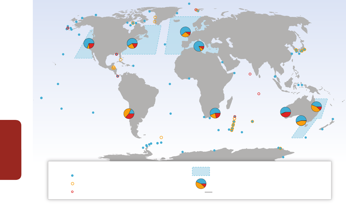
Cross-Chapter Box
Observed Global Responses of Marine Biogeography, Abundance, and Phenology to Climate Change
124
MB
The distributions of benthic, pelagic, and demersal species and communities have shifted by up to a thousand kilometers, although the
range shifts have not been uniform across taxonomic groups or ocean regions (Sections 6.3.2, 30.5) (robust evidence, high agreement, high
confidence). Overall, leading range edges expanded in a poleward direction at 72.0 ± 13.5 km per decade and trailing edges contracted in a
poleward direction at 15.8 ± 8.7 km per decade (Figure MB-2), revealing much higher current rates of migration than the potential maximum
rates reported for terrestrial species (Figure 4-6) despite slower warming of the ocean than land surface (WGI Section 3.2).
Poleward distribution shifts have resulted in increased species richness in mid- to high-latitude regions (Hiddink and ter Hofstede, 2008) and
changing community structure (Simpson et al., 2011; see also Section 28.2.2). Increases in warm-water components of communities concurrent
with regional warming have been observed in mid- to high-latitude ocean regions including the Bering Sea, Barents Sea, Nordic Sea, North
Sea, and Tasman Sea (Box 6.1; Section 30.5). Observed changes in species composition of catches from 1970–2006 that are partly attributed to
long-term ocean warming suggest increasing dominance of warmer water species in subtropical and higher latitude regions, and reduction in
abundance of subtropical species in equatorial waters (Cheung et al., 2013), with implications for fisheries (Sections 6.5, 7.4.2, 30.6.2.1).
The magnitude and direction of distribution shifts can be related to temperature velocities (i.e., the speed and direction at which isotherms
propagate across the ocean’s surface (Section 30.3.1.1; Burrows et al., 2011). Pinsky et al. (2013) showed that shifts in both latitude and depth
of benthic fish and crustaceans could be explained by climate velocity with remarkable accuracy, using a database of 128 million individuals
across 360 marine taxa from surveys of North American coastal waters conducted over 1968–2011. Poloczanska et al. (2013) found that
faster distribution shifts generally occur in regions of highest surface temperature velocity, such as the North Sea and sub-Arctic Pacific Ocean.
Observed marine species shifts, since approximately the 1950s, have generally been able to track observed velocities (Figure MB-3), with
phyto- and zooplankton distribution shifts vastly exceeding climate velocities observed over most of the ocean surface, but with considerable
variability within and among taxonomic groups (Poloczanska et al., 2013).
45
11
23
Change consistent with climate change
Type of observed change
No change
Change not consistent with climate change
222
221
772
42
41
132
Regions with large numbers of observations
Proportion of observed changes
Total number of observations within each region / locality41
Figure MB-1
| 1735 observed responses to climate change from 208 single- and multi-species studies. Data shown include changes that are attributed (at least partly) to
climate change (blue), changes that are inconsistent with climate change (red), and no change (orange). Each circle represents the center of a study area. Where points fall on
land, it is because they are centroids of distributions that surround an island or peninsula. Studies encompass areas from single sites (e.g., seabird breeding colony) to large
ocean regions (e.g., continuous plankton recorder surveys in north-east Atlantic). For regions (indicated by blue shading) and localities with large numbers of observations, pie
charts summarize the relative proportions of the three types of observed changes (consistent with climate change, inconsistent with climate change, and no change) in those
regions or localities. The numbers indicate the total observations within each region or locality. Note: 57% of the studies included were published since AR4. (From Poloczanska
et al., 2013).
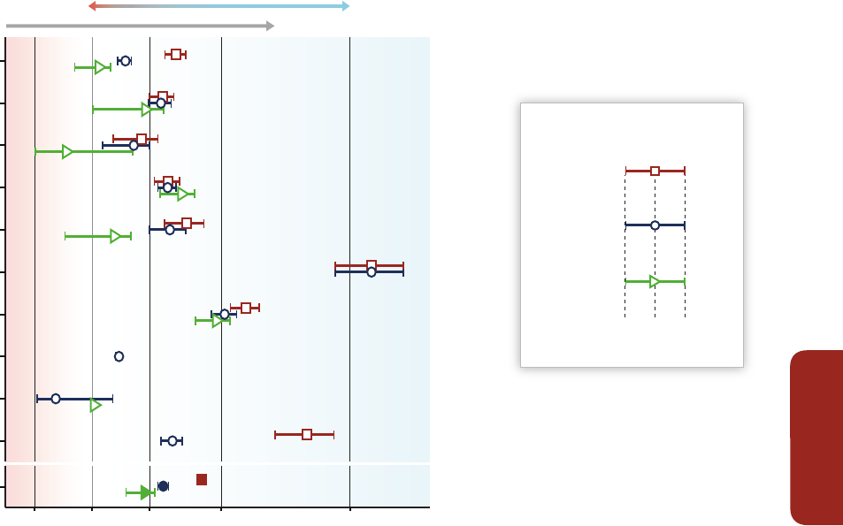
MB
Observed Global Responses of Marine Biogeography, Abundance, and Phenology to Climate Change
Cross-Chapter Box
125
Biogeographic shifts are also influenced by other factors such as currents, nutrient and stratification changes, light levels, sea ice, species’
interactions, habitat availability and fishing, some of which can be independently influenced by climate change (Section 6.3). Rate and pattern
of biogeographic shifts in sedentary organisms and benthic macroalgae are complicated by the influence of local dynamics and topographic
features (islands, channels, coastal lagoons, e.g., of the Mediterranean (Bianchi, 2007), coastal upwelling e.g., (Lima et al., 2007)). Geographical
barriers constrain range shifts and may cause a loss of endemic species (Ben Rais Lasram et al., 2010), with associated niches filled by alien
species, either naturally migrating or artificially introduced (Philippart et al., 2011).
Whether marine species can continue to keep pace as rates of warming, hence climate velocities, increase (Figure MB-3b) is a key uncertainty.
Climate velocities on land are expected to outpace the ability of many terrestrial species to track climate velocities this century (Section 4.3.2.5;
Figure 4-6). For marine species, the observed rates of shift are generally much faster than those for land species, particularly for primary
producers and lower trophic levels (Poloczanska et al., 2013). Phyto- and zooplankton communities (excluding larval fish) have extended
distributions at remarkable rates (Figure MB-3b), such as in the Northeast Atlantic (Section 30.5.1) with implications for marine food webs.
Geographical range shifts and depth distribution vary between coexisting marine species (Genner et al., 2004; Perry et al., 2005; Simpson et
al., 2011) as a consequence of the width of species-specific thermal windows and associated vulnerabilities (Figure 6-5). Warming therefore
causes differential changes in growth, reproductive success, larval output, early juvenile survival, and recruitment, implying shifts in the relative
performance of animal species and, thus, their competitiveness (Pörtner and Farrell, 2008; Figure 6-7A). Such effects may underlie abundance
losses or local extinctions, “regime shifts” between coexisting species, or critical mismatches between predator and prey organisms, resulting
in changes in local and regional species richness, abundance, community composition, productivity, energy flows, and invasion resistance.
Even among Antarctic stenotherms, differences in biological responses related to mode of life, phylogeny and associated metabolic capacities
exist (Section 6.3.1.4). As a consequence, marine ecosystem functions may be substantially reorganized at the regional scale, potentially
triggering a range of cascading effects (Hoegh-Guldberg and Bruno, 2010). A focus on understanding the mechanisms underpinning the nature
and magnitude of responses of marine organisms to climate change can help forecast impacts and the associated costs to society as well as
facilitate adaptive management strategies formitigating these impacts (Sections 6.3, 6.4).
Cooler watersWarmer waters
11
111
3
3
29
9
111
359
14
90
76
18
20
2
36
46
9
16
29
9
7
13
4
2
6
9
3
106
Distribution shift (km per decade)
–20 200 100 400
Benthic algae
Benthic cnidarians
Benthic mollusks
Benthic crustacea
Benthic invertebrates
(other)
Phytoplankton
Zooplankton
Larval bony fishes
Non-bony fishes
Bony fishes
All taxa
Number of
observations
Mean Standard
error
Standard
error
Direction of shift consistent with climate change (warming)
Distribution shifts towards:
Rates of change in
distribution measured at
leading edges
trailing edges
regardless of
range location
Figure MB-2 |
Rates of change in distribution (kilometers per decade) for marine taxonomic groups, measured at the leading edges (red) and trailing edges (green). Average
distribution shifts were calculated using all data, regardless of range location, and are in dark blue. Distribution shifts have been square-root transformed; standard errors may be
asymmetric as a result. Positive distribution changes are consistent with warming (into previously cooler waters, generally poleward). Means ± standard error are shown, along
with number of observations. Non-bony fishes include sharks, rays, lampreys, and hagfish. (From Poloczanska et al., 2013).
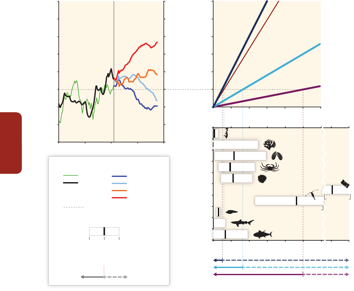
Cross-Chapter Box
Observed Global Responses of Marine Biogeography, Abundance, and Phenology to Climate Change
126
MB
Slow areas
Global median
Fast areas
Figure MB-3 |
(a) Rate of climate change for the ocean (sea surface temperature (SST) °C yr
-1
). (b) Corresponding climate velocities for the ocean and median velocity from land
(adapted from Burrows et al.
, 2011). (c) Observed rates of displacement of marine taxonomic groups based on observations over 1900–2010. The dotted bands give an example
of interpretation. Rates of climate change of 0.01 °C yr
-1
correspond to approximately 3.3 km yr
-1
median climate velocity in the ocean. When compared to observed rates of
displacement (c), many marine taxonomic groups have been able to track these velocities. For phytoplankton and zooplankton the rates of displacement greatly exceed median
climate velocity for the ocean and, for phytoplankton exceed velocities in fast areas of the ocean approximately 10.0 km yr
-1
. All values are calculated for ocean surface with the
exclusion of polar seas (Figure 30-1a). (a) Observed rates of climate change for ocean SST (green line) are derived from the Hadley Centre Interpolated SST 1.1 (HadISST1.1)
data set, and all other rates are calculated based on the average of the Coupled Model Intercomparison Project Phase 5 (CMIP5) climate model ensembles (Table SM30-3) for the
historical period and for the future based on the four Representative Concentration Pathway (RCP) scenarios. Data were smoothed using a 20-year sliding window. (b) Median
climate velocity over the global ocean surface (light blue line; excluding polar seas) calculated from HadSST1.1 data set over 1960–2009 using the methods of Burrows et al.
(2011). Median velocities representative of ocean regions of slow velocities such as the Pacific subtropical gyre (dark blue line) and of high velocities such as the Coral Triangle or
the North Sea (purple line) shown. Median rates over global land surface (red line) over 1960–2009 calculated using Climate Research Unit data set CRU TS3.1. Figure 30-3
shows climate velocities over the ocean surface calculated over 1960–2009. (c) Rates of displacement for marine taxonomic groups estimated by Poloczanska et al. (2013) using
published studies. Note the displacement rates for phytoplankton exceed the axis, so values are given.
0 2 4 6 8 10 12
0 2 4 6 8 10 4240
4240
12
0 2 4 6 8 10
55.0
15.7
35.8
12
Historical Projected
(a) Climate change scenarios
(km yr
–1
)
(km yr
–1
)
Rate of climate change for the ocean (sea surface temperature °C yr
–1
)
(°C yr
–1
)
Observed
Historical
RCP2.6
RCP4.5
RCP6.0
RCP8.5
−0.02
−0.01
0.00
0.01
0.02
0.05
0.04
0.03
0.06
0.00
0.01
0.02
0.05
0.04
0.03
0.06
0.00
0.01
0.02
0.05
0.04
0.03
0.06
1900 1950 2000 2050 2100
Lower bound
(25th percentile)
Upper bound
(75th percentile)
Estimated speed at which species group has moved
example of interpretation
Median
Unable to keep up Able to keep up
(c) Species displacement rates (required to track climate velocity)
(a) Rate of climate change
(c) Species displacement rates
(b) Estimate of climate velocity to determine rate of displacement
Land global median
Ocean slow areas
(e.g., subtropical gyres)
Ocean global median
Ocean fast areas
(e.g., equatorial and high latitudes)
Benthic algae
Benthic cnidarians
Benthic mollusks
Benthic crustacea
Other benthic
invertebrates
Phytoplankton
Zooplankton
Larval bony fishes
Non-bony fishes
Bony fishes

MB
Observed Global Responses of Marine Biogeography, Abundance, and Phenology to Climate Change
Cross-Chapter Box
127
Ben Rais Lasram, F., F. Guilhaumon, C. Albouy, S. Somot, W. Thuiller, and D. Mouillot, 2010: The Mediterranean Sea as a ‘cul-de-sac’ for endemic fishes facing climate
change. Global Change Biology, 16, 3233-3245.
Bianchi, C.N., 2007: Biodiversity issues for the forthcoming Mediterranean Sea. Hydrobiologia, 580, 7-21.
Burrows, M.T., D. S. Schoeman, L.B. Buckley, P.J. Moore, E.S. Poloczanska, K. Brander, K, C.J. Brown, J.F. Bruno, C.M. Duarte, B.S. Halpern, J. Holding, C.V. Kappel, W.
Kiessling, M.I. O’Connor, J.M. Pandolfi, C. Parmesan, F. Schwing, W.J. Sydeman, and A.J. Richardson, 2011: The pace of shifting climate in marine and terrestrial
ecosystems. Science, 334, 652-655.
Cheung, W.W.L., R. Watson, and D. Pauly, 2013: Signature of ocean warming in global fisheries catch. Nature, 497(7449), 365-368.
Genner, M.J., D.W. Sims, V.J. Wearmouth, E.J. Southall, A.J. Southward, P.A. Henderson, and S.J. Hawkins, 2004: Regional climatic warming drives long-term community
changes of British marine fish. Proceedings of the Royal Society B, 271(1539), 655-661.
Hiddink, J.G. and R. ter Hofstede, 2008: Climate induced increases in species richness of marine fishes. Global Change Biology, 14, 453-460.
Hoegh-Guldberg, O. and J.F. Bruno, 2010: The impact of climate change on the world’s marine ecosystems. Science, 328, 1523-1528.
Lima, F.P., P.A. Ribeiro, N. Queiroz, S.J. Hawkins, and A.M. Santos, 2007: Do distributional shifts of northern and southern species of algae match the warming pattern?
Global Change Biology, 13, 2592-2604.
Perry, A.L., P.J. Low, J.R. Ellis, and J.D. Reynolds, 2005: Climate change and distribution shifts in marine fishes. Science, 308(5730), 1912-1915.
Philippart, C.J.M., R. Anadon, R. Danovaro, J.W. Dippner, K.F. Drinkwater, S.J. Hawkins, T. Oguz, G. O’Sullivan, and P.C. Reid, 2011: Impacts of climate change on European
marine ecosystems: observations, expectations and indicators. Journal of Experimental Marine Biology and Ecology, 400, 52-69.
Pinksy, M.L., B. Worm, M.J. Fogarty, J.L. Sarmiento, and S.A. Levin, 2013: Marine taxa track local climate velocities. Science, 341, 1239-1242.
Pörtner, H.O. and A.P. Farrell, 2008: Physiology and climate change. Science, 322(5902), 690-692.
Poloczanska, E.S., C.J. Brown, W.J. Sydeman, W. Kiessling, D.S. Schoeman, P.J. Moore, K. Brander, J.F. Bruno, L.B. Buckley, M.T. Burrows, C.M. Duarte, B.S. Halpern, J.
Holding, C.V. Kappel, M.I. O’Connor, J.M. Pandolfi, C. Parmesan, F. Schwing, S.A.Thompson, and A.J. Richardson, 2013: Global imprint of climate change on marine
life. Nature Climate Change, 3, 919-925.
Simpson, S.D., S. Jennings, M.P. Johnson, J.L. Blanchard, P.J. Schon, D.W. Sims, and M.J. Genner, 2011: Continental shelf-wide response of a fish assemblage to rapid
warming of the sea. Current Biology, 21, 1565-1570.
References
Poloczanska, E.S., O. Hoegh-Guldberg, W. Cheung, H.-O. Pörtner, and M. Burrows, 2014: Cross-chapter box on observed global responses of marine biogeogra-
phy, abundance, and phenology to climate change. In: Climate Change 2014: Impacts, Adaptation, and Vulnerability. Part A: Global and Sectoral Aspects.
Contribution of Working Group II to the Fifth Assessment Report of the Intergovernmental Panel on Climate Change [Field, C.B., V.R. Barros, D.J. Dokken, K.J.
Mach, M.D. Mastrandrea, T.E. Bilir, M. Chatterjee, K.L. Ebi, Y.O. Estrada, R.C. Genova, B. Girma, E.S. Kissel, A.N. Levy, S. MacCracken, P.R. Mastrandrea, and
L.L. White (eds.)]. Cambridge University Press, Cambridge, United Kingdom and New York, NY, USA, pp. 123-127.
This cross-chapter box should be cited as:

Ocean Acidification
Jean-Pierre Gattuso (France), Peter G. Brewer (USA), Ove Hoegh-Guldberg (Australia), Joan A.
Kleypas (USA), Hans-Otto Pörtner (Germany), Daniela N. Schmidt (UK)
OA
129
Anthropogenic ocean acidification and global warming share the same primary cause, which is
the increase of atmospheric CO
2
(Figure OA-1A; WGI, Section 2.2.1). Eutrophication, loss of sea ice,
upwelling and deposition of atmospheric nitrogen and sulfur all exacerbate ocean acidification
locally (Sections 5.3.3.6, 6.1.1, 30.3.2.2).
Chemistry and Projections
The fundamental chemistry of ocean acidification is well understood (robust evidence, high
agreement). Increasing atmospheric concentrations of CO
2
result in an increased flux of CO
2
into a
mildly alkaline ocean, resulting in a reduction in pH, carbonate ion concentration, and the capacity
of seawater to buffer changes in its chemistry (very high confidence). The changing chemistry of
the surface layers of the open ocean can be projected at the global scale with high accuracy using
projections of atmospheric CO
2
levels (Figure CC-OA-1B). Observations of changing upper ocean
CO
2
chemistry over time support this linkage (WGI Table 3.2 and Figure 3.18; Figures 30-8, 30-9).
Projected changes in open ocean, surface water chemistry for the year 2100 based on representative
concentration pathways (WGI, Figure 6.28) compared to pre-industrial values range from a pH
change of –0.14 units with Representative Concentration Pathway (RCP)2.6 (421 ppm CO
2
, +1°C,
22% reduction of carbonate ion concentration) to a pH change of –0.43 units with RCP8.5 (936
ppm CO
2
, +3.7ºC, 56% reduction of carbonate ion concentration). Projections of regional changes,
especially in the highly complex coastal systems (Sections 5.3.3.5, 30.3.2.2), in polar regions (WGI
Section 6.4.4), and at depth are more difficult but generally follow similar trends.
Biological, Ecological, and Biogeochemical Impacts
Investigations of the effect of ocean acidification on marine organisms and ecosystems have a
relatively short history, recently analyzed in several meta-analyses (Sections 6.3.2.1, 6.3.5.1). A wide
range of sensitivities to projected rates of ocean acidification exists within and across diverse groups
of organisms, with a trend for greater sensitivity in early life stages (high confidence; Sections
5.4.2.2, 5.4.2.4, 6.3.2). A pattern of positive and negative impacts emerges (high confidence; Figure
OA-1C) but key uncertainties remain in our understanding of the impacts on organisms, life histories,
and ecosystems. Responses can be influenced, often exacerbated by other drivers, such as warming,
hypoxia, nutrient concentration, and light availability (high confidence; Sections 5.4.2.4, 6.3.5).
Growth and primary production are stimulated in seagrass and some phytoplankton (high
confidence; Sections 5.4.2.3, 6.3.2.2, 6.3.2.3, 30.5.6). Harmful algal blooms could become more
frequent (limited evidence, medium agreement). Ocean acidification may stimulate nitrogen fixation
(limited evidence, low agreement; 6.3.2.2). It decreases the rate of calcification of most, but not
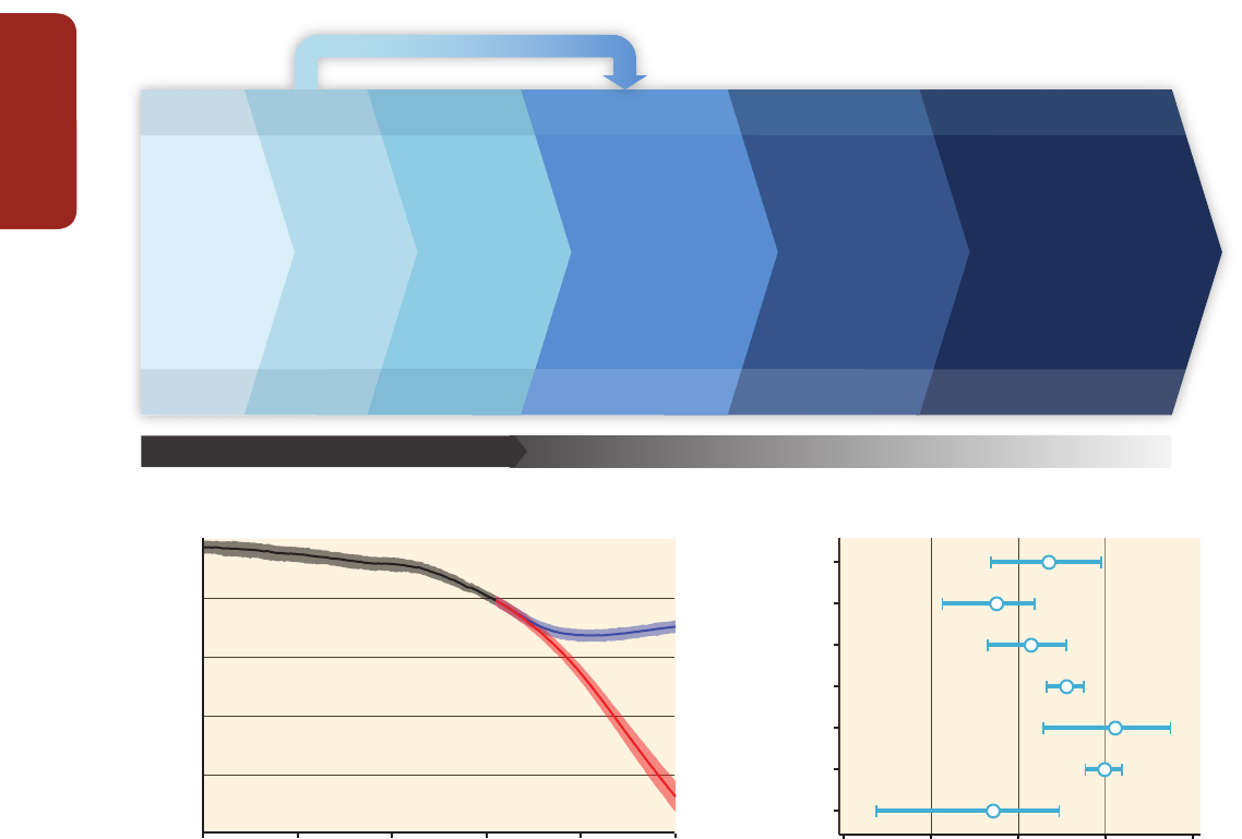
Cross-Chapter Box
Ocean Acidification
130
OA
all, sea floor calcifiers (medium agreement, robust evidence) such as reef-building corals (Box CC-CR), coralline algae, bivalves, and gastropods,
reducing the competitiveness with non-calcifiers (Sections 5.4.2.2, 5.4.2.4, 6.3.2.5). Ocean warming and acidification promote higher rates of
calcium carbonate dissolution resulting in the net dissolution of carbonate sediments and frameworks and loss of associated habitat (medium
confidence; 5.4.2.4, 6.3.2.5, 6.3.5.4). Some corals and temperate fishes experience disturbances to behavior, navigation, and their ability to tell
conspecifics from predators (Section 6.3.2.4). However, there is no evidence for these effects to persist on evolutionary time scales in the few
groups analyzed (Section 6.3.2).
Some phytoplankton and molluscs displayed adaptation to ocean acidification in long-term experiments (limited evidence, medium agreement;
Section 6.3.2.1), indicating that the long-term responses could be less than responses obtained in short-term experiments. However, mass
extinctions in Earth history occurred during much slower rates of ocean acidification, combined with other drivers changing, suggesting that
evolutionary rates are not fast enough for sensitive animals and plants to adapt to the projected rate of future change (medium confidence;
Section 6.1.2).
Projections of ocean acidification effects at the ecosystem level are made difficult by the diversity of species-level responses. Differential
sensitivities and associated shifts in performance and distribution will change predator–prey relationships and competitive interactions (Sections
RCP8.5
RCP2.6
Historical
7.7
7.8
7.9
8.0
8.1
8.2
pH (total scale)
1850 1900 1950 2000 2050 2100
Burning of fossil
fuels, cement
manufacture,
and land use
change
(WGI 2.2.1)
(WGI 3.8.2;
WGII 5.3.3, 30.3.2)
(WGII 5.4.2. 6.3.2, 30.5)
(WGII 5.4.2.2, 5.4.2.4,
30.6.2, Box CC-CR)
(WGII 30.6.4, 30.7.1)
Increase in
atmospheric
CO
2
High certainty Low certainty
• Increased CO
2
,
bicarbonate
ions, and acidity
• Decreased
carbonate ions
and pH
• Reduced shell and
skeleton production
• Changes in
assemblages, food
webs, and ecosystems
• Biodiversity loss
• Changes in biogas
production and
feedback to climate
• Fisheries,
aquaculture, and
food security
• Coastal protection
• Tourism
• Climate regulation
• Carbon storage
• UN Framework Convention on
Climate Change: Conference
of the Parties, IPCC,
Conference on Sustainable
Development (Rio+20)
• Convention on Biological
Diversity
• Geoengineering
• Regional and local acts, laws,
and policies to reduce other
stresses
(a)
(b)
–0.75 –0.50 –0.25 0 0.25
Mean effect size (lnRR)Year
Abundance
Calcification
Development
Growth
Metabolism
Photosynthesis
Survival
(72)
(110)
(24)
(173)
(32)
(82)
(69)
(c)
Ocean acidification
Atmospheric
change
Changes to organisms
and ecosystems
Socioeconomic impacts
Ocean warming and deoxgenation
relevant sections
(WGI 6.3.2)
Policy options for actionDriver
Figure OA-1 |
(a) Overview of the chemical, biological, and socio-economic impacts of ocean acidification and of policy options (adapted from Turley and Gattuso, 2012). (b) Multi-model
simulated time series of global mean ocean surface pH (on the total scale) from Coupled Model Intercomparison Project Phase 5 (
CMIP5) climate model simulations from 1850 to 2100.
Projections are shown for emission scenarios Representative Concentration Pathway (RCP)2.6 (blue) and RCP8.5 (red) for the multi-model mean (solid lines) and range across the
distribution of individual model simulations (shading). Black (gray shading) is the modeled historical evolution using historical reconstructed forcings. The models that are included are those
from CMIP5 that simulate the global carbon cycle while being driven by prescribed atmospheric CO
2
concentrations (WGI AR5 Figures SPM.7 and TS.20). (c) Effect of near-future
acidification (
seawater pH reduction of ≤0.5 units) on major response variables estimated using weighted random effects meta-analyses, with the exception of survival, which is not
weighted (Kroeker et al., 2013). The log-transformed response ratio (lnRR) is the ratio of the mean effect in the acidification treatment to the mean effect in a control group. It indicates
which process is most uniformly affected by ocean acidification, but large variability exists between species. Significance is determined when the 95% bootstrapped confidence interval
does not cross zero. The number of experiments used in the analyses is shown in parentheses. The * denotes a statistically significant effect.
*
*
*
*
*

OA
Ocean Acidification
Cross-Chapter Box
131
6.3.2.5, 6.3.5, 6.3.6), which could impact food webs and higher trophic levels (limited evidence, high agreement). Natural analogues at CO
2
vents
indicate decreased species diversity, biomass, and trophic complexity of communities (Box CC-CR; Sections 5.4.2.3, 6.3.2.5, 30.3.2.2, 30.5). Shifts in
community structure have also been documented in regions with rapidly declining pH (Section 5.4.2.2).
Owing to an incomplete understanding of species-specific responses and trophic interactions, the effect of ocean acidification on global
biogeochemical cycles is not well understood (limited evidence, low agreement) and represents an important knowledge gap. The additive,
synergistic, or antagonistic interactions of factors such as temperature, concentrations of oxygen and nutrients, and light are not sufficiently
investigated yet.
Risks, Socioeconomic Impacts, and Costs
The risks of ocean acidification to marine organisms, ecosystems, and ultimately to human societies, include both the probability that ocean
acidification will affect fundamental physiological and ecological processes of organisms (Section 6.3.2.1), and the magnitude of the resulting
impacts on ecosystems and the ecosystem services they provide to society (Box 19-2). For example, ocean acidification under RCP4.5 to RCP8.5
will impact formation and maintenance of coral reefs (high confidence; Box CC-CR, Section 5.4.2.4) and the goods and services that they provide
such as fisheries, tourism, and coastal protection (limited evidence, high agreement; Box CC-CR; Sections 6.4.1.1,19.5.2, 27.3.3, 30.5, 30.6). Ocean
acidification poses many other potential risks, but these cannot yet be quantitatively assessed because of the small number of studies available,
particularly on the magnitude of the ecological and socioeconomic impacts (Section 19.5.2).
Global estimates of observed or projected economic costs of ocean acidification do not exist. The largest uncertainty is how the impacts on lower
trophic levels will propagate through the food webs and to top predators. However, there are a number of instructive examples that illustrate
the magnitude of potential impacts of ocean acidification. A decrease of the production of commercially exploited shelled molluscs (Section
6.4.1.1) would result in a reduction of USA production of 3 to 13% according to the Special Report on Emission Scenarios (SRES) A1FI emission
scenario (low confidence). The global cost of production loss of molluscs could be more than US$100 billion by 2100 (limited evidence, medium
agreement). Models suggest that ocean acidification will generally reduce fish biomass and catch (low confidence) and that complex additive,
antagonistic, and/or synergistic interactions will occur with other environmental (warming) and human (fisheries management) factors (Section
6.4.1.1). The annual economic damage of ocean-acidification–induced coral reef loss by 2100 has been estimated, in 2012, to be US$870 and 528
billion, respectively for the A1 and B2 SRES emission scenarios (low confidence; Section 6.4.1). Although this number is small compared to global
gross domestic product (GDP), it can represent a very large GDP loss for the economies of many coastal regions or small islands that rely on the
ecological goods and services of coral reefs (Sections 25.7.5, 29.3.1.2).
Mitigation and Adaptation
Successful management of the impacts of ocean acidification includes two approaches: mitigation of the source of the problem (i.e., reduce
anthropogenic emissions of CO
2
) and/or adaptation by reducing the consequences of past and future ocean acidification (Section 6.4.2.1).
Mitigation of ocean acidification through reduction of atmospheric CO
2
is the most effective and the least risky method to limit ocean acidification
and its impacts (Section 6.4.2.1). Climate geoengineering techniques based on solar radiation management will not abate ocean acidification
and could increase it under some circumstances (Section 6.4.2.2). Geoengineering techniques to remove CO
2
from the atmosphere could directly
address the problem but are very costly and may be limited by the lack of CO
2
storage capacity (Section 6.4.2.2). In addition, some ocean-
based approaches, such as iron fertilization, would only relocate ocean acidification from the upper ocean to the ocean interior, with potential
ramifications on deep water oxygen levels (Sections 6.4.2.2, 30.3.2.3, 30.5.7). A low-regret approach, with relatively limited effectiveness, is to
limit the number and the magnitude of drivers other than CO
2
, such as nutrient pollution (Section 6.4.2.1). Mitigation of ocean acidification at
the local level could involve the reduction of anthropogenic inputs of nutrients and organic matter in the coastal ocean (Section 5.3.4.2). Some
adaptation strategies include drawing water for aquaculture from local watersheds only when pH is in the right range, selecting for less sensitive
species or strains, or relocating industries elsewhere (Section 6.4.2.1).
Kroeker, K., R.C. Kordas, A. Ryan, I. Hendriks, L. Ramajo, G. Singh, C. Duarte, and J.-P. Gattuso, 2013: Impacts of ocean acidification on marine organisms: quantifying
sensitivities and interaction with warming. Global Change Biology, 19, 1884-1896.
Turley, C. and J.-P. Gattuso, 2012: Future biological and ecosystem impacts of ocean acidification and their socioeconomic-policy implications. Current Opinion in
Environmental Sustainability, 4, 278-286.
References
Gattuso, J.-P., P.G. Brewer, O. Hoegh-Guldberg, J.A. Kleypas, H.-O. Pörtner, and D.N. Schmidt, 2014: Cross-chapter box on ocean acidification. In: Climate Change
2014: Impacts, Adaptation, and Vulnerability. Part A: Global and Sectoral Aspects. Contribution of Working Group II to the Fifth Assessment Report of the
Intergovernmental Panel on Climate Change [Field, C.B., V.R. Barros, D.J. Dokken, K.J. Mach, M.D. Mastrandrea, T.E. Bilir, M. Chatterjee, K.L. Ebi, Y.O. Estrada,
R.C. Genova, B. Girma, E.S. Kissel, A.N. Levy, S. MacCracken, P.R. Mastrandrea, and L.L. White (eds.)]. Cambridge University Press, Cambridge, United King-
dom and New York, NY, USA, pp. 129-131.
This cross-chapter box should be cited as:

Net Primary Production in
the Ocean
Philip W. Boyd (New Zealand), Svein Sundby (Norway), Hans-Otto Pörtner (Germany)
PP
133
Net Primary Production (NPP) is the rate of photosynthetic carbon fixation minus the fraction of
fixed carbon used for cellular respiration and maintenance by autotrophic planktonic microbes
and benthic plants (Sections 6.2.1, 6.3.1). Environmental drivers of NPP include light, nutrients,
micronutrients, CO
2
, and temperature (Figure PP-1a). These drivers, in turn, are influenced by
oceanic and atmospheric processes, including cloud cover; sea ice extent; mixing by winds, waves,
and currents; convection; density stratification; and various forms of upwelling induced by eddies,
frontal activity, and boundary currents. Temperature has multiple roles as it influences rates
of phytoplankton physiology and heterotrophic bacterial recycling of nutrients, in addition to
stratification of the water column and sea ice extent (Figure PP-1a). Climate change is projected
to strongly impact NPP through a multitude of ways that depend on the regional and local
physical settings (WGI AR5, Chapter 3), and on ecosystem structure and functioning (medium
confidence; Sections 6.3.4, 6.5.1). The influence of environmental drivers on NPP causes as much
as a 10-fold variation in regional productivity with nutrient-poor subtropical waters and light-
limited Arctic waters at the lower range and productive upwelling regions and highly eutrophic
coastal regions at the upper range (Figure PP-1b).
The oceans currently provide ~50 × 10
15
g C yr
–1
, or about half of global NPP (Field et al., 1998).
Global estimates of NPP are obtained mainly from satellite remote sensing (Section 6.1.2),
which provides unprecedented spatial and temporal coverage, and may be validated regionally
against oceanic measurements. Observations reveal significant changes in rates of NPP when
environmental controls are altered by episodic natural perturbations, such as volcanic eruptions
enhancing iron supply, as observed in high-nitrate low-chlorophyll waters of the Northeast Pacific
(Hamme et al., 2010). Climate variability can drive pronounced changes in NPP (Chavez et al.,
2011), such as from El Niño to La Niña transitions in Equatorial Pacific, when vertical nutrient and
trace element supply are enhanced (Chavez et al., 1999).
Multi-year time series records of NPP have been used to assess spatial trends in NPP in recent
decades. Behrenfeld et al. (2006), using satellite data, reported a prolonged and sustained global
NPP decrease of 190 × 10
12
g C yr
–1
, for the period 1999–2005—an annual reduction of 0.57%
of global NPP. In contrast, a time series of directly measured NPP between 1988 and 2007 by
Saba et al. (2010) (i.e., in situ incubations using the radiotracer
14
C-bicarbonate) revealed an
increase (2% yr
–1
) in NPP for two low-latitude open ocean sites. This discrepancy between in situ
and remotely sensed NPP trends points to uncertainties in either the methodology used and/
or the extent to which discrete sites are representative of oceanic provinces (Saba et al., 2010,
2011). Modeling studies have subsequently revealed that the <15-year archive of satellite-
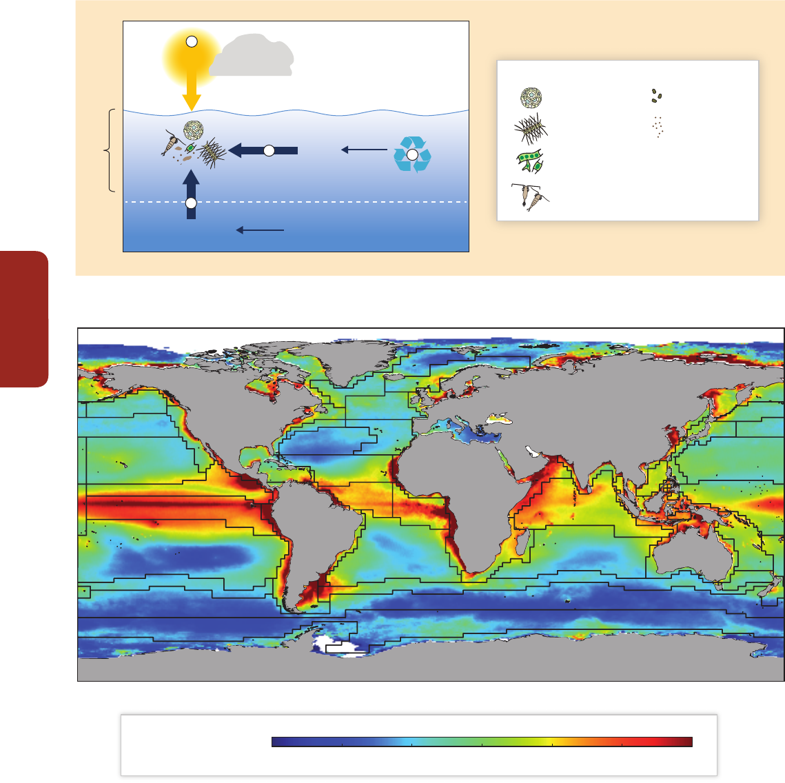
Cross-Chapter Box
Net Primary Production in the Ocean
134
PP
Nutrient
recycling
•
Nutrients
•
Trace metals
Euphotic zone (0–100 m)
•
Upwelling
•
Vertical mixing
•
Stratification
(a)
Light
•
Zooplankton
•
Microbes
NPP (g C m
–
² y
–
¹)
300 250 200 150 100 50 0
(b)
Latitude
Season
Cloud cover
Figure PP-1 |
(a) Environmental factors controlling Net Primary Production (NPP). NPP is controlled mainly by three basic processes: (1) light conditions in the surface ocean, that
is, the photic zone where photosynthesis occurs; (2) upward flux of nutrients and micronutrients from underlying waters into the photic zone, and (3) regeneration of nutrients and
micronutrients via the breakdown and recycling of organic material before it sinks out of the photic zone. All three processes are influenced by physical, chemical, and biological
processes and vary across regional ecosystems. In addition, water temperature strongly influences the upper rate of photosynthesis for cells that are resource-replete. Predictions of
alteration of primary productivity under climate change depend on correct parameterizations and simulations of each of these variables and processes for each region. (b) Annual
composite map of global areal NPP rates (derived from Moderate Resolution Imaging Spectroradiometer (MODIS) Aqua satellite climatology from 2003–2012; NPP was calculated
with the Carbon-based Productivity Model (CbPM; Westberry et al., 2008)). Overlaid is a grid of (thin black lines) that represent 51 distinct global ocean biogeographical provinces
(after Longhurst, 1998 and based on Boyd and Doney, 2002). The characteristics and boundaries of each province are primarily set by the underlying regional ocean physics and
chemistry. White areas = no data. (Figure courtesy of Toby Westberry (OSU) and Ivan Lima (WHOI), satellite data courtesy of NASA Ocean Biology Processing Group.)
1
3
3
2
Copepod pellets
Microzooplankton
mini-pellets
Particles
Coccolithophorids
Diatoms
Other
Phytoplankton
Copepods
Plankton
Temperature

PP
Net Primary Production in the Ocean
Cross-Chapter Box
135
Arrigo, K.R. and G.L. van Dijken, 2011: Secular trends in Arctic Ocean net primary production. Journal of Geophysical Research, 116(C9), C09011,
doi:10.1029/2011JC007151.
Beaulieu, C., S.A. Henson, J.L. Sarmiento, J.P. Dunne, S.C. Doney, R.R. Rykaczewski, and L. Bopp, 2013: Factors challenging our ability to detect long-term trends in ocean
chlorophyll. Biogeosciences, 10(4), 2711-2724.
Behrenfeld, M.J., R.T. O’Malley, D.A. Siegel, C.R. McClain, J.L. Sarmiento, G.C. Feldman, A.J. Milligan, P.G. Falkowski, R.M. Letelier, and E.S. Boss, 2006: Climate-driven
trends in contemporary ocean productivity. Nature, 444(7120), 752-755.
Bopp, L., L. Resplandy, J.C. Orr, S.C. Doney, J.P. Dunne, M. Gehlen, P. Halloran, C. Heinze, T. Ilyina, R. Séférian, J. Tijiputra, and M. Vichi, 2013: Multiple stressors of ocean
ecosystems in the 21st century: projections with CMIP5 models. Biogeosciences, 10, 6225-6245.
Boyce, D.G., M.R. Lewis, and B. Worm, 2010: Global phytoplankton decline over the past century. Nature, 466(7306), 591-596.
Boyd, P.W. and S.C. Doney, 2002: Modelling regional responses by marine pelagic ecosystems to global climate change. Geophysical Research Letters, 29(16), 53-1–53-4,
doi:10.1029/2001GL014130.
Boyd, P.W., R. Strzepek, F.X. Fu, and D.A. Hutchins, 2010: Environmental control of open-ocean phytoplankton groups: now and in the future. Limnology and
Oceanography, 55(3), 1353-1376.
Chavez, F.P., P.G. Strutton, C.E. Friederich, R.A. Feely, G.C. Feldman, D.C. Foley, and M.J. McPhaden, 1999: Biological and chemical response of the equatorial Pacific Ocean
to the 1997-98 El Niño. Science, 286(5447), 2126-2131.
References
derived NPP is insufficient to distinguish climate-change mediated shifts in NPP from those driven by natural climate variability (Henson et al.,
2010; Beaulieu et al., 2013). Although multi-decadal, the available time series of oceanic NPP measurements are also not of sufficient duration
relative to the time scales of longer-term climate variability modes as for example Atlantic Multi-decadal Oscillation (AMO), with periodicity of
60-70 years, Figure 6-1). Recent attempts to synthesize longer (i.e., centennial) records of chlorophyll as a proxy for phytoplankton stocks (e.g.,
Boyce et al., 2010) have been criticized for relying on questionable linkages between different proxies for chlorophyll over a century of records
(e.g., Rykaczewski and Dunne, 2011).
Models in which projected climate change alters the environmental drivers of NPP provide estimates of spatial changes and of the rate of
change of NPP. For example, four global coupled climate–ocean biogeochemical Earth System Models (WGI AR5 Chapter 6) projected an
increase in NPP at high latitudes as a result of alleviation of light and temperature limitation of NPP, particularly in the high-latitude biomes
(Steinacher et al., 2010). However, this regional increase in NPP was more than offset by decreases in NPP at lower latitudes and at mid-
latitudes due to the reduced input of macronutrients into the photic zone. The reduced mixed-layer depth and reduced rate of circulation may
cause a decrease in the flux of macronutrients to the euphotic zone (Figure 6-2). These changes to oceanic conditions result in a reduction in
global mean NPP by 2 to 13% by 2100 relative to 2000 under a high emission scenario (Polovina et al., 2011; SRES (Special Report on Emission
Scenarios) A2, between RCP6.0 and RCP8.5). This is consistent with a more recent analysis based on 10 Earth System Models (Bopp et al.,
2013), which project decreases in global NPP by 8.6 (±7.9), 3.9 (±5.7), 3.6 (±5.7), and 2.0 (±4.1) % in the 2090s relative to the 1990s, under
the scenarios RCP8.5, RCP6.0, RCP4.5, and RCP2.6, respectively. However, the magnitude of projected changes varies widely between models
(e.g., from 0 to 20% decrease in NPP globally under RCP 8.5). The various models show very large differences in NPP at regional scales (i.e.,
provinces, see Figure PP-1b).
Model projections had predicted a range of changes in global NPP from an increase (relative to preindustrial rates) of up to 8.1% under an
intermediate scenario (SRES A1B, similar to RCP6.0; Sarmiento et al., 2004; Schmittner et al., 2008) to a decrease of 2-20% under the SRES A2
emission scenario (Steinacher et al., 2010). These projections did not consider the potential contribution of primary production derived from
atmospheric nitrogen fixation in tropical and subtropical regions, favoured by increasing stratification and reduced nutrient inputs from mixing.
This mechanism is potentially important, although such episodic increases in nitrogen fixation are not sustainable without the presence of
excess phosphate (e.g., Moore et al., 2009; Boyd et al., 2010). This may lead to an underestimation of NPP (Mohr et al., 2010; Mulholland et al.,
2012; Wilson et al., 2012), however, the extent of such underestimation is unknown (Luo et al., 2012).
Care must be taken when comparing global, provincial (e.g., low-latitude waters, e.g., Behrenfeld et al., 2006) and regional trends in NPP
derived from observations, as some regions have additional local environmental influences such as enhanced density stratification of the upper
ocean from melting sea ice. For example, a longer phytoplankton growing season, due to more sea ice–free days, may have increased NPP
(based on a regionally validated time-series of satellite NPP) in Arctic waters (Arrigo and van Dijken, 2011) by an average of 8.1x10
12
g C yr
−1
between 1998 and 2009. Other regional trends in NPP are reported in Sections 30.5.1 to 30.5.6. In addition, although future model projections
of global NPP from different models (Steinacher et al., 2010; Bopp et al., 2013) are comparable, regional projections from each of the models
differ substantially. This raises concerns as to which aspect(s) of the different model NPP parameterizations are responsible for driving regional
differences in NPP, and moreover, how accurate model projections are of global NPP.
From a global perspective, open ocean NPP will decrease moderately by 2100 under both low- (SRES B1 or RCP4.5) and high-emission
scenarios (medium confidence; SRES A2 or RCPs 6.0, 8.5, Sections 6.3.4, 6.5.1), paralleled by an increase in NPP at high latitudes and
a decrease in the tropics (medium confidence). However, there is limited evidence and low agreement on the direction, magnitude and
differences of a change of NPP in various ocean regions and coastal waters projected by 2100 (low confidence).

Cross-Chapter Box
Net Primary Production in the Ocean
136
PP
Boyd, P.W., S. Sundby, and H.-O. Pörtner, 2014: Cross-chapter box on net primary production in the ocean. In: Climate Change 2014: Impacts, Adaptation, and
Vulnerability. Part A: Global and Sectoral Aspects. Contribution of Working Group II to the Fifth Assessment Report of the Intergovernmental Panel on
Climate Change [Field, C.B., V.R. Barros, D.J. Dokken, K.J. Mach, M.D. Mastrandrea, T.E. Bilir, M. Chatterjee, K.L. Ebi, Y.O. Estrada, R.C. Genova, B. Girma, E.S.
Kissel, A.N. Levy, S. MacCracken, P.R. Mastrandrea, and L.L. White (eds.)]. Cambridge University Press, Cambridge, United Kingdom and New York, NY, USA,
pp. 133-136.
Chavez, F.P., M. Messié, and J.T. Pennington, 2011: Marine primary production in relation to climate variability and change. Annual Review of Marine Science, 3(1), 227-
260.
Field, C.B., M.J. Behrenfeld, J.T. Randerson, and P. Falkowski, 1998: Primary production of the biosphere: integrating terrestrial and oceanic components. Science,
281(5374), 237-240.
Hamme, R.C., P.W. Webley, W.R. Crawford, F.A. Whitney, M.D. DeGrandpre, S.R. Emerson, C.C. Eriksen, K.E. Giesbrecht, J.F.R. Gower, M.T. Kavanaugh, M.A. Peña, C.L.
Sabine, S.D. Batten, L.A. Coogan, D.S. Grundle, and D. Lockwood, 2010: Volcanic ash fuels anomalous plankton bloom in subarctic northeast Pacific. Geophysical
Research Letters, 37(19), L19604, doi:10.1029/2010GL044629.
Henson, S.A., J.L. Sarmiento, J.P. Dunne, L. Bopp, I. Lima, S.C. Doney, J. John, and C. Beaulieu, 2010: Detection of anthropogenic climate change in satellite records of ocean
chlorophyll and productivity. Biogeosciences, 7(2), 621-640.
Longhurst, A.R., 1998: Ecological Geography of the Sea. Academic Press, San Diego, CA, USA, 560 pp.
Luo, Y.-W., S.C. Doney, L.A. Anderson, M. Benavides, I. Berman-Frank, A. Bode, S. Bonnet, K.H. Boström, D. Böttjer, D.G. Capone, E.J. Carpenter, Y.L. Chen, M.J. Church, J.E.
Dore, L.I. Falcón, A. Fernández, R.A. Foster, K. Furuya, F. Gómez, K. Gundersen, A.M. Hynes, D.M. Karl, S. Kitajima, R.J. Langlois, J. LaRoche, R.M. Letelier, E. Marañón,
D.J. McGillicuddy Jr., P.H. Moisander, C.M. Moore, B. Mouriño-Carballido, M.R. Mulholland, J.A. Needoba, K.M. Orcutt, A.J. Poulton, E. Rahav, P. Raimbault, A.P. Rees, L.
Riemann, T. Shiozaki, A. Subramaniam, T. Tyrrell, K.A. Turk-Kubo, M. Varela, T.A. Villareal, E.A. Webb, A.E. White, J. Wu, and J.P. Zehr, 2012: Database of diazotrophs in
global ocean: abundances, biomass and nitrogen fixation rates. Earth System Science Data, 4, 47-73, doi:10.5194/essd-4-47-2012.
Mohr, W., T. Großkopf, D.W.R. Wallace, and J. LaRoche, 2010: Methodological underestimation of oceanic nitrogen fixation rates. PLoS ONE, 5(9), e12583, doi:10.1371/
journal.pone.0012583.
Moore, C.M., M.M. Mills, E.P. Achterberg, R.J. Geider, J. LaRoche, M.I. Lucas, E.L. McDonagh, X. Pan, A.J. Poulton, M.J.A. Rijkenberg, D.J. Suggett, S.J. Ussher, and E.M.S.
Woodward, 2009: Large-scale distribution of Atlantic nitrogen fixation controlled by iron availability. Nature Geoscience, 2(12), 867-871.
Mulholland, M.R., P.W. Bernhardt, J.L. Blanco-Garcia, A. Mannino, K. Hyde, E. Mondragon, K. Turk, P.H. Moisander, and J.P. Zehr, 2012: Rates of dinitrogen fixation and the
abundance of diazotrophs in North American coastal waters between Cape Hatteras and Georges Bank. Limnology and Oceanography, 57(4), 1067-1083.
Polovina, J.J., J.P. Dunne, P.A. Woodworth, and E.A. Howell, 2011: Projected expansion of the subtropical biome and contraction of the temperate and equatorial upwelling
biomes in the North Pacific under global warming. ICES Journal of Marine Science, 68(6), 986-995.
Rykaczewski, R.R. and J.P. Dunne, 2011: A measured look at ocean chlorophyll trends. Nature, 472(7342), E5-E6, doi:10.1038/nature09952.
Saba, V.S., M.A.M. Friedrichs, M.-E. Carr, D. Antoine, R.A. Armstrong, I. Asanuma, O. Aumont, N.R. Bates, M.J. Behrenfeld, V. Bennington, L. Bopp, J. Bruggeman, E.T.
Buitenhuis, M.J. Church, A.M. Ciotti, S.C. Doney, M. Dowell, J. Dunne, S. Dutkiewicz, W. Gregg, N. Hoepffner, K.J.W. Hyde, J. Ishizaka, T. Kameda, D.M. Karl, I. Lima,
M.W. Lomas, J. Marra, G.A. McKinley, F. Mélin, J.K. Moore, A. Morel, J. O’Reilly, B. Salihoglu, M. Scardi, T.J. Smyth, S.L. Tang, J. Tjiputra, J. Uitz, M. Vichi, K. Waters, T.K.
Westberry, and A. Yool, 2010: Challenges of modeling depth-integrated marine primary productivity over multiple decades: a case study at BATS and HOT. Global
Biogeochemical Cycles, 24, GB3020, doi:10.1029/2009GB003655.
Saba, V.S., M.A.M. Friedrichs, D. Antoine, R.A. Armstrong, I. Asanuma, M.J. Behrenfeld, A.M. Ciotti, M. Dowell, N. Hoepffner, K.J.W. Hyde, J. Ishizaka, T. Kameda, J. Marra, F.
Mélin, A. Morel, J. O’Reilly, M. Scardi, W.O. Smith Jr., T.J. Smyth, S. Tang, J. Uitz, K. Waters, and T.K. Westberry, 2011: An evaluation of ocean color model estimates of
marine primary productivity in coastal and pelagic regions across the globe. Biogeosciences, 8(2), 489-503.
Sarmiento, J.L., R. Slater, R. Barber, L. Bopp, S.C. Doney, A.C. Hirst, J. Kleypas, R. Matear, U. Mikolajewicz, P. Monfray, V. Soldatov, S.A. Spall, and R. Stouffer, 2004: Response
of ocean ecosystems to climate warming. Global Biogeochemical Cycles, 18(3), GB3003, doi:10.1029/2003GB002134.
Schmittner, A., A. Oschlies, H.D. Matthews, and E.D. Galbraith, 2008: Future changes in climate, ocean circulation, ecosystems, and biogeochemical cycling simulated for a
business-as-usual CO2 emission scenario until year 4000 AD. Global Biogeochemical Cycles, 22(1), GB1013, doi:10.1029/2007GB002953.
Steinacher, M., F. Joos, T.L. Frölicher, L. Bopp, P. Cadule, V. Cocco, S.C. Doney, M. Gehlen, K. Lindsay, J.K. Moore, B. Schneider, and J. Segschneider, 2010: Projected 21st
century decrease in marine productivity: a multi-model analysis. Biogeosciences, 7(3), 979-1005.
Westberry, T., M.J. Behrenfeld, D.A Siegel, and E. Boss, 2008: Carbon-based primary productivity modeling with vertically resolved photoacclimation. Global
Biogeochemical Cycles, 22(2), GB2024, doi:10.1029/2007GB003078.
Wilson, S.T., D. Böttjer, M.J. Church, and D.M. Karl, 2012: Comparative assessment of nitrogen fixation methodologies, conducted in the oligotrophic North Pacific Ocean.
Applied and Environmental Microbiology, 78(18), 6516-6523.
This cross-chapter box should be cited as:

Regional Climate
Summary Figures
Noah Diffenbaugh (USA), Dáithí Stone (Canada/South Africa/USA), Peter Thorne (USA/Norway /UK,
Filippo Giorgi (Italy), Bruce Hewitson (South Africa), Richard Jones (UK), Geert Jan van Oldenborgh
(Netherlands)
RC
137
Information about the likelihood of regional climate change, assessed by Working Group I (WGI),
is foundational for the Working Group II assessment of climate-related risks. To help communicate
this assessment, the regional chapters of WGII present a coordinated set of regional climate
figures, which summarize observed and projected change in annual average temperature and
precipitation during the near term and the longer term for RCP2.6 and RCP8.5. These WGII regional
climate summary figures use the same temperature and precipitation fields that are assessed in
WGI Chapter 2 and WGI Chapter 12, with spatial boundaries, uncertainty metrics, and data classes
tuned to support the WGII assessment of climate-related risks and options for risk management.
Additional details on regional climate and regional climate processes can be found in WGI Chapter
14 and WGI Annex 1.
The WGII maps of observed annual temperature and precipitation use the same source data,
calculations of data sufficiency, and calculations of trend significance as WGI Chapter 2 and WGI
Figures SPM.1 and SPM.2. (A full description of the observational data selection and significance
testing can be found in WGI Box 2.2.) Observed trends are determined by linear regression
over the 1901–2012 period of Merged Land–Ocean Surface Temperature (MLOST) for annual
temperature, and over the 1951–2010 period of Global Precipitation Climatology Centre (GPCC)
for annual precipitation. Data points on the maps are classified into three categories, reflecting the
categories used in WGI Figures SPM.1 and SPM.2:
1) Solid colors indicate areas where (a) sufficient data exist to permit a robust estimate of the
trend (i.e., only for grid boxes with greater than 70% complete records and more than 20%
data availability in the first and last 10% of the time period), and (b) the trend is significant
at the 10% level (after accounting for autocorrelation effects on significance testing).
2) Diagonal lines indicate areas where sufficient data exist to permit a robust estimate of the
trend, but the trend is not significant at the 10% level.
3) White indicates areas where there are not sufficient data to permit a robust estimate of the
trend.
The WGII maps of projected annual temperature and precipitation are based on the climate model
simulations from the Coupled Model Intercomparison Project Phase 5 (CMIP5; Taylor et al., 2012),
which also form the basis for the figures presented in WGI (including WGI Chapters 12, 14, and
Annex I). The CMIP5 archive includes output from Atmosphere–Ocean General Circulation Models
(AOGCMs), AOGCMs with coupled vegetation and/or carbon cycle components, and AOGCMs with
coupled atmospheric chemistry components. The number of models from which output is available,
and the number of realizations of each model, vary between the different CMIP5 experiments.
The WGII regional climate maps use the same source data as WGI Chapter 12 (e.g., Box 12.1 Figure
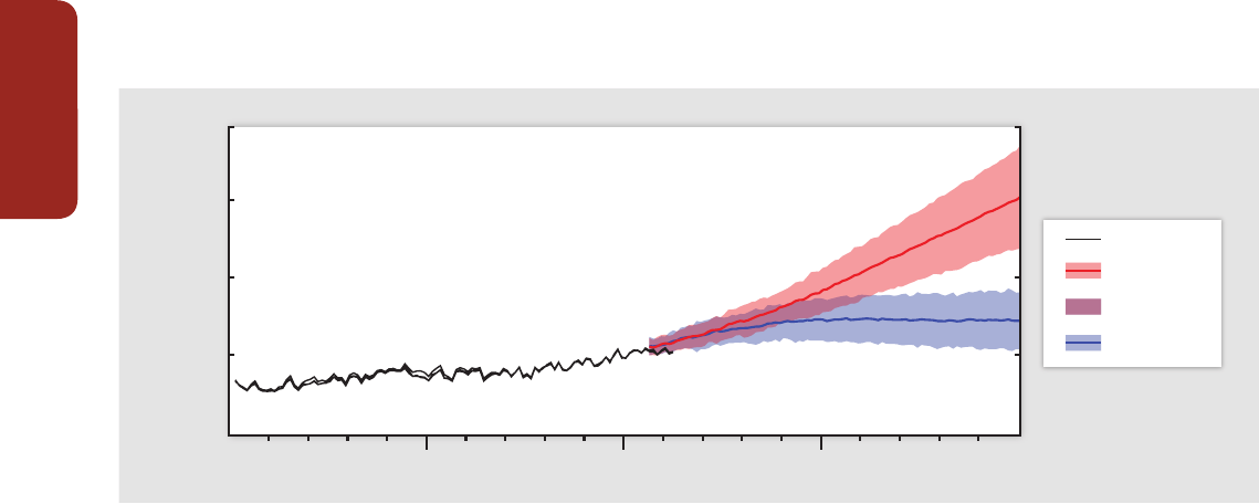
Cross-Chapter Box
Regional Climate Summary Figures
138
RC
1), including the WGI multi-model mean values; the WGI individual model values; the WGI measure of baseline (“internal”) variability; and the
WGI time periods for the reference (1986–2005), mid-21st century (2046–2065), and late-21st century (2081–2100) periods. The full description
of the selection of models, the selection of realizations, the definition of internal variability, and the interpolation to a common grid can be found
in WGI Chapter 12 and Annex I.
In contrast to the Coupled Model Intercomparison Project Phase 3 (CMIP3) (Meehl et al., 2007), which used the IPCC Special Report on Emission
Scenarios (SRES) emission scenarios (IPCC, 2000), CMIP5 uses the Representative Concentration Pathways (RCPs) (van Vuuren et al., 2011) to
characterize possible trajectories of climate forcing over the 21st century. The WGII regional climate projection maps include RCP2.6 and RCP8.5,
which represent the high and low end of the RCP range at the end of the 21st century. Projected changes in global mean temperature are
similar across the RCPs over the next few decades (Figure RC-1; WGI Figure 12.5). During this near-term era of committed climate change, risks
will evolve as socioeconomic trends interact with the changing climate. In addition, societal responses, particularly adaptations, will influence
near-term outcomes. In the second half of the 21st century and beyond, the magnitude of global temperature increase diverges across the RCPs
(Figure RC-1; WGI Figure 12.5). For this longer-term era of climate options, near-term and longer-term mitigation and adaptation, as well as
development pathways, will determine the risks of climate change. The benefits of mitigation and adaptation thereby occur over different but
overlapping time frames, and present-day choices thus affect the risks of climate change throughout the 21st century.
The projection maps plot differences in annual average temperature and precipitation between the future and reference periods (Figures RC-2
and RC-3), categorized into four classes. The classes are constructed based on the IPCC uncertainty guidance, providing a quantitative basis for
assigning likelihood (Mastrandrea et al., 2010), with likely defined as 66 to 100% and very likely defined as 90 to 100%.
Observed
RCP2.6
RCP8.5
Overlap
1900 1950 2000 2050 2100
6
4
2
0
–2
(˚C relative to
1986–2005
)
Global mean temperature change
Figure RC-1 | Observed and projected changes in global annual average temperature. Values are expressed relative to 1986–2005. Black lines show the Goddard
Institute for Space Studies Surface Temperature Analysis (GISTEMP), National Climate Data Center Merged Land–Ocean Surface Temperature (NCDC-MLOST), and
Hadley Centre/Climatic Research Unit gridded surface temperature data set 4.2 (HadCRUT4.2) estimates from observational measurements. Blue and red lines and
shading denote the ensemble mean and ±1.64 standard deviation range, based on Coupled Model Intercomparison Project Phase 5 (CMIP5) simulations from 32
models for Representative Concentration Pathway (RCP) 2.6 and 39 models for RCP8.5.
The classifications in the WGII regional climate projection figures are based on two aspects of likelihood (e.g., WGI Box 12.1 and Knutti et al.,
2010). The first is the likelihood that projected changes exceed differences arising from internal climate variability (e.g., Tebaldi et al., 2011). The
second is agreement among models on the sign of change (e.g., Christensen et al., 2007; and IPCC, 2012).
The four classifications of projected change depicted in the WGII regional climate maps are:
1) Solid colors indicate areas with very strong agreement, where the multi-model mean change is greater than twice the baseline variability
(natural internal variability in 20-year means), and greater than or equal to 90% of models agree on sign of change. These criteria (and the
areas that fall into this category) are identical to the highest confidence category in WGI Box 12.1. This category supersedes other categories
in the WGII regional climate maps.
2) Colors with white dots indicate areas with strong agreement, where 66% or more of models show change greater than the baseline
variability, and 66% or more of models agree on sign of change.
3) Gray indicates areas with divergent changes, where 66% or more of models show change greater than the baseline variability, but fewer
than 66% agree on sign of change.
4) Colors with diagonal lines indicate areas with little or no change, where fewer than 66% of models show change greater than the baseline
variability. It should be noted that areas that fall in this category for the annual average could still exhibit significant change at seasonal,
monthly, and/or daily time scales.
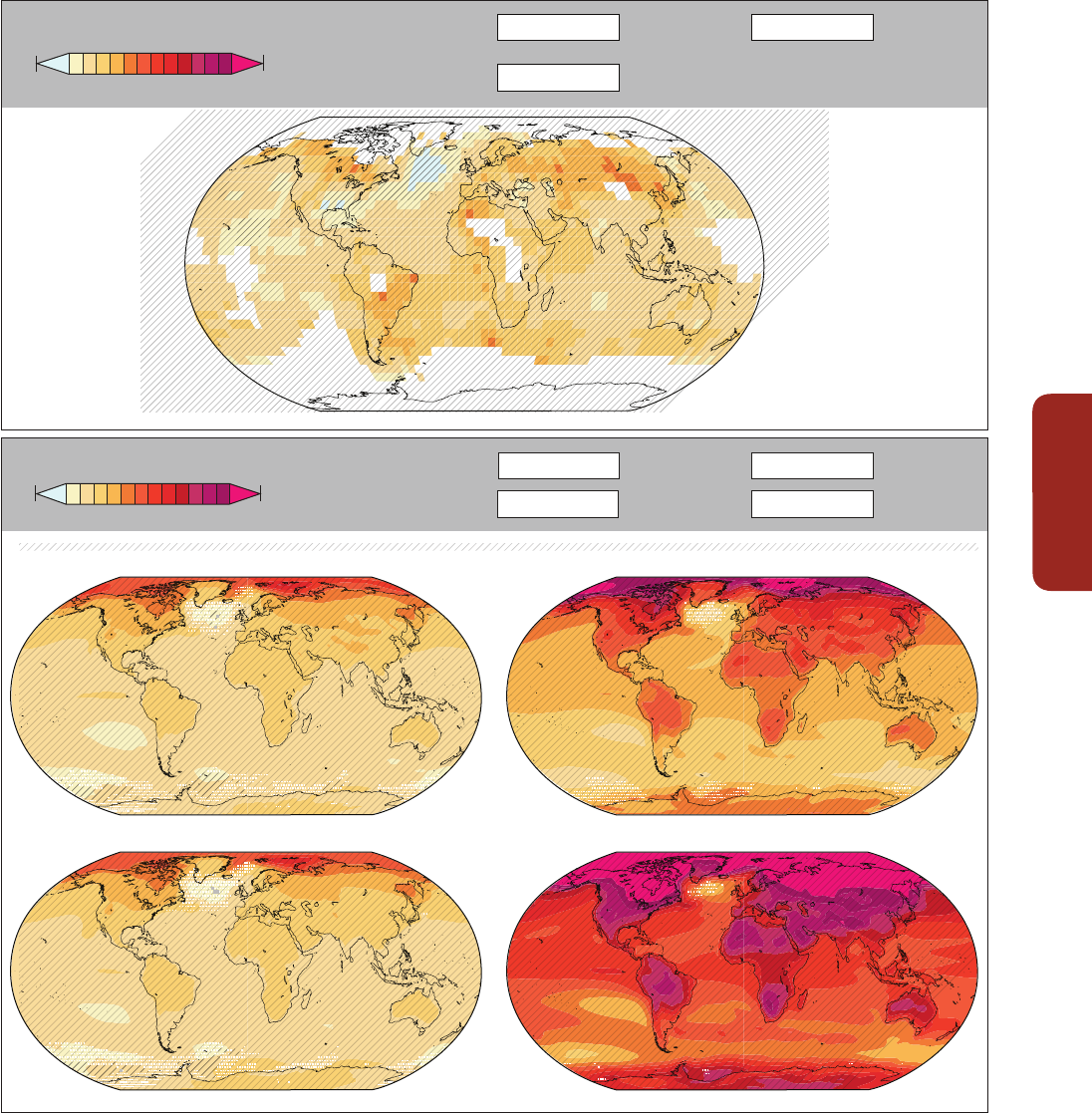
RC
Regional Climate Summary Figures
Cross-Chapter Box
139
Difference from
1986–2005 mean (
˚
C)
Projected Temperature Change
0 2 4 6
–0.5 11.7
Solid Color
Strong
agreement
Very strong
agreement
Little or
no change
Gray
Divergent
changes
Diagonal Lines
White Dots
Observed Temperature Change
Based on trend over
1901–2012 (
˚
C over period)
Diagonal Lines
Trend not
statistically
significant
White
Insufficient
data
Solid Color
Significant
trend
0 2 4 6
–0.5 11.7
RCP2.6 mid 21st century RCP8.5 mid 21st century
RCP2.6 late 21st century RCP8.5 late 21st century
Figure RC-2 |
Observed and projected changes in annual average surface temperature. (A) Map of observed annual average temperature change from 1901 to 2012, derived
from a linear trend where sufficient data permit a robust estimate (i.e., only for grid boxes with greater than 70% complete records and more than 20% data availability in the
first and last 10% of the time period); other areas are white. Solid colors indicate areas where trends are significant at the 10% level (after accounting for autocorrelation
effects on significance testing). Diagonal lines indicate areas where trends are not significant. Observed data (range of grid-point values: –0.53 to +2.50°C over period) are
from WGI AR5 Figures SPM.1 and 2.21. (B) Coupled Model Intercomparison Project Phase 5 (CMIP5) multi-model mean projections of annual average temperature changes for
2046–2065 and 2081–2100 under Representative Concentration Pathway (RCP) 2.6 and 8.5, relative to 1986–2005. Solid colors indicate areas with very strong agreement,
where the multi-model mean change is greater than twice the baseline variability (natural internal variability in 20-year means) and ≥90% of models agree on sign of change.
Colors with white dots indicate areas with strong agreement, where ≥66% of models show change greater than the baseline variability and ≥66% of models agree on sign of
change. Gray indicates areas with divergent changes, where ≥66% of models show change greater than the baseline variability, but <66% agree on sign of change. Colors
with diagonal lines indicate areas with little or no change, where <66% of models show change greater than the baseline variability, although there may be significant change
at shorter timescales such as seasons, months, or days. Analysis uses model data from WGI AR5 Figure SPM.8, Box 12.1, and Annex I. The range of grid-point values for the
multi-model mean is: +0.19 to +4.08˚C for mid 21st century of RCP2.6; +0.06 to +3.85˚C for late 21st century of RCP2.6; +0.70 to +7.04˚C for mid 21st century of RCP8.5;
and +1.38 to +11.71°C for late 21st century of RCP8.5.
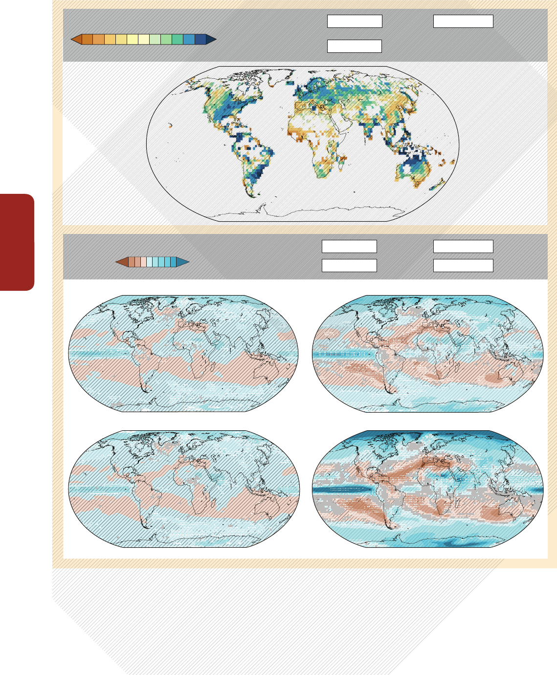
Cross-Chapter Box
Regional Climate Summary Figures
140
RC
Projected Precipitation Change
RCP2.6 mid 21st century RCP8.5 mid 21st century
RCP2.6 late 21st century RCP8.5 late 21st century
–20 0 20 40
Observed Precipitation Change
–
5 0 5 25102.5
–
2.5 50
–
10
–
50
–
25
–
100
Diagonal Lines
Trend not
statistically
significant
White
Insufficient
data
Solid Color
Significant
trend
Solid Color
Strong
agreement
Very strong
agreement
Little or
no change
Gray
Divergent
changes
Diagonal Lines
White Dots
Difference from
1986–2005 mean (%)
Trend in annual
precipitation
over 1951–2010
(mm/year per decade)
Figure RC-3 | Observed and projected changes in annual average precipitation. (A) Map of observed annual precipitation change from 1951–2010, derived from a linear trend
where sufficient data permit a robust estimate (i.e., only for grid boxes with greater than 70% complete records and more than 20% data availability in the first and last 10% of
the time period); other areas are white. Solid colors indicate areas where trends are significant at the 10% level (after accounting for autocorrelation effects on significance
testing). Diagonal lines indicate areas where trends are not significant. Observed data (range of grid-point values: –185 to +111 mm/year per decade) are fr
om WGI AR5 Figures
SPM.2 and 2.29. (B) Coupled Model Intercomparison Project Phase 5 (CMIP5) multi-model average percent changes in annual mean precipitation for 2046–2065 and
2081–2100 under Representative Concentration Pathway (RCP) 2.6 and 8.5, relative to 1986–2005. Solid colors indicate areas with very strong agreement, where the
multi-model mean change is greater than twice the baseline variability (natural internal variability in 20-yr means) and ≥90% of models agree on sign of change. Colors with
white dots indicate areas with strong agreement, where ≥66% of models show change greater than the baseline variability and ≥66% of models agree on sign of change. Gray
indicates areas with divergent changes, where ≥66% of models show change greater than the baseline variability, but <66% agree on sign of change. Colors with diagonal lines
indicate areas with little or no change, where <66% of models show change greater than the baseline variability, although there may be significant change at shorter timescales
such as seasons, months, or days. Analysis uses model data from WGI AR5 Figure SPM.8, Box 12.1, and Annex I. The range of grid-point values for the multi-model mean is: –10
to +24% for mid 21st century of RCP2.6; –9 to +22% for late 21st century of RCP2.6; –19 to +57% for mid 21st century of RCP8.5; and –34 to +112% for late 21st century
of RCP8.5.

RC
Regional Climate Summary Figures
Cross-Chapter Box
141
Christensen, J.H., B. Hewitson, A. Busuioc, A. Chen, X. Gao, I. Held, R. Jones, R.K. Kolli, W.-T. Kwon, R. Laprise, V. Magaña Rueda, L. Mearns, C.G. Menéndez, J. Räisänen, A.
Rinke, A. Sarr, and P. Whetton, 2007: Regional climate projections. Climate Change 2007: The Physical Science Basis. Contribution of Working Group I to the Fourth
Assessment Report of the Intergovernmental Panel on Climate Change [Solomon, S., D. Qin, M. Manning, Z. Chen, M. Marquis, K.B. Averyt, M. Tignor, and H.L. Miller
(eds.)]. Cambridge University Press, Cambridge, UK and New York, NY, USA, pp. 847-940.
IPCC, 2000: Special Report on Emissions Scenarios [Nakicenovic, N. and R. Swart (eds.)]. Cambridge University Press, Cambridge, UK, 570 pp.
IPCC, 2012: Managing the Risks of Extreme Events and Disasters to Advance Climate Change Adaptation. A Special Report of Working Groups I and II of the
Intergovernmental Panel on Climate Change [Field, C.B., V. Barros, T.F. Stocker, D. Qin, D.J. Dokken, K.L. Ebi, M.D. Mastrandrea, K.J. Mach, G.-K. Plattner, S.K. Allen, M.
Tignor, and P.M. Midgley (eds.)]. Cambridge University Press, Cambridge, UK and New York, NY, USA, 582 pp.
Knutti, R., R. Furrer, C. Tebaldi, J. Cermak, and G.A. Meehl, 2010: Challenges in combining projections from multiple climate models. Journal of Climate, 23(10), 2739-2758.
Mastrandrea, M.D., C.B. Field, T.F. Stocker, O. Edenhofer, K.L. Ebi, D.J. Frame, H. Held, E. Kriegler, K.J. Mach, P.R. Matschoss, G.-K. Plattner, G.W. Yohe, and F.W. Zwiers, 2010:
Guidance Note for Lead Authors of the IPCC Fifth Assessment Report on Consistent Treatment of Uncertainties. Intergovernmental Panel on Climate Change (IPCC),
www.ipcc.ch/pdf/supporting-material/uncertainty-guidance-note.pdf.
Meehl, G.A., C. Covey, K.E. Taylor, T. Delworth, R.J. Stouffer, M. Latif, B. McAvaney, and J.F.B. Mitchell, 2007: The WCRP CMIP3 multimodel dataset – a new era in climate
change research. Bulletin of the American Meteorological Society, 88(9), 1383-1394.
Taylor, K.E., R.J. Stouffer, and G.A. Meehl, 2012: An overview of CMIP5 and the experiment design. Bulletin of the American Meteorological Society, 93(4), 485-498.
Tebaldi, C., J.M. Arblaster, and Reto Knutti, 2011: Mapping model agreement on future climate projections. Geophysical Research Letters, 38(23), L23701,
doi:10.1029/2011GL049863.
van Vuuren, D.P., J. Edmonds, M. Kainuma, K. Riahi, A. Thomson, K. Hibbard, G.C. Hurtt, T. Kram, V. Krey, J.-F. Lamarque, T. Masui, M. Meinshausen, N. Nakicenovic, S.J.
Smith, and S.K. Rose 2011: The representative concentration pathways: an overview. Climatic Change, 109(1-2), 5-31.
References
Diffenbaugh, N.S., D.A. Stone, P. Thorne, F. Giorgi, B.C. Hewitson, R.G. Jones, and G.J. van Oldenborgh, 2014: Cross-chapter box on the regional climate summary
figures. In: Climate Change 2014: Impacts, Adaptation, and Vulnerability. Part A: Global and Sectoral Aspects. Contribution of Working Group II to the
Fifth Assessment Report of the Intergovernmental Panel on Climate Change [Field, C.B., V.R. Barros, D.J. Dokken, K.J. Mach, M.D. Mastrandrea, T.E. Bilir, M.
Chatterjee, K.L. Ebi, Y.O. Estrada, R.C. Genova, B. Girma, E.S. Kissel, A.N. Levy, S. MacCracken, P.R. Mastrandrea, and L.L. White (eds.)]. Cambridge University
Press, Cambridge, United Kingdom and New York, NY, USA, pp. 137-141.
This cross-chapter box should be cited as:

Impact of Climate Change on
Freshwater Ecosystems due to
Altered River Flow Regimes
Petra Döll (Germany), Stuart E. Bunn (Australia)
RF
143
It is widely acknowledged that the flow regime is a primary determinant of the structure and
function of rivers and their associated floodplain wetlands, and flow alteration is considered to be
a serious and continuing threat to freshwater ecosystems (Bunn and Arthington, 2002; Poff and
Zimmerman, 2010; Poff et al., 2010). Most species distribution models do not consider the effect
of changing flow regimes (i.e., changes to the frequency, magnitude, duration, and/or timing of
key flow parameters) or they use precipitation as proxy for river flow (Heino et al., 2009).
There is growing evidence that climate change will significantly alter ecologically important
attributes of hydrologic regimes in rivers and wetlands, and exacerbate impacts from human
water use in developed river basins (medium confidence; Xenopoulos et al., 2005; Aldous et al.,
2011). By the 2050s, climate change is projected to impact river flow characteristics such as
long-term average discharge, seasonality, and statistical high flows (but not statistical low flows)
more strongly than dam construction and water withdrawals have done up to around the year
2000 (Figure RF-1; Döll and Zhang, 2010). For one climate scenario (Special Report on Emission
Scenarios (SRES) A2 emissions, Met Office Hadley Centre climate prediction model 3 (HadCM3)),
15% of the global land area may be negatively affected, by the 2050s, by a decrease of fish
species in the upstream basin of more than 10%, as compared to only 10% of the land area that
has already suffered from such decreases due to water withdrawals and dams (Döll and Zhang,
2010). Climate change may exacerbate the negative impacts of dams for freshwater ecosystems
but may also provide opportunities for operating dams and power stations to the benefit of
riverine ecosystems. This is the case if total runoff increases and, as occurs in Sweden, the annual
hydrograph becomes more similar to variation in electricity demand, that is, with a lower spring
flood and increased runoff during winter months (Renofalt et al., 2010).
Because biota are often adapted to a certain level of river flow variability, the projected larger
variability of river flows that is due to increased climate variability is likely to select for generalist
or invasive species (Ficke et al., 2007). The relatively stable habitats of groundwater-fed streams in
snow-dominated or glacierized basins may be altered by reduced recharge by meltwater and as a
result experience more variable (possibly intermittent) flows (Hannah et al., 2007). A high-impact
change of flow variability is a flow regime shift from intermittent to perennial or vice versa. It is
projected that until the 2050s, river flow regime shifts may occur on 5 to 7% of the global land
area, mainly in semiarid areas (Döll and Müller Schmied, 2012; see Table 3-2 in Chapter 3).
In Africa, one third of fish species and one fifth of the endemic fish species occur in eco-regions
that may experience a change in discharge or runoff of more than 40% by the 2050s (Thieme et
al., 2010). Eco-regions containing more than 80% of Africa’s freshwater fish species and several
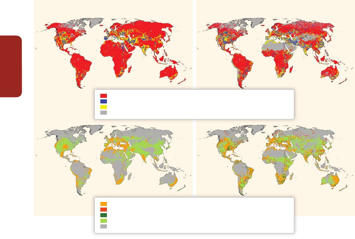
Cross-Chapter Box
Impact of Climate Change on Freshwater Ecosystems due to Altered River Flow Regimes
144
RF
outstanding ecological and evolutionary phenomena are likely to experience hydrologic conditions substantially different from the present,
with alterations in long-term average annual river discharge or runoff of more than 10% due to climate change and water use (Thieme et al.,
2010).
As a result of increased winter temperatures, freshwater ecosystems in basins with significant snow storage are affected by higher river
flows in winter, earlier spring peak flows, and possibly reduced summer low flows (Section 3.2.3). Strongly increased winter peak flows may
lead to a decline in salmonid populations in the Pacific Northwest of the USA of 20 to 40% by the 2050s (depending on the climate model)
due to scouring of the streambed during egg incubation, the relatively pristine high-elevation areas being affected most (Battin et al., 2007).
Reductions in summer low flows will increase the competition for water between ecosystems and irrigation water users (Stewart et al.,
2005). Ensuring environmental flows through purchasing or leasing water rights and altering reservoir release patterns will be an important
adaptation strategy (Palmer et al., 2009).
Mean annual river flow Low flow Q
90
Monthly river flow exceeded in 9 out of 10 months
Impact of climate change at least twice as strong as impact of water withdrawals and dams on natural flow
Impact of water withdrawals and dams on natural flow at least twice as strong as impact of climate change
None of the two impacts is more than twice as strong as the other
Information not computable
Climate change exacerbates past impacts of water withdrawals and dams on natural flow that reduced flow
Climate change exacerbates past impacts of water withdrawals and dams on natural flow that increased flow
Climate change mitigates past impacts of water withdrawals and dams on natural flow that reduced flow
Climate change mitigates past impacts of water withdrawals and dams on natural flow that increased flow
Past impacts < 1% or information not computable
Figure RF-1 |
Impact of climate change relative to the impact of water withdrawals and dams on natural flows for two ecologically relevant river flow characteristics (mean annual river
flow and monthly low flow Q
90
), computed by a global water model (Döll and Zhang, 2010). Impact of climate change is the percent change of flow between 1961–1990 and 2041–2070
according to the emissions scenario A2 as implemented by the global climate model Met Office Hadley Centre Coupled Model, version 3 (HadCM3). Impact of water withdrawals and
reservoirs is computed by running the model with and without water withdrawals and dams that existed in 2002. Please note that the figure does not reflect spatial differences in the
magnitude of change.
Observations and models suggest that global warming impacts on glacier and snow-fed streams and rivers will pass through two contrasting
phases (Burkett et al., 2005; Vuille et al., 2008; Jacobsen et al., 2012). In the first phase, when river discharge is increased as a result of
intensified melting, the overall diversity and abundance of species may increase. However, changes in water temperature and stream flow may
have negative impacts on narrow range endemics (Jacobsen et al., 2012). In the second phase, when snowfields melt early and glaciers have
shrunken to the point that late-summer stream flow is reduced, broad negative impacts are foreseen, with species diversity rapidly declining
once a critical threshold of roughly 50% glacial cover is crossed (Figure RF-2).
River discharge also influences the response of river temperatures to increases of air temperature. Globally averaged, air temperature increases
of 2°C, 4°C, and 6°C are estimated to lead to increases of annual mean river temperatures of 1.3°C, 2.6°C, and 3.8°C, respectively (van Vliet
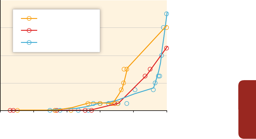
RF
Impact of Climate Change on Freshwater Ecosystems due to Altered River Flow Regimes
Cross-Chapter Box
145
Aldous, A., J. Fitzsimons, B. Richter, and L. Bach, 2011: Droughts, floods and freshwater ecosystems: evaluating climate change impacts and developing adaptation
strategies. Marine and Freshwater Research, 62(3), 223-231.
Battin, J., M.W. Wiley, M.H. Ruckelshaus, R.N. Palmer, E. Korb, K.K. Bartz, and H. Imaki, 2007: Projected impacts of climate change on salmon habitat restoration.
Proceedings of the National Academy of Sciences of the United States of America, 104(16), 6720-6725.
Bunn, S.E. and A.H. Arthington, 2002: Basic principles and ecological consequences of altered flow regimes for aquatic biodiversity. Environmental Management, 30(4),
492-507.
Burkett, V., D. Wilcox, R. Stottlemyer, W. Barrow, D. Fagre, J. Baron, J. Price, J. Nielsen, C. Allen, D. Peterson, G. Ruggerone, and T. Doyle, 2005: Nonlinear dynamics in
ecosystem response to climatic change: case studies and policy implications. Ecological Complexity, 2(4), 357-394.
Döll, P. and H. Müller Schmied, 2012: How is the impact of climate change on river flow regimes related to the impact on mean annual runoff? A global-scale analysis.
Environmental Research Letters, 7(1), 014037, doi:10.1088/1748-9326/7/1/014037.
Döll, P. and J. Zhang, 2010: Impact of climate change on freshwater ecosystems: a global-scale analysis of ecologically relevant river flow alterations. Hydrology and Earth
System Sciences, 14(5), 783-799.
Ficke, A.D., C.A. Myrick, and L.J. Hansen, 2007: Potential impacts of global climate change on freshwater fisheries. Reviews in Fish Biology and Fisheries, 17(4), 581-613.
Hannah, D.M., L.E. Brown, A.M. Milner, A.M. Gurnell, G.R. McGregord, G.E. Petts, B.P.G. Smith, and D.L. Snook, 2007: Integrating climate-hydrology-ecology for alpine river
systems. Aquatic Conservation: Marine and Freshwater Ecosystems, 17(6), 636-656.
Heino, J., R. Virkalla, and H. Toivonen, 2009: Climate change and freshwater biodiversity: detected patterns, future trends and adaptations in northern regions. Biological
Reviews, 84(1), 39-54.
Jacobsen, D., A.M. Milner, L.E. Brown, and O. Dangles, 2012: Biodiversity under threat in glacier-fed river systems. Nature Climate Change, 2(5), 361-364.
Palmer, M.A., D.P. Lettenmaier, N.L. Poff, S.L. Postel, B. Richter, and R. Warner, 2009: Climate change and river ecosystems: protection and adaptation options.
Environmental Management, 44(6), 1053-1068.
Poff, N.L. and J.K.H. Zimmerman, 2010: Ecological responses to altered flow regimes: a literature review to inform the science and management of environmental flows.
Freshwater Biology, 55(1), 194-205.
Poff, N.L., B.D. Richter, A.H. Arthington, S.E. Bunn, R.J. Naiman, E. Kendy, M. Acreman, C. Apse, B.P. Bledsoe, M.C. Freeman, J. Henriksen, R.B. Jacobson, J.G. Kennen, D.M.
Merritt, J.H. O’Keeffe, J.D. Olden, K. Rogers, R.E. Tharme, and A. Warner, 2010: The ecological limits of hydrologic alteration (ELOHA): a new framework for developing
regional environmental flow standards. Freshwater Biology, 55(1), 147-170.
References
Glacier cover in catchment (%)
Accumulated regional species loss
100 80 60 40 20 0
0
4
8
12
16
European Alps
Alaskan Coastal Range
Ecuadorian Andes
Figure RF-2 |
Accumulated loss of regional species richness (gamma diversity) of macroinvertebrates as a function of glacial cover in catchment. Obligate glacial river
macroinvertebrates begin to disappear from assemblages when glacial cover in the catchment drops below approximately 50%, and 9 to 14 species are predicted to be lost with
the complete disappearance of glaciers in each region, corresponding to 11, 16, and 38% of the total species richness in the three study regions in Ecuador, Europe, and Alaska.
Data are derived from multiple river sites from the Ecuadorian Andes and Swiss and Italian Alps, and a temporal study of a river in the Coastal Range Mountains of southeast
Alaska over nearly three decades of glacial shrinkage. Each data point represents a river site (Europe or Ecuador) or date (Alaska), and lines are Lowess fits. (Adapted by
permission from Jacobsen et al., 2012.)
et al., 2011). Discharge decreases of 20% and 40% are computed to result in additional increases of river water temperature of 0.3° C and
0.8°C on average (van Vliet et al., 2011). Therefore, where rivers will experience drought more frequently in the future, freshwater-dependent
biota will suffer not only directly by changed flow conditions but also by drought-induced river temperature increases, as well as by related
decreased oxygen and increased pollutant concentrations.

Cross-Chapter Box
Impact of Climate Change on Freshwater Ecosystems due to Altered River Flow Regimes
146
RF
Döll, P. and S.E. Bunn, 2014: Cross-chapter box on the impact of climate change on freshwater ecosystems due to altered river flow regimes. In: Climate Change
2014: Impacts, Adaptation, and Vulnerability. Part A: Global and Sectoral Aspects. Contribution of Working Group II to the Fifth Assessment Report of the
Intergovernmental Panel on Climate Change [Field, C.B., V.R. Barros, D.J. Dokken, K.J. Mach, M.D. Mastrandrea, T.E. Bilir, M. Chatterjee, K.L. Ebi, Y.O. Estrada,
R.C. Genova, B. Girma, E.S. Kissel, A.N. Levy, S. MacCracken, P.R. Mastrandrea, and L.L. White (eds.)]. Cambridge University Press, Cambridge, United King-
dom and New York, NY, USA, pp. 143-146.
This cross-chapter box should be cited as:
Renofalt, B.M., R. Jansson, and C. Nilsson, 2010: Effects of hydropower generation and opportunities for environmental flow management in Swedish riverine
ecosystems. Freshwater Biology, 55(1), 49-67.
Stewart, I., D. Cayan, and M. Dettinger, 2005: Changes toward earlier streamflow timing across western North America. Journal of Climate, 18(8), 1136-1155.
Thieme, M.L., B. Lehner, R. Abell, and J. Matthews, 2010: Exposure of Africa’s freshwater biodiversity to a changing climate. Conservation Letters, 3(5), 324-331.
van Vliet, M.T.H., F. Ludwig, J.J.G. Zwolsman, G.P. Weedon, and P. Kabat, 2011: Global river temperatures and sensitivity to atmospheric warming and changes in river
flow. Water Resources Research, 47(2), W02544, doi:10.1029/2010WR009198.
Vuille, M., B. Francou, P. Wagnon, I. Juen, G. Kaser, B.G. Mark, and R.S. Bradley, 2008: Climate change and tropical Andean glaciers: past, present and future. Earth-Science
Reviews, 89(3-4), 79-96.
Xenopoulos, M., D. Lodge, J. Alcamo, M. Marker, K. Schulze, and D. Van Vuuren, 2005: Scenarios of freshwater fish extinctions from climate change and water withdrawal.
Global Change Biology, 11(10), 1557-1564.

Building Long-Term
Resilience from Tropical
Cyclone Disasters
Yoshiki Saito (Japan), Kathleen McInnes (Australia)
TC
147
Tropical cyclones (also referred to as hurricanes and typhoons in some regions) cause powerful
winds, torrential rains, high waves, and storm surge, all of which can have major impacts on
society and ecosystems. Bangladesh and India suffer 86% of mortality from tropical cyclones
(Murray et al., 2012), which occurs mainly during the rarest and most severe storm categories (i.e.,
Categories 3, 4, and 5 on the Saffir–Simpson scale).
About 90 tropical cyclones occur globally each year (Seneviratne et al., 2012) although interannual
variability is large. Changes in observing techniques, particularly after the introduction of satellites
in the late 1970s, confounds the assessment of trends in tropical cyclone frequencies and
intensities, which leads to low confidence that any observed long-term (i.e., 40 years or more)
increases in tropical cyclone activity are robust, after accounting for past changes in observing
capability (Seneviratne et al., 2012; Chapter 2). There is also low confidence in the detection and
attribution of century scale trends in tropical cyclones. Future changes to tropical cyclones arising
from climate change are likely to vary by region. This is because there is medium confidence
that for certain regions, shorter-term forcing by natural and anthropogenic aerosols has had a
measurable effect on tropical cyclones. Tropical cyclone frequency is likely to decrease or remain
unchanged over the 21st century, while intensity (i.e., maximum wind speed and rainfall rates) is
likely to increase (WGI AR5 Section 14.6). Regionally specific projections have lower confidence
(see WGI AR5 Box 14.2).
Longer-term impacts from tropical cyclones include salinization of coastal soils and water supplies
and subsequent food and water security issues from the associated storm surge and waves (Terry
and Chui, 2012). However, preparation for extreme tropical cyclone events through improved
governance and development to reduce their impacts provides an avenue for building resilience to
longer-term changes associated with climate change.
Asian deltas are particularly vulnerable to tropical cyclones owing to their large population density
in expanding urban areas (Nicholls et al., 2007). Extreme cyclones in Asia since 1970 caused more
than 0.5 million fatalities (Murray et al., 2012), for example, cyclones Bhola in 1970, Gorky in
1991, Thelma in 1998, Gujarat in 1998, Orissa in 1999, Sidr in 2007, and Nargis in 2008. Tropical
cyclone Nargis hit Myanmar on May 2, 2008 and caused more than 138,000 fatalities. Several-
meter high storm surges widely flooded densely populated coastal areas of the Irrawaddy Delta
and surrounding areas (Revenga et al., 2003; Brakenridge et al., 2013). The flooded areas were
captured by a NASA Moderate Resolution Imaging Spectrometer (MODIS) image on May 5, 2008
(see Figure TC-1).
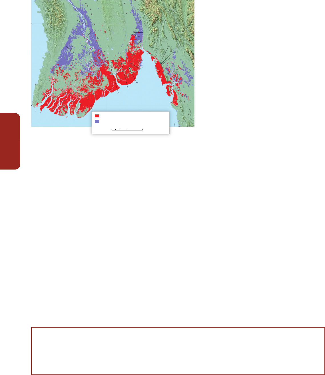
Cross-Chapter Box
Building Long-Term Resilience from Tropical Cyclone Disasters
148
TC
Murray et al. (2012) compared the response to cyclone
Sidr in Bangladesh in 2007 and Nargis in Myanmar in
2008 and demonstrated how disaster risk reduction
methods could be successfully applied to climate change
adaptation. Sidr, despite being of similar strength to
Nargis, caused far fewer fatalities (3400 compared to more
than 138,000) and this was attributed to advancement
in preparedness and response in Bangladesh through
experience in previous cyclones such as Bhola and Gorky.
The responses included the construction of multistoried
cyclone shelters, improvement of forecasting and warning
capacity, establishing a coastal volunteer network,
and coastal reforestation of mangroves. Disaster risk
management strategies for tropical cyclones in coastal
areas create protective measures, anticipate and plan for
extreme events, and increase the resilience of potentially
exposed communities. The integration of activities relating
to education, training, and awareness-raising into relevant
ongoing processes and practices is important for the long-
term success of disaster risk reduction and management
(Murray et al., 2012). However, Birkmann and Teichman
(2010) caution that while the combination of risk reduction
and climate change adaptation strategies may be desirable,
different spatial and temporal scales, norm systems, and
knowledge types and sources between the two goals can
confound their effective combination.
Birkman, J. and K. von Teichman, 2010: Integrating disaster risk reduction and climate change adaptation: key challenges – scales, knowledge and norms. Sustainability
Science, 5, 171-184.
Brakenridge, G.R., J.P.M. Syvitski, I. Overeem, S.A. Higgins, A.J. Kettner, J.A. Stewart-Moore, and R. Westerhoff, 2013: Global mapping of storm surges and the assessment
of delta vulnerability. Natural Hazards, 66, 1295-1312, doi:10.1007/s11069-012-0317-z.
Murray V., G. McBean, M. Bhatt, S. Borsch, T.S. Cheong, W.F. Erian, S. Llosa, F. Nadim, M. Nunez, R. Oyun, and A.G. Suarez, 2012: Case studies. In: Managing the Risks
of Extreme Events and Disasters to Advance Climate Change Adaptation. A Special Report of Working Groups I and II of the Intergovernmental Panel on Climate
Change [Field, C.B., V. Barros, T.F. Stocker, D. Qin, D.J. Dokken, K.L. Ebi, M.D. Mastrandrea, K.J. Mach, G.-K. Plattner, S.K. Allen, M. Tignor, and P.M. Midgley (eds.)].
Cambridge University Press, Cambridge, UK and New York, NY, USA, pp. 487-542.
Nicholls, R.J., 2007: Adaptation Options for Coastal Areas and Infrastructure: An Analysis for 2030. Report to the United Nations Framework Convention on Climate
Change (UNFCCC), UNFCCC Secretariat, Bonn, Germany, 35 pp.
Revenga, C., J. Nackoney, E. Hoshino, Y. Kura, and J. Maidens, 2003: Watersheds of Asia and Oceania: AS 12 Irrawaddy. In: Water Resources eAtlas: Watersheds of the
World. A collaborative product of the International Union for Conservation of Nature (IUCN), the International Water Management Institute (IWMI), the Ramsar
Convention Bureau, and the World Resources Institute (WRI), WRI, Washington, DC, USA, pdf.wri.org/watersheds_2003/as13.pdf.
Seneviratne, S.I., N. Nicholls, D. Easterling, C.M. Goodess, S. Kanae, J. Kossin, Y. Luo, J. Marengo, K. McInnes, M. Rahimi, M. Reichstein, A. Sorteberg, C. Vera, and X. Zhang,
2012: Changes in climate extremes and their impacts on the natural physical environment. In: Managing the Risks of Extreme Events and Disasters to Advance
Climate Change Adaptation. A Special Report of Working Groups I and II of the Intergovernmental Panel on Climate Change [Field, C.B., V. Barros, T.F. Stocker, D. Qin,
D.J. Dokken, K.L. Ebi, M.D. Mastrandrea, K.J. Mach, G.-K. Plattner, S.K. Allen, M. Tignor, and P.M. Midgley (eds.)]. Cambridge University Press, Cambridge, UK and New
York, NY, USA, pp. 109-230.
Terry, J. and T.F.M. Chui, 2012: Evaluating the fate of freshwater lenses on atoll islands after eustatic sea level rise and cyclone driven inundation: a modelling approach.
Global and Planetary Change, 88-89, 76-84.
Saito, Y. and K.L. McInnes, 2014: Cross-chapter box on building long-term resilience from tropical cyclone disasters. In: Climate Change 2014: Impacts,
Adaptation, and Vulnerability. Part A: Global and Sectoral Aspects. Contribution of Working Group II to the Fifth Assessment Report of the
Intergovernmental Panel on Climate Change [Field, C.B., V.R. Barros, D.J. Dokken, K.J. Mach, M.D. Mastrandrea, T.E. Bilir, M. Chatterjee, K.L. Ebi, Y.O. Estrada,
R.C. Genova, B. Girma, E.S. Kissel, A.N. Levy, S. MacCracken, P.R. Mastrandrea, and L.L. White (eds.)]. Cambridge University Press, Cambridge, United
Kingdom and New York, NY, USA, pp. 147-148.
References
Kyangin
Monyo
Minhla
Gyobingauk
Zigon
Nattalin
Paungde
Henzada
Ngathainggyaung
Yegyi
Kyonpyaw
Kangyidaung
Dassein
Kyaunggon
Wakema
Bogale
Pyapon
Kyaiklat
Ma-ubin
Yandoon
Danubyu
Taikkyi
Thonze
Tharrawaddy
Syriam
Rangoon
Mingaladon
Pyuzu
Kayan
Thetkala
Onhne
Satthwadaw
Intagwa
Thanatpin
Kamase
Pegu
Hmawbi
Hlegu
Pyinyegyi
Pyuntaza
Dai-k
Dabeinzu
Poungdawthi
Payagyi
Thaiktugon
Nyaungkashe
Pyu
Kanna banlaung
Kyaukkyi
Papun
Kyaikto
Kyaikpi
Naunggala
Naungbo
Kathapa-anauk
Thaton
Mutkyi
Khindan
Moulmein
Wagaru
Kale
Kada
0 40 80 km
Tropical cyclone Nargis storm surge in 2008
Flooded areas in previous years
18ºN
16ºN
Figure TC-1 | The intersection of inland and storm surge flooding. Red shows May 5, 2008
Moderate Resolution Imaging Spectrometer (MODIS) mapping of the tropical cyclone Nargis storm
surge along the Irrawaddy Delta and to the east, Myanmar. The purple areas to the north were
flooded by the river in prior years. (Source: Brakenridge et al., 2013.)
This cross-chapter box should be cited as:

Uncertain Trends in Major
Upwelling Ecosystems
Salvador E. Lluch-Cota (Mexico), Ove Hoegh-Guldberg (Australia), David Karl (USA), Hans O.
Pörtner (Germany), Svein Sundby (Norway), Jean-Pierre Gattuso (France)
UP
149
Upwelling is the vertical transport of cold, dense, nutrient-rich, relatively low-pH and often
oxygen-poor waters to the euphotic zone where light is abundant. These conditions trigger high
levels of primary production and a high biomass of benthic and pelagic organisms. The driving
forces of upwelling include wind stress and the interaction of ocean currents with bottom
topography. Upwelling intensity also depends on water column stratification. The major upwelling
systems of the planet, the Equatorial Upwelling System (EUS; Section 30.5.2, Figure 30.1A) and
the Eastern Boundary Upwelling Ecosystems (EBUE; Section 30.5.5, Figure 30.1A), represent only
10% of the ocean surface but contribute nearly 25% to global fish production (Figure 30.1B, Table
SM30.1).
Marine ecosystems associated with upwelling systems can be influenced by a range of “bottom-
up” trophic mechanisms, with upwelling, transport, and chlorophyll concentrations showing
strong seasonal and interannual couplings and variability. These, in turn, influence trophic transfer
up the food chain, affecting zooplankton, foraging fish, seabirds, and marine mammals.
There is considerable speculation as to how upwelling systems might change in a warming and
acidifying ocean. Globally, the heat gain of the surface ocean has increased stratification by
4% (WGI Sections 3.2, 3.3, 3.8), which means that more wind energy is needed to bring deep
waters to the surface. It is as yet unclear to what extent wind stress can offset the increased
stratification, owing to the uncertainty in wind speed trends (WGI Section 3.4.4). In the tropics,
observations of reductions in trade winds over several decades contrast more recent evidence
indicating their strengthening since the late 1990s (WGI Section 3.4.4). Observations and
modeling efforts in fact show diverging trends in coastal upwelling at the eastern boundaries
of the Pacific and the Atlantic. Bakun (1990) proposed that the difference in rates of heat gain
between land and ocean causes an increase in the pressure gradient, which results in increased
alongshore winds and leads to intensified offshore transport of surface water through Ekman
pumping and the upwelling of nutrient-rich, cold waters (Figure CC-UP). Some regional records
support this hypothesis; others do not. There is considerable variability in warming and cooling
trends over the past decades both within and among systems, making it difficult to predict
changes in the intensity of all Eastern EBUEs (Section 30.5.5).
Understanding whether upwelling and climate change will impact resident biota in an additive,
synergistic, or antagonistic manner is important for projections of how ecological goods and
services provided for human society will change. Even though upwellings may prove more
resilient to climate change than other ocean ecosystems because of their ability to function
under extremely variable conditions (Capone and Hutchins, 2013), consequences of their shifts
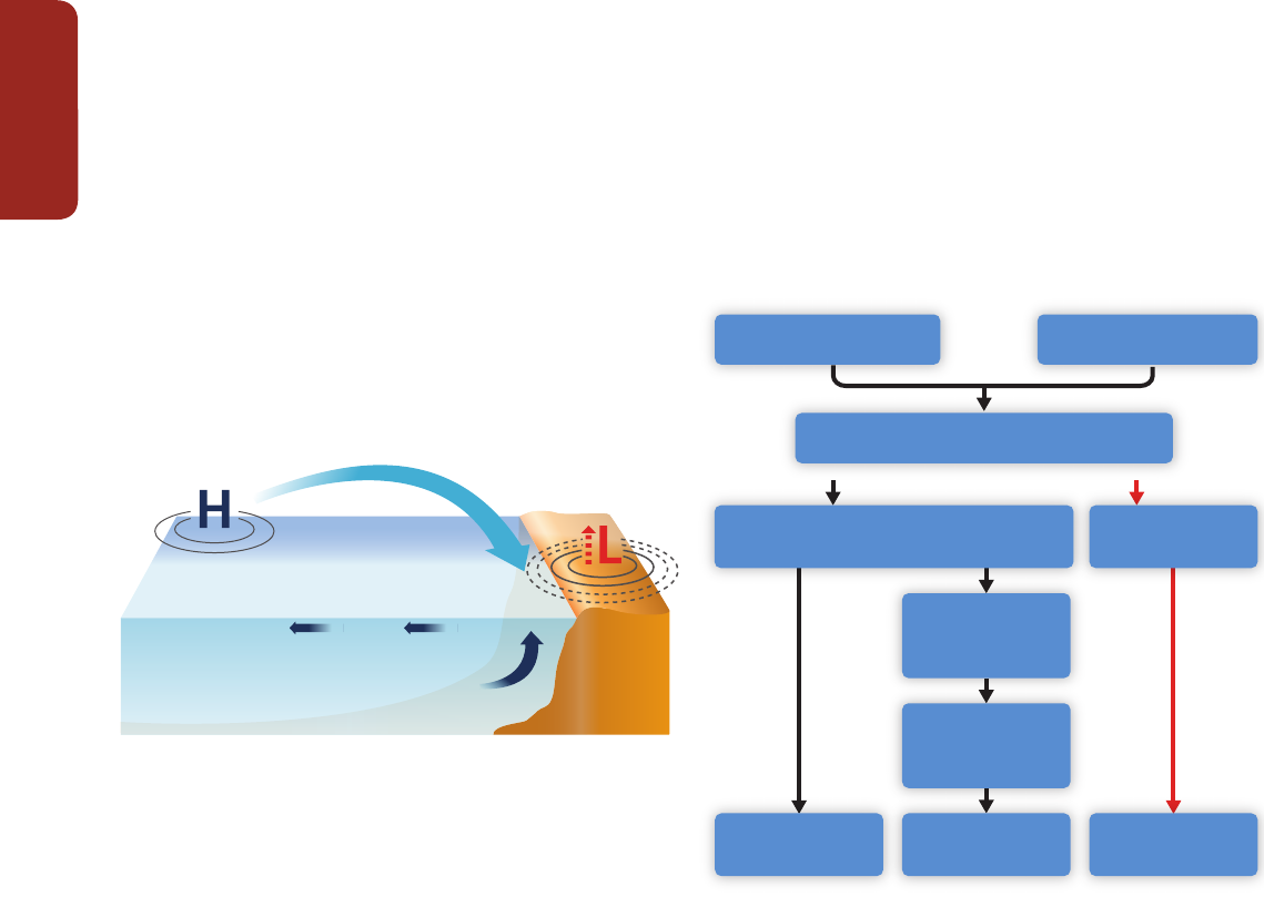
Cross-Chapter Box
Uncertain Trends in Major Upwelling Ecosystems
150
UP
are highly relevant because these systems provide a significant portion of global primary productivity and fishery catch (Figure 30.1 A, B;
Table SM30.1). Increased upwelling would enhance fisheries yields. However, the export of organic material from surface to deeper layers of
the ocean may increase and stimulate its decomposition by microbial activity, thereby enhancing oxygen depletion and CO
2
enrichment in
deeper water layers. Once this water returns to the surface through upwelling, benthic and pelagic coastal communities will be exposed to
acidified and deoxygenated water which may combine with anthropogenic impact to negatively affect marine biota and ecosystem structure
of the upper ocean (high confidence; Sections 6.3.2, 6.3.3, 30.3.2.2, 30.3.2.3). Extreme hypoxia may result in abnormal mortalities of fishes
and invertebrates (Keller et al., 2010), reduce fisheries’ catch potential, and impact aquaculture in coastal areas (Barton et al., 2012; see also
Sections 5.4.3.3, 6.3.3, 6.4.1, 30.5.1.1.2, 30.5.5.1.3). Shifts in upwelling also coincide with an apparent increase in the frequency of submarine
eruptions of methane and hydrogen sulfide gas, caused by enhanced formation and sinking of phytoplankton biomass to the hypoxic or anoxic
sea floor. This combination of factors has been implicated in the extensive mortality of coastal fishes and invertebrates (Bakun and Weeks,
2004; Bakun et al., 2010), resulting in significant reductions in fishing productivity, such as Cape hake (Merluccius capensis), Namibia’s most
valuable fishery (Hamukuaya et al., 1998).
Reduced upwelling would also reduce the productivity of important pelagic fisheries, such as for sardines, anchovies and mackerel, with
major consequences for the economies of several countries (Section 6.4.1, Chapter 7, Figure 30.1A, B, Table S30.1). However, under projected
scenarios of reduced upward supply of nutrients due to stratification of the open ocean, upwelling of both nutrients and trace elements may
become increasingly important to maintaining upper ocean nutrient and trace metal inventories. It has been suggested that upwelling areas
may also increase nutrient content and productivity under enhanced stratification, and that upwelled and partially denitrified waters containing
excess phosphate may select for N
2
-fixing microorganisms (Deutsch et al., 2007; Deutsch and Weber, 2012), but field observations of N
2
fixation
in these regions have not supported these predictions (Fernandez et al., 2011; Franz et al., 2012). The role of this process in global primary
production thus needs to be validated (low confidence).
The central question therefore is whether or not upwelling will intensify, and if so, whether the effects of intensified upwelling on O
2
and CO
2
inventories will outweigh its benefits for primary production and associated fisheries and aquaculture (low confidence). In any case increasing
atmospheric CO
2
concentrations will equilibrate with upwelling waters that may cause them to become more corrosive, depending on pCO
2
of
the upwelled water, and potentially increasingly impact the biota of EBUEs.
Uncertain trend in upwelling
Increasing stratification Uncertain trend in wind stress
Increase Decrease
Increased upwelling-
favorable winds
Intensifying low
pressure over land
Increasing atmospheric pressure gradient
Increasing offshore transport of surface water
Increasing vertical flux of cold, nutrient-rich
water (may be enhanced by stratification-
induced limitation of mixing across the
thermocline at basin scales)
Increase in organic input,
decomposition, and
hypoxia in bottom waters
Increased coastal fauna
exposure to hypoxic,
low-pH waters
Decrease in food
availability for fishes
Decreased pelagic
fisheries
Decreased coastal
fisheries
Enhanced
pelagic fisheries
Increase in nutrient enrichment and
primary productivity
(a)
(b)
2
3
1
4
Figure UP-1 | (a) Hypothetic mechanism of increasing coastal wind–driven upwelling at Equatorial and Eastern Boundary upwelling systems (EUS, EBUE, Figure 30-1), where differential
warming rates between land and ocean results in increased land–ocean (1) pressure gradients that produce (2) stronger alongshore winds and (3) offshore movement of surface water
through Ekman transport, and (4) increased upwelling of deep cold nutrient rich waters to replace it. (b) Potential consequences of climate change in upwelling systems. Increasing
stratification and uncertainty in wind stress trends result in uncertain trends in upwelling. Increasing upwelling may result in higher input of nutrients to the euphotic zone, and increased
primary production, which in turn may enhance pelagic fisheries, but also decrease coastal fisheries due to an increased exposure of coastal fauna to hypoxic, low pH waters. Decreased
upwelling may result in lower primary production in these systems with direct impacts on pelagic fisheries productivity.

UP
Uncertain Trends in Major Upwelling Ecosystems
Cross-Chapter Box
151
Lluch-Cota, S.E., O. Hoegh-Guldberg, D. Karl, H.-O. Pörtner, S. Sundby, and J.-P. Gattuso, 2014: Cross-chapter box on uncertain trends in major upwelling
ecosystems. In: Climate Change 2014: Impacts, Adaptation, and Vulnerability. Part A: Global and Sectoral Aspects. Contribution of Working Group II to the
Fifth Assessment Report of the Intergovernmental Panel on Climate Change [Field, C.B., V.R. Barros, D.J. Dokken, K.J. Mach, M.D. Mastrandrea, T.E. Bilir, M.
Chatterjee, K.L. Ebi, Y.O. Estrada, R.C. Genova, B. Girma, E.S. Kissel, A.N. Levy, S. MacCracken, P.R. Mastrandrea, and L.L. White (eds.)]. Cambridge University
Press, Cambridge, United Kingdom and New York, NY, USA, pp. 149-151.
This cross-chapter box should be cited as:
Bakun, A., 1990: Global climate change and intensification of coastal ocean upwelling. Science, 247(4939), 198-201.
Bakun, A. and S.J. Weeks, 2004: Greenhouse gas buildup, sardines, submarine eruptions and the possibility of abrupt degradation of intense marine upwelling ecosystems.
Ecology Letters, 7(11), 1015-1023.
Bakun, A., D. B. Field, A. N. A. Redondo-Rodriguez, and S. J. Weeks, 2010: Greenhouse gas, upwelling-favorable winds, and the future of coastal ocean upwelling
ecosystems. Global Change Biology 16:1213-1228.
Barton, A., B. Hales, G.G. Waldbusser, C. Langdon, and R.A. Feely, 2012: The Pacific oyster, Crassostrea gigas, shows negative correlation to naturally elevated carbon
dioxide levels: implications for near-term ocean acidification effects. Limnology and Oceanography, 57(3), 698-710.
Capone, D.G. and D.A. Hutchins, 2013: Microbial biogeochemistry of coastal upwelling regimes in a changing ocean. Nature Geoscience, 6(9) 711-717.
Deutsch, C. and T. Weber, 2012: Nutrient ratios as a tracer and driver of ocean biogeochemistry. Annual Review of Marine Science, 4, 113-141.
Deutsch, C., J.L. Sarmiento, D.M. Sigman, N. Gruber, and J.P. Dunne, 2007: Spatial coupling of nitrogen inputs and losses in the ocean. Nature, 445(7124), 163-167.
Fernandez, C., L. Farías, and O. Ulloa, 2011: Nitrogen fixation in denitrified marine waters. PLoS ONE, 6(6), e20539, doi:10.1371/journal.pone.0020539.
Franz, J., G. Krahmann, G. Lavik, P. Grasse, T. Dittmar, and U. Riebesell, 2012: Dynamics and stoichiometry of nutrients and phytoplankton in waters influenced by the
oxygen minimum zone in the eastern tropical Pacific. Deep-Sea Research Part I: Oceanographic Research Papers, 62, 20-31.
Hamukuaya, H., M.J. O’Toole, and P.M.J. Woodhead, 1998: Observations of severe hypoxia and offshore displacement of Cape hake over the Namibian shelf in 1994.
South African Journal of Marine Science, 19(1), 57-59.
Keller, A.A., V. Simon, F. Chan, W.W. Wakefield, M.E. Clarke, J.A. Barth, D. Kamikawa and E.L. Fruh, 2010: Demersal fish and invertebrate biomass in relation to an offshore
hypoxic zone along the US West Coast. Fisheries Oceanography, 19, 76-87.
References

Urban–Rural Interactions –
Context for Climate Change
Vulnerability, Impacts, and
Adaptation
John Morton (UK), William Solecki (USA), Purnamita Dasgupta (India), David Dodman
(Jamaica), Marta G. Rivera-Ferre (Spain)
UR
153
Rural areas and urban areas have always been interconnected and interdependent, but recent
decades have seen new forms of these interconnections: a tendency for rural–urban boundaries
to become less well defined, and new types of land use and economic activity on those
boundaries. These conditions have important implications for understanding climate change
impacts, vulnerabilities, and opportunities for adaptation. This box examines three critical
implications of these interactions:
1) Climate extremes in rural areas resulting in urban impacts— teleconnections of resources
and migration streams mean that climate extremes in non-urban locations with associated
shifts in water supply, rural agricultural potential, and the habitability of rural areas will have
downstream impacts in cities.
2) Events specific to the rural–urban interface— given the highly integrated nature of rural–
urban interface areas and overarching demand to accommodate both rural and urban
demands in these settings, there is a set of impacts, vulnerabilities, and opportunities
for adaptation specific to these locations. These impacts include loss of local agricultural
production, economic marginalization resulting from being neither rural or urban, and stress
on human health.
3) Integrated infrastructure and service disruption—as urban demands often take preference,
interdependent rural and urban resource systems place nearby rural areas at risk, because
during conditions of climate stress, rural areas more often suffer resource shortages or
other disruptions to sustain resources to cities. For example, under conditions of resource
stress associated with climate risk (e.g., droughts) urban areas are at an advantage because
of political, social, and economic requirements to maintain service supply to cities to the
detriment of relatively marginal rural sites and settlements.
Urban areas historically have been dependent on the lands just beyond their boundaries for
most of their critical resources including water, food, and energy. Although in many contexts,
the connections between urban settlements and surrounding rural areas are still present, long
distance, teleconnected, large-scale supply chains have been developed particularly with respect
to energy resources and food supply (Güneralp et al., 2013). Extreme event disruptions in distant
resource areas or to the supply chain and relevant infrastructure can negatively impact the urban
areas dependent on these materials (Wilbanks et al., 2012). During the summer of 2012, for
instance, an extended drought period in the central United States led to significantly reduced river
levels on the Mississippi River that led to interruptions of barge traffic and delay of commodity
flows to cities throughout the country. Urban water supply is also vulnerable to droughts in
predominantly rural areas. In the case of Bulawayo, Zimbabwe, periodic urban water shortages
over the last few decades have been triggered by rural droughts (Mkandla et al., 2005).

Cross-Chapter Box
Urban–Rural Interactions – Context for Climate Change Vulnerability, Impacts, and Adaptation
154
UR
A further teleconnection between rural and urban areas is rural–urban migration. There have been cases where migration and urbanization
patterns have been to attributed to climate change or its proxies such as in parts of Africa (Morton, 1989; Barrios et al., 2006). However,
as recognized by Black et al. (2011), life in rural areas across the world typically involves complex patterns of rural–urban and rural–rural
migration, subject to economic, political, social, and demographic drivers, patterns that are modified or exacerbated by climate events and
trends rather than solely caused by them.
Globally, an increased blending of urban and rural qualities has occurred. Simon et al. (2006, p. 4) assert that the simple dichotomy between
“rural” and “urban” has “long ceased to have much meaning in practice or for policy-making purposes in many parts of the global South.”
One approach to reconciling this is through the increasing application of the concept of “peri-urban areas” (Simon et al., 2006; Simon, 2008).
These areas can be seen as rural locations that have “become more urban in character” (Webster, 2002, p. 5); as sites where households
pursue a wider range of income-generating activities while still residing in what appear to be “largely rural landscapes” (Learner and Eakin,
2010, p. 1); or as locations in which rural and urban land uses coexist, whether in contiguous or fragmented units (Bowyer-Bower, 2006). The
inhabitants of “core” urban areas within cities have also increasingly turned to agriculture, with production of staple foods, higher value crops
and livestock (Bryld, 2003; Devendra et al., 2005; Lerner and Eakin, 2010; Lerner et al., 2013). Bryld (2003) sees this as driven by rural–urban
migration and by structural adjustment (e.g., withdrawal of food price controls and food subsidies). Lerner and Eakin (2011; also Lerner et al.,
2013) explored reasons why people produce food in urban environments, despite high opportunity costs of land and labor: buffering of risk
from insecure urban labor markets; response to consumer demand; and the meeting of cultural needs.
Livelihoods and areas on the rural–urban interface suffer highly specific forms of vulnerability to disasters, including climate-related disasters.
These may be summarized as specifically combining urban vulnerabilities of population concentration, dependence on infrastructure, and social
diversity limiting social support with rural traits of distance, isolation, and invisibility to policymakers (Pelling and Mustafa, 2010). Increased
connectivity can also encourage land expropriation to enable commercial land development (Pelling and Mustafa, 2010). Vulnerability may
arise from the coexistence of rural and urban perspectives, which may give rise to conflicts between different social/interest groups and
economic activities (Masuda and Garvin, 2008; Solona-Solona 2010; Darly and Torre, 2013).
Additional vulnerability of peri-urban areas is on account of the re-constituted institutional arrangements and their structural constraints
(Iaquinta and Drescher, 2000). Rapid declines in traditional informal institutions and forms of collective action, and their imperfect replacement
with formal state and market institutions, may also increase vulnerability (Pelling and Mustafa, 2010).
Peri-urban areas and livelihoods have low visibility to policymakers at both local and national levels, and may suffer from a lack of necessary
services and inappropriate and uncoordinated policies. In Tanzania and Malawi, national policies of agricultural extension to farmer groups, for
example, do not reach peri-urban farmers (Liwenga et al., 2012). In peri-urban areas around Mexico City (Eakin et al., 2013), management of
the substantial risk of flooding is led de facto by agricultural and water agencies, in the absence of capacity within peri-urban municipalities
and despite clear evidence that urban encroachment is a key driver of flood risk. In developed country contexts, suburban–exurban fringe areas
often are overlooked in the policy arena that traditionally focuses on rural development and agricultural production, or urban growth and
services (Hanlon et al., 2010). The environmental function of urban agriculture, in particular, in protection against flooding, will increase in the
context of climate change (Aubry et al., 2012).
However, peri-urban areas and mixed livelihoods more generally on rural–urban interfaces, also exhibit specific factors that increase their
resilience to climate shocks (Pelling and Mustafa, 2010). Increased transport connectivity in peri-urban areas can reduce disaster risk by
providing a greater diversity of livelihood options and improving access to education. The expansion of local labor markets and wage labor in
these areas can strengthen adaptive capacity through providing new livelihood opportunities (Pelling and Mustafa, 2010). Maintaining mixed
portfolios of agricultural and non-agricultural livelihoods also spreads risk (Lerner et al., 2013).
In high-income countries, practices attempting to enhance the ecosystem services and localized agriculture more typically associated with
lower density areas have been encouraged. In many situations these practices are focused increasingly on climate adaptation and mitigating
the impacts of climate extremes such as those associated with heating and the urban heat island effect, or wetland restoration efforts to limit
the impact of storm surge wave action (Verburg et al., 2012).
The dramatic growth of urban areas also implies that rural areas and communities are increasingly politically and economically marginalized
within national contexts, resulting in potential infrastructure and service disruptions for such sites. Existing rural–urban conflicts for the
management of natural resources (Castro and Nielsen, 2003) such as water (Celio et al., 2011) or land use conversion in rural areas, for
example, wind farms in rural Catalonia (Zografos and Martínez-Alier, 2009); industrial coastal areas in Sweden (Stepanova and Bruckmeier,
2013); or conversion of rice land into industrial, residential, and recreational uses in the Philippines (Kelly, 1998) have been documented, and it
is expected that stress from climate change impacts on land and natural resources will exacerbate these tensions. For instance, climate-induced
reductions in water availability may be more of a concern than population growth or increased per capita use for securing continued supplies
of water to large cities (Jenerette and Larsen, 2006), which requires an innovative approach to address such conflicts (Pearson et al., 2010).

UR
Urban–Rural Interactions – Context for Climate Change Vulnerability, Impacts, and Adaptation
Cross-Chapter Box
155
References
Aubry, C., J. Ramamonjisoa, M.-H. Dabat, J. Rakotoarisoa, J. Rakotondraibe, and L. Rabeharisoa, 2012: Urban agriculture and land use in cities: an approach with the multi-
functionality and sustainability concepts in the case of Antananarivo (Madagascar). Land Use Policy, 29, 429-439.
Barrios, S., L. Bertinelli, and E. Strobl, 2006: Climatic change and rural-urban migration: the case of sub-Saharan Africa. Journal of Urban Economics, 60, 357-371.
Black, R., W.N. Adger, N.W. Arnell, S. Dercon, A. Geddes, and D. Thomas, 2011: The effect of environmental change on human migration. Global Environmental Change,
21(Suppl. 1), S3-S11.
Bowyer-Bower, T., 2006: The inevitable illusiveness of ‘sustainability’ in the peri-urban interface: the case of Harare. In: The Peri-Urban Interface: Approaches to Sustainable
Natural and Human Resource Use [McGregor, D., D. Simon, and D. Thompson (eds.)]. Earthscan, London, UK and Sterling, VA, USA, pp. 151-164.
Bryld, E., 2003: Potentials, problems, and policy implications for urban agriculture in developing countries. Agriculture and Human Values, 20, 79-86.
Castro, A.P. and E. Nielsen, 2003: Natural Resource Conflict Management Case Studies: An Analysis of Power, Participation and Protected Areas. Food and Agriculture
Organization of the United Nations (FAO), Rome, Italy, 268 pp.
Darly, S. and A. Torre, 2013: Conflicts over farmland uses and the dynamics of “agri-urban” localities in the Greater Paris Region: an empirical analysis based on daily
regional press and field interviews. Land Use Policy, 30, 90-99.
Devendra, C., J. Morton, B. Rischowsky, and D. Thomas, 2005: Livestock systems. In: Livestock and Wealth Creation: Improving the Husbandry of Livestock Kept by the Poor
in Developing Countries [Owen, E., A. Kitalyi, N. Jayasuriya, and T. Smith (eds.)]. Nottingham University Press, Nottingham, UK, pp. 29-52.
Dixon, J.M., K.J. Donati, L.L. Pike, and L. Hattersley, 2009: Functional foods and urban agriculture: two responses to climate change-related food insecurity. New South Wales
Public Health Bulletin, 20(2), 14-18.
Eakin, H., A. Lerner, and F. Murtinho, 2013: Adaptive capacity in evolving peri-urban spaces; responses to flood risk in the Upper Lerma River Valley, Mexico. Global
Environmental Change, 20(1), 14-22.
Güneralp, B., K.C. Seto, and M. Ramachandran, 2013: Evidence of urban land teleconnections and impacts on hinterlands. Current Opinion in Environmental Sustainability,
5(5), 445-451.
Hanlon, B., J.R. Short, and T.J. Vicino, 2010: Cities and Suburbs: New Metropolitan Realities in the US. Routledge, Oxford, UK and New York, NY, USA, 304 pp.
Hoggart, K., 2005: The City’s Hinterland: Dynamism and Divergence in Europe’s Peri-Urban Territories. Ashgate Publishing, Ltd., Aldershot, UK and Ashgate Publishing Co.,
Burlington, VT, USA, 186 pp.
Iaquinta, D.L. and A.W. Drescher, 2000: Defining the peri-urban: rural-urban linkages and institutional connections. Land Reform: Land Settlement and Cooperatives,
2000(2), 8-26, www.fao.org/docrep/003/X8050T/X8050T00.HTM.
Jenerette, GD and L Larsen, 2006: A global perspective on changing sustainable urban water supplies. Global and Planetary Change, 50(3-4), 202-211.
Kelly, P.F., 1998: The politics of urban-rural relations: land use conversion in the Philippines. Environment and Urbanization, 10(1), 35-54, doi:10.1177/095624789801000116.
Lerner, A.M. and H. Eakin, 2010: An obsolete dichotomy? Rethinking the rural-urban interface in terms of food security and production in the global south. Geographical
Journal, 177(4), 311-320.
Lerner, A.M., H. Eakin, and S. Sweeney, 2013: Understanding peri-urban maize production through an examination of household livelihoods in the Toluca Metropolitan Area,
Mexico. Journal of Rural Studies, 30, 52-63.
Liwenga, E., E. Swai, L. Nsemwa, A. Katunzi, B. Gwambene, M. Joshua, F. Chipungu, T. Stathers, and R. Lamboll, 2012: Exploring Urban Rural Interdependence and the Impact
of Climate Change in Tanzania and Malawi: Final Narrative Report. Project Report, International Development Research Centre (IDRC), Ottawa, ON, Canada.
Masuda, J. and T. Garvin, 2008: Whose heartland? The politics of place at the rural-urban interface. Journal of Rural Studies, 24, 118-123.
Mattia, C., C.A. Scott, and M. Giordano, 2010: Urban-agricultural water appropriation: the Hyderabad, India case. Geographical Journal, 176(1), 39-57.
Mkandla, N., P. Van der Zaag, and P. Sibanda, 2005: Bulawayo water supplies: sustainable alternatives for the next decade. Physics and Chemistry of the Earth, Parts A/B/C,
30(11-16), 935-942.
Morton, J., 1989: Ethnicity and politics in Red Sea Province, Sudan. African Affairs, 88(350), 63-76.
Pearson, L.J., A. Coggan, W. Proctor, and T.F. Smith, 2010: A sustainable decision support framework for urban water management. Water Resources Management, 24(2),
363-376.
Pelling, M. and D. Mustafa, 2010: Vulnerability, Disasters and Poverty in Desakota Systems. Political and Development Working Paper Series, No. 31, King’s College London,
London, UK, 26 pp.
Simon, D., 2008: Urban environments: issues on the peri-urban fringe. Annual Review of Environmental Resources, 33, 167-185.
Simon, D., D. McGregor, and D. Thompson, 2006: Contemporary perspectives on the peri-urban zones of cities in developing countries. In: The Peri-Urban Interface:
Approaches to Sustainable Natural and Human Resource Use [McGregor, D., D. Simon, and D. Thompson (eds.)]. Earthscan, London, UK and Sterling, VA, USA, pp. 3-17.
Solana-Solana, M., 2010: Rural gentrification in Catalonia, Spain: a case study of migration, social change and conflicts in the Empordanet area. Geoforum, 41(3), 508-517.
Stepanova, O. and K. Bruckmeier, 2013: Resource use conflicts and urban-rural resource use dynamics in Swedish coastal landscapes: comparison and synthesis. Journal of
Environmental Policy & Planning, 15(4), 467-492, doi:10.1080/1523908X.2013.778173.
Verburg, P.H., E. Koomen, M. Hilferink, M. Perez-Soba, and J.P. Lesschen, 2012: An assessment of the impact of climate adaptation measures to reduce flood risk on
ecosystem services. Landscape Ecology, 27, 473-486.
Webster, D., 2002: On the Edge: Shaping the Future of Peri-Urban East Asia. Asia/Pacific Research Center (A/PARC), Stanford, CA, USA, 49 pp.
Wilbanks, T., S. Fernandez, G. Backus, P. Garcia, K. Jonietz, P. Kirshen, M. Savonis, W. Solecki, and T. Toole, 2012: Climate Change and Infrastructure, Urban systems and
Vulnerabilities. Technical Report prepared by the Oak Ridge National Laboratory (ORNL) for the US Department of Energy in support of the National Climate
Assessment, ORNL, Oak Ridge, TN, 19 pp., www.esd.ornl.gov/eess/Infrastructure.pdf.
Zasada, I., 2011: Multifunctional peri-urban agriculture – a review of societal demands and the provision of goods and services by farming. Land Use Policy, 28(4), 639-648.
Zografos, C. and J. Martínez-Alier, 2009: The politics of landscape value: a case study of wind farm conflict in rural Catalonia. Environment and Planning A, 41(7), 1726-1744.
Morton, J.F., W. Solecki, P. Dasgupta, D. Dodman, and M.G. Rivera-Ferre, 2014: Cross-chapter box on urban–rural interactions—context for climate change
vulnerability, impacts, and adaptation. In: Climate Change 2014: Impacts, Adaptation, and Vulnerability. Part A: Global and Sectoral Aspects. Contribution
of Working Group II to the Fifth Assessment Report of the Intergovernmental Panel on Climate Change [Field, C.B., V.R. Barros, D.J. Dokken, K.J. Mach, M.D.
Mastrandrea, T.E. Bilir, M. Chatterjee, K.L. Ebi, Y.O. Estrada, R.C. Genova, B. Girma, E.S. Kissel, A.N. Levy, S. MacCracken, P.R. Mastrandrea, and L.L. White
(eds.)]. Cambridge University Press, Cambridge, United Kingdom and New York, NY, USA, pp. 153-155.
This cross-chapter box should be cited as:

Active Role of Vegetation in
Altering Water Flows under
Climate Change
Dieter Gerten (Germany), Richard Betts (UK), Petra Döll (Germany)
VW
157
Climate, vegetation, and carbon and water cycles are intimately coupled, in particular via
the simultaneous transpiration and CO
2
uptake through plant stomata in the process of
photosynthesis. Hence, water flows such as runoff and evapotranspiration are affected not only
directly by anthropogenic climate change as such (i.e., by changes in climate variables such as
temperature and precipitation), but also indirectly by plant responses to increased atmospheric
CO
2
concentrations. In addition, effects of climate change (e.g., higher temperature or altered
precipitation) on vegetation structure, biomass production, and plant distribution have an indirect
influence on water flows. Rising CO
2
concentration affects vegetation and associated water
flows in two contrasting ways, as suggested by ample evidence from Free Air CO
2
Enrichment
(FACE), laboratory and modeling experiments (e.g., Leakey et al., 2009; Reddy et al., 2010; de
Boer et al., 2011). On the one hand, a physiological effect leads to reduced opening of stomatal
apertures, which is associated with lower water flow through the stomata, that is, lower leaf-
level transpiration. On the other hand, a structural effect (“fertilization effect”) stimulates
photosynthesis and biomass production of C
3
plants including all tree species, which eventually
leads to higher transpiration at regional scales. A key question is to what extent the climate- and
CO
2
-induced changes in vegetation and transpiration translate into changes in regional and global
runoff.
The physiological effect of CO
2
is associated with an increased intrinsic water use efficiency (WUE)
of plants, which means that less water is transpired per unit of carbon assimilated. Records of
stable carbon isotopes in woody plants (Peñuelas et al., 2011) verify this finding, suggesting an
increase in WUE of mature trees by 20.5% between the early 1960s and the early 2000s. Increases
since pre-industrial times have also been found for several forest sites (Andreu-Hayles et al.,
2011; Gagen et al., 2011; Loader et al., 2011; Nock et al., 2011) and in a temperate semi-natural
grassland (Koehler et al., 2010), although in one boreal tree species WUE ceased to increase
after 1970 (Gagen et al., 2011). Analysis of long-term whole-ecosystem carbon and water flux
measurements from 21 sites in North American temperate and boreal forests corroborates a
notable increase in WUE over the two past decades (Keenan et al., 2013). An increase in global
WUE over the past century is supported by ecosystem model results (Ito and Inatomi, 2012).
A key influence on the significance of increased WUE for large-scale transpiration is whether
vegetation structure and production has remained approximately constant (as assumed in the
global modeling study by Gedney et al., 2006) or has increased in some regions due to the
structural CO
2
effect (as assumed in models by Piao et al., 2007; Gerten et al., 2008). While field-
based results vary considerably among sites, tree ring studies suggest that tree growth did not
increase globally since the 1970s in response to climate and CO
2
change (Andreu-Hayles et al.,

Cross-Chapter Box
Active Role of Vegetation in Altering Water Flows under Climate Change
158
VW
2011; Peñuelas et al., 2011). However, basal area measurements at more than 150 plots across the tropics suggest that biomass and growth
rates in intact tropical forests have increased in recent decades (Lewis et al., 2009). This is also confirmed for 55 temperate forest plots, with a
suspected contribution of CO
2
effects (McMahon et al., 2010). Satellite observations analyzed in Donohue et al. (2013) suggest that an increase
in vegetation cover by 11% in warm drylands (1982–2010 period) is attributable to CO
2
fertilization. Owing to the interplay of physiological
and structural effects, the net impact of CO
2
increase on global-scale transpiration and runoff remains rather poorly constrained. This is also true
because nutrient limitation, often omitted in modeling studies, can suppress the CO
2
fertilization effect (see Rosenthal and Tomeo, 2013).
Therefore, there are conflicting views on whether the direct CO
2
effects on plants already have a significant influence on evapotranspiration
and runoff at global scale. AR4 reported work by Gedney et al. (2006) that suggested that the physiological CO
2
effect (lower transpiration)
contributed to a supposed increase in global runoff seen in reconstructions by Labat et al. (2004). However, a more recent analysis based on
a more complete data set (Dai et al., 2009) suggested that river basins with decreasing runoff outnumber basins with increasing runoff, such
that a small decline in global runoff is likely for the period 1948–2004. Hence, detection of vegetation contributions to changes in water flows
critically depends on the availability and quality of hydrometeorological observations (Haddeland et al., 2011; Lorenz and Kunstmann, 2012).
Overall, the evidence since AR4 suggests that climatic variations and trends have been the main driver of global runoff change in the past
decades; both CO
2
increase and land use change have contributed less (Piao et al., 2007; Gerten et al., 2008; Alkama et al., 2011; Sterling et al.,
2013). Oliveira et al. (2011) furthermore pointed to the importance of changes in incident solar radiation and the mediating role of vegetation;
according to their global simulations, a higher diffuse radiation fraction during 1960–1990 may have increased evapotranspiration in the tropics
by 3% due to higher photosynthesis from shaded leaves.
It is uncertain how vegetation responses to future increases in CO
2
and to climate change will modulate the impacts of climate change on
freshwater flows. Twenty-first century continental- and basin-scale runoff is projected by some models to either increase more or decrease less
when the physiological CO
2
effect is included in addition to climate change effects (Betts et al., 2007; Murray et al., 2012). This could somewhat
ease the increase in water scarcity anticipated in response to future climate change and population growth (Gerten et al., 2011; Wiltshire et
al., 2013). In absolute terms, the isolated effect of CO
2
has been modeled to increase future global runoff by 4 to 5% (Gerten et al., 2008) up
to 13% (Nugent and Matthews, 2012) compared to the present, depending on the assumed CO
2
trajectory and whether feedbacks of changes
in vegetation structure and distribution to the atmosphere are accounted for (they were in Nugent and Matthews, 2012). In a global model
intercomparison study (Davie et al., 2013), two out of four models projected stronger increases and, respectively, weaker decreases in runoff
when considering CO
2
effects compared to simulations with constant CO
2
concentration (consistent with the above findings, though magnitudes
differed between the models), but two other models showed the reverse. Thus, the choice of models and the way they represent the coupling
between CO
2
, stomatal closure, and plant growth is a source of uncertainty, as also suggested by Cao et al. (2009). Lower transpiration due to
rising CO
2
concentration may also affect future regional climate change itself (Boucher et al., 2009) and enhance the contrast between land
and ocean surface warming (Joshi et al., 2008). Overall, although physiological and structural effects will influence water flows in many regions,
precipitation and temperature effects are likely to remain the prime influence on global runoff (Alkama et al., 2010).
An application of a soil–vegetation–atmosphere–transfer model indicates complex responses of groundwater recharge to vegetation-mediated
changes in climate, with computed groundwater recharge being always larger than would be expected from just accounting for changes in
rainfall (McCallum et al., 2010). Another study found that even if precipitation slightly decreased, groundwater recharge might increase as a
net effect of vegetation responses to climate change and CO
2
rise, that is, increasing WUE and either increasing or decreasing leaf area (Crosbie
et al., 2010). Depending on the type of grass in Australia, the same change in climate is suggested to lead to either increasing or decreasing
groundwater recharge in this location (Green et al., 2007). For a site in the Netherlands, a biomass decrease was computed for each of eight
climate scenarios indicating drier summers and wetter winters (A2 emissions scenario), using a fully coupled vegetation and variably saturated
hydrological model. The resulting increase in groundwater recharge up-slope was simulated to lead to higher water tables and an extended
habitat for down-slope moisture-adapted vegetation (Brolsma et al., 2010).
Using a large ensemble of climate change projections, Konzmann et al. (2013) put hydrological changes into an agricultural perspective and
suggested that the net result of physiological and structural CO
2
effects on crop irrigation requirements would be a global reduction (Figure
VW-1). Thus, adverse climate change impacts on irrigation requirements and crop yields might be partly buffered as WUE and crop production
improve (Fader et al., 2010). However, substantial CO
2
-driven improvements will be realized only if proper management abates limitation of
plant growth by nutrient availability or other factors.
Changes in vegetation coverage and structure due to long-term climate change or shorter-term extreme events such as droughts (Anderegg
et al., 2013) also affect the partitioning of precipitation into evapotranspiration and runoff, sometimes involving complex feedbacks with
the atmosphere such as in the Amazon region (Port et al., 2012; Saatchi et al., 2013). One model in the study by Davie et al. (2013) showed
regionally diverse climate change effects on vegetation distribution and structure, which had a much weaker effect on global runoff than the
structural and physiological CO
2
effects. As water, carbon, and vegetation dynamics evolve synchronously and interactively under climate change
(Heyder et al., 2011; Gerten et al., 2013), it remains a challenge to disentangle the individual effects of climate, CO
2
, and land cover change on
the water cycle.
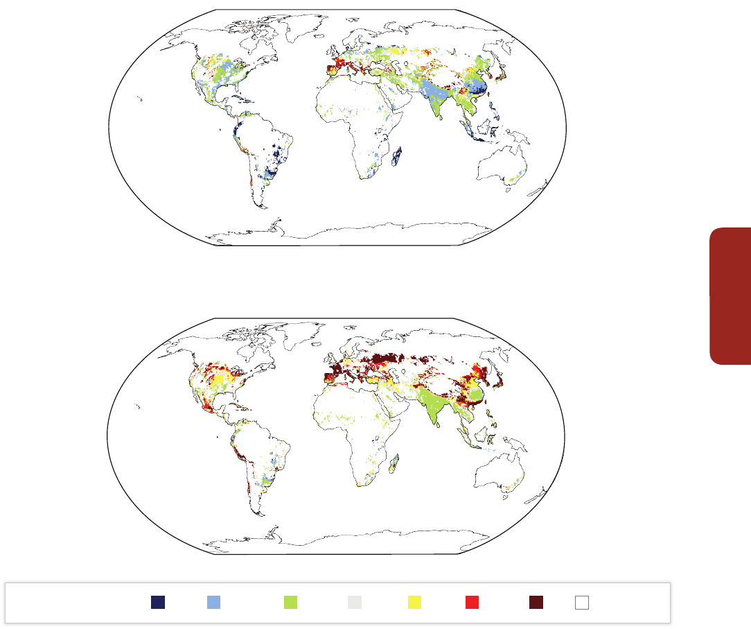
VW
Active Role of Vegetation in Altering Water Flows under Climate Change
Cross-Chapter Box
159
–20 to –40<–40 –5 to 20 –5 to 5 5 to 20 20 to 40 >40 No irrigation
(a) Impact of climate change including physiological and structural crop responses to increased
atmospheric CO
2
(b) Impact of climate change only
Percentage change in net
irrigation requirements
Figure VW-1 | Percentage change in net irrigation requirements of 11 major crops from 1971–2000 to 2070–2099 on areas currently equipped for irrigation, assuming current
management practices. (a) Impact of climate change including physiological and structural crop responses to increased atmospheric CO
2
concentration (co-limitation by nutrients
not considered). (b) Impact of climate change only. Shown is the median change derived from climate change projections by 19 General Circulation Models (GCMs; based on the
Special Report on Emission Scenarios (SRES) A2 emissions scenario) used to force a vegetation and hydrology model. (Modified after Konzmann et al., 2013.)
References
Alkama, R., M. Kageyama, and G. Ramstein, 2010: Relative contributions of climate change, stomatal closure, and leaf area index changes to 20th and 21st century
runoff change: a modelling approach using the Organizing Carbon and Hydrology in Dynamic Ecosystems (ORCHIDEE) land surface model. Journal of Geophysical
Research: Atmospheres, 115(D17), D17112, doi:10.1029/2009JD013408.
Alkama, R., B. Decharme, H. Douville, and A. Ribes, 2011: Trends in global and basin-scale runoff over the late twentieth century: methodological issues and sources of
uncertainty. Journal of Climate, 24(12), 3000-3014.
Anderegg, W.R.L., J.M. Kane, and L.D.L. Anderegg, 2013: Consequences of widespread tree mortality triggered by drought and temperature stress. Nature Climate
Change, 3, 30-36.
Andreu-Hayles, L., O. Planells, E. Gutierrez, E. Muntan, G. Helle, K.J. Anchukaitis, and G.H. Schleser, 2011: Long tree-ring chronologies reveal 20th century increases in
water-use efficiency but no enhancement of tree growth at five Iberian pine forests. Global Change Biology, 17(6), 2095-2112.

Cross-Chapter Box
Active Role of Vegetation in Altering Water Flows under Climate Change
160
VW
Betts, R.A., O. Boucher, M. Collins, P.M. Cox, P.D. Falloon, N. Gedney, D.L. Hemming, C. Huntingford, C.D. Jones, D.M.H. Sexton, and M.J. Webb, 2007: Projected increase in
continental runoff due to plant responses to increasing carbon dioxide. Nature, 448(7157), 1037-1041.
Boucher, O., A. Jones, and R.A. Betts, 2009: Climate response to the physiological impact of carbon dioxide on plants in the Met Office Unified Model HadCM3. Climate
Dynamics, 32(2-3), 237-249.
Brolsma, R.J., M.T.H. van Vliet, and M.F.P. Bierkens, 2010: Climate change impact on a groundwater-influenced hillslope ecosystem. Water Resources Research, 46(11),
W11503, doi:10.1029/2009WR008782.
Cao, L., G. Bala, K. Caldeira, R. Nemani, and G. Ban-Weiss, 2009: Climate response to physiological forcing of carbon dioxide simulated by the coupled Community
Atmosphere Model (CAM3.1) and Community Land Model (CLM3.0). Geophysical Research Letters, 36(10), L10402, doi:10.1029/2009GL037724.
Crosbie, R.S., J.L. McCallum, G.R. Walker, and F.H.S. Chiew, 2010: Modelling climate-change impacts on groundwater recharge in the Murray-Darling Basin, Australia.
Hydrogeology Journal, 18(7), 1639-1656.
Dai, A., T. Qian, K.E. Trenberth, and J.D. Milliman, 2009: Changes in continental freshwater discharge from 1948 to 2004. Journal of Climate, 22(10), 2773-2792.
Davie, J.C.S., P.D. Falloon, R. Kahana, R. Dankers, R. Betts, F.T. Portmann, D.B. Clark, A. Itoh, Y. Masaki, K. Nishina, B. Fekete, Z. Tessler, X. Liu, Q. Tang, S. Hagemann, T. Stacke,
R. Pavlick, S. Schaphoff, S.N. Gosling, W. Franssen, and N. Arnell, 2013: Comparing projections of future changes in runoff and water resources from hydrological and
ecosystem models in ISI-MIP. Earth System Dynamics, 4, 359-374.
de Boer, H.J., E.I. Lammertsma, F. Wagner-Cremer, D.L. Dilcher, M.J. Wassen, and S.C. Dekker, 2011: Climate forcing due to optimization of maximal leaf conductance in
subtropical vegetation under rising CO
2
. Proceedings of the National Academy of Sciences of the United States of America, 108(10), 4041-4046.
Donohue, R.J., M.L. Roderick, T.R. McVicar, and G.D. Farquhar, 2013: Impact of CO
2
fertilization on maximum foliage cover across the globe’s warm, arid environments.
Geophysical Research Letters, 40(12), 3031-3035.
Fader, M., S. Rost, C. Müller, A. Bondeau, and D. Gerten, 2010: Virtual water content of temperate cereals and maize: present and potential future patterns. Journal of
Hydrology, 384(3-4), 218-231.
Gagen, M., W. Finsinger, F. Wagner-Cremer, D. McCarroll, N.J. Loader, I. Robertson, R. Jalkanen, G. Young, and A. Kirchhefer, 2011: Evidence of changing intrinsic water-use
efficiency under rising atmospheric CO
2
concentrations in Boreal Fennoscandia from subfossil leaves and tree ring ∂
13
C ratios. Global Change Biology, 17(2), 1064-
1072.
Gedney, N., P.M. Cox, R.A. Betts, O. Boucher, C. Huntingford, and P.A. Stott, 2006: Detection of a direct carbon dioxide effect in continental river runoff records. Nature,
439(7078), 835-838.
Gerten, D., S. Rost, W. von Bloh, and W. Lucht, 2008: Causes of change in 20th century global river discharge. Geophysical Research Letters, 35(20), L20405,
doi:10.1029/2008GL035258.
Gerten, D., J. Heinke, H. Hoff, H. Biemans, M. Fader, and K. Waha, 2011: Global water availability and requirements for future food production. Journal of
Hydrometeorology, 12(5), 885-899.
Gerten, D., W. Lucht, S. Ostberg, J. Heinke, M. Kowarsch, H. Kreft, Z.W. Kundzewicz, J. Rastgooy, R. Warren, and H.J. Schellnhuber, 2013: Asynchronous exposure to global
warming: freshwater resources and terrestrial ecosystems. Environmental Research Letters, 8, 034032, doi:10.1088/1748-9326/8/3/034032.
Green, T.R., B.C. Bates, S.P. Charles, and P.M. Fleming, 2007: Physically based simulation of potential effects of carbon dioxide-altered climates on groundwater recharge.
Vadose Zone Journal, 6(3), 597-609.
Haddeland, I., D.B. Clark, W. Franssen, F. Ludwig, F. Voss, N.W. Arnell, N. Bertrand, M. Best, S. Folwell, D. Gerten, S. Gomes, S.N. Gosling, S. Hagemann, N. Hanasaki, R.
Harding, J. Heinke, P. Kabat, S. Koirala, T. Oki, J. Polcher, T. Stacke, P. Viterbo, G.P. Weedon, and P. Yeh, 2011: Multimodel estimate of the global terrestrial water
balance: setup and first results. Journal of Hydrometeorology, 12(5), 869-884.
Heyder, U., S. Schaphoff, D. Gerten, and W. Lucht, 2011: Risk of severe climate change impact on the terrestrial biosphere. Environmental Research Letters, 6(3), 034036,
doi:10.1088/1748-9326/6/3/034036.
Ito, A. and M. Inatomi, 2012: Water-use efficiency of the terrestrial biosphere: a model analysis focusing on interactions between the global carbon and water cycles.
Journal of Hydrometeorology, 13(2), 681-694.
Joshi, M.M., J.M. Gregory, M.J. Webb, D.M.H. Sexton, and T.C. Johns, 2008: Mechanisms for the land/sea warming contrast exhibited by simulations of climate change.
Climate Dynamics, 30(5), 455-465.
Keenan, T.F., D.Y. Hollinger, G. Bohrer, D. Dragoni, J.W. Munger, H.P. Schmid, and A.D. Richardson, 2013: Increase in forest water-use efficiency as atmospheric carbon
dioxide concentrations rise. Nature, 499(7458), 324-327.
Koehler, I.H., P.R. Poulton, K. Auerswald, and H. Schnyder, 2010: Intrinsic water-use efficiency of temperate seminatural grassland has increased since 1857: an analysis of
carbon isotope discrimination of herbage from the Park Grass Experiment. Global Change Biology, 16(5), 1531-1541.
Konzmann, M., D. Gerten, and J. Heinke, 2013: Climate impacts on global irrigation requirements under 19 GCMs, simulated with a vegetation and hydrology model.
Hydrological Sciences Journal, 58(1), 88-105.
Labat, D., Y. Godderis, J. Probst, and J. Guyot, 2004: Evidence for global runoff increase related to climate warming. Advances in Water Resources, 27(6), 631-642.
Leakey, A.D.B., E.A. Ainsworth, C.J. Bernacchi, A. Rogers, S.P. Long, and D.R. Ort, 2009: Elevated CO
2
effects on plant carbon, nitrogen, and water relations: six important
lessons from FACE. Journal of Experimental Botany, 60(10), 2859-2876.
Lewis, S.L., J. Lloyd, S. Sitch, E.T.A. Mitchard, and W.F. Laurance, 2009: Changing ecology of tropical forests: evidence and drivers. Annual Review of Ecology Evolution and
Systematics, 40, 529-549.
Loader, N.J., R.P.D. Walsh, I. Robertson, K. Bidin, R.C. Ong, G. Reynolds, D. McCarroll, M. Gagen, and G.H.F. Young, 2011: Recent trends in the intrinsic water-use efficiency
of ringless rainforest trees in Borneo. Philosophical Transactions of the Royal Society B, 366(1582), 3330-3339.
Lorenz, C. and H. Kunstmann, 2012: The hydrological cycle in three state-of-the-art reanalyses: intercomparison and performance analysis. Journal of Hydrometeorology,
13(5), 1397-1420.
McCallum, J.L., R.S. Crosbie, G.R. Walker, and W.R. Dawes, 2010: Impacts of climate change on groundwater in Australia: a sensitivity analysis of recharge. Hydrogeology
Journal, 18(7), 1625-1638.
McMahon, S.M., G.G. Parker, and D.R. Miller, 2010: Evidence for a recent increase in forest growth. Proceedings of the National Academy of Sciences of the United States
of America, 107(8), 3611-3615.
Murray, S.J., P.N. Foster, and I.C. Prentice, 2012: Future global water resources with respect to climate change and water withdrawals as estimated by a dynamic global
vegetation model. Journal of Hydrology, 448-449, 14-29.
Nock, C.A., P.J. Baker, W. Wanek, A. Leis, M. Grabner, S. Bunyavejchewin, and P. Hietz, 2011: Long-term increases in intrinsic water-use efficiency do not lead to increased
stem growth in a tropical monsoon forest in western Thailand. Global Change Biology, 17(2), 1049-1063.
Nugent, K.A. and H.D. Matthews, 2012: Drivers of future northern latitude runoff change. Atmosphere-Ocean, 50(2), 197-206.
Oliveira, P.J.C., E.L. Davin, S. Levis, and S.I. Seneviratne, 2011: Vegetation-mediated impacts of trends in global radiation on land hydrology: a global sensitivity study.
Global Change Biology, 17(11), 3453-3467.

VW
Active Role of Vegetation in Altering Water Flows under Climate Change
Cross-Chapter Box
161
Peñuelas, J., J.G. Canadell, and R. Ogaya, 2011: Increased water-use efficiency during the 20th century did not translate into enhanced tree growth. Global Ecology and
Biogeography, 20(4), 597-608.
Piao, S., P. Friedlingstein, P. Ciais, N. de Noblet-Ducoudre, D. Labat, and S. Zaehle, 2007: Changes in climate and land use have a larger direct impact than rising CO
2
on
global river runoff trends. Proceedings of the National Academy of Sciences of the United States of America, 104(39), 15242-15247.
Port, U., V. Brovkin, and M. Claussen, 2012: The influence of vegetation dynamics on anthropogenic climate change. Earth System Dynamics, 3, 233-243.
Reddy, A.R., G.K. Rasineni, and A.S. Raghavendra, 2010: The impact of global elevated CO
2
concentration on photosynthesis and plant productivity. Current Science,
99(1), 46-57.
Rosenthal, D.M. and N.J. Tomeo, 2013: Climate, crops and lacking data underlie regional disparities in the CO
2
fertilization effect. Environmental Research Letters, 8(3),
031001, doi:10.1088/1748-9326/8/3/031001.
Saatchi, S., S. Asefi-Najafabady, Y. Malhi, L.E.O.C. Aragão, L.O. Anderson, R.B. Myneni, and R. Nemani, 2013: Persistent effects of a severe drought on Amazonian forest
canopy. Proceedings of the National Academy of Sciences of the United States of America, 110(2), 565-570.
Sterling, S.M., A. Ducharne, and J. Polcher, 2013: The impact of global land-cover change on the terrestrial water cycle. Nature Climate Change, 3, 385-390.
Wiltshire, A., J. Gornall, B. Booth, E. Dennis, P. Falloon, G. Kay, D. McNeall, C. McSweeney, and R. Betts, 2013 : The importance of population, climate change and CO
2
plant
physiological forcing in determining future global water stress. Global Environmental Change, 23(5), 1083-1097.
Gerten, D., R. Betts, and P. Döll, 2014: Cross-chapter box on the active role of vegetation in altering water flows under climate change. In: Climate Change 2014:
Impacts, Adaptation, and Vulnerability. Part A: Global and Sectoral Aspects. Contribution of Working Group II to the Fifth Assessment Report of the Inter-
governmental Panel on Climate Change [Field, C.B., V.R. Barros, D.J. Dokken, K.J. Mach, M.D. Mastrandrea, T.E. Bilir, M. Chatterjee, K.L. Ebi, Y.O. Estrada, R.C.
Genova, B. Girma, E.S. Kissel, A.N. Levy, S. MacCracken, P.R. Mastrandrea, and L.L. White (eds.)]. Cambridge University Press, Cambridge, United Kingdom
and New York, NY, USA, pp. 157-161.
This cross-chapter box should be cited as:

The Water–Energy–Food/
Feed/Fiber Nexus as Linked
to Climate Change
Douglas J. Arent (USA), Petra Döll (Germany), Kenneth M. Strzepek (USA), Blanca Elena Jiménez
Cisneros (Mexico), Andy Reisinger (New Zealand), Ferenc Toth (Hungary), Taikan Oki (Japan)
WE
163
Water, energy, and food/feed/fiber are linked through numerous interactive pathways and
subject to a changing climate, as depicted in Figure CC-WE-1. The depth and intensity of those
linkages vary enormously among countries, regions, and production systems. Energy technologies
(e.g., biofuels, hydropower, thermal power plants), transportation fuels and modes, and food
products (from irrigated crops, in particular animal protein produced by feeding irrigated crops
and forages) may require significant amounts of water (Sections 3.7.2, 7.3.2, 10.2,10.3.4,
22.3.3, 25.7.2; Allan, 2003; King and Weber, 2008; McMahon and Price, 2011; Macknick et al.,
2012a). In irrigated agriculture, climate, irrigating procedure, crop choice, and yields determine
water requirements per unit of produced crop. In areas where water (and wastewater) must be
pumped and/or treated, energy must be provided (Metcalf & Eddy, Inc. et al., 2007; Khan and
Hanjra, 2009; EPA, 2010; Gerten et al., 2011). While food production, refrigeration, transport,
and processing require large amounts of energy (Pelletier et al., 2011), a major link between food
and energy as related to climate change is the competition of bioenergy and food production
for land and water (robust evidence, high agreement; Section 7.3.2, Box 25-10; Diffenbaugh et
al., 2012; Skaggs et al., 2012). Food and crop wastes, and wastewater, may be used as sources
of energy, saving not only the consumption of conventional nonrenewable fuels used in their
traditional processes, but also the consumption of the water and energy employed for processing
or treatment and disposal (Schievano et al., 2009; Oh et al., 2010; Olson, 2012). Examples of this
can be found in several countries across all income ranges. For example, sugar cane byproducts
are increasingly used to produce electricity or for cogeneration (McKendry, 2002; Kim and Dale,
2004) for economic benefits, and increasingly as an option for greenhouse gas mitigation.
Most energy production methods require significant amounts of water, either directly (e.g., crop-
based energy sources and hydropower) or indirectly (e.g., cooling for thermal energy sources or
other operations) (robust evidence, high agreement; Sections 10.2.2, 10.3.4, 25.7.4; and van Vliet
et al., 2012; Davies et al., 2013. Water for biofuels, for example, under the International Energy
Agency (IEA) Alternative Policy Scenario, which has biofuels production increasing to 71 EJ in
2030, has been reported by Gerbens-Leenes et al. (2012) to drive global consumptive irrigation
water use from 0.5% of global renewable water resources in 2005 to 5.5% in 2030, resulting
in increased pressure on freshwater resources, with potential negative impacts on freshwater
ecosystems. Water is also required for mining (Section 25.7.3), processing, and residue disposal of
fossil and nuclear fuels or their byproducts. Water for energy currently ranges from a few percent
in most developing countries to more than 50% of freshwater withdrawals in some developed
countries, depending on the country (Kenny et al., 2009; WEC, 2010). Future water requirements
will depend on electricity demand growth, the portfolio of generation technologies and water
management options employed (medium evidence, high agreement; WEC, 2010; Sattler et al.,
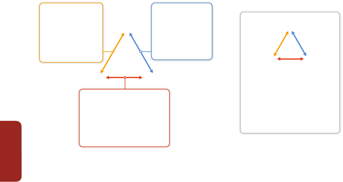
Cross-Chapter Box
The Water–Energy–Food/Feed/Fiber Nexus as Linked to Climate Change
164
WE
2012). Future water availability for energy production will change due to climate change (robust evidence, high agreement; Sections 3.4, 3.5.1,
3.5.2.2.
Water may require significant amounts of energy for lifting, transport, and distribution and for its treatment either to use it or to depollute it.
Wastewater and even excess rainfall in cities requires energy to be treated or disposed. Some non-conventional water sources (wastewater
or seawater) are often highly energy intensive. Energy intensities per m
3
of water vary by about a factor of 10 between different sources,
for example, locally produced potable water from ground/surface water sources versus desalinated seawater (Box 25-2, Tables 25-6, 25-7;
Macknick et al., 2012b; Plappally and Lienhard, 2012). Groundwater (35% of total global water withdrawals, with irrigated food production
being the largest user; Döll et al., 2012) is generally more energy intensive than surface water. In India, for example, 19% of total electricity
use in 2012 was for agricultural purposes (Central Statistics Office, 2013), with a large share for groundwater pumping. Pumping from greater
depth increases energy demand significantly—electricity use (kWh m
–3
of water) increases by a factor of 3 when going from 35 to 120 m depth
(Plappally and Lienhard, 2012). The reuse of appropriate wastewater for irrigation (reclaiming both water and energy-intense nutrients) may
increase agricultural yields, save energy, and prevent soil erosion (medium confidence; Smit and Nasr, 1992; Jiménez-Cisneros, 1996; Qadir et
al., 2007; Raschid-Sally and Jayakody, 2008). More energy efficient treatment methods enable poor quality (“black”) wastewater to be treated
to quality levels suitable for discharge into water courses, avoiding additional freshwater and associated energy demands (Keraita et al., 2008).
If properly treated to retain nutrients, such treated water may increase soil productivity, contributing to increased crop yields/food security in
regions unable to afford high power bills or expensive fertilizer (high confidence; Oron, 1996; Lazarova and Bahri, 2005; Redwood and Huibers,
2008; Jiménez-Cisneros, 2009).
Linkages among water, energy, food/feed/fiber, and climate are also strongly related to land use and management (robust evidence, high
agreement; Section 4.4.4, Box 25-10). Land degradation often reduces efficiency of water and energy use (e.g., resulting in higher fertilizer
demand and surface runoff), and compromises food security (Sections 3.7.2, 4.4.4). On the other hand, afforestation activities to sequester
carbon have important co-benefits of reducing soil erosion and providing additional (even if only temporary) habitat (see Box 25-10) but
may reduce renewable water resources. Water abstraction for energy, food, or biofuel production or carbon sequestration can also compete
with minimal environmental flows needed to maintain riverine habitats and wetlands, implying a potential conflict between economic and
other valuations and uses of water (medium evidence, high agreement; Sections 25.4.3, 25.6.2, Box 25-10). Only a few reports have begun to
evaluate the multiple interactions among energy, food, land, and water and climate (McCornick et al., 2008; Bazilian et al., 2011; Bierbaum and
Matson, 2013), addressing the issues from a security standpoint and describing early integrated modeling approaches. The interaction among
each of these factors is influenced by the changing climate, which in turn impacts energy and water demand, bioproductivity, and other factors
(see Figure CC-WE-1 and Wise et al., 2009), and has implications for security of supplies of energy, food, and water; adaptation and mitigation
pathways; and air pollution reduction, as well as the implications for health and economic impacts as described throughout this Assessment
Report.
Water
Energy Food/feed/fiber
Water for energy
• Cooling of thermal power plants
• Hydropower
• Irrigation of bioenergy crops
• Extraction and refining
Energy for water
• Extraction and transportation
• Water treatment/desalination
• Wastewater, drainage,
treatment, and disposal
Energy for food/feed/fiber
Energy – Water – Food/Feed/Fiber – Climate change
GHG
emissions/
climate change
Nutritionally appropriate low-meat diet or
low-water-consuming vegetarian diet
generally reduces water and energy demand
as well as GHG emissions per person.
Use of agricultural, livestock, and food waste
may reduce conventional energy use and GHG
emissions.
Climate change tends to increase energy
demand for cooling as well as water demand.
Figure WE-1
| The water–energy–food nexus as related to climate change. The interlinkages of supply/demand, quality and quantity of water, and energy and food/feed/fiber with
changing climatic conditions have implications for both adaptation and mitigation strategies.
• Crop and livestock production
• Processing and transport
• Food consumption
• Energy for irrigated crops
Food/feed/fiber for energy production
Competition between (bio)energy and
food/fiber production for water and land
Water for food/feed/fiber
Impact of food/feed/fiber
production on water
quality and runoff
generation
• Irrigation
• Livestock water use
• Water use for food processing

WE
The Water–Energy–Food/Feed/Fiber Nexus as Linked to Climate Change
Cross-Chapter Box
165
The interconnectivity of food/fiber, water, land use, energy, and climate change, including the perhaps not yet well understood cross-sector
impacts, are increasingly important in assessing the implications for adaptation/mitigation policy decisions. Fuel–food–land use–water–
greenhouse gas (GHG) mitigation strategy interactions, particularly related to bioresources for food/feed, power, or fuel, suggest that
combined assessment of water, land type, and use requirements, energy requirements, and potential uses and GHG impacts often epitomize
the interlinkages. For example, mitigation scenarios described in the IPCC Special Report on Renewable Energy Sources and Climate Change
Mitigation (IPCC, 2011) indicate up to 300 EJ of biomass primary energy by 2050 under increasingly stringent mitigation scenarios. Such high
levels of biomass production, in the absence of technology and process/management/operations change, would have significant implications
for land use, water, and energy, as well as food production and pricing. Consideration of the interlinkages of energy, food/feed/fiber, water,
land use, and climate change is increasingly recognized as critical to effective climate resilient pathway decision making (medium evidence,
high agreement), although tools to support local- and regional-scale assessments and decision support remain very limited.
References
Allan, T., 2003: Virtual water – the water, food, and trade nexus: useful concept or misleading metaphor? Water International, 28(1), 4-10.
Bazilian, M., H. Rogner, M. Howells, S. Hermann, D. Arent, D. Gielen, P. Steduto, A. Mueller, P. Komor, R.S.J. Tol, and K. Yumkella, 2011: Considering the energy, water and
food nexus: towards an integrated modelling approach. Energy Policy, 39(12), 7896-7906.
Bierbaum, R. and P. Matson, 2013: Energy in the context of sustainability. Daedalus, 142(1), 146-161.
Davies, E., K. Page, and J.A. Edmonds, 2013: An integrated assessment of global and regional water demands for electricity generation to 2095. Advances in Water
Resources, 52, 296-313, doi:10.1016/j.advwatres.2012.11.020.
Diffenbaugh, N., T. Hertel, M. Scherer, and M. Verma, 2012: Response of corn markets to climate volatility under alternative energy futures. Nature Climate Change, 2,
514-518.
Döll, P., H. Hoffmann-Dobrev, F.T. Portmann, S. Siebert, A. Eicker, M. Rodell, G. Strassberg, and B. Scanlon, 2012: Impact of water withdrawals from groundwater and
surface water on continental water storage variations. Journal of Geodynamics, 59-60, 143-156, doi:10.1016/j.jog.2011.05.001.
EPA, 2010: Evaluation of Energy Conservation Measures for Wastewater Treatment Facilities. EPA 832-R-10-005, U.S. Environmental Protection Agency (EPA), Office of
Wastewater Management, Washington, DC, USA, 222 pp., water.epa.gov/scitech/wastetech/upload/Evaluation-of-Energy-Conservation-Measures-for-Wastewater-
Treatment-Facilities.pdf.
Gerbens-Leenes, P.W., A.R. van Lienden, A.Y. Hoekstra, and Th.H. van der Meer, 2012: Biofuel scenarios in a water perspective: the global blue and green water footprint
of road transport in 2030. Global Environmental Change, 22(3), 764-775.
Gerber, N., M. van Eckert, and T. Breuer, 2008: The Impacts of Biofuel Production on Food Prices: A Review. ZEF – Discussion Papers on Development Policy, No. 127,
Center for Development Research [Zentrum für Entwicklungsforschung (ZEF)], Bonn, Germany, 19 pp.
Gerten, D., H. Heinke, H. Hoff, H. Biemans, M. Fader, and K. Waha, 2011: Global water availability and requirements for future food production. Journal of
Hydrometeorology, 12, 885-899.
IPCC, 2011: Summary for Policymakers. In: IPCC Special Report on Renewable Energy Sources and Climate Change Mitigation. Special Report of Working Group III of the
Intergovernmental Panel on Climate Change [Edenhofer, O., R. Pichs-Madruga, Y. Sokona, K. Seyboth, P. Matschoss, S. Kadner, T. Zwickel, P. Eickemeier, G. Hansen, S.
Schlmer, and C. von Stechow (eds.)]. Cambridge University Press, Cambridge, UK and New York, NY, USA, pp. 3-26.
Jiménez-Cisneros, B., 1996: Wastewater reuse to increase soil productivity. Water Science and Technology, 32(12), 173-180.
Jiménez-Cisneros, B., 2009: 4.06 – Safe sanitation in low economic development areas. In: Treatise on Water Science, Volume 4: Water-Quality Engineering [Wilderer,
P.A. (ed.)]. Reference Module in Earth Systems and Environmental Sciences, Academic Press, Oxford, UK, pp.147-200.
Kenny, J.F., N.L. Barber, S.S. Hutson, K.S. Linsey, J.K. Lovelace, and M.A. Maupin, 2009: Estimated Use of Water in the United States in 2005. U.S. Department of the Interior,
U.S. Geological Survey (USGS) Circular 1344, USGS, Reston, VA, USA, 53 pp.
Keraita, B., B. Jiménez, and P. Drechsel, 2008: Extent and implications of agricultural reuse of untreated, partly treated and diluted wastewater in developing countries.
CAB Reviews: Perspectives in Agriculture, Veterinary Science, Nutrition and Natural Resources, 3(58), 15-27.
Khan, S. and M.A. Hanjra, 2009: Footprints of water and energy inputs in food production – global perspectives. Food Policy, 34, 130-140.
Kim, S. and B. Dale, 2004: Global potential bioethanol production from wasted crops and crop residues. Biomass and Bioenergy, 26(4), 361-375.
King, C. and M.E. Webber, 2008: Water intensity of transportation. Environmental Science and Technology, 42(21), 7866-7872.
Lazarova, V. and A. Bahri, 2005: Water Reuse for Irrigation: Agriculture, Landscapes, and Turf Grass. CRC Press, Boca Raton, FL, USA, 408 pp.
McKendry, P., 2002: Energy production from biomass (part 1): overview of biomass. Bioresource Technology, 83(1), 37-46.
Macknick, J., R. Newmark, G. Heath, K.C. Hallett, J. Meldrum, and S. Nettles-Anderson, 2012a: Operational water consumption and withdrawal factors for electricity
generating technologies: a review of existing literature. Environmental Research Letters, 7(4), 045802, doi:10.1088/1748-9326/7/4/045802.
Macknick, J., S. Sattler, K. Averyt, S. Clemmer, and J. Rogers, 2012b: Water implications of generating electricity: water use across the United States based on different
electricity pathways through 2050. Environmental Research Letters, 7(4), 045803, doi:10.1088/1748-9326/7/4/045803.
McCornick, P.G., S.B. Awulachew, and M. Abebe, 2008: Water-food-energy-environment synergies and tradeoffs: major issues and case studies. Water Policy, 10, 23-36.
McMahon, J.E. and S.K. Price, 2011: Water and energy interactions. Annual Review of Environment and Resources, 36, 163-191.
Metcalf & Eddy, Inc. an AECOM Company, T. Asano, F. Burton, H. Leverenz, R. Tsuchihashi, and G. Tchobanoglous, 2007: Water Reuse: Issues, Technologies, and
Applications. McGraw-Hill Professional, New York, NY, USA, 1570 pp.
Oh, S.T., J.R. Kim, G.C. Premier, T.H. Lee, C. Kim, and W.T. Sloan, 2010: Sustainable wastewater treatment: how might microbial fuel cells contribute. Biotechnology
Advances, 28(6), 871-881.
Olson, G., 2012: Water and Energy Nexus: Threats and Opportunities. IWA Publishing, London, UK, 294 pp.
Oron, G., 1996: Soil as a complementary treatment component for simultaneous wastewater disposal and reuse. Water Science and Technology, 34(11), 243-252.
Pelletier, N., E. Audsley, S. Brodt, T. Garnett, P. Henriksson, A. Kendall, K.J. Kramer, D. Murphy, T. Nemeck, and M. Troell, 2011: Energy intensity of agriculture and food
systems. Annual Review of Environment and Resources, 36, 223-246.
Plappally, A.K. and J.H. Lienhard V, 2012: Energy requirements for water production, treatment, end use, reclamation, and disposal. Renewable and Sustainable Energy
Reviews, 16(7), 4818-4848.
Qadir, M., D. Wichelns, L. Raschid-Sally, P. Singh Minhas, P. Drechsel, A. Bahri, P. McCornick, R. Abaidoo, F. Attia, S. El-Guindy, J.H.J. Ensink, B. Jiménez, J.W. Kijne, S. Koo-
Oshima, J.D. Oster, L. Oyebande, J.A. Sagardoy, and W. van der Hoek, 2007: Agricultural use of marginal-quality water – opportunities and challenges. In: Water for
Food, Water for Life: A Comprehensive Assessment of Water Management in Agriculture [Molden, D. (ed.)]. Earthscan Publications, Ltd., London, UK, pp. 425-458.

Cross-Chapter Box
The Water-Energy-Food/Feed/Fiber Nexus as Linked to Climate Change
166
WE
Raschid-Sally, L. and P. Jayakody, 2008: Drivers and Characteristics of Wastewater Agriculture in Developing Countries: Results from a Global Assessment. IWMI
Research Report 127, International Water Management Institute (IWMI), Colombo, Sri Lanka, 29 pp.
Redwood, M. and F. Huibers, 2008: Wastewater irrigation in urban agriculture. In: Water Reuse: An International Survey of Current Practice, Issues and Needs [Jiménez, B.
and T. Asano (ed.)]. IWA Publishing, London, UK, pp. 228-240.
Sattler, S., J. Macknick, D. Yates, F. Flores-Lopez, A. Lopez, and J. Rogers, 2012: Linking electricity and water models to assess electricity choices at water-relevant scales.
Environmental Research Letters, 7(4), 045804, doi:10.1088/1748-9326/7/4/045804.
Schievano A., G. D’Imporzano, and F. Adani, 2009: Substituting energy crops with organic wastes and agro-industrial residues for biogas production. Journal of
Environmental Management, 90(8), 2537-2541.
Skaggs, R., K. Hibbard, P. Frumhoff, T. Lowry, R. Middleton, R. Pate, V. Tidwell, J. Arnold, K. Averyt, A. Janetos, C. Izaurralde, J. Rice, and S. Rose, 2012: Climate and Energy-
Water-Land System Interactions. PNNL 21185, Technical Report to the US Department of Energy in support of the National Climate Assessment, Pacific Northwest
National Laboratory (PNNL), Richland, WA, USA, 152 pp.
Smit, J. and J. Nasr, 1992: Urban agriculture for sustainable cities: using wastes and idle land and water bodies as resources. Environment and Urbanization, 4(2), 141-152.
van Vliet, M.T.H., J.R. Yearsley, F. Ludwig, S. Vögele, D.P. Lettenmaier, and P. Kabat, 2012: Vulnerability of US and European electricity supply to climate change. Nature
Climate Change, 2, 676-681.
Wise, M., K. Calvin, A. Thomson, L. Clarke, B. Bond-Lamberty, R. Sands, S.J. Smith, A. Janetos, and J. Edmonds, 2009: Implications of limiting CO
2
concentrations for land
use and energy. Science, 324, 1183-1186.
WEC, 2010: Water for Energy. World Energy Council (WEC), London, UK, 51 pp.
Arent, D.J., P. Döll, K.M. Strzepek, B.E. Jiménez Cisneros, A. Reisinger, F.L. Tóth, and T. Oki, 2014: Cross-chapter box on the water–energy–food/feed/fiber nexus
as linked to climate change. In: Climate Change 2014: Impacts, Adaptation, and Vulnerability. Part A: Global and Sectoral Aspects. Contribution of Working
Group II to the Fifth Assessment Report of the Intergovernmental Panel on Climate Change [Field, C.B., V.R. Barros, D.J. Dokken, K.J. Mach, M.D. Mastran-
drea, T.E. Bilir, M. Chatterjee, K.L. Ebi, Y.O. Estrada, R.C. Genova, B. Girma, E.S. Kissel, A.N. Levy, S. MacCracken, P.R. Mastrandrea, and L.L. White (eds.)].
Cambridge University Press, Cambridge, United Kingdom and New York, NY, USA, pp. 163-166.
This cross-chapter box should be cited as:
