
33
TS
This Technical Summary should be cited as:
Stocker, T.F., D. Qin, G.-K. Plattner, L.V. Alexander, S.K. Allen, N.L. Bindoff, F.-M. Bréon, J.A. Church, U. Cubasch,
S. Emori, P. Forster, P. Friedlingstein, N. Gillett, J.M. Gregory, D.L. Hartmann, E. Jansen, B. Kirtman, R. Knutti, K.
Krishna Kumar, P. Lemke, J. Marotzke, V. Masson-Delmotte, G.A. Meehl, I.I. Mokhov, S. Piao, V. Ramaswamy, D.
Randall, M. Rhein, M. Rojas, C. Sabine, D. Shindell, L.D. Talley, D.G. Vaughan and S.-P. Xie, 2013: Technical Sum-
mary. In: Climate Change 2013: The Physical Science Basis. Contribution of Working Group I to the Fifth Assess-
ment Report of the Intergovernmental Panel on Climate Change [Stocker, T.F., D. Qin, G.-K. Plattner, M. Tignor,
S.K. Allen, J. Boschung, A. Nauels, Y. Xia, V. Bex and P.M. Midgley (eds.)]. Cambridge University Press, Cambridge,
United Kingdom and New York, NY, USA.
Coordinating Lead Authors:
Thomas F. Stocker (Switzerland), Qin Dahe (China), Gian-Kasper Plattner (Switzerland)
Lead Authors:
Lisa V. Alexander (Australia), Simon K. Allen (Switzerland/New Zealand), Nathaniel L. Bindoff
(Australia), François-Marie Bréon (France), John A. Church (Australia), Ulrich Cubasch
(Germany), Seita Emori (Japan), Piers Forster (UK), Pierre Friedlingstein (UK/Belgium), Nathan
Gillett (Canada), Jonathan M. Gregory (UK), Dennis L. Hartmann (USA), Eystein Jansen (Norway),
Ben Kirtman (USA), Reto Knutti (Switzerland), Krishna Kumar Kanikicharla (India), Peter Lemke
(Germany), Jochem Marotzke (Germany), Valérie Masson-Delmotte (France), Gerald A. Meehl
(USA), Igor I. Mokhov (Russian Federation), Shilong Piao (China), Venkatachalam Ramaswamy
(USA), David Randall (USA), Monika Rhein (Germany), Maisa Rojas (Chile), Christopher Sabine
(USA), Drew Shindell (USA), Lynne D. Talley (USA), David G. Vaughan (UK), Shang-Ping Xie
(USA)
Contributing Authors:
Myles R. Allen (UK), Olivier Boucher (France), Don Chambers (USA), Jens Hesselbjerg
Christensen (Denmark), Philippe Ciais (France), Peter U. Clark (USA), Matthew Collins (UK),
Josefino C. Comiso (USA), Viviane Vasconcellos de Menezes (Australia/Brazil), Richard A. Feely
(USA), Thierry Fichefet (Belgium), Gregory Flato (Canada), Jesús Fidel González Rouco (Spain),
Ed Hawkins (UK), Paul J. Hezel (Belgium/USA), Gregory C. Johnson (USA), Simon A. Josey (UK),
Georg Kaser (Austria/Italy), Albert M.G. Klein Tank (Netherlands), Janina Körper (Germany),
Gunnar Myhre (Norway), Timothy Osborn (UK), Scott B. Power (Australia), Stephen R. Rintoul
(Australia), Joeri Rogelj (Switzerland/Belgium), Matilde Rusticucci (Argentina), Michael Schulz
(Germany), Jan Sedláček (Switzerland), Peter A. Stott (UK), Rowan Sutton (UK), Peter W. Thorne
(USA/Norway/UK), Donald Wuebbles (USA)
Review Editors:
Sylvie Joussaume (France), Joyce Penner (USA), Fredolin Tangang (Malaysia)
Technical Summary

TS
34
Table of Contents
TS.1 Introduction ........................................................................ 35
Box TS.1: Treatment of Uncertainty ........................................... 36
TS.2 Observation of Changes in the Climate System ...... 37
TS.2.1 Introduction ................................................................ 37
TS.2.2 Changes in Temperature.............................................. 37
TS.2.3 Changes in Energy Budget and Heat Content ............. 39
TS.2.4 Changes in Circulation and Modes of Variability ......... 39
TS.2.5 Changes in the Water Cycle and Cryosphere ............... 40
TS.2.6 Changes in Sea Level .................................................. 46
TS.2.7 Changes in Extremes ................................................... 46
TS.2.8 Changes in Carbon and Other
Biogeochemical Cycles ................................................ 50
TS.3 Drivers of Climate Change ............................................. 53
TS.3.1 Introduction ................................................................ 53
TS.3.2 Radiative Forcing from Greenhouse Gases .................. 53
Box TS.2: Radiative Forcing and Effective
Radiative Forcing ......................................................................... 53
TS.3.3 Radiative Forcing from Anthropogenic Aerosols .......... 55
TS.3.4 Radiative Forcing from Land Surface Changes
and Contrails ............................................................... 55
TS.3.5 Radiative Forcing from Natural Drivers of
Climate Change .......................................................... 55
TS.3.6 Synthesis of Forcings; Spatial and
Temporal Evolution ..................................................... 56
TS.3.7 Climate Feedbacks ...................................................... 57
TS.3.8 Emission Metrics ......................................................... 58
TS.4 Understanding the Climate System and
Its Recent Changes ........................................................... 60
TS.4.1 Introduction ................................................................ 60
TS.4.2 Surface Temperature ................................................... 60
Box TS.3: Climate Models and the Hiatus in Global
Mean Surface Warming of the Past 15 Years ............................ 61
TS.4.3 Atmospheric Temperature ........................................... 66
TS.4.4 Oceans ........................................................................ 68
TS.4.5 Cryosphere .................................................................. 69
TS.4.6 Water Cycle ................................................................. 72
TS.4.7 Climate Extremes ........................................................ 72
TS.4.8 From Global to Regional ............................................. 73
Box TS.4: Model Evaluation ........................................................ 75
Box TS.5: Paleoclimate ................................................................ 77
TS.5 Projections of Global and Regional
Climate Change.................................................................. 79
TS.5.1 Introduction ................................................................ 79
TS.5.2 Future Forcing and Scenarios ...................................... 79
Box TS.6: The New Representative Concentration Pathway
Scenarios and Coupled Model Intercomparison Project
Phase 5 Models ............................................................................ 79
TS.5.3 Quantification of Climate System Response ................ 81
TS.5.4 Near-term Climate Change ......................................... 85
TS.5.5 Long-term Climate Change ......................................... 89
TS.5.6 Long-term Projections of Carbon and Other
Biogeochemical Cycles ................................................ 93
Box TS.7: Climate Geoengineering Methods ............................ 98
TS.5.7 Long-term Projections of Sea Level Change ................ 98
TS.5.8 Climate Phenomena and Regional
Climate Change ........................................................ 105
TS.6 Key Uncertainties ............................................................ 114
TS.6.1 Key Uncertainties in Observation of Changes in
the Climate System ................................................... 114
TS.6.2 Key Uncertainties in Drivers of Climate Change ........ 114
TS.6.3 Key Uncertainties in Understanding the Climate
System and Its Recent Changes ................................ 114
TS.6.4 Key Uncertainties in Projections of Global and
Regional Climate Change .......................................... 115
Thematic Focus Elements
TFE.1 Water Cycle Change ................................................. 42
TFE.2 Sea Level Change: Scientific Understanding
and Uncertainties ..................................................... 47
TFE.3 Comparing Projections from Previous IPCC
Assessments with Observations ............................. 64
TFE.4 The Changing Energy Budget of the Global
Climate System ......................................................... 67
TFE.5 Irreversibility and Abrupt Change .......................... 70
TFE.6 Climate Sensitivity and Feedbacks ........................ 82
TFE.7 Carbon Cycle Perturbation and Uncertainties ...... 96
TFE.8 Climate Targets and Stabilization ........................ 102
TFE.9 Climate Extremes ................................................... 109
Supplementary Material
Supplementary Material is available in online versions of the report.

TS
Technical Summary
35
TS.1 Introduction
Climate Change 2013: The Physical Science Basis is the contribution
of Working Group I (WGI) to the Fifth Assessment Report (AR5) of the
Intergovernmental Panel on Climate Change (IPCC). This comprehen-
sive assessment of the physical aspects of climate change puts a focus
on those elements that are relevant to understand past, document cur-
rent and project future climate change. The assessment builds on the
IPCC Fourth Assessment Report (AR4)
1
and the recent Special Report
on Managing the Risk of Extreme Events and Disasters to Advance Cli-
mate Change Adaptation (SREX)
2
and is presented in 14 chapters and 3
annexes. The chapters cover direct and proxy observations of changes
in all components of the climate system; assess the current knowledge
of various processes within, and interactions among, climate system
components, which determine the sensitivity and response of the
system to changes in forcing; and quantify the link between the chang-
es in atmospheric constituents, and hence radiative forcing (RF)
3
, and
the consequent detection and attribution of climate change. Projec-
tions of changes in all climate system components are based on model
simulations forced by a new set of scenarios. The Report also provides
a comprehensive assessment of past and future sea level change in a
dedicated chapter. Regional climate change information is presented in
the form of an Atlas of Global and Regional Climate Projections (Annex
I). This is complemented by Annex II: Climate System Scenario Tables
and Annex III: Glossary.
The primary purpose of this Technical Summary (TS) is to provide the
link between the complete assessment of the multiple lines of inde-
pendent evidence presented in the 14 chapters of the main report
and the highly condensed summary prepared as the WGI Summary for
Policymakers (SPM). The Technical Summary thus serves as a starting
point for those readers who seek the full information on more specific
topics covered by this assessment. This purpose is facilitated by includ-
ing pointers to the chapters and sections where the full assessment
can be found. Policy-relevant topics, which cut across many chapters
and involve many interlinked processes in the climate system, are pre-
sented here as Thematic Focus Elements (TFEs), allowing rapid access
to this information.
An integral element of this report is the use of uncertainty language
that permits a traceable account of the assessment (Box TS.1). The
degree of certainty in key findings in this assessment is based on the
author teams’ evaluations of underlying scientific understanding and is
expressed as a level of confidence that results from the type, amount,
quality and consistency of evidence and the degree of agreement in
1
IPCC, 2007: Climate Change 2007: The Physical Science Basis. Contribution of Working Group I to the Fourth Assessment Report of the Intergovernmental Panel on Climate
Change [Solomon, S., D. Qin, M. Manning, Z. Chen, M. Marquis, K.B. Averyt, M. Tignor and H.L. Miller (eds.)]. Cambridge University Press, Cambridge, United Kingdom and New
York, NY, USA, 996 pp.
2
IPCC, 2012: Managing the Risks of Extreme Events and Disasters to Advance Climate Change Adaptation. A Special Report of Working Groups I and II of the Intergovernmental
Panel on Climate Change [Field, C.B., V. Barros, T.F. Stocker, D. Qin, D.J. Dokken, K.L. Ebi, M.D. Mastrandrea, K.J. Mach, G.-K. Plattner, S.K. Allen, M. Tignor and P. M. Midgley
(eds.)]. Cambridge University Press, Cambridge, UK, and New York, NY, USA, 582 pp.
3
Radiative forcing (RF) is a measure of the net change in the energy balance of the Earth system in response to some external perturbation. It is expressed in watts per square
metre (W m
–2
); see Box TS.2.
4
Mastrandrea, M.D., C.B. Field, T.F. Stocker, O. Edenhofer, K.L. Ebi, D.J. Frame, H. Held, E. Kriegler, K.J. Mach, P.R. Matschoss, G.-K. Plattner, G.W. Yohe, and F.W. Zwiers, 2010:
Guidance Note for Lead Authors of the IPCC Fifth Assessment Report on Consistent Treatment of Uncertainties. Intergovernmental Panel on Climate Change (IPCC).
the scientific studies considered
4
. Confidence is expressed qualita-
tively. Quantified measures of uncertainty in a finding are expressed
probabilistically and are based on a combination of statistical analy-
ses of observations or model results, or both, and expert judgement.
Where appropriate, findings are also formulated as statements of fact
without using uncertainty qualifiers (see Chapter 1 and Box TS.1 for
more details).
The Technical Summary is structured into four main sections presenting
the assessment results following the storyline of the WGI contribution
to AR5: Section TS.2 covers the assessment of observations of changes
in the climate system; Section TS.3 summarizes the information on
the different drivers, natural and anthropogenic, expressed in terms
of RF; Section TS.4 presents the assessment of the quantitative under-
standing of observed climate change; and Section TS.5 summarizes the
assessment results for projections of future climate change over the
21st century and beyond from regional to global scale. Section TS.6
combines and lists key uncertainties from the WGI assessment from
Sections TS.2 to TS.5. The overall nine TFEs, cutting across the various
components of the WGI AR5, are dispersed throughout the four main
TS sections, are visually distinct from the main text and should allow
stand-alone reading.
The basis for substantive paragraphs in this Technical Summary can be
found in the chapter sections of the underlying report. These references
are given in curly brackets.

TS
Technical Summary
36
Box TS.1 | Treatment of Uncertainty
Based on the Guidance Note for Lead Authors of the IPCC Fifth Assessment Report on Consistent Treatment of Uncertainties, this WGI
Technical Summary and the WGI Summary for Policymakers rely on two metrics for communicating the degree of certainty in key find-
ings, which is based on author teams’ evaluations of underlying scientific understanding:
• Confidence in the validity of a finding, based on the type, amount, quality and consistency of evidence (e.g., mechanistic under-
standing, theory, data, models, expert judgement) and the degree of agreement. Confidence is expressed qualitatively.
• Quantified measures of uncertainty in a finding expressed probabilistically (based on statistical analysis of observations or model
results, or expert judgement).
The AR5 Guidance Note refines the guidance provided to support the IPCC Third and Fourth Assessment Reports. Direct comparisons
between assessment of uncertainties in findings in this Report and those in the AR4 and the SREX are difficult, because of the applica-
tion of the revised guidance note on uncertainties, as well as the availability of new information, improved scientific understanding,
continued analyses of data and models and specific differences in methodologies applied in the assessed studies. For some climate
variables, different aspects have been assessed and therefore a direct comparison would be inappropriate.
Each key finding is based on an author team’s evaluation of associated evidence and agreement. The confidence metric provides a
qualitative synthesis of an author team’s judgement about the validity of a finding, as determined through evaluation of evidence and
agreement. If uncertainties can be quantified probabilistically, an author team can characterize a finding using the calibrated likelihood
language or a more precise presentation of probability. Unless otherwise indicated, high or very high confidence is associated with
findings for which an author team has assigned a likelihood term.
The following summary terms are used to describe the available evidence: limited, medium, or robust; and for the degree of agreement:
low, medium, or high. A level of confidence is expressed using five qualifiers very low, low, medium, high, and very high, and typeset
in italics, e.g., medium confidence. Box TS.1, Figure 1 depicts summary statements for evidence and agreement and their relationship
to confidence. There is flexibility in this relationship; for a given evidence and agreement statement, different confidence levels can be
assigned, but increasing levels of evidence and degrees of agreement correlate with increasing confidence.
High agreement
Limited evidence
High agreement
Medium evidence
High agreement
Robust evidence
Medium agreement
Robust evidence
Medium agreement
Medium evidence
Medium agreement
Limited evidence
Low agreement
Limited evidence
Low agreement
Medium evidence
Low agreement
Robust evidence
Evidence (type, amount, quality, consistency)
Agreement
Condence
Scale
Box TS.1, Figure 1 | A depiction of evidence and agreement statements and their relationship to confidence. Confidence increases toward the top right corner as
suggested by the increasing strength of shading. Generally, evidence is most robust when there are multiple, consistent independent lines of high quality. {Figure 1.11}
The following terms have been used to indicate the assessed likelihood, and typeset in italics:
Term* Likelihood of the outcome
Virtually certain 99–100% probability
Very likely 90–100% probability
Likely 66–100% probability
About as likely as not 33–66% probability
Unlikely 0–33% probability
Very unlikely 0–10% probability
Exceptionally unlikely 0–1% probability
* Additional terms (extremely likely: 95–100% probability, more likely than not: >50–100% probability, and extremely unlikely:
0–5% probability) may also be used when appropriate.

TS
Technical Summary
37
TS.2 Observation of Changes in the
Climate System
TS.2.1 Introduction
Observations of the climate system are based on direct physical and
biogeochemical measurements, and remote sensing from ground sta-
tions and satellites; information derived from paleoclimate archives
provides a long-term context. Global-scale observations from the
instrumental era began in the mid-19th century, and paleoclimate
reconstructions extend the record of some quantities back hundreds to
millions of years. Together, they provide a comprehensive view of the
variability and long-term changes in the atmosphere, the ocean, the
cryosphere and at the land surface.
The assessment of observational evidence for climate change is sum-
marized in this section. Substantial advancements in the availability,
acquisition, quality and analysis of observational data sets for the
atmosphere, land surface, ocean and cryosphere have occurred since
the AR4. Many aspects of the climate system are showing evidence of
a changing climate. {2, 3, 4, 5, 6, 13}
TS.2.2 Changes in Temperature
TS.2.2.1 Surface
It is certain that global mean surface temperature (GMST) has increased
since the late 19th century (Figures TS.1 and TS.2). Each of the past three
decades has been successively warmer at the Earth’s surface than any
the previous decades in the instrumental record, and the decade of the
2000’s has been the warmest. The globally averaged combined land and
ocean temperature data as calculated by a linear trend
5
, show a warm-
ing of 0.85 [0.65 to 1.06] °C
6
, over the period 1880–2012, when mul-
tiple independently produced datasets exist, about 0.89 [0.69 to 1.08]
°C over the period 1901–2012, and about 0.72 [0.49 to 0.89] °C over
the period 1951–2012 when based on three independently-produced
data sets. The total increase between the average of the 1850–1900
period and the 2003–2012 period is 0.78 [0.72 to 0.85] °C, based on
the Hadley Centre/Climatic Research Unit gridded surface temperature
data set 4 (HadCRUT4), the global mean surface temperature dataset
with the longest record of the three independently-produced data sets.
The warming from 1850–1900 to 1986–2005 (reference period for the
modelling chapters and the Atlas in Annex I) is 0.61 [0.55 to 0.67] °C,
when calculated using HadCRUT4 and its uncertainty estimates. It is
also virtually certain that maximum and minimum temperatures over
5
The warming is reported as an unweighted average based on linear trend estimates calculated from Hadley Centre/Climatic Research Unit gridded surface temperature data
set 4 (HadCRUT4), Merged Land–Ocean Surface Temperature Analysis (MLOST) and Goddard Institute for Space Studies Surface Temperature Analysis (GISTEMP) data sets
(see Figure TS.2; Section 2.4.3).
6
In the WGI contribution to the AR5, uncertainty is quantified using 90% uncertainty intervals unless otherwise stated. The 90% uncertainty interval, reported in square
brackets, is expected to have a 90% likelihood of covering the value that is being estimated. The upper endpoint of the uncertainty interval has a 95% likelihood of exceed-
ing the value that is being estimated and the lower endpoint has a 95% likelihood of being less than that value. A best estimate of that value is also given where available.
Uncertainty intervals are not necessarily symmetric about the corresponding best estimate.
7
Both methods presented in this paragraph to calculate temperature change were also used in AR4. The first calculates the difference using a best fit linear trend of all points
between two years, e.g., 1880 and 2012. The second calculates the difference between averages for the two periods, e.g., 1850 to 1900 and 2003 to 2012. Therefore, the
resulting values and their 90% uncertainty intervals are not directly comparable.
land have increased on a global scale since 1950.
7
{2.4.1, 2.4.3; Chapter
2 Supplementary Material Section 2.SM.3}
Despite the robust multi-decadal warming, there exists substantial
interannual to decadal variability in the rate of warming, with several
periods exhibiting weaker trends (including the warming hiatus since
1998) (Figure TS.1). The rate of warming over the past 15 years (1998–
2012; 0.05 [–0.05 to +0.15] °C per decade) is smaller than the trend
since 1951 (1951–2012; 0.12[0.08 to 0.14] °C per decade). Trends for
short periods are uncertain and very sensitive to the start and end
years. For example, trends for 15-year periods starting in 1995, 1996,
and 1997 are 0.13 [0.02 to 0.24] °C per decade, 0.14 [0.03 to 0.24]
°C per decade and 0.07 [–0.02 to 0.18] °C per decade, respectively.
Several independently analysed data records of global and regional
land surface air temperature obtained from station observations are
in broad agreement that land surface air temperatures have increased.
Sea surface temperatures (SSTs) have also increased. Intercomparisons
of new SST data records obtained by different measurement methods,
including satellite data, have resulted in better understanding of errors
and biases in the records. {2.4.1–2.4.3; Box 9.2}
It is unlikely that any uncorrected urban heat island effects and land
use change effects have raised the estimated centennial globally aver-
aged land surface air temperature trends by more than 10% of the
reported trend. This is an average value; in some regions that have
rapidly developed urban heat island and land use change impacts on
regional trends may be substantially larger. {2.4.1}
There is high confidence that annual mean surface warming since the
20th century has reversed long-term cooling trends of the past 5000
years in mid-to-high latitudes of the Northern Hemisphere (NH). For
average annual NH temperatures, the period 1983–2012 was very likely
the warmest 30-year period of the last 800 years (high confidence)
and likely the warmest 30-year period of the last 1400 years (medium
confidence). This is supported by comparison of instrumental tempera-
tures with multiple reconstructions from a variety of proxy data and
statistical methods, and is consistent with AR4. Continental-scale sur-
face temperature reconstructions show, with high confidence, multi-
decadal periods during the Medieval Climate Anomaly (950–1250)
that were in some regions as warm as in the mid-20th century and
in others as warm as in the late 20th century. With high confidence,
these regional warm periods were not as synchronous across regions
as the warming since the mid-20th century. Based on the comparison
between reconstructions and simulations, there is high confidence that
not only external orbital, solar and volcanic forcing, but also internal
TS
Technical Summary
38
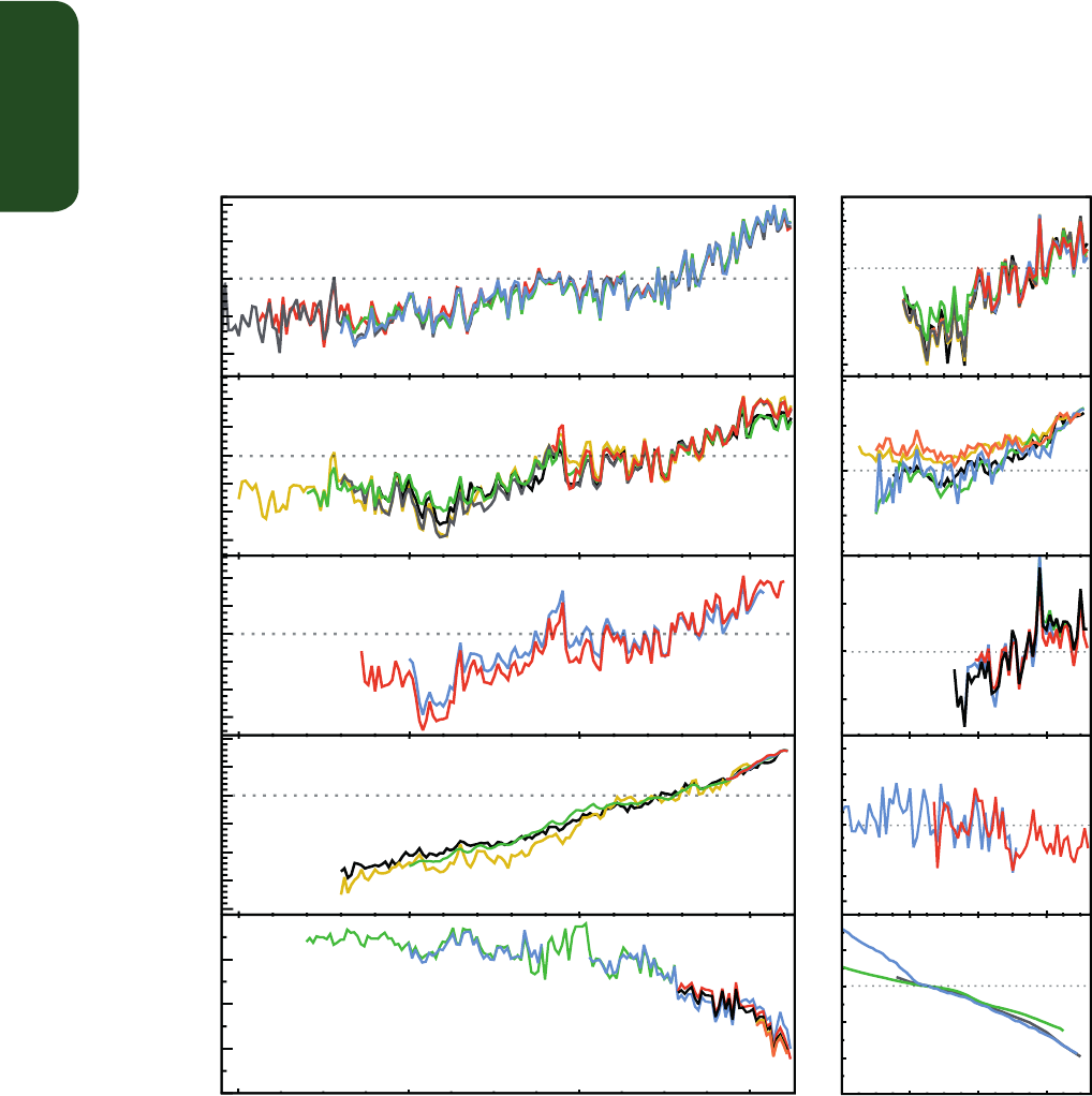
Figure TS.1 | Multiple complementary indicators of a changing global climate. Each line represents an independently derived estimate of change in the climate element. The times
series presented are assessed in Chapters 2, 3 and 4. In each panel all data sets have been normalized to a common period of record. A full detailing of which source data sets go
into which panel is given in Chapter 2 Supplementary Material Section 2.SM.5 and in the respective chapters. Further detail regarding the related Figure SPM.3 is given in the TS
Supplementary Material. {FAQ 2.1, Figure 1; 2.4, 2.5, 3.2, 3.7, 4.5.2, 4.5.3}
Land surface air temperature: 4 datasets
Mass balance (10
15
GT)
1.0
0.5
0.0
-0.5
-1.0
0.4
0.2
0.0
-0.2
-0.4
-0.6
0.4
0.2
0.0
-0.2
-0.4
-0.6
12
10
8
6
4
10
5
0
-5
-10
-15
0.4
0.2
0.0
-0.2
20
10
0
-10
0.6
0.4
0.2
0.0
-0.2
-0.4
-0.6
-0.8
100
50
0
-50
-100
-150
-200
Tropospheric temperature:
7 datasets
Ocean heat content(0-700m):
5 datasets
Specific humidity:
4 datasets
Glacier mass balance:
3 datasets
Sea-surface temperature: 5 datasets
Marine air temperature: 2 datasets
Sea level: 6 datasets
1850 1900 1950 2000
1940 1960 1980 2000
Summer arctic sea-ice extent: 6 datasets
Sea level
anomaly (mm)
Temperature
anomaly (ºC)
Temperature
anomaly (ºC)
Temperature
anomaly (ºC)
Temperature
anomaly (ºC)
Ocean heat content
anomaly (10
22
J)
Specific humidity
anomaly (g/kg)
Extent anomaly (10
6
km
2
)
6
4
2
0
-2
-4
-6
Extent (10
6
km
2
)
Year Year
Northern hemisphere (March-
April) snow cover: 2 datasets
variability, contributed substantially to the spatial pattern and timing
of surface temperature changes between the Medieval Climate Anom-
aly and the Little Ice Age (1450–1850). {5.3.5, 5.5.1}
TS.2.2.2 Troposphere and Stratosphere
Based on multiple independent analyses of measurements from radio-
sondes and satellite sensors, it is virtually certain that globally the
troposphere has warmed and the stratosphere has cooled since the
mid-20th century (Figure TS.1). Despite unanimous agreement on the
sign of the trends, substantial disagreement exists between available
estimates as to the rate of temperature changes, particularly outside
the NH extratropical troposphere, which has been well sampled by
radiosondes. Hence there is only medium confidence in the rate of
change and its vertical structure in the NH extratropical troposphere
and low confidence elsewhere. {2.4.4}
TS.2.2.3 Ocean
It is virtually certain that the upper ocean (above 700 m) has warmed
from 1971 to 2010, and likely that it has warmed from the 1870s to 1971
(Figure TS.1). There is less certainty in changes prior to 1971 because
of relatively sparse sampling in earlier time periods. Instrumental
biases in historical upper ocean temperature measurements have been
identified and reduced since AR4, diminishing artificial decadal varia-
tion in temperature and upper ocean heat content, most prominent
during the 1970s and 1980s. {3.2.1–3.2.3, 3.5.3}
TS
Technical Summary
39
Trend (ºC over period)
-0.6 -0.4 -0.2 00.2 0.40.6 0.811.25 1.5 1.75 2.5
HadCRUT4 1901-2012
MLOST 1901-2012
GISS 1901-2012
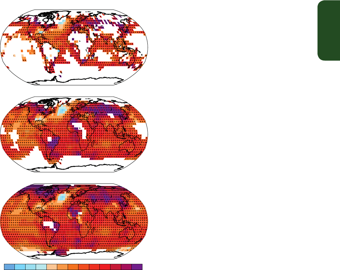
Figure TS.2 | Change in surface temperature over 1901–2012 as determined by linear
trend for three data sets. White areas indicate incomplete or missing data. Trends have
been calculated only for those grid boxes with greater than 70% complete records and
more than 20% data availability in the first and last 10% of the time period. Black plus
signs (+) indicate grid boxes where trends are significant (i.e., a trend of zero lies out-
side the 90% confidence interval). Differences in coverage primarily reflect the degree
of interpolation to account for data void regions undertaken by the data set providers
ranging from none beyond grid box averaging (Hadley Centre/Climatic Research Unit
gridded surface temperature data set 4 (HadCRUT4)) to substantial (Goddard Institute
for Space Studies Surface Temperature Analysis (GISTEMP)). Further detail regarding the
related Figure SPM.1 is given in the TS Supplementary Material. {Figure 2.21}
It is likely that the ocean warmed between 700-2000 m from 1957 to
2009, based on 5-year averages. It is likely that the ocean warmed from
3000 m to the bottom from 1992 to 2005, while no significant trends
in global average temperature were observed between 2000 and 3000
m depth from circa 1992 to 2005. Below 3000 m depth, the largest
warming is observed in the Southern Ocean. {3.2.4, 3.5.1; Figures 3.2b,
3.3; FAQ 3.1}
TS.2.3 Changes in Energy Budget and Heat Content
The Earth has been in radiative imbalance, with more energy from the
Sun entering than exiting the top of the atmosphere, since at least
about 1970. It is virtually certain that the Earth has gained substantial
energy from 1971 to 2010. The estimated increase in energy inventory
between 1971 and 2010 is 274 [196 to 351] × 10
21
J (high confidence),
with a heating rate of 213 × 10
12
W from a linear fit to the annual
values over that time period (see also TFE.4). {Boxes 3.1, 13.1}
Ocean warming dominates that total heating rate, with full ocean
depth warming accounting for about 93% (high confidence), and
warming of the upper (0 to 700 m) ocean accounting for about 64%.
Melting ice (including Arctic sea ice, ice sheets and glaciers) and warm-
ing of the continents each account for 3% of the total. Warming of the
atmosphere makes up the remaining 1%. The 1971–2010 estimated
rate of ocean energy gain is 199 × 10
12
W from a linear fit to data over
that time period, equivalent to 0.42 W m
–2
heating applied continu-
ously over the Earth’s entire surface, and 0.55 W m
–2
for the portion
owing to ocean warming applied over the ocean’s entire surface area.
The Earth’s estimated energy increase from 1993 to 2010 is 163 [127
to 201] × 10
21
J with a trend estimate of 275 × 10
15
W. The ocean por-
tion of the trend for 1993–2010 is 257 × 10
12
W, equivalent to a mean
heat flux into the ocean of 0.71 W m
–2
. {3.2.3, 3.2.4; Box 3.1}
It is about as likely as not that ocean heat content from 0–700 m
increased more slowly during 2003 to 2010 than during 1993 to 2002
(Figure TS.1). Ocean heat uptake from 700–2000 m, where interannual
variability is smaller, likely continued unabated from 1993 to 2009.
{3.2.3, 3.2.4; Box 9.2}
TS.2.4 Changes in Circulation and Modes of Variability
Large variability on interannual to decadal time scales hampers robust
conclusions on long-term changes in atmospheric circulation in many
instances. Confidence is high that the increase of the northern mid-
latitude westerly winds and the North Atlantic Oscillation (NAO) index
from the 1950s to the 1990s, and the weakening of the Pacific Walker
Circulation from the late 19th century to the 1990s, have been largely
offset by recent changes. With high confidence, decadal and multi-
decadal changes in the winter NAO index observed since the 20th cen-
tury are not unprecedented in the context of the past 500 years. {2.7.2,
2.7.5, 2.7.8, 5.4.2; Box 2.5; Table 2.14}
It is likely that circulation features have moved poleward since the
1970s, involving a widening of the tropical belt, a poleward shift of
storm tracks and jet streams and a contraction of the northern polar
vortex. Evidence is more robust for the NH. It is likely that the Southern
Annular Mode (SAM) has become more positive since the 1950s. The
increase in the strength of the observed summer SAM since 1950 has
been anomalous, with medium confidence, in the context of the past
400 years. {2.7.5, 2.7.6, 2.7.8, 5.4.2; Box 2.5; Table 2.14}
New results from high-resolution coral records document with high
confidence that the El Niño-Southern Oscillation (ENSO) system has
remained highly variable throughout the past 7000 years, showing no
discernible evidence for an orbital modulation of ENSO. {5.4.1}

TS
Technical Summary
40
Recent observations have strengthened evidence for variability in
major ocean circulation systems on time scales from years to decades.
It is very likely that the subtropical gyres in the North Pacific and
South Pacific have expanded and strengthened since 1993. Based on
measurements of the full Atlantic Meridional Overturning Circulation
(AMOC) and its individual components at various latitudes and differ-
ent time periods, there is no evidence of a long-term trend. There is also
no evidence for trends in the transports of the Indonesian Throughflow,
the Antarctic Circumpolar Current (ACC) or in the transports between
the Atlantic Ocean and Nordic Seas. However, a southward shift of the
ACC by about 1° of latitude is observed in data spanning the time
period 1950–2010 with medium confidence. {3.6}
TS.2.5 Changes in the Water Cycle and Cryosphere
TS.2.5.1 Atmosphere
Confidence in precipitation change averaged over global land areas
is low prior to 1951 and medium afterwards because of insufficient
data, particularly in the earlier part of the record (for an overview of
observed and projected changes in the global water cycle see TFE.1).
Further, when virtually all the land area is filled in using a reconstruc-
tion method, the resulting time series shows little change in land-
based precipitation since 1901. NH mid-latitude land areas do show
a likely overall increase in precipitation (medium confidence prior to
1951, but high confidence afterwards). For other latitudes area-aver-
aged long-term positive or negative trends have low confidence (TFE.1,
Figure 1). {2.5.1}
It is very likely that global near surface and tropospheric air specif-
ic humidity have increased since the 1970s. However, during recent
years the near-surface moistening trend over land has abated (medium
confidence) (Figure TS.1). As a result, fairly widespread decreases in
relative humidity near the surface are observed over the land in recent
years. {2.4.4, 2.5.5, 2.5.6}
Although trends of cloud cover are consistent between independent
data sets in certain regions, substantial ambiguity and therefore low
confidence remains in the observations of global-scale cloud variability
and trends. {2.5.7}
TS.2.5.2 Ocean and Surface Fluxes
It is very likely that regional trends have enhanced the mean geograph-
ical contrasts in sea surface salinity since the 1950s: saline surface
waters in the evaporation-dominated mid-latitudes have become more
saline, while relatively fresh surface waters in rainfall-dominated tropi-
cal and polar regions have become fresher. The mean contrast between
high- and low-salinity regions increased by 0.13 [0.08 to 0.17] from
1950 to 2008. It is very likely that the inter-basin contrast in freshwater
content has increased: the Atlantic has become saltier and the Pacific
and Southern Oceans have freshened. Although similar conclusions
were reached in AR4, recent studies based on expanded data sets and
new analysis approaches provide high confidence in this assessment.
{3.3.2, 3.3.3, 3.9; FAQ 3.2}
The spatial patterns of the salinity trends, mean salinity and the mean
distribution of evaporation minus precipitation are all similar (TFE.1,
Figure 1). These similarities provide indirect evidence that the pattern
of evaporation minus precipitation over the oceans has been enhanced
since the 1950s (medium confidence). Uncertainties in currently avail-
able surface fluxes prevent the flux products from being reliably used
to identify trends in the regional or global distribution of evaporation
or precipitation over the oceans on the time scale of the observed salin-
ity changes since the 1950s. {3.3.2–3.3.4, 3.4.2, 3.4.3, 3.9; FAQ 3.2}
TS.2.5.3 Sea Ice
Continuing the trends reported in AR4, there is very high confidence
that the Arctic sea ice extent (annual, multi-year and perennial)
decreased over the period 1979–2012 (Figure TS.1). The rate of the
annual decrease was very likely between 3.5 and 4.1% per decade
(range of 0.45 to 0.51 million km
2
per decade). The average decrease in
decadal extent of annual Arctic sea ice has been most rapid in summer
and autumn (high confidence), but the extent has decreased in every
season, and in every successive decade since 1979 (high confidence).
The extent of Arctic perennial and multi-year ice decreased between
1979 and 2012 (very high confidence). The rates are very likely 11.5
[9.4 to 13.6]% per decade (0.73 to 1.07 million km
2
per decade) for the
sea ice extent at summer minimum (perennial ice) and very likely 13.5
[11 to 16] % per decade for multi-year ice. There is medium confidence
from reconstructions that the current (1980–2012) Arctic summer sea
ice retreat was unprecedented and SSTs were anomalously high in the
perspective of at least the last 1,450 years. {4.2.2, 5.5.2}
It is likely that the annual period of surface melt on Arctic perennial
sea ice lengthened by 5.7 [4.8 to 6.6] days per decade over the period
1979–2012. Over this period, in the region between the East Siberian
Sea and the western Beaufort Sea, the duration of ice-free conditions
increased by nearly 3 months. {4.2.2}
There is high confidence that the average winter sea ice thickness
within the Arctic Basin decreased between 1980 and 2008. The aver-
age decrease was likely between 1.3 m and 2.3 m. High confidence in
this assessment is based on observations from multiple sources: sub-
marine, electromagnetic probes and satellite altimetry; and is consistent
with the decline in multi-year and perennial ice extent. Satellite mea-
surements made in the period 2010–2012 show a decrease in sea ice
volume compared to those made over the period 2003–2008 (medium
confidence). There is high confidence that in the Arctic, where the sea
ice thickness has decreased, the sea ice drift speed has increased. {4.2.2}
It is very likely that the annual Antarctic sea ice extent increased at a
rate of between 1.2 and 1.8% per decade (0.13 to 0.20 million km
2
per decade) between 1979 and 2012 (very high confidence). There was
a greater increase in sea ice area, due to a decrease in the percent-
age of open water within the ice pack. There is high confidence that
there are strong regional differences in this annual rate, with some
regions increasing in extent/area and some decreasing. There are also
contrasting regions around the Antarctic where the ice-free season has
lengthened, and others where it has decreased over the satellite period
(high confidence). {4.2.3}
TS
Technical Summary
41
TS.2.5.4 Glaciers and Ice Sheets
There is very high confidence that glaciers world-wide are persistently
shrinking as revealed by the time series of measured changes in glacier
length, area, volume and mass (Figures TS.1 and TS.3). The few excep-
tions are regionally and temporally limited. Measurements of glacier
change have increased substantially in number since AR4. Most of the
new data sets, along with a globally complete glacier inventory, have
been derived from satellite remote sensing {4.3.1, 4.3.3}
There is very high confidence that, during the last decade, the largest
contributions to global glacier ice loss were from glaciers in Alaska, the
Canadian Arctic, the periphery of the Greenland ice sheet, the South-
ern Andes and the Asian mountains. Together these areas account for
more than 80% of the total ice loss. Total mass loss from all glaciers
in the world, excluding those on the periphery of the ice sheets, was
very likely 226 [91 to 361] Gt yr
–1
(sea level equivalent, 0.62 [0.25 to
0.99] mm yr
–1
) in the period 1971–2009, 275 [140 to 410] Gt yr
–1
(0.76
[0.39 to 1.13] mm yr
–1
) in the period 1993–2009 and 301 [166 to 436]
Gt yr
–1
(0.83 [0.46 to 1.20] mm yr
–1
) between 2005 and 2009
8
. {4.3.3;
Tables 4.4, 4.5}
8
100 Gt yr
–1
of ice loss corresponds to about 0.28 mm yr
–1
of sea level equivalent.
There is high confidence that current glacier extents are out of balance
with current climatic conditions, indicating that glaciers will continue to
shrink in the future even without further temperature increase. {4.3.3}
There is very high confidence that the Greenland ice sheet has lost ice
during the last two decades. Combinations of satellite and airborne
remote sensing together with field data indicate with high confidence
that the ice loss has occurred in several sectors and that large rates of
mass loss have spread to wider regions than reported in AR4 (Figure
TS.3). There is high confidence that the mass loss of the Greenland
ice sheet has accelerated since 1992: the average rate has very likely
increased from 34 [–6 to 74] Gt yr
–1
over the period 1992–2001 (sea
level equivalent, 0.09 [–0.02 to 0.20] mm yr
–1
), to 215 [157 to 274] Gt
yr
–1
over the period 2002–2011 (0.59 [0.43 to 0.76] mm yr
–1
). There is
high confidence that ice loss from Greenland resulted from increased
surface melt and runoff and increased outlet glacier discharge, and
these occurred in similar amounts. There is high confidence that the
area subject to summer melt has increased over the last two decades.
{4.4.2, 4.4.3}
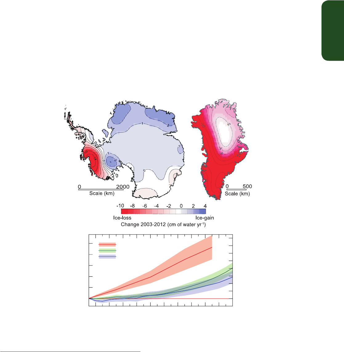
Figure TS.3 | (Upper) Distribution of ice loss determined from Gravity Recovery and Climate Experiment (GRACE) time-variable gravity for (a) Antarctica and (b) Greenland, shown
in centimetres of water per year (cm of water yr
–1
) for the period 2003–2012. (Lower) The assessment of the total loss of ice from glaciers and ice sheets in terms of mass (Gt) and
sea level equivalent (mm). The contribution from glaciers excludes those on the periphery of the ice sheets. {4.3.4; Figures 4.12–4.14, 4.16, 4.17, 4.25}
(a) (b)
1992 1994 1996 1998 2000 2002 2004 2006 2008 2010 2012
Year
Glaciers
Greenland
Antarctica
-2
0
2
4
6
8
10
12
14
16
SLE (mm)
0
1000
2000
3000
4000
5000
Cumulative ice mass loss (Gt)

TS
Technical Summary
42
Thematic Focus Elements
TFE.1 | Water Cycle Change
The water cycle describes the continuous movement of water through the climate system in its liquid, solid and
vapour forms, and storage in the reservoirs of ocean, cryosphere, land surface and atmosphere. In the atmosphere,
water occurs primarily as a gas, water vapour, but it also occurs as ice and liquid water in clouds. The ocean is pri-
marily liquid water, but the ocean is partly covered by ice in polar regions. Terrestrial water in liquid form appears
as surface water (lakes, rivers), soil moisture and groundwater. Solid terrestrial water occurs in ice sheets, glaciers,
snow and ice on the surface and permafrost. The movement of water in the climate system is essential to life on
land, as much of the water that falls on land as precipitation and supplies the soil moisture and river flow has been
evaporated from the ocean and transported to land by the atmosphere. Water that falls as snow in winter can
provide soil moisture in springtime and river flow in summer and is essential to both natural and human systems.
The movement of fresh water between the atmosphere and the ocean can also influence oceanic salinity, which is
an important driver of the density and circulation of the ocean. The latent heat contained in water vapour in the
atmosphere is critical to driving the circulation of the atmosphere on scales ranging from individual thunderstorms
to the global circulation of the atmosphere. {12.4.5; FAQ 3.2, FAQ 12.2}
Observations of Water Cycle Change
Because the saturation vapour pressure of air increases with temperature, it is expected that the amount of water
vapour in air will increase with a warming climate. Observations from surface stations, radiosondes, global posi-
tioning systems and satellite measurements indicate increases in tropospheric water vapour at large spatial scales
(TFE.1, Figure 1). It is very likely that tropospheric specific humidity has increased since the 1970s. The magnitude
of the observed global change in tropospheric water vapour of about 3.5% in the past 40 years is consistent with
the observed temperature change of about 0.5°C during the same period, and the relative humidity has stayed
approximately constant. The water vapour change can be attributed to human influence with medium confidence.
{2.5.4, 10.3.2}
Changes in precipitation are harder to measure with the existing records, both because of the greater difficulty
in sampling precipitation and also because it is expected that precipitation will have a smaller fractional change
than the water vapour content of air as the climate warms. Some regional precipitation trends appear to be robust
(TFE.1, Figure 2), but when virtually all the land area is filled in using a reconstruction method, the resulting time
series of global mean land precipitation shows little change since 1900. At present there is medium confidence that
there has been a significant human influence on global scale changes in precipitation patterns, including increases
in Northern Hemisphere (NH) mid-to-high latitudes. Changes in the extremes of precipitation, and other climate
extremes related to the water cycle are comprehensively discussed in TFE.9. {2.5.1, 10.3.2}
Although direct trends in precipitation and evaporation are difficult to measure with the available records, the
observed oceanic surface salinity, which is strongly dependent on the difference between evaporation and pre-
cipitation, shows significant trends (TFE.1, Figure 1). The spatial patterns of the salinity trends since 1950 are very
similar to the mean salinity and the mean distribution of evaporation minus precipitation: regions of high salinity
where evaporation dominates have become more saline, while regions of low salinity where rainfall dominates
have become fresher (TFE.1, Figure 1). This provides indirect evidence that the pattern of evaporation minus pre-
cipitation over the oceans has been enhanced since the 1950s (medium confidence). The inferred changes in evapo-
ration minus precipitation are consistent with the observed increased water vapour content of the warmer air. It is
very likely that observed changes in surface and subsurface salinity are due in part to anthropogenic climate forc-
ings. {2.5, 3.3.2–3.3.4, 3.4, 3.9, 10.4.2; FAQ 3.2}
In most regions analysed, it is likely that decreasing numbers of snowfall events are occurring where increased
winter temperatures have been observed. Both satellite and in situ observations show significant reductions in
the NH snow cover extent over the past 90 years, with most of the reduction occurring in the 1980s. Snow cover
decreased most in June when the average extent decreased very likely by 53% (40 to 66%) over the period 1967
to 2012. From 1922 to 2012 only data from March and April are available and show very likely a 7% (4.5 to 9.5%)
decline. Because of earlier spring snowmelt, the duration of the NH snow season has declined by 5.3 days per
decade since the 1972/1973 winter. It is likely that there has been an anthropogenic component to these observed
reductions in snow cover since the 1970s. {4.5.2, 10.5.1, 10.5.3}
(continued on next page)
TS
Technical Summary
43
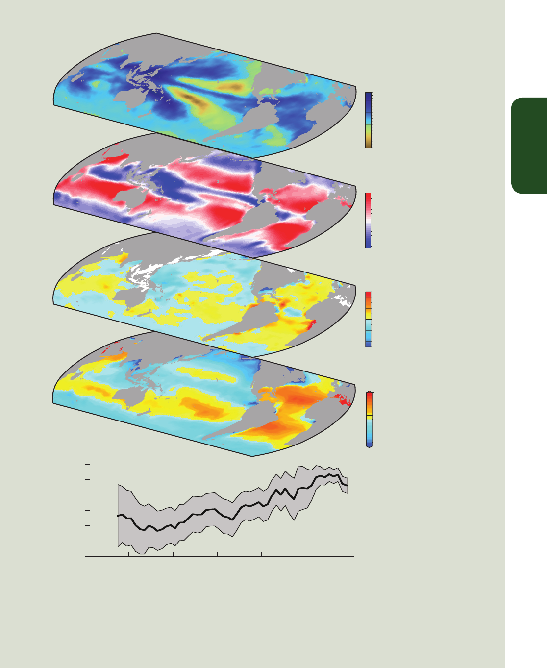
TFE.1, Figure 1 | Changes in sea surface salinity are related to the atmospheric patterns of evaporation minus precipitation (E – P) and trends in total precipitable
water: (a) Linear trend (1988 to 2010) in total precipitable water (water vapour integrated from the Earth’s surface up through the entire atmosphere) (kg m
–2
per
decade) from satellite observations. (b) The 1979–2005 climatological mean net evaporation minus precipitation (cm yr
–1
) from meteorological reanalysis data. (c) Trend
(1950–2000) in surface salinity (Practical Salinity Scale 78 (PSS78) per 50 years). (d) The climatological mean surface salinity (PSS78) (blues <35; yellows-reds >35). (e)
Global difference between salinity averaged over regions where the sea surface salinity is greater than the global mean sea surface salinity (“High Salinity”) and salinity
averaged over regions with values below the global mean (‘Low Salinity’). For details of data sources see Figure 3.21 and FAQ 3.2, Figure 1. {3.9}
TFE.1 (continued)
(e) High salinity
minus low Salinity
1950 1960 1970 1980 1990 2000 2010
-0.09
-0.06
-0.03
0
0.03
0.06
0.09
∆salinity (PSS78)
Year
31
33
35
37
(d) Mean
surface salinity
(PSS78)
−0.8
−0.4
0.0
0.4
0.8
(c) Trend in
surface salinity
(1950-2000)
(PSS78 per decade)
−100
0
100
(b) Mean
evaporation
minus
precipitation
(cm yr
-1
)
−1.6
−0.8
0.0
0.8
1.6
(a) Trend in
total precipitable
water vapour
(1988-2010)
(kg m
-2
per decade)
TS
Technical Summary
44
The most recent and most comprehensive analyses of river runoff do not support the IPCC Fourth Assessment Report
(AR4) conclusion that global runoff has increased during the 20th century. New results also indicate that the AR4
conclusions regarding global increasing trends in droughts since the 1970s are no longer supported. {2.5.2, 2.6.2}
Projections of Future Changes
Changes in the water cycle are projected to occur in a warming climate (TFE.1, Figure 3, see also TS 4.6, TS 5.6,
Annex I). Global-scale precipitation is projected to gradually increase in the 21st century. The precipitation increase
is projected to be much smaller (about 2% K
–1
) than the rate of lower tropospheric water vapour increase (about
7% K
–1
), due to global energetic constraints. Changes of average precipitation in a much warmer world will not be
uniform, with some regions experiencing increases, and others with decreases or not much change at all. The high
latitude land masses are likely to experience greater amounts of precipitation due to the additional water carrying
capacity of the warmer troposphere. Many mid-latitude and subtropical arid and semi-arid regions will likely experi-
ence less precipitation. The largest precipitation changes over northern Eurasia and North America are projected to
occur during the winter. {12.4.5, Annex I}
(continued on next page)
TFE.1 (continued)
TFE.1, Figure 2 | Maps of observed precipitation change over land from 1901 to 2010 (left-hand panels) and 1951 to 2010 (right-hand panels) from the Climatic
Research Unit (CRU), Global Historical Climatology Network (GHCN) and Global Precipitation Climatology Centre (GPCC) data sets. Trends in annual accumulation have
been calculated only for those grid boxes with greater than 70% complete records and more than 20% data availability in first and last decile of the period. White areas
indicate incomplete or missing data. Black plus signs (+) indicate grid boxes where trends are significant (i.e., a trend of zero lies outside the 90% confidence interval).
Further detail regarding the related Figure SPM.2 is given in the TS Supplementary Material. {Figure 2.29; 2.5.1}
Trend (mm yr
-1
per decade)
CRU 1901-2010
GHCN 1901-2010 GHCN 1951-2010
GPCC 1901-2010 GPCC 1951-2010
CRU 1951-2010
-100 -50 -25 -10 -5 -2.5 0 2.5 5102550 100
TS
Technical Summary
45
Regional to global-scale projections of soil moisture and drought remain relatively uncertain compared to other
aspects of the water cycle. Nonetheless, drying in the Mediterranean, southwestern USA and southern African
regions are consistent with projected changes in the Hadley Circulation, so drying in these regions as global temper-
atures increase is likely for several degrees of warming under the Representative Concentration Pathway RCP8.5.
Decreases in runoff are likely in southern Europe and the Middle East. Increased runoff is likely in high northern
latitudes, and consistent with the projected precipitation increases there. {12.4.5}
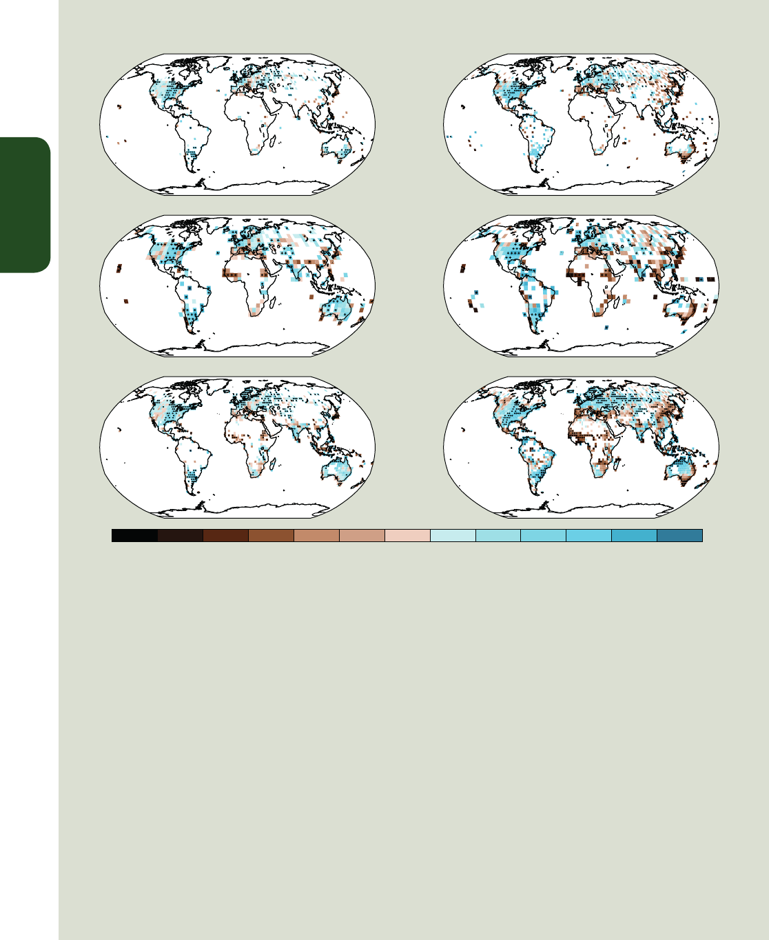
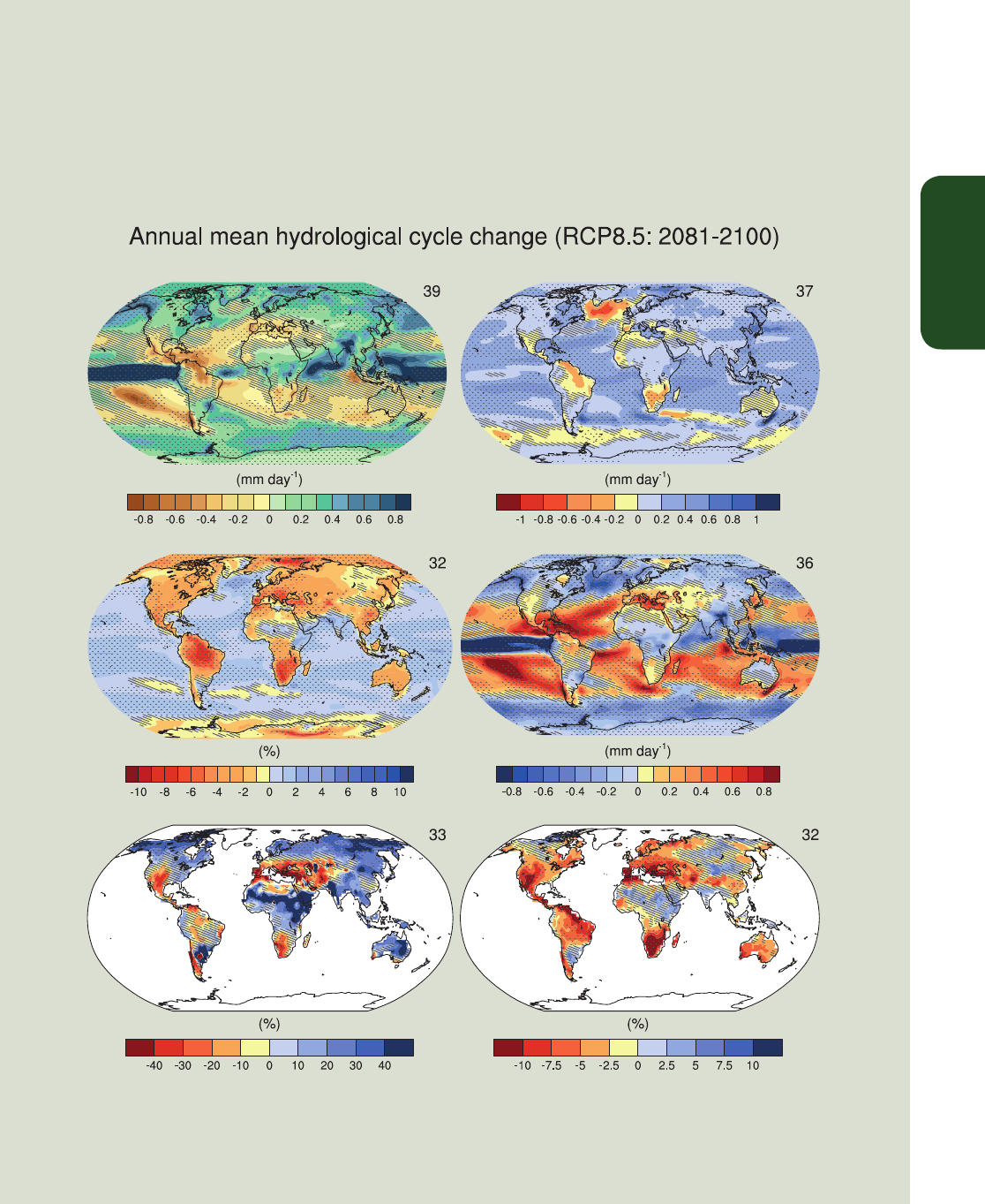
TFE.1, Figure 3 | Annual mean changes in precipitation (P), evaporation (E), relative humidity, E – P, runoff and soil moisture for 2081–2100 relative to 1986–2005
under the Representative Concentration Pathway RCP8.5 (see Box TS.6). The number of Coupled Model Intercomparison Project Phase 5 (CMIP5) models to calculate
the multi-model mean is indicated in the upper right corner of each panel. Hatching indicates regions where the multi-model mean change is less than one standard
deviation of internal variability. Stippling indicates regions where the multi-model mean change is greater than two standard deviations of internal variability and where
90% of models agree on the sign of change (see Box 12.1). {Figures 12.25–12.27}
TFE.1 (continued)
Precipitation
Relative humidity
Runoff Soil moisture
E-P
Evaporation

TS
Technical Summary
46
There is high confidence that the Antarctic ice sheet has been losing ice
during the last two decades (Figure TS.3). There is very high confidence
that these losses are mainly from the northern Antarctic Peninsula and
the Amundsen Sea sector of West Antarctica and high confidence that
they result from the acceleration of outlet glaciers. The average rate
of ice loss from Antarctica likely increased from 30 [–37 to 97] Gt yr
–1
(sea level equivalent, 0.08 [–0.10 to 0.27] mm yr
–1
) over the period
1992–2001, to 147 [72 to 221] Gt yr
–1
over the period 2002–2011
(0.40 [0.20 to 0.61] mm yr
–1
). {4.4.2, 4.4.3}
There is high confidence that in parts of Antarctica floating ice shelves
are undergoing substantial changes. There is medium confidence that
ice shelves are thinning in the Amundsen Sea region of West Antarctica,
and low confidence that this is due to high ocean heat flux. There
is high confidence that ice shelves around the Antarctic Peninsula
continue a long-term trend of retreat and partial collapse that began
decades ago. {4.4.2, 4.4.5}
TS.2.5.5 Snow Cover, Freshwater Ice and Frozen Ground
There is very high confidence that snow cover extent has decreased in
the NH, especially in spring (Figure TS.1). Satellite records indicate that
over the period 1967–2012, snow cover extent very likely decreased;
the largest change, –53% [–40 to –66%], occurred in June. No month
had statistically significant increases. Over the longer period, 1922–
2012, data are available only for March and April, but these show very
likely a 7% [4.5 to 9.5%] decline and a negative correlation (–0.76)
with March to April 40°N to 60°N land temperature. In the Southern
Hemisphere (SH), evidence is too limited to conclude whether changes
have occurred. {4.5.2, 4.5.3}
Permafrost temperatures have increased in most regions around the
world since the early 1980s (high confidence). These increases were
in response to increased air temperature and to changes in the timing
and thickness of snow cover (high confidence). The temperature
increase for colder permafrost was generally greater than for warmer
permafrost (high confidence). {4.7.2; Table 4.8}
TS.2.6 Changes in Sea Level
The primary contributions to changes in the volume of water in the
ocean are the expansion of the ocean water as it warms and the trans-
fer to the ocean of water currently stored on land, particularly from
glaciers and ice sheets. Water impoundment in reservoirs and ground
water depletion (and its subsequent runoff to the ocean) also affect
sea level. Change in sea level relative to the land (relative sea level)
can be significantly different from the global mean sea level (GMSL)
change because of changes in the distribution of water in the ocean,
vertical movement of the land and changes in the Earth’s gravitational
field. For an overview on the scientific understanding and uncertain-
ties associated with recent (and projected) sea level change see TFE.2.
{3.7.3, 13.1}
During warm intervals of the mid Pliocene (3.3 to 3.0 Ma), when
there is medium confidence that GMSTs were 1.9°C to 3.6°C warmer
than for pre-industrial climate and carbon dioxide (CO
2
) levels were
between 350 and 450 ppm, there is high confidence that GMSL was
above present, implying reduced volume of polar ice sheets. The best
estimates from various methods imply with high confidence that sea
level has not exceeded +20 m during the warmest periods of the
Pliocene, due to deglaciation of the Greenland and West Antarctic ice
sheets and areas of the East Antarctic ice sheet. {5.6.1, 13.2}
There is very high confidence that maximum GMSL during the last inter-
glacial period (129 to 116 ka) was, for several thousand years, at least
5 m higher than present and high confidence that it did not exceed 10
m above present, implying substantial contributions from the Green-
land and Antarctic ice sheets. This change in sea level occurred in the
context of different orbital forcing and with high-latitude surface tem-
perature, averaged over several thousand years, at least 2°C warmer
than present (high confidence). Based on ice sheet model simulations
consistent with elevation changes derived from a new Greenland ice
core, the Greenland ice sheet very likely contributed between 1.4 m
and 4.3 m sea level equivalent, implying with medium confidence a
contribution from the Antarctic ice sheet to the GMSL during the Last
Interglacial Period. {5.3.4, 5.6.2, 13.2.1}
Proxy and instrumental sea level data indicate a transition in the late
19th to the early 20th century from relatively low mean rates of rise
over the previous two millennia to higher rates of rise (high confi-
dence) {3.7, 3.7.4, 5.6.3, 13.2}
GMSL has risen by 0.19 [0.17 to 0.21] m, estimated from a linear trend
over the period 1901–2010, based on tide gauge records and addition-
ally on satellite data since 1993. It is very likely that the mean rate of
sea level rise was 1.7 [1.5 to 1.9] mm yr
–1
between 1901 and 2010.
Between 1993 and 2010, the rate was very likely higher at 3.2 [2.8
to 3.6] mm yr
–1
; similarly high rates likely occurred between 1920 and
1950. The rate of GMSL rise has likely increased since the early 1900s,
with estimates ranging from 0.000 [–0.002 to 0.002] to 0.013 [–0.007
to 0.019] mm yr
–2
. {3.7, 5.6.3, 13.2}
TS.2.7 Changes in Extremes
TS.2.7.1 Atmosphere
Recent analyses of extreme events generally support the AR4 and SREX
conclusions (see TFE.9 and in particular TFE.9, Table 1, for a synthesis).
It is very likely that the number of cold days and nights has decreased
and the number of warm days and nights has increased on the global
scale between 1951 and 2010. Globally, there is medium confidence
that the length and frequency of warm spells, including heat waves,
has increased since the middle of the 20th century, mostly owing to
lack of data or studies in Africa and South America. However, it is likely
that heat wave frequency has increased over this period in large parts
of Europe, Asia and Australia. {2.6.1; Tables 2.12, 2.13}
It is likely that since about 1950 the number of heavy precipitation
events over land has increased in more regions than it has decreased.
Confidence is highest for North America and Europe where there have
been likely increases in either the frequency or intensity of heavy pre-
cipitation with some seasonal and regional variations. It is very likely
that there have been trends towards heavier precipitation events in
central North America. {2.6.2; Table 2.13}

TS
Technical Summary
47
Thematic Focus Elements
TFE.2 | Sea Level Change: Scientific Understanding and Uncertainties
After the Last Glacial Maximum, global mean sea levels (GMSLs) reached close to present-day values several thou-
sand years ago. Since then, it is virtually certain that the rate of sea level rise has increased from low rates of sea
level change during the late Holocene (order tenths of mm yr
–1
) to 20th century rates (order mm yr
–1
, Figure TS1).
{3.7, 5.6, 13.2}
Ocean thermal expansion and glacier mass loss are the dominant contributors to GMSL rise during the 20th century
(high confidence). It is very likely that warming of the ocean has contributed 0.8 [0.5 to 1.1] mm yr
–1
of sea level
change during 1971–2010, with the majority of the contribution coming from the upper 700 m. The model mean
rate of ocean thermal expansion for 1971–2010 is close to observations. {3.7, 13.3}
Observations, combined with improved methods of analysis, indicate that the global glacier contribution (excluding
the peripheral glaciers around Greenland and Antarctica) to sea level was 0.25 to 0.99 mm yr
–1
sea level equivalent
during 1971–2010. Medium confidence in global glacier mass balance models used for projections of glacier chang-
es arises from the process-based understanding of glacier surface mass balance, the consistency of observations and
models of glacier changes, and the evidence that Atmosphere–Ocean General Circulation Model (AOGCM) climate
simulations can provide realitistic climate input. A simulation using observed climate data shows a larger rate of
glacier mass loss during the 1930s than the simulations using AOGCM input, possibly a result of an episode of warm-
ing in Greenland associated with unforced regional climate variability. {4.3, 13.3}
Observations indicate that the Greenland ice sheet has very likely experienced a net loss of mass due to both
increased surface melting and runoff, and increased ice discharge over the last two decades (Figure TS.3). Regional
climate models indicate that Greenland ice sheet surface mass balance showed no significant trend from the 1960s
to the 1980s, but melting and consequent runoff has increased since the early 1990s. This tendency is related to
pronounced regional warming, which may be attributed to a combination of anomalous regional variability in
recent years and anthropogenic climate change. High confidence in projections of future warming in Greenland
and increased surface melting is based on the qualitative agreements of models in projecting amplified warming at
high northern latitudes for well-understood physical reasons. {4.4, 13.3}
There is high confidence that the Antarctic ice sheet is in a state of net mass loss and its contribution to sea level
is also likely to have increased over the last two decades. Acceleration in ice outflow has been observed since the
1990s, especially in the Amundsen Sea sector of West Antarctica. Interannual variability in accumulation is large
and as a result no significant trend is present in accumulation since 1979 in either models or observations. Surface
melting is currently negligible in Antarctica. {4.4, 13.3}
Model-based estimates of climate-related changes in water storage on land (as snow cover, surface water, soil mois-
ture and ground water) do not show significant long-term contributions to sea level change for recent decades.
However, human-induced changes (reservoir impoundment and groundwater depletion) have each contributed at
least several tenths of mm yr
–1
to sea level change. Reservoir impoundment exceeded groundwater depletion for
the majority of the 20th century but the rate of groundwater depletion has increased and now exceeds the rate of
impoundment. Their combined net contribution for the 20th century is estimated to be small. {13.3}
The observed GMSL rise for 1993–2010 is consistent with the sum of the observationally estimated contributions
(TFE.2, Figure 1e). The closure of the observational budget for recent periods within uncertainties represents a
significant advance since the IPCC Fourth Assessment Report in physical understanding of the causes of past GMSL
change, and provides an improved basis for critical evaluation of models of these contributions in order to assess
their reliability for making projections. {13.3}
The sum of modelled ocean thermal expansion and glacier contributions and the estimated change in land water
storage (which is relatively small) accounts for about 65% of the observed GMSL rise for 1901–1990, and 90% for
1971–2010 and 1993–2010 (TFE.2, Figure 1). After inclusion of small long-term contributions from ice sheets and
the possible greater mass loss from glaciers during the 1930s due to unforced climate variability, the sum of the
modelled contribution is close to the observed rise. The addition of the observed ice sheet contribution since 1993
improves the agreement further between the observed and modelled sea level rise (TFE.2, Figure 1). The evidence
now available gives a clearer account than in previous IPCC assessments of 20th century sea level change. {13.3}
(continued on next page)
TS
Technical Summary
48
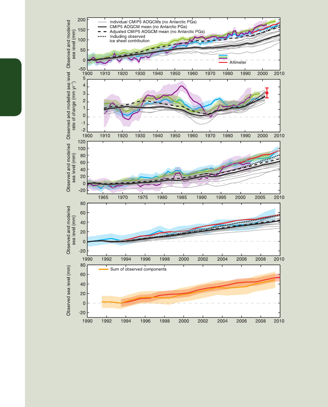
TFE.2, Figure 1 | (a) The observed and modelled sea level for 1900 to 2010. (b) The rates of sea level change for the same period, with the satellite altimeter data
shown as a red dot for the rate. (c) The observed and modelled sea level for 1961 to 2010. (d) The observed and modelled sea level for 1990 to 2010. Panel (e) com-
pares the sum of the observed contributions (orange) and the observed sea level from the satellite altimeter data (red). Estimates of GMSL from different sources are
given, with the shading indicating the uncertainty estimates (two standard deviations). The satellite altimeter data since 1993 are shown in red. The grey lines in panels
(a)-(d) are the sums of the contributions from modelled ocean thermal expansion and glaciers (excluding glaciers peripheral to the Antarctic ice sheet), plus changes
in land-water storage (see Figure 13.4). The black line is the mean of the grey lines plus a correction of thermal expansion for the omission of volcanic forcing in the
Atmosphere–Ocean General Circulation Model (AOGCM) control experiments (see Section 13.3.1). The dashed black line (adjusted model mean) is the sum of the cor-
rected model mean thermal expansion, the change in land water storage, the glacier estimate using observed (rather than modelled) climate (see Figure 13.4), and an
illustrative long-term ice-sheet contribution (of 0.1 mm yr
–1
). The dotted black line is the adjusted model mean but now including the observed ice-sheet contributions,
which begin in 1993. Because the observational ice-sheet estimates include the glaciers peripheral to the Greenland and Antarctic ice sheets (from Section 4.4), the
contribution from glaciers to the adjusted model mean excludes the peripheral glaciers (PGs) to avoid double counting. {13.3; Figure 13.7}
TFE.2 (continued)
Year
(e)
(d)
(c)
(b)
(a)
Tide gauge
TS
Technical Summary
49
TFE.2 (continued)
When calibrated appropriately, recently improved dynamical ice sheet models can reproduce the observed rapid
changes in ice sheet outflow for individual glacier systems (e.g., Pine Island Glacier in Antarctica; medium confi-
dence). However, models of ice sheet response to global warming and particularly ice sheet–ocean interactions are
incomplete and the omission of ice sheet models, especially of dynamics, from the model budget of the past means
that they have not been as critically evaluated as other contributions. {13.3, 13.4}
GMSL rise for 2081–2100 (relative to 1986–2005) for the Representative Concentration Pathways (RCPs) will likely
be in the 5 to 95% ranges derived from Coupled Model Intercomparison Project Phase 5 (CMIP5) climate projec-
tions in combination with process-based models of other contributions (medium confidence), that is, 0.26 to 0.55 m
(RCP2.6), 0.32 to 0.63 m (RCP4.5), 0.33 to 0.63 m (RCP6.0), 0.45 to 0.82 (RCP8.5) m (see Table TS.1 and Figure TS.15 for
RCP forcing). For RCP8.5 the range at 2100 is 0.52 to 0.98 m. Confidence in the projected likely ranges comes from
the consistency of process-based models with observations and physical understanding. It is assessed that there is
currently insufficient evidence to evaluate the probability of specific levels above the likely range. Based on current
understanding, only the collapse of marine-based sectors of the Antarctic ice sheet, if initiated, could cause GMSL
to rise substantially above the likely range during the 21st century. There is a lack of consensus on the probability
for such a collapse, and the potential additional contribution to GMSL rise cannot be precisely quantified, but there
is medium confidence that it would not exceed several tenths of a metre of sea level rise during the 21st century. It
is virtually certain that GMSL rise will continue beyond 2100. {13.5.1, 13.5.3}
Many semi-empirical models projections of GMSL rise are higher than process-based model projections, but there is
no consensus in the scientific community about their reliability and there is thus low confidence in their projections.
{13.5.2, 13.5.3}
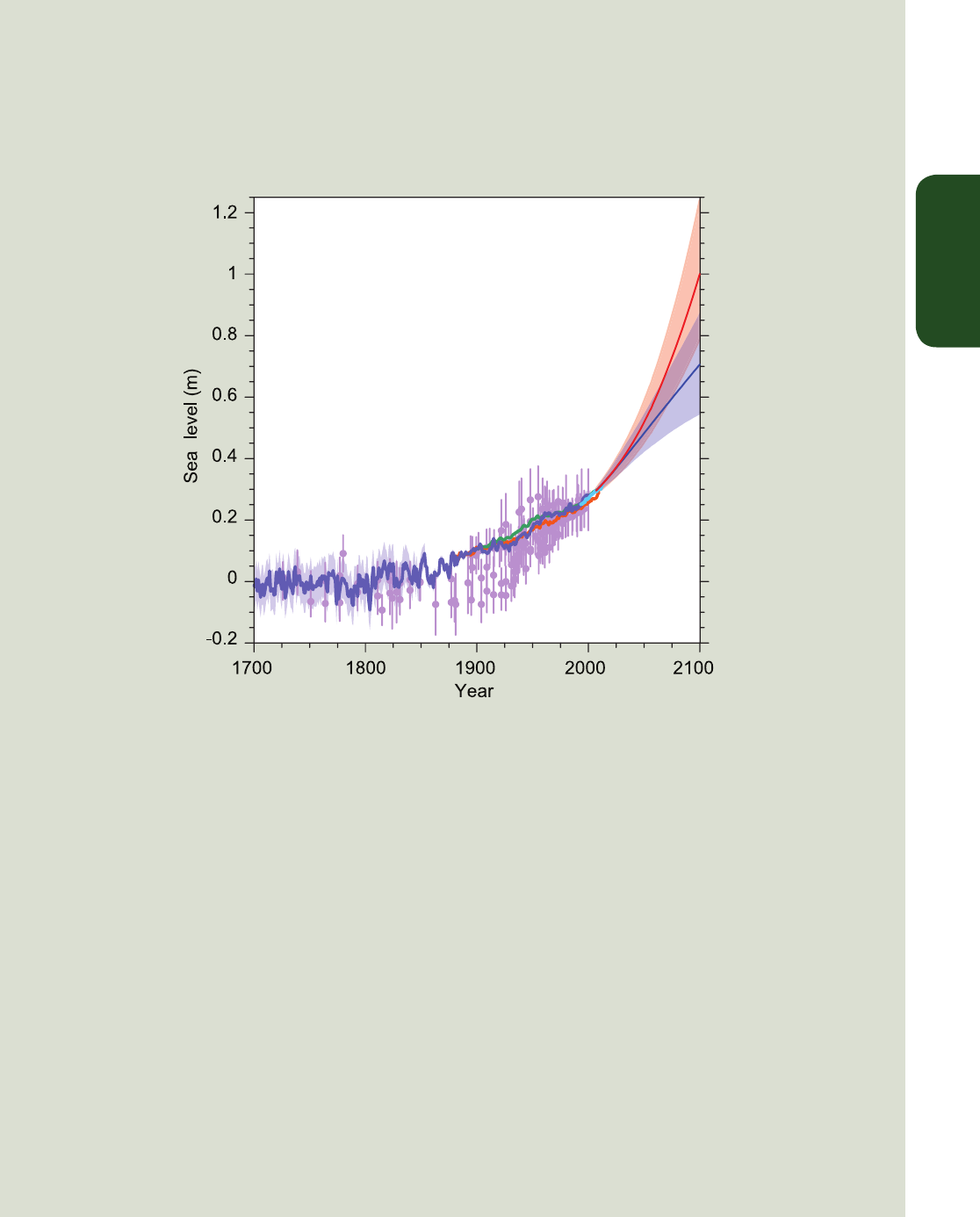
TFE.2, Figure 2 combines the paleo, tide gauge and altimeter observations of sea level rise from 1700 with the pro-
jected GMSL change to 2100. {13.5, 13.7, 13.8}
TFE.2, Figure 2 | Compilation of paleo sealevel data (purple), tide gauge data (blue, red and green), altimeter data (light blue) and central estimates and likely ranges
for projections of global mean sea level rise from the combination of CMIP5 and process-based models for RCP2.6 (blue) and RCP8.5 (red) scenarios, all relative to
pre-industrial values. {Figures 13.3, 13.11, 13.27}
TFE.2 (continued)

TS
Technical Summary
50
There is low confidence in a global-scale observed trend in drought or
dryness (lack of rainfall), owing to lack of direct observations, depen-
dencies of inferred trends on the index choice and geographical incon-
sistencies in the trends. However, this masks important regional chang-
es and, for example, the frequency and intensity of drought have likely
increased in the Mediterranean and West Africa and likely decreased
in central North America and northwest Australia since 1950. {2.6.2;
Table 2.13}
There is high confidence for droughts during the last millennium of
greater magnitude and longer duration than those observed since the
beginning of the 20th century in many regions. There is medium confi-
dence that more megadroughts occurred in monsoon Asia and wetter
conditions prevailed in arid Central Asia and the South American mon-
soon region during the Little Ice Age (1450–1850) compared to the
Medieval Climate Anomaly (950–1250). {5.5.4, 5.5.5}
Confidence remains low for long-term (centennial) changes in tropi-
cal cyclone activity, after accounting for past changes in observing
capabilities. However, for the years since the 1970s, it is virtually cer-
tain that the frequency and intensity of storms in the North Atlantic
have increased although the reasons for this increase are debated (see
TFE.9). There is low confidence of large-scale trends in storminess over
the last century and there is still insufficient evidence to determine
whether robust trends exist in small-scale severe weather events such
as hail or thunderstorms. {2.6.2–2.6.4}
With high confidence, floods larger than recorded since the 20th cen-
tury occurred during the past five centuries in northern and central
Europe, the western Mediterranean region and eastern Asia. There
is medium confidence that in the Near East, India and central North
America, modern large floods are comparable or surpass historical
floods in magnitude and/or frequency. {5.5.5}
TS.2.7.2 Oceans
It is likely that the magnitude of extreme high sea level events has
increased since 1970 (see TFE.9, Table 1). Most of the increase in
extreme sea level can be explained by the mean sea level rise: changes
in extreme high sea levels are reduced to less than 5 mm yr
–1
at 94%
of tide gauges once the rise in mean sea level is accounted for. There
is medium confidence based on reanalysis forced model hindcasts and
ship observations that mean significant wave height has increased
since the 1950s over much of the North Atlantic north of 45°N, with
typical winter season trends of up to 20 cm per decade. {3.4.5, 3.7.5}
TS.2.8 Changes in Carbon and Other Biogeochemical
Cycles
Concentrations of the atmospheric greenhouse gases (GHGs) carbon
dioxide (CO
2
), methane (CH
4
) and nitrous oxide (N
2
O) in 2011 exceed
the range of concentrations recorded in ice cores during the past 800
kyr. Past changes in atmospheric GHG concentrations are determined
9
1 Petagram of carbon = 1 PgC = 10
15
grams of carbon = 1 Gigatonne of carbon = 1 GtC. This corresponds to 3.667 GtCO
2
.
10
ppm (parts per million) or ppb (parts per billion, 1 billion = 1000 million) is the ratio of the number of greenhouse gas molecules to the total number of molecules of dry air. For
example, 300 ppm means 300 molecules of a greenhouse gas per million molecules of dry air.
with very high confidence from polar ice cores. Since AR4 these records
have been extended from 650 ka to 800 ka. {5.2.2}
With very high confidence, the current rates of CO
2
, CH
4
and N
2
O rise
in atmospheric concentrations and the associated increases in RF are
unprecedented with respect to the ‘highest resolution’ ice core records
of the last 22 kyr. There is medium confidence that the rate of change
of the observed GHG rise is also unprecedented compared with the
lower resolution records of the past 800 kyr. {2.2.1, 5.2.2}
In several periods characterized by high atmospheric CO
2
concentra-
tions, there is medium confidence that global mean temperature was
significantly above pre-industrial level. During the mid-Pliocene (3.3
to 3.0 Ma), atmospheric CO
2
concentration between 350 ppm and
450 ppm (medium confidence) occurred when GMST was 1.9°C to
3.6°C warmer (medium confidence) than for pre-industrial climate.
During the Early Eocene (52 to 48 Ma), atmospheric CO
2
concentra-
tion exceeded about 1000 ppm when GMST was 9°C to 14°C higher
(medium confidence) than for pre-industrial conditions. {5.3.1}
TS.2.8.1 Carbon Dioxide
Between 1750 and 2011, CO
2
emissions from fossil fuel combustion
and cement production are estimated from energy and fuel use sta-
tistics to have released 375 [345 to 405] PgC
9
. In 2002–2011, average
fossil fuel and cement manufacturing emissions were 8.3 [7.6 to 9.0]
PgC yr
–1
(high confidence), with an average growth rate of 3.2% yr
–1
(Figure TS.4). This rate of increase of fossil fuel emissions is higher than
during the 1990s (1.0% yr
–1
). In 2011, fossil fuel emissions were 9.5
[8.7 to 10.3] PgC. {2.2.1, 6.3.1; Table 6.1}
Between 1750 and 2011, land use change (mainly deforestation),
derived from land cover data and modelling, is estimated to have
released 180 [100 to 260] PgC. Land use change emissions between
2002 and 2011 are dominated by tropical deforestation, and are esti-
mated at 0.9 [0.1 to 1.7] PgC yr
–1
(medium confidence), with possibly a
small decrease from the 1990s due to lower reported forest loss during
this decade. This estimate includes gross deforestation emissions of
around 3 PgC yr
–1
compensated by around 2 PgC yr
–1
of forest regrowth
in some regions, mainly abandoned agricultural land. {6.3.2; Table 6.2}
Of the 555 [470 to 640] PgC released to the atmosphere from fossil
fuel and land use emissions from 1750 to 2011, 240 [230 to 250] PgC
accumulated in the atmosphere, as estimated with very high accuracy
from the observed increase of atmospheric CO
2
concentration from
278 [273 to 283] ppm
10
in 1750 to 390.5 [390.4 to 390.6] ppm in
2011. The amount of CO
2
in the atmosphere grew by 4.0 [3.8 to 4.2]
PgC yr
–1
in the first decade of the 21st century. The distribution of
observed atmospheric CO
2
increases with latitude clearly shows that
the increases are driven by anthropogenic emissions that occur primar-
ily in the industrialized countries north of the equator. Based on annual
average concentrations, stations in the NH show slightly higher con-
centrations than stations in the SH. An independent line of evidence
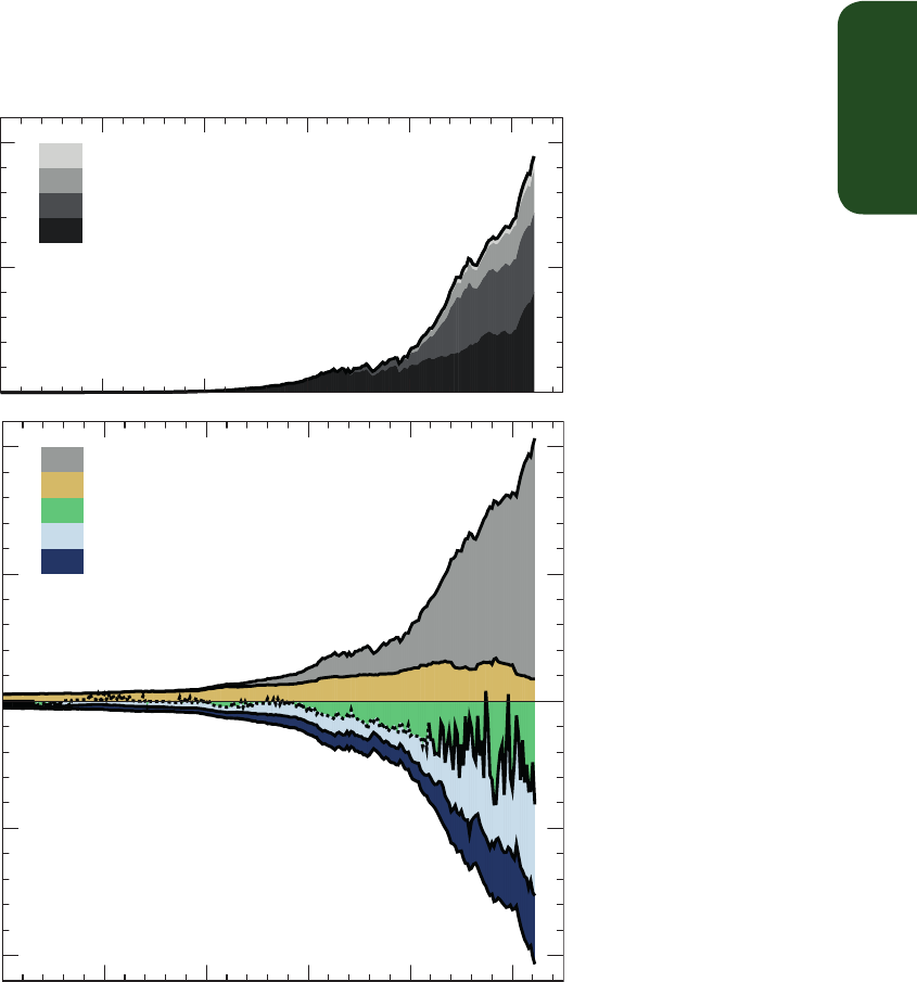
TS
Technical Summary
51
Figure TS.4 | Annual anthropogenic CO
2
emissions and their partitioning among the atmosphere, land and ocean (PgC yr
–1
) from 1750 to 2011. (Top) Fossil fuel and cement
CO
2
emissions by category, estimated by the Carbon Dioxide Information Analysis Center (CDIAC). (Bottom) Fossil fuel and cement CO
2
emissions as above. CO
2
emissions from
net land use change, mainly deforestation, are based on land cover change data (see Table 6.2). The atmospheric CO
2
growth rate prior to 1959 is based on a spline fit to ice core
observations and a synthesis of atmospheric measurements from 1959. The fit to ice core observations does not capture the large interannual variability in atmospheric CO
2
and
is represented with a dashed line. The ocean CO
2
sink is from a combination of models and observations. The residual land sink (term in green in the figure) is computed from the
residual of the other terms. The emissions and their partitioning include only the fluxes that have changed since 1750, and not the natural CO
2
fluxes (e.g., atmospheric CO
2
uptake
from weathering, outgassing of CO
2
from lakes and rivers and outgassing of CO
2
by the ocean from carbon delivered by rivers; see Figure 6.1) between the atmosphere, land and
ocean reservoirs that existed before that time and still exist today. The uncertainties in the various terms are discussed in Chapter 6 and reported in Table 6.1 for decadal mean
values. {Figure 6.8}
cement
gas
oil
coal
fossil fuel and cement from energy statistics
land use change from data and models
residual land sink
measured atmospheric growth rate
ocean sink from data and models
1750 1800 1850 1900 1950 2000
10
5
5
10
0
5
10
0
1750 1800 1850 1900 1950 2000
emissions
partitioning
Annual anthropogenic CO
2
emissions
and partitioning (PgC yr
–1
)
Fossil fuel and cement
CO
2
emissions (PgC yr
–1
)
Year
for the anthropogenic origin of the observed atmospheric CO
2
increase
comes from the observed consistent decrease in atmospheric oxygen
(O
2
) content and a decrease in the stable isotopic ratio of CO
2
(
13
C/
12
C)
in the atmosphere (Figure TS.5). {2.2.1, 6.1.3}
The remaining amount of carbon released by fossil fuel and land
use emissions has been re-absorbed by the ocean and terrestrial
ecosystems. Based on high agreement between independent esti-
mates using different methods and data sets (e.g., oceanic carbon,
oxygen and transient tracer data), it is very likely that the global ocean
inventory of anthropogenic carbon increased from 1994 to 2010. In
2011, it is estimated to be 155 [125 to 185] PgC. The annual global
oceanic uptake rates calculated from independent data sets (from
changes in the oceanic inventory of anthropogenic carbon, from mea-
surements of the atmospheric oxygen to nitrogen ratio (O
2
/N
2
) or from
CO
2
partial pressure (pCO
2
) data) and for different time periods agree
with each other within their uncertainties, and very likely are in the
range of 1.0 to 3.2 PgC yr
–1
. Regional observations of the storage
rate of anthropogenic carbon in the ocean are in broad agreement
with the expected rate resulting from the increase in atmospheric CO
2
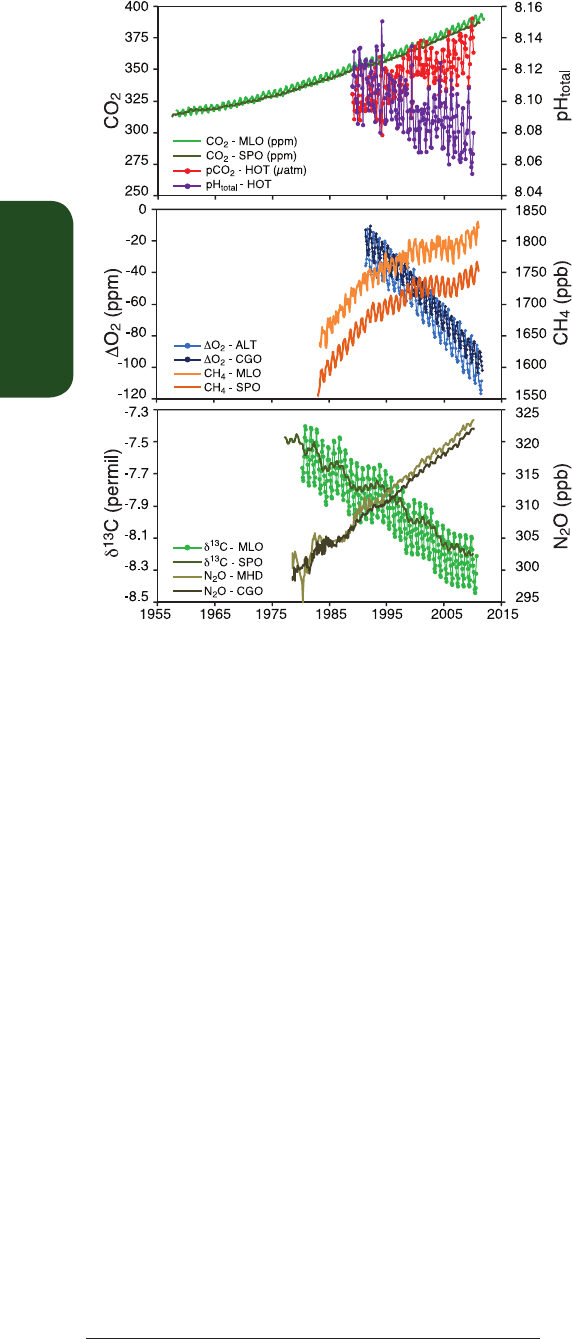
TS
Technical Summary
52
concentrations, but with significant spatial and temporal variations.
{3.8.1, 6.3}
Natural terrestrial ecosystems (those not affected by land use change)
are estimated by difference from changes in other reservoirs to have
accumulated 160 [70 to 250] PgC between 1750 and 2011. The gain
of carbon by natural terrestrial ecosystems is estimated to take place
mainly through the uptake of CO
2
by enhanced photosynthesis at
higher CO
2
levels and nitrogen deposition and longer growing seasons
in mid and high latitudes. Natural carbon sinks vary regionally owing
to physical, biological and chemical processes acting on different time
scales. An excess of atmospheric CO
2
absorbed by land ecosystems
gets stored as organic matter in diverse carbon pools, from short-lived
(leaves, fine roots) to long-lived (stems, soil carbon). {6.3; Table 6.1}
TS.2.8.2 Carbon and Ocean Acidification
Oceanic uptake of anthropogenic CO
2
results in gradual acidification of
the ocean. The pH
11
of ocean surface water has decreased by 0.1 since
the beginning of the industrial era (high confidence), corresponding to
a 26% increase in hydrogen ion concentration. The observed pH trends
range between –0.0014 and –0.0024 per year in surface waters. In
the ocean interior, natural physical and biological processes, as well as
uptake of anthropogenic CO
2
, can cause changes in pH over decadal
and longer time scales. {3.8.2; Box 3.2; Table 3.2; FAQ 3.3}
TS.2.8.3 Methane
The concentration of CH
4
has increased by a factor of 2.5 since pre-
industrial times, from 722 [697 to 747] ppb in 1750 to 1803 [1799 to
1807] ppb in 2011 (Figure TS.5). There is very high confidence that the
atmospheric CH
4
increase during the Industrial Era is caused by anthro-
pogenic activities. The massive increase in the number of ruminants,
the emissions from fossil fuel extraction and use, the expansion of
rice paddy agriculture and the emissions from landfills and waste are
the dominant anthropogenic CH
4
sources. Anthropogenic emissions
account for 50 to 65% of total emissions. By including natural geologi-
cal CH
4
emissions that were not accounted for in previous budgets, the
fossil component of the total CH
4
emissions (i.e., anthropogenic emis-
sions related to leaks in the fossil fuel industry and natural geological
leaks) is now estimated to amount to about 30% of the total CH
4
emis-
sions (medium confidence). {2.2.1, 6.1, 6.3.3}
In recent decades, CH
4
growth in the atmosphere has been variable. CH
4
concentrations were relatively stable for about a decade in the 1990s,
but then started growing again starting in 2007. The exact drivers of
this renewed growth are still debated. Climate-driven fluctuations of
CH
4
emissions from natural wetlands (177 to 284 ×10
12
g (CH
4
) yr
–1
for
2000–2009 based on bottom-up estimates) are the main drivers of the
global interannual variability of CH
4
emissions (high confidence), with
a smaller contribution from biomass burning emissions during high fire
years {2.2.1, 6.3.3; Table 6.8}.
TS.2.8.4 Nitrous Oxide
Since pre-industrial times, the concentration of N
2
O in the atmosphere
has increased by a factor of 1.2 (Figure TS.5). Changes in the nitro-
gen cycle, in addition to interactions with CO
2
sources and sinks, affect
emissions of N
2
O both on land and from the ocean. {2.2.1, 6.4.6}
TS.2.8.5 Oceanic Oxygen
High agreement among analyses provides medium confidence that
oxygen concentrations have decreased in the open ocean thermocline
in many ocean regions since the 1960s. The general decline is con-
sistent with the expectation that warming-induced stratification leads
to a decrease in the supply of oxygen to the thermocline from near
surface waters, that warmer waters can hold less oxygen and that
changes in wind-driven circulation affect oxygen concentrations. It is
likely that the tropical oxygen minimum zones have expanded in recent
decades. {3.8.3}
Figure TS.5 | Atmospheric concentration of CO
2
, oxygen,
13
C/
12
C stable isotope ratio
in CO
2
, as well as CH
4
and N
2
O atmospheric concentrations and oceanic surface obser-
vations of CO
2
partial pressure (pCO
2
) and pH, recorded at representative time series
stations in the Northern and the Southern Hemispheres. MLO: Mauna Loa Observatory,
Hawaii; SPO: South Pole; HOT: Hawaii Ocean Time-Series station; MHD: Mace Head,
Ireland; CGO: Cape Grim, Tasmania; ALT: Alert, Northwest Territories, Canada. Further
detail regarding the related Figure SPM.4 is given in the TS Supplementary Material.
{Figures 3.18, 6.3; FAQ 3.3, Figure 1}
11
pH is a measure of acidity: a decrease in pH value means an increase in acidity, that is, acidification.

TS
Technical Summary
53
TS.3 Drivers of Climate Change
TS.3.1 Introduction
Human activities have changed and continue to change the Earth’s
surface and atmospheric composition. Some of these changes have
a direct or indirect impact on the energy balance of the Earth and are
thus drivers of climate change. Radiative forcing (RF) is a measure of
the net change in the energy balance of the Earth system in response to
some external perturbation (see Box TS.2), with positive RF leading to
a warming and negative RF to a cooling. The RF concept is valuable for
comparing the influence on GMST of most individual agents affecting
the Earth’s radiation balance. The quantitative values provided in AR5
are consistent with those in previous IPCC reports, though there have
been some important revisions (Figure TS.6). Effective radiative forc-
ing (ERF) is now used to quantify the impact of some forcing agents
that involve rapid adjustments of components of the atmosphere and
surface that are assumed constant in the RF concept (see Box TS.2).
RF and ERF are estimated from the change between 1750 and 2011,
referred to as ‘Industrial Era’, if other time periods are not explicitly
stated. Uncertainties are given associated with the best estimates of
RF and ERF, with values representing the 5 to 95% (90%) confidence
range. {8.1, 7.1}
In addition to the global mean RF or ERF, the spatial distribution and
temporal evolution of forcing, as well as climate feedbacks, play a
role in determining the eventual impact of various drivers on climate.
Land surface changes may also impact the local and regional climate
through processes that are not radiative in nature. {8.1, 8.3.5, 8.6}
TS.3.2 Radiative Forcing from Greenhouse Gases
Human activity leads to change in the atmospheric composition either
directly (via emissions of gases or particles) or indirectly (via atmo-
spheric chemistry). Anthropogenic emissions have driven the changes
Box TS.2 | Radiative Forcing and Effective Radiative Forcing
RF and ERF are used to quantify the change in the Earth’s energy balance that occurs as a result of an externally imposed change. They
are expressed in watts per square metre (W m
–2
). RF is defined in AR5, as in previous IPCC assessments, as the change in net downward
flux (shortwave + longwave) at the tropopause after allowing for stratospheric temperatures to readjust to radiative equilibrium, while
holding other state variables such as tropospheric temperatures, water vapour and cloud cover fixed at the unperturbed values (see
Glossary). {8.1.1}
Although the RF concept has proved very valuable, improved understanding has shown that including rapid adjustments of the Earth’s
surface and troposphere can provide a better metric for quantifying the climate response. These rapid adjustments occur over a variety
of time scales, but are relatively distinct from responses to GMST change. Aerosols in particular impact the atmosphere temperature
profile and cloud properties on a time scale much shorter than adjustments of the ocean (even the upper layer) to forcings. The ERF
concept defined in AR5 allows rapid adjustments to perturbations, for all variables except for GMST or ocean temperature and sea ice
cover. The ERF and RF values are significantly different for the anthropogenic aerosols, owing to their influence on clouds and on snow
or ice cover. For other components that drive the Earth’s energy balance, such as GHGs, ERF and RF are fairly similar, and RF may have
comparable utility given that it requires fewer computational resources to calculate and is not affected by meteorological variability
and hence can better isolate small forcings. In cases where RF and ERF differ substantially, ERF has been shown to be a better indicator
of the GMST response and is therefore emphasized in AR5. {7.1, 8.1; Box 8.1}
in well-mixed greenhouse gas (WMGHG) concentrations during the
Industrial Era (see Section TS.2.8 and TFE.7). As historical WMGHG
concentrations since the pre-industrial are well known based on direct
measurements and ice core records, and WMGHG radiative proper-
ties are also well known, the computation of RF due to concentra-
tion changes provides tightly constrained values (Figure TS.6). There
has not been significant change in our understanding of WMGHG
radiative impact, so that the changes in RF estimates relative to AR4
are due essentially to concentration increases. The best estimate for
WMGHG ERF is the same as RF, but the uncertainty range is twice as
large due to the poorly constrained cloud responses. Owing to high-
quality observations, it is certain that increasing atmospheric burdens
of most WMGHGs, especially CO
2
, resulted in a further increase in their
RF from 2005 to 2011. Based on concentration changes, the RF of all
WMGHGs in 2011 is 2.83 [2.54 to 3.12] W m
–2
(very high confidence).
This is an increase since AR4 of 0.20 [0.18 to 0.22] W m
–2
, with nearly
all of the increase due to the increase in the abundance of CO
2
since
2005. The Industrial Era RF for CO
2
alone is 1.82 [1.63 to 2.01] W m
–2
.
Over the last 15 years, CO
2
has been the dominant contributor to the
increase in RF from the WMGHGs, with RF of CO
2
having an average
growth rate slightly less than 0.3 W m
–2
per decade. The uncertainty in
the WMGHG RF is due in part to its radiative properties but mostly to
the full accounting of atmospheric radiative transfer including clouds.
{2.2.1, 5.2, 6.3, 8.3, 8.3.2; Table 6.1}
After a decade of near stability, the recent increase of CH
4
concentra-
tion led to an enhanced RF compared to AR4 by 2% to 0.48 [0.43 to
0.53] W m
–2
. It is very likely that the RF from CH
4
is now larger than that
of all halocarbons combined. {2.2.1, 8.3.2}
Atmospheric N
2
O has increased by 6% since AR4, causing an RF of 0.17
[0.14 to 0.20] W m
–2
. N
2
O concentrations continue to rise while those
of dichlorodifluoromethane (CF
2
Cl
2
, CFC-12), the third largest WMGHG
contributor to RF for several decades, are decreasing due to phase-
out of emissions of this chemical under the Montreal Protocol. Since
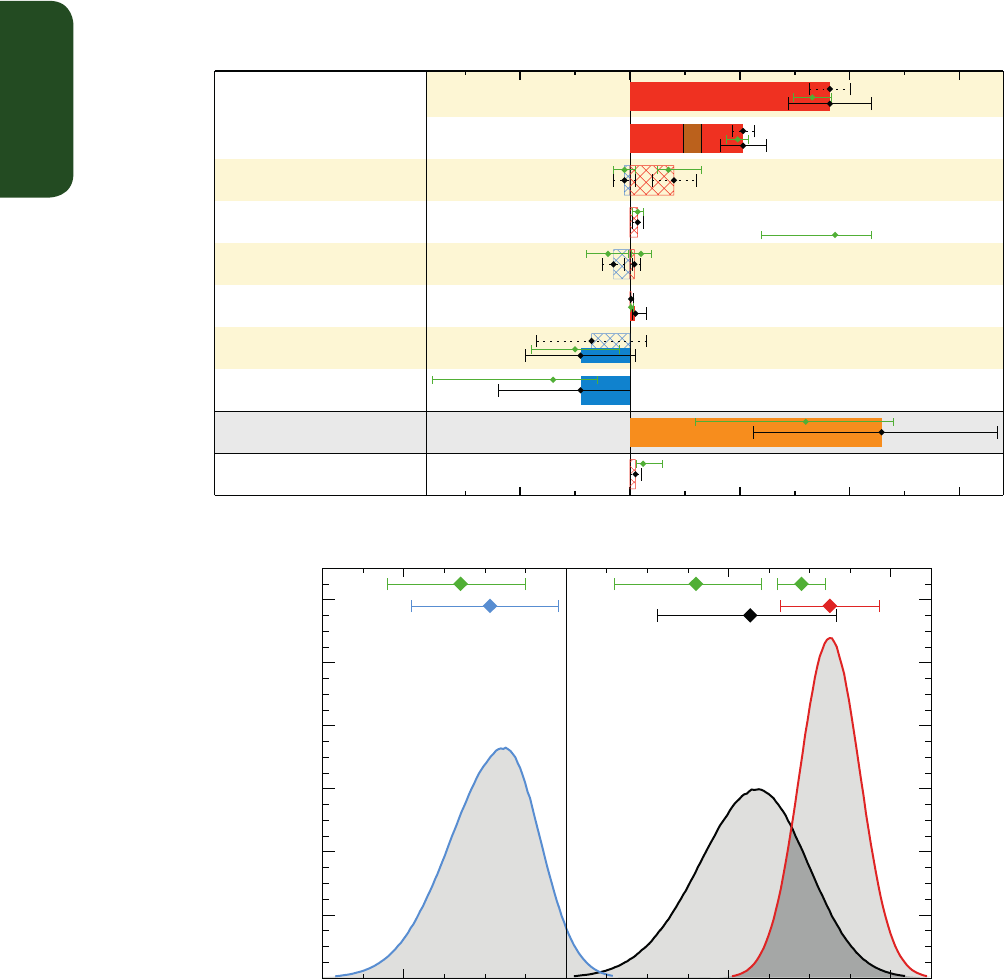
TS
Technical Summary
54
Natural Anthropogenic
Well Mixed
Greenhouse Gases
Forcing agent
Radiative forcing of climate between 1750 and 2011
-1 0 1 2 3
CO
2
Other WMGHG CH
4
N
2
O
Halocarbons
TroposphericStratospheric Ozone
Stratospheric water
vapour from CH
4
Land Use
Black carbon
on snow
Surface Albedo
Contrail induced cirrus
Contrails
Aerosol-Radiation Interac.
Aerosol-Cloud Interac.
Total anthropogenic
Solar irradiance
AR4 estimates
Medium
Low
Medium
High
Low
Medium
High/Low
Medium
High
Very High
Very High
Level
Confidence
Radiative Forcing (W m
-2
)
Greenhouse
gases
Total
anthropogenic
Aerosols
AR4 RF
-2 0 2 4
Effective radiative forcing (W m
-2
)
0.0
0.2
0.4
0.6
0.8
1.0
1.2
Probability density function
Figure TS.6 | Radiative forcing (RF) and Effective radiative forcing (ERF) of climate change during the Industrial Era. (Top) Forcing by concentration change between 1750 and
2011 with associated uncertainty range (solid bars are ERF, hatched bars are RF, green diamonds and associated uncertainties are for RF assessed in AR4). (Bottom) Probability
density functions (PDFs) for the ERF, for the aerosol, greenhouse gas (GHG) and total. The green lines show the AR4 RF 90% confidence intervals and can be compared with the red,
blue and black lines which show the AR5 ERF 90% confidence intervals (although RF and ERF differ, especially for aerosols). The ERF from surface albedo changes and combined
contrails and contrail-induced cirrus is included in the total anthropogenic forcing, but not shown as a separate PDF. For some forcing mechanisms (ozone, land use, solar) the RF is
assumed to be representative of the ERF but an additional uncertainty of 17% is added in quadrature to the RF uncertainty. {Figures 8.15, 8.16}
AR4, N
2
O has overtaken CFC-12 to become the third largest WMGHG
contributor to RF. The RF from halocarbons is very similar to the value
in AR4, with a reduced RF from CFCs but increases in many of their
replacements. Four of the halocarbons (trichlorofluoromethane (CFCl
3
,
CFC-11), CFC-12, trichlorotrifluoroethane (CF
2
ClCFCl
2
, CFC-113) and
chlorodifluoromethane (CHF
2
Cl, HCFC-22) account for 85% of the total
halocarbon RF. The former three compounds have declining RF over
the last 5 years but are more than compensated for by the increased
RF from HCFC-22. There is high confidence that the growth rate in RF
from all WMGHG is weaker over the last decade than in the 1970s and
1980s owing to a slower increase in the non-CO
2
RF. {2.2.1, 8.3.2}
The short-lived GHGs ozone (O
3
) and stratospheric water vapour also
contribute to anthropogenic forcing. Observations indicate that O
3
likely increased at many undisturbed (background) locations through
the 1990s. These increases have continued mainly over Asia (though

TS
Technical Summary
55
observations cover a limited area) and flattened over Europe during
the last decade. The total RF due to changes in O
3
is 0.35 [0.15 to 0.55]
W m
–2
(high confidence), with RF due to tropospheric O
3
of 0.40 [0.20
to 0.60] W m
–2
(high confidence) and due to stratospheric O
3
of –0.05
[–0.15 to +0.05] W m
–2
(high confidence). O
3
is not emitted directly
into the atmosphere; instead it is formed by photochemical reactions.
In the troposphere these reactions involve precursor compounds that
are emitted into the atmosphere from a variety of natural and anthro-
pogenic sources. Tropospheric O
3
RF is largely attributed to increases
in emissions of CH
4
, carbon monoxide, volatile organics and nitrogen
oxides, while stratospheric RF results primarily from O
3
depletion by
anthropogenic halocarbons. However, there is now strong evidence
for substantial links between the changes in tropospheric and strato-
spheric O
3
and a total O
3
RF of 0.50 [0.30 to 0.70] W m
–2
is attributed
to tropospheric O
3
precursor emissions and –0.15 [–0.30 to 0.00] W
m
–2
to O
3
depletion by halocarbons. There is strong evidence that tro-
pospheric O
3
also has a detrimental impact on vegetation physiology,
and therefore on its CO
2
uptake. This reduced uptake leads to an indi-
rect increase in the atmospheric CO
2
concentration. Thus a fraction of
the CO
2
RF should be attributed to ozone or its precursors rather than
direct emission of CO
2
, but there is a low confidence on the quantita-
tive estimates. RF for stratospheric water vapour produced from CH
4
oxidation is 0.07 [0.02 to 0.12] W m
–2
. Other changes in stratospheric
water vapour, and all changes in water vapour in the troposphere, are
regarded as a feedback rather than a forcing. {2.2.2, 8.1–8.3; FAQ 8.1}
TS.3.3 Radiative Forcing from Anthropogenic Aerosols
Anthropogenic aerosols are responsible for an RF of climate through
multiple processes which can be grouped into two types: aerosol–radi-
ation interactions (ari) and aerosol–cloud interactions (aci). There has
been progress since AR4 on observing and modelling climate-relevant
aerosol properties (including their size distribution, hygroscopicity,
chemical composition, mixing state, optical and cloud nucleation prop-
erties) and their atmospheric distribution. Nevertheless, substantial
uncertainties remain in assessments of long-term trends of global
aerosol optical depth and other global properties of aerosols due to
difficulties in measurement and lack of observations of some relevant
parameters, high spatial and temporal variability and the relatively
short observational records that exist. The anthropogenic RFari is given
a best estimate of –0.35 [–0.85 to +0.15] W m
–2
(high confidence)
using evidence from aerosol models and some constraints from obser-
vations. The RFari is caused by multiple aerosol types (see Section
TS3.6). The rapid adjustment to RFari leads to further negative forcing,
in particular through cloud adjustments, and is attributable primarily
to black carbon. As a consequence, the ERFari is more negative than
the RFari (low confidence) and given a best estimate of –0.45 [–0.95 to
+0.05] W m
–2
. The assessment for RFari is less negative than reported
in AR4 because of a re-evaluation of aerosol absorption. The uncer-
tainty estimate is wider but more robust. {2.2.3, 7.3, 7.5.2}
Improved understanding of aerosol–cloud interactions has led to a
reduction in the magnitude of many global aerosol–cloud forcings esti-
mates. The total ERF due to aerosols (ERFari+aci, excluding the effect
of absorbing aerosol on snow and ice) is assessed to be –0.9 [–1.9
to –0.1] W m
–2
(medium confidence). This estimate encompasses all
rapid adjustments, including changes to the cloud lifetime and aerosol
microphysical effects on mixed-phase, ice and convective clouds. This
range was obtained by giving equal weight to satellite-based studies
and estimates from climate models. It is consistent with multiple lines
of evidence suggesting less negative estimates for aerosol–cloud inter-
actions than those discussed in AR4. {7.4, 7.5, 8.5}
The RF from black carbon (BC) on snow and ice is assessed to be 0.04
[0.02 to 0.09] W m
–2
(low confidence). Unlike in the previous IPCC
assessment, this estimate includes the effects on sea ice, accounts for
more physical processes and incorporates evidence from both models
and observations. This RF causes a two to four times larger GMST
change per unit forcing than CO
2
primarily because all of the forc-
ing energy is deposited directly into the cryosphere, whose evolution
drives a positive albedo feedback on climate. This effect thus can rep-
resent a significant forcing mechanism in the Arctic and other snow- or
ice-covered regions. {7.3, 7.5.2, 8.3.4, 8.5}
Despite the large uncertainty ranges on aerosol forcing, there is a high
confidence that aerosols have offset a substantial portion of GHG
forcing. Aerosol–cloud interactions can influence the character of indi-
vidual storms, but evidence for a systematic aerosol effect on storm or
precipitation intensity is more limited and ambiguous. {7.4, 7.6, 8.5}
TS.3.4 Radiative Forcing from Land Surface Changes
and Contrails
There is robust evidence that anthropogenic land use changes such as
deforestation have increased the land surface albedo, which leads to
an RF of –0.15 [–0.25 to –0.05] W m
–2
. There is still a large spread of
quantitative estimates owing to different assumptions for the albedo of
natural and managed surfaces (e.g., croplands, pastures). In addition,
the time evolution of the land use change, and in particular how much
was already completed in the reference year 1750, are still debated.
Furthermore, land use change causes other modifications that are not
radiative but impact the surface temperature, including modifications
in the surface roughness, latent heat flux, river runoff and irrigation.
These are more uncertain and they are difficult to quantify, but they
tend to offset the impact of albedo changes at the global scale. As a
consequence, there is low agreement on the sign of the net change
in global mean temperature as a result of land use change. Land use
change, and in particular deforestation, also has significant impacts on
WMGHG concentrations. It contributes to the corresponding RF associ-
ated with CO
2
emissions or concentration changes. {8.3.5}
Persistent contrails from aviation contribute a positive RF of 0.01
[0.005 to 0.03] W m
–2
(medium confidence) for year 2011, and the
combined contrail and contrail-cirrus ERF from aviation is assessed to
be 0.05 [0.02 to 0.15] W m
–2
(low confidence). This forcing can be much
larger regionally but there is now medium confidence that it does not
produce observable regional effects on either the mean or diurnal
range of surface temperature. {7.2.7}
TS.3.5 Radiative Forcing from Natural Drivers of
Climate Change
Solar and volcanic forcings are the two dominant natural contributors
to global climate change during the Industrial Era. Satellite observations

TS
Technical Summary
56
of total solar irradiance (TSI) changes since 1978 show quasi-periodic
cyclical variation with a period of roughly 11 years. Longer term forc-
ing is typically estimated by comparison of solar minima (during which
variability is least). This gives an RF change of –0.04 [–0.08 to 0.00] W
m
–2
between the most recent (2008) minimum and the 1986 minimum.
There is some diversity in the estimated trends of the composites of
various satellite data, however. Secular trends of TSI before the start
of satellite observations rely on a number of indirect proxies. The best
estimate of RF from TSI changes over the industrial era is 0.05 [0.00
to 0.10] W m
–2
(medium confidence), which includes greater RF up to
around 1980 and then a small downward trend. This RF estimate is
substantially smaller than the AR4 estimate due to the addition of the
latest solar cycle and inconsistencies in how solar RF was estimated in
earlier IPCC assessments. The recent solar minimum appears to have
been unusually low and long-lasting and several projections indicate
lower TSI for the forthcoming decades. However, current abilities to
project solar irradiance are extremely limited so that there is very low
confidence concerning future solar forcing. Nonetheless, there is a high
confidence that 21st century solar forcing will be much smaller than
the projected increased forcing due to WMGHGs. {5.2.1, 8.4.1; FAQ 5.1}
Changes in solar activity affect the cosmic ray flux impinging upon
the Earth’s atmosphere, which has been hypothesized to affect climate
through changes in cloudiness. Cosmic rays enhance aerosol nucleation
and thus may affect cloud condensation nuclei production in the free
troposphere, but the effect is too weak to have any climatic influence
during a solar cycle or over the last century (medium evidence, high
agreement). No robust association between changes in cosmic rays
and cloudiness has been identified. In the event that such an associa-
tion existed, a mechanism other than cosmic ray–induced nucleation
of new aerosol particles would be needed to explain it. {7.3, 7.4.6}
The RF of stratospheric volcanic aerosols is now well understood and
there is a large RF for a few years after major volcanic eruptions (Box
TS.5, Figure 1). Although volcanic eruptions inject both mineral par-
ticles and sulphate aerosol precursors into the atmosphere, it is the
latter, because of their small size and long lifetimes, that are respon-
sible for RF important for climate. The emissions of CO
2
from volcanic
eruptions are at least 100 times smaller than anthropogenic emissions,
and inconsequential for climate on century time scales. Large tropical
volcanic eruptions have played an important role in driving annual to
decadal scale climate change during the Industrial Era owing to their
sometimes very large negative RF. There has not been any major vol-
canic eruption since Mt Pinatubo in 1991, which caused a 1-year RF
of about –3.0 W m
–2
, but several smaller eruptions have caused an
RF averaged over the years 2008–2011 of –0.11 [–0.15 to –0.08] W
m
–2
(high confidence), twice as strong in magnitude compared to the
1999–2002 average. The smaller eruptions have led to better under-
standing of the dependence of RF on the amount of material from
high-latitude injections as well as the time of the year when they take
place. {5.2.1, 5.3.5, 8.4.2; Annex II}
TS.3.6 Synthesis of Forcings; Spatial and Temporal
Evolution
A synthesis of the Industrial Era forcing finds that among the forcing
agents, there is a very high confidence only for the WMGHG RF. Relative
to AR4, the confidence level has been elevated for seven forcing agents
owing to improved evidence and understanding. {8.5; Figure 8.14}
The time evolution of the total anthropogenic RF shows a nearly con-
tinuous increase from 1750, primarily since about 1860. The total
anthropogenic RF increase rate since 1960 has been much greater than
during earlier Industrial Era periods, driven primarily by the continuous
increase in most WMGHG concentrations. There is still low agreement
on the time evolution of the total aerosol ERF, which is the primary
factor for the uncertainty in the total anthropogenic forcing. The frac-
tional uncertainty in the total anthropogenic forcing decreases gradual-
ly after 1950 owing to the smaller offset of positive WMGHG forcing by
negative aerosol forcing. There is robust evidence and high agreement
that natural forcing is a small fraction of the WMGHG forcing. Natural
forcing changes over the last 15 years have likely offset a substantial
fraction (at least 30%) of the anthropogenic forcing increase during
this period (Box TS.3). Forcing by CO
2
is the largest single contribu-
tor to the total forcing during the Industrial Era and from 1980–2011.
Compared to the entire Industrial Era, the dominance of CO
2
forcing
is larger for the 1980–2011 change with respect to other WMGHGs,
and there is high confidence that the offset from aerosol forcing to
WMGHG forcing during this period was much smaller than over the
1950–1980 period. {8.5.2}
Forcing can also be attributed to emissions rather than to the result-
ing concentration changes (Figure TS.7). Carbon dioxide is the largest
single contributor to historical RF from either the perspective of chang-
es in the atmospheric concentration of CO
2
or the impact of changes in
net emissions of CO
2
. The relative importance of other forcing agents
can vary markedly with the perspective chosen, however. In particu-
lar, CH
4
emissions have a much larger forcing (about 1.0 W m
–2
over
the Industrial Era) than CH
4
concentration increases (about 0.5 W m
–2
)
due to several indirect effects through atmospheric chemistry. In addi-
tion, carbon monoxide emissions are virtually certain to cause a posi-
tive forcing, while emissions of reactive nitrogen oxides likely cause a
net negative forcing but uncertainties are large. Emissions of ozone-
depleting halocarbons very likely cause a net positive forcing as their
direct radiative effect is larger than the impact of the stratospheric
ozone depletion that they induce. Emissions of SO
2
, organic carbon and
ammonia cause a negative forcing, while emissions of black carbon
lead to positive forcing via aerosol–radiation interactions. Note that
mineral dust forcing may include a natural component or a climate
feedback effect. {7.3, 7.5.2, 8.5.1}
Although the WMGHGs show a spatially fairly homogeneous forcing,
other agents such as aerosols, ozone and land use changes are highly
heterogeneous spatially. RFari showed maximum negative values over
eastern North America and Europe during the early 20th century, with
large negative values extending to East and Southeast Asia, South
America and central Africa by 1980. Since then, however, the magnitude
has decreased over eastern North America and Europe due to pollution
control, and the peak negative forcing has shifted to South and East
Asia primarily as a result of economic growth and the resulting increase
in emissions in those areas. Total aerosol ERF shows similar behaviour
for locations with maximum negative forcing, but also shows substan-
tial positive forcing over some deserts and the Arctic. In contrast, the
global mean whole atmosphere ozone forcing increased throughout

TS
Technical Summary
57
the 20th century, and has peak positive amplitudes around 15°N to
30°N but negative values over Antarctica. Negative land use forcing
by albedo changes has been strongest in industrialized and biomass
burning regions. The inhomogeneous nature of these forcings can cause
them to have a substantially larger influence on the hydrologic cycle
than an equivalent global mean homogeneous forcing. {8.3.5, 8.6}
Over the 21st century, anthropogenic RF is projected to increase under
the Representative Concentration Pathways (RCPs; see Box TS.6).
Simple model estimates of the RF resulting from the RCPs, which
include WMGHG emissions spanning a broad range of possible futures,
show anthropogenic RF relative to 1750 increasing to 3.0 to 4.8 W
m
–2
in 2050, and 2.7 to 8.4 W m
–2
at 2100. In the near term, the RCPs
are quite similar to one another (and emissions of near-term climate
forcers do not span the literature range of possible futures), with RF
at 2030 ranging only from 2.9 to 3.3 W m
–2
(additional 2010 to 2030
RF of 0.7 to 1.1 W m
–2
), but they show highly diverging values for the
second half of the 21st century driven largely by CO
2
. Results based on
Figure TS.7 | Radiative forcing (RF) of climate change during the Industrial Era shown by emitted components from 1750 to 2011. The horizontal bars indicate the overall uncer-
tainty, while the vertical bars are for the individual components (vertical bar lengths proportional to the relative uncertainty, with a total length equal to the bar width for a ±50%
uncertainty). Best estimates for the totals and individual components (from left to right) of the response are given in the right column. Values are RF except for the effective radiative
forcing (ERF) due to aerosol–cloud interactions (ERFaci) and rapid adjustment associated with the RF due to aerosol-radiation interaction (RFari Rapid Adjust.). Note that the total
RF due to aerosol-radiation interaction (–0.35 Wm
–2
) is slightly different from the sum of the RF of the individual components (–0.33 Wm
–2
). The total RF due to aerosol-radiation
interaction is the basis for Figure SPM.5. Secondary organic aerosol has not been included since the formation depends on a variety of factors not currently sufficiently quantified.
The ERF of contrails includes contrail induced cirrus. Combining ERFaci –0.45 [–1.2 to 0.0] Wm
–2
and rapid adjustment of ari –0.1 [–0.3 to +0.1] Wm
–2
results in an integrated
component of adjustment due to aerosols of –0.55 [–1.33 to –0.06] Wm
–2
. CFCs = chlorofluorocarbons, HCFCs = hydrochlorofluorocarbons, HFCs = hydrofluorocarbons, PFCs =
perfluorocarbons, NMVOC = Non-Methane Volatile Organic Compounds, BC = black carbon. Further detail regarding the related Figure SPM.5 is given in the TS Supplementary
Material. {Figure 8.17}
the RCP scenarios suggest only small changes in aerosol ERF between
2000 and 2030, followed by a strong reduction in the aerosols and a
substantial weakening of the negative total aerosol ERF. Nitrate aero-
sols are an exception to this reduction, with a substantially increased
negative forcing which is a robust feature among the few available
models. The divergence across the RCPs indicates that, although a cer-
tain amount of future climate change is already ‘in the system’ due to
the current radiative imbalance caused by historical emissions and the
long lifetime of some atmospheric forcing agents, societal choices can
still have a very large effect on future RF, and hence on climate change.
{8.2, 8.5.3, 12.3; Figures 8.22, 12.4}
TS.3.7 Climate Feedbacks
Feedbacks will also play an important role in determining future cli-
mate change. Indeed, climate change may induce modification in the
water, carbon and other biogeochemical cycles which may reinforce
(positive feedback) or dampen (negative feedback) the expected

TS
Technical Summary
58
temperature increase. Snow and ice albedo feedbacks are known to
be positive. The combined water vapour and lapse rate feedback is
extremely likely to be positive and now fairly well quantified, while
cloud feedbacks continue to have larger uncertainties (see TFE.6). In
addition, the new Coupled Model Intercomparison Project Phase 5
(CMIP5) models consistently estimate a positive carbon-cycle feed-
back, that is, reduced natural CO
2
sinks in response to future climate
change. In particular, carbon-cycle feedbacks in the oceans are positive
in the models. Carbon sinks in tropical land ecosystems are less con-
sistent, and may be susceptible to climate change via processes such
as drought and fire that are sometimes not yet fully represented. A key
update since AR4 is the introduction of nutrient dynamics in some of
the CMIP5 land carbon models, in particular the limitations on plant
growth imposed by nitrogen availability. The net effect of accounting
for the nitrogen cycle is a smaller projected land sink for a given trajec-
tory of anthropogenic CO
2
emissions (see TFE.7). {6.4, Box 6.1, 7.2}
Models and ecosystem warming experiments show high agreement
that wetland CH
4
emissions will increase per unit area in a warmer
climate, but wetland areal extent may increase or decrease depending
on regional changes in temperature and precipitation affecting wet-
land hydrology, so that there is low confidence in quantitative projec-
tions of wetland CH
4
emissions. Reservoirs of carbon in hydrates and
permafrost are very large, and thus could potentially act as very pow-
erful feedbacks. Although poorly constrained, the 21st century global
release of CH
4
from hydrates to the atmosphere is likely to be low due
to the under-saturated state of the ocean, long ventilation time of the
ocean and slow propagation of warming through the seafloor. There is
high confidence that release of carbon from thawing permafrost pro-
vides a positive feedback, but there is low confidence in quantitative
projections of its strength. {6.4.7}
Aerosol-climate feedbacks occur mainly through changes in the source
strength of natural aerosols or changes in the sink efficiency of natu-
ral and anthropogenic aerosols; a limited number of modelling studies
have assessed the magnitude of this feedback to be small with a low
confidence. There is medium confidence for a weak feedback (of uncer-
tain sign) involving dimethylsulphide, cloud condensation nuclei and
cloud albedo due to a weak sensitivity of cloud condensation nuclei
population to changes in dimethylsulphide emissions. {7.3.5}
TS.3.8 Emission Metrics
Different metrics can be used to quantify and communicate the relative
and absolute contributions to climate change of emissions of different
substances, and of emissions from regions/countries or sources/sectors.
Up to AR4, the most common metric has been the Global Warming
Potential (GWP) that integrates RF out to a particular time horizon. This
metric thus accounts for the radiative efficiencies of the various sub-
stances, and their lifetimes in the atmosphere, and gives values relative
to those for the reference gas CO
2
. There is now increasing focus on
the Global Temperature change Potential (GTP), which is based on the
change in GMST at a chosen point in time, again relative to that caused
by the reference gas CO
2
, and thus accounts for climate response along
with radiative efficiencies and atmospheric lifetimes. Both the GWP
and the GTP use a time horizon (Figure TS.8 top), the choice of which
is subjective and context dependent. In general, GWPs for near-term
climate forcers are higher than GTPs due to the equal time weighting
in the integrated forcing used in the GWP. Hence the choice of metric
can greatly affect the relative importance of near-term climate forcers
and WMGHGs, as can the choice of time horizon. Analysis of the impact
of current emissions (1-year pulse of emissions) shows that near-term
climate forcers, such as black carbon, sulphur dioxide or CH
4
, can have
contributions comparable to that of CO
2
for short time horizons (of
either the same or opposite sign), but their impacts become progres-
sively less for longer time horizons over which emissions of CO
2
domi-
nate (Figure TS.8 top). {8.7}
A large number of other metrics may be defined down the driver–
response–impact chain. No single metric can accurately compare all
consequences (i.e., responses in climate parameters over time) of dif-
ferent emissions, and a metric that establishes equivalence with regard
to one effect will not give equivalence with regard to other effects. The
choice of metric therefore depends strongly on the particular conse-
quence one wants to evaluate. It is important to note that the metrics
do not define policies or goals, but facilitate analysis and implementa-
tion of multi-component policies to meet particular goals. All choices
of metric contain implicit value-related judgements such as type of
effect considered and weighting of effects over time. Whereas GWP
integrates the effects up to a chosen time horizon (i.e., giving equal
weight to all times up to the horizon and zero weight thereafter), the
GTP gives the temperature just for one chosen year with no weight on
years before or after. {8.7}
The GWP and GTP have limitations and suffer from inconsistencies
related to the treatment of indirect effects and feedbacks, for instance,
if climate–carbon feedbacks are included for the reference gas CO
2
but
not for the non-CO
2
gases. The uncertainty in the GWP increases with
time horizon, and for the 100-year GWP of WMGHGs the uncertainty
can be as large as ±40%. Several studies also point out that this metric
is not well suited for policies with a maximum temperature target.
Uncertainties in GTP also increase with time as they arise from the
same factors contributing to GWP uncertainties along with additional
contributions from it being further down the driver–response–impact
chain and including climate response. The GTP metric is better suited
to target-based policies, but is again not appropriate for every goal.
Updated metric values accounting for changes in knowledge of life-
times and radiative efficiencies and for climate–carbon feedbacks are
now available. {8.7, Table 8.7, Table 8.A.1, Chapter 8 Supplementary
Material Table 8.SM.16}
With these emission metrics, the climate impact of past or current
emissions attributable to various activities can be assessed. Such activ-
ity-based accounting can provide additional policy-relevant informa-
tion, as these activities are more directly affected by particular societal
choices than overall emissions. A single year’s worth of emissions (a
pulse) is often used to quantify the impact on future climate. From this
perspective and with the absolute GTP metric used to illustrate the
results, energy and industry have the largest contributions to warm-
ing over the next 50 to 100 years (Figure TS.8, bottom). Household
fossil and biofuel, biomass burning and on-road transportation are also
relatively large contributors to warming over these time scales, while
current emissions from sectors that emit large amounts of CH
4
(animal
husbandry, waste/landfills and agriculture) are also important over
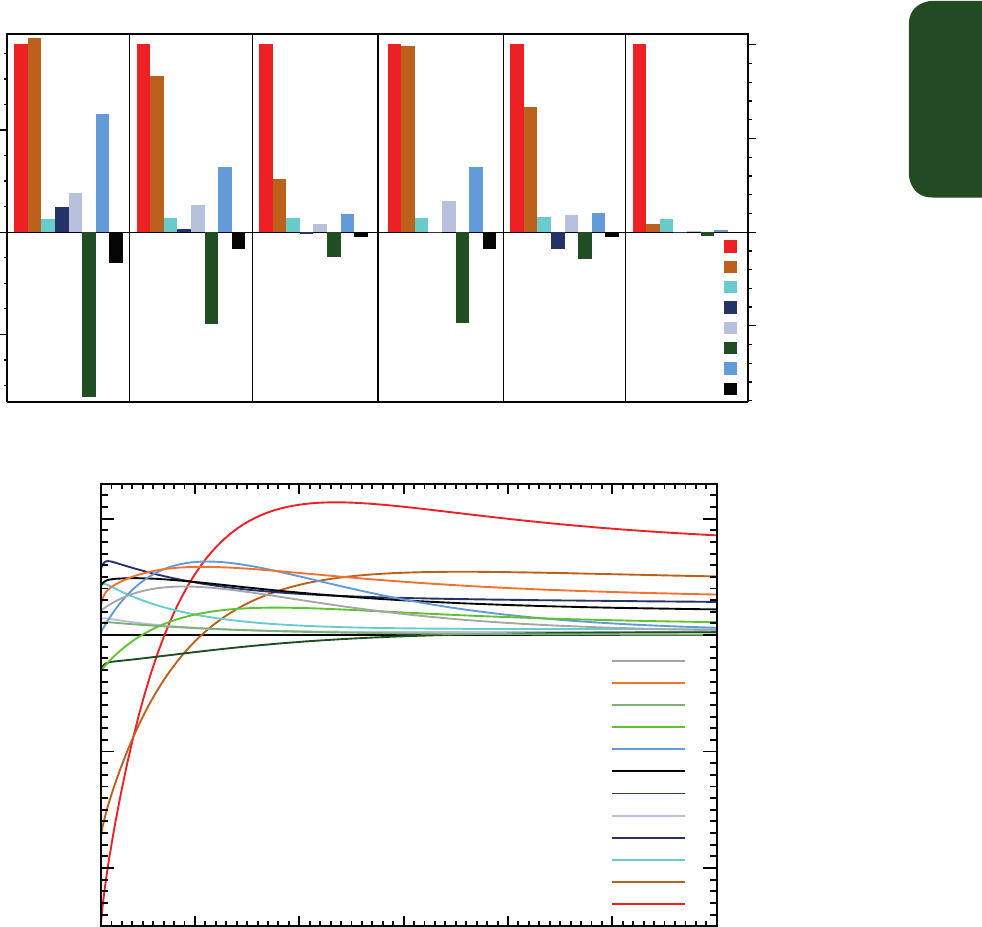
TS
Technical Summary
59
10 yrs 20 yrs 100 yrs
10 yrs
20 yrs 100 yrs
20
0
-20
5
10
0
-5
CO
2
equivalent emissions (Pg CO
2
-eq)
CO
2
equivalent emissions (PgC-eq)
GWP GTP
NO
X
CO
BC
OC
SO
2
CO
2
CH
4
N
2
O
Time Horizon (yr)
Temperature impact (10
-3
K)
10 20 30 40 50 60
-20
-10
0
10
Energy
Industry
Aviation
Road
Non-road
Shipping
Household fossil & biofuel
Animal husbandry
Agriculture
Agricultural waste burning
Biomass burning
Waste/landfill
Figure TS.8 | (Upper) Global anthropogenic present-day emissions weighted by the Global Warming Potential (GWP) and the Global Temperature change Potential (GTP) for the
chosen time horizons. Year 2008 (single-year pulse) emissions weighted by GWP, which is the global mean radiative forcing (RF) per unit mass emitted integrated over the indicated
number of years relative to the forcing from CO
2
emissions, and GTP which estimates the impact on global mean temperature based on the temporal evolution of both RF and cli-
mate response per unit mass emitted relative to the impact of CO
2
emissions. The units are ‘CO
2
equivalents’, which reflects equivalence only in the impact parameter of the chosen
metric (integrated RF over the chosen time horizon for GWP; temperature change at the chosen point in time for GTP), given as Pg(CO
2
)eq (left axis) and PgCeq (right axis). (Bottom)
The Absolute GTP (AGTP) as a function of time multiplied by the present-day emissions of all compounds from the indicated sectors is used to estimate global mean temperature
response (AGTP is the same as GTP, except is not normalized by the impact of CO
2
emissions). There is little change in the relative values for the sectors over the 60 to 100-year
time horizon. The effects of aerosol–cloud interactions and contrail-induced cirrus are not included in the upper panel. {Figures 8.32, 8.33}
shorter time horizons (up to about 20 years). Another useful perspec-
tive is to examine the effect of sustained current emissions. Because
emitted substances are removed according to their residence time,
short-lived species remain at nearly constant values while long-lived
gases accumulate in this analysis. In both cases, the sectors that have
the greatest long-term warming impacts (energy and industry) lead
to cooling in the near term (primarily due to SO
2
emissions), and thus
emissions from those sectors can lead to opposite global mean tem-
perature responses at short and long time scales. The relative impor-
tance of the other sectors depends on the time and perspective chosen.
As with RF or ERF, uncertainties in aerosol impacts are large, and in
particular attribution of aerosol–cloud interactions to individual com-
ponents is poorly constrained. {8.7; Chapter 8 Supplementary Material
Figures 8.SM.9, 8.SM.10}
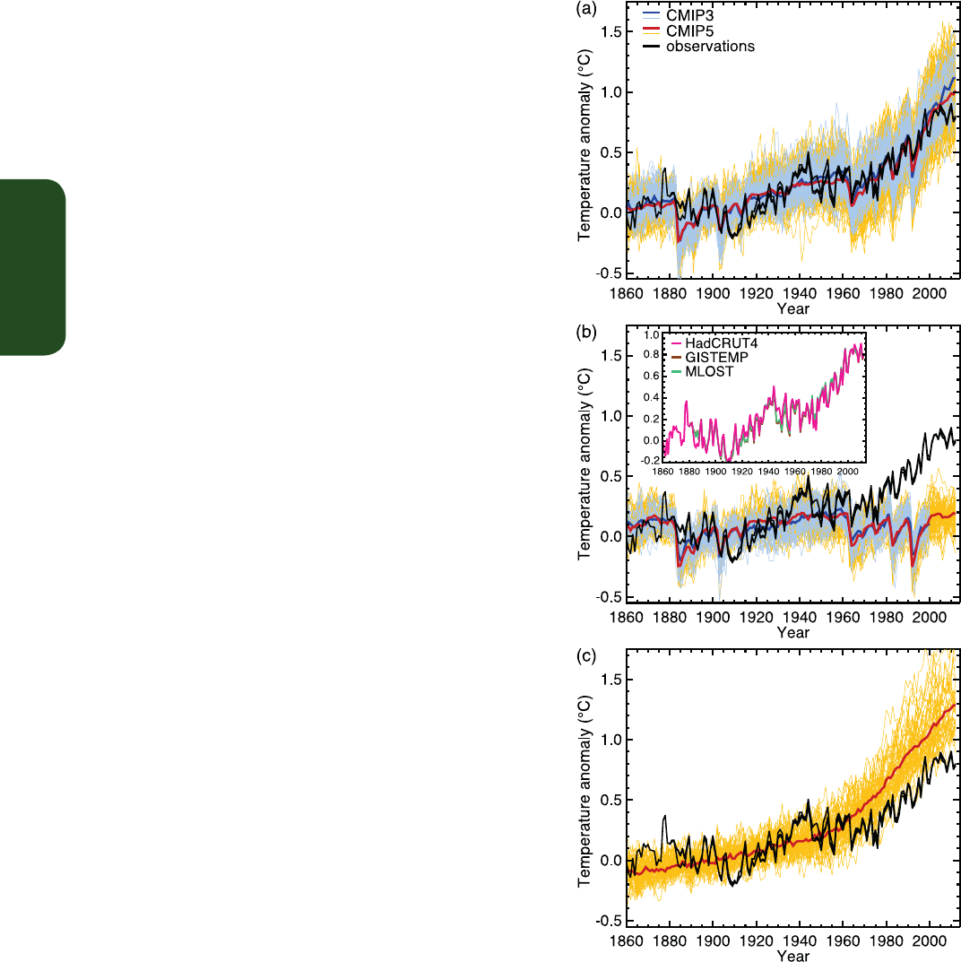
TS
Technical Summary
60
TS.4 Understanding the Climate System and
Its Recent Changes
TS.4.1 Introduction
Understanding of the climate system results from combining obser-
vations, theoretical studies of feedback processes and model simula-
tions. Compared to AR4, more detailed observations and improved
climate models (see Box TS.4) now enable the attribution of detected
changes to human influences in more climate system components.
The consistency of observed and modelled changes across the climate
system, including in regional temperatures, the water cycle, global
energy budget, cryosphere and oceans (including ocean acidification),
points to global climate change resulting primarily from anthropogenic
increases in WMGHG concentrations. {10}
TS.4.2 Surface Temperature
Several advances since the AR4 have allowed a more robust quantifica-
tion of human influence on surface temperature changes. Observational
uncertainty has been explored much more thoroughly than previously
and the assessment now considers observations from the first decade
of the 21st century and simulations from a new generation of climate
models whose ability to simulate historical climate has improved in
many respects relative to the previous generation of models consid-
ered in AR4. Observed GMST anomalies relative to 1880–1919 in recent
years lie well outside the range of GMST anomalies in CMIP5 simula-
tions with natural forcing only, but are consistent with the ensemble
of CMIP5 simulations including both anthropogenic and natural forc-
ing (Figure TS.9) even though some individual models overestimate
the warming trend, while others underestimate it. Simulations with
WMGHG changes only, and no aerosol changes, generally exhibit stron-
ger warming than has been observed (Figure TS.9). Observed temper-
ature trends over the period 1951–2010, which are characterized by
warming over most of the globe with the most intense warming over
the NH continents, are, at most observed locations, consistent with the
temperature trends in CMIP5 simulations including anthropogenic and
natural forcings and inconsistent with the temperature trends in CMIP5
simulations including natural forcings only. A number of studies have
investigated the effects of the Atlantic Multi-decadal Oscillation (AMO)
on GMST. Although some studies find a significant role for the AMO
in driving multi-decadal variability in GMST, the AMO exhibited little
trend over the period 1951–2010 on which the current assessments are
based, and the AMO is assessed with high confidence to have made
little contribution to the GMST trend between 1951 and 2010 (consider-
ably less than 0.1°C). {2.4, 9.8.1, 10.3; FAQ 9.1}
It is extremely likely that human activities caused more than half of the
observed increase in global average surface temperature from 1951 to
2010. This assessment is supported by robust evidence from multiple
studies using different methods. In particular, the temperature trend
attributable to all anthropogenic forcings combined can be more close-
ly constrained in multi-signal detection and attribution analyses. Uncer-
tainties in forcings and in climate models’ responses to those forcings,
together with difficulty in distinguishing the patterns of temperature
response due to WMGHGs and other anthropogenic forcings, prevent
as precise a quantification of the temperature changes attributable to
Figure TS.9 | Three observational estimates of global mean surface temperature (black
lines) from the Hadley Centre/Climatic Research Unit gridded surface temperature data
set 4 (HadCRUT4), Goddard Institute for Space Studies Surface Temperature Analysis
(GISTEMP), and Merged Land–Ocean Surface Temperature Analysis (MLOST), com-
pared to model simulations (CMIP3 models— thin blue lines and CMIP5 models—thin
yellow lines) with anthropogenic and natural forcings (a), natural forcings only (b) and
greenhouse gas forcing only (c). Thick red and blue lines are averages across all avail-
able CMIP5 and CMIP3 simulations respectively. All simulated and observed data were
masked using the HadCRUT4 coverage (as this data set has the most restricted spatial
coverage), and global average anomalies are shown with respect to 1880–1919, where
all data are first calculated as anomalies relative to 1961–1990 in each grid box. Inset
to (b) shows the three observational data sets distinguished by different colours. {Figure
10.1}

TS
Technical Summary
61
Box TS.3 | Climate Models and the Hiatus in Global Mean Surface Warming of the Past 15 Years
The observed GMST has shown a much smaller increasing linear trend over the past 15 years than over the past 30 to 60 years (Box
TS.3, Figure 1a, c). Depending on the observational data set, the GMST trend over 1998–2012 is estimated to be around one third to
one half of the trend over 1951–2012. For example, in HadCRUT4 the trend is 0.04°C per decade over 1998–2012, compared to 0.11°C
per decade over 1951–2012. The reduction in observed GMST trend is most marked in NH winter. Even with this ‘hiatus’ in GMST trend,
the decade of the 2000s has been the warmest in the instrumental record of GMST. Nevertheless, the occurrence of the hiatus in GMST
trend during the past 15 years raises the two related questions of what has caused it and whether climate models are able to reproduce
it. {2.4.3, 9.4.1; Box 9.2; Table 2.7}
Fifteen-year-long hiatus periods are common in both the observed and CMIP5 historical GMST time series. However, an analysis of the
full suite of CMIP5 historical simulations (augmented for the period 2006–2012 by RCP4.5 simulations) reveals that 111 out of 114
realizations show a GMST trend over 1998–2012 that is higher than the entire HadCRUT4 trend ensemble (Box TS.3, Figure 1a; CMIP5
ensemble mean trend is 0.21°C per decade). This difference between simulated and observed trends could be caused by some combina-
tion of (a) internal climate variability, (b) missing or incorrect RF, and (c) model response error. These potential sources of the difference,
which are not mutually exclusive, are assessed below, as is the cause of the observed GMST trend hiatus. {2.4.3, 9.3.2, 9.4.1; Box 9.2}
Internal Climate Variability
Hiatus periods of 10 to 15 years can arise as a manifestation of internal decadal climate variability, which sometimes enhances and
sometimes counteracts the long-term externally forced trend. Internal variability thus diminishes the relevance of trends over periods
as short as 10 to 15 years for long-term climate change. Furthermore, the timing of internal decadal climate variability is not expected
to be matched by the CMIP5 historical simulations, owing to the predictability horizon of at most 10 to 20 years (CMIP5 historical
simulations are typically started around nominally 1850 from a control run). However, climate models exhibit individual decades of
GMST trend hiatus even during a prolonged phase of energy uptake of the climate system, in which case the energy budget would be
balanced by increasing subsurface–ocean heat uptake. {2.4.3, 9.3.2, 11.2.2; Boxes 2.2, 9.2}
Owing to sampling limitations, it is uncertain whether an increase in the rate of subsurface–ocean heat uptake occurred during the past
15 years. However, it is very likely that the climate system, including the ocean below 700 m depth, has continued to accumulate energy
over the period 1998–2010. Consistent with this energy accumulation, GMSL has continued to rise during 1998–2012, at a rate only
slightly and insignificantly lower than during 1993–2012. The consistency between observed heat content and sea level changes yields
high confidence in the assessment of continued ocean energy accumulation, which is in turn consistent with the positive radiative
imbalance of the climate system. By contrast, there is limited evidence that the hiatus in GMST trend has been accompanied by a slower
rate of increase in ocean heat content over the depth range 0 to 700 m, when comparing the period 2003–2010 against 1971–2010.
There is low agreement on this slowdown, as three of five analyses show a slowdown in the rate of increase while the other two show
the increase continuing unabated. {3.2.3, 3.2.4, 3.7, 8.5.1, 13.3; Boxes 3.1, 13.1}
During the 15-year period beginning in 1998, the ensemble of HadCRUT4 GMST trends lies below almost all model-simulated trends
(Box TS.3, Figure 1a), whereas during the 15-year period ending in 1998, it lies above 93 out of 114 modelled trends (Box TS.3, Figure
1b; HadCRUT4 ensemble mean trend 0.26°C per decade, CMIP5 ensemble mean trend 0.16°C per decade). Over the 62-year period
1951–2012, observed and CMIP5 ensemble mean trend agree to within 0.02°C per decade (Box TS.3, Figure 1c; CMIP5 ensemble mean
trend 0.13°C per decade). There is hence very high confidence that the CMIP5 models show long-term GMST trends consistent with
observations, despite the disagreement over the most recent 15-year period. Due to internal climate variability, in any given 15-year
period the observed GMST trend sometimes lies near one end of a model ensemble, an effect that is pronounced in Box TS.3, Figure 1a,
b as GMST was influenced by a very strong El Niño event in 1998. {Box 9.2}
Unlike the CMIP5 historical simulations referred to above, some CMIP5 predictions were initialized from the observed climate state
during the late 1990s and the early 21st century. There is medium evidence that these initialized predictions show a GMST lower by about
0.05°C to 0.1°C compared to the historical (uninitialized) simulations and maintain this lower GMST during the first few years of the sim-
ulation. In some initialized models this lower GMST occurs in part because they correctly simulate a shift, around 2000, from a positive to
a negative phase of the Inter-decadal Pacific Oscillation (IPO). However, the improvement of this phasing of the IPO through initialization
is not universal across the CMIP5 predictions. Moreover, although part of the GMST reduction through initialization indeed results from
initializing at the correct phase of internal variability, another part may result from correcting a model bias that was caused by incorrect
past forcing or incorrect model response to past forcing, especially in the ocean. The relative magnitudes of these effects are at present
unknown; moreover, the quality of a forecasting system cannot be evaluated from a single prediction (here, a 10-year prediction within
(continued on next page)

TS
Technical Summary
62
Box TS.3 (continued)
the period 1998–2012). Overall, there is medium confidence that initialization leads to simulations of GMST during 1998–2012 that are
more consistent with the observed trend hiatus than are the uninitialized CMIP5 historical simulations, and that the hiatus is in part a
consequence of internal variability that is predictable on the multi-year time scale. {11.1, 11.2.3; Boxes 2.5, 9.2, 11.1, 11.2}
Radiative Forcing
On decadal to interdecadal time scales and under continually increasing ERF, the forced component of the GMST trend responds to the
ERF trend relatively rapidly and almost linearly (medium confidence). The expected forced-response GMST trend is related to the ERF
trend by a factor that has been estimated for the 1% per year CO
2
increases in the CMIP5 ensemble as 2.0 [1.3 to 2.7] W m
–2
ºC
–1
(90%
uncertainty range). Hence, an ERF trend can be approximately converted to a forced-response GMST trend, permitting an assessment
of how much of the change in the GMST trends shown in Box TS.3, Figure 1 is due to a change in ERF trend. {Box 9.2}
The AR5 best-estimate ERF trend over 1998–2011 is 0.22 [0.10 to 0.34] W m
–2
per decade (90% uncertainty range), which is substan-
tially lower than the trend over 1984–1998 (0.32 [0.22 to 0.42] W m
–2
per decade; note that there was a strong volcanic eruption in
1982) and the trend over 1951–2011 (0.31 [0.19 to 0.40] W m
–2
per decade; Box TS.3, Figure 1d–f; the end year 2011 is chosen because
data availability is more limited than for GMST). The resulting forced-response GMST trend would approximately be 0.12 [0.05 to 0.29]
ºC per decade, 0.19 [0.09 to 0.39] ºC per decade, and 0.18 [0.08 to 0.37] ºC per decade for the periods 1998–2011, 1984–1998, and
1951–2011, respectively (the uncertainty ranges assume that the range of the conversion factor to GMST trend and the range of ERF
trend itself are independent). The AR5 best-estimate ERF forcing trend difference between 1998–2011 and 1951–2011 thus might
explain about one-half (0.05 ºC per decade) of the observed GMST trend difference between these periods (0.06 to 0.08 ºC per decade,
depending on observational data set). {8.5.2}
The reduction in AR5 best-estimate ERF trend over 1998–2011 compared to both 1984–1998 and 1951–2011 is mostly due to decreas-
ing trends in the natural forcings, –0.16 [–0.27 to –0.06] W m
–2
per decade over 1998–2011 compared to 0.01 [–0.00 to +0.01] W m
–2
per decade over 1951–2011. Solar forcing went from a relative maximum in 2000 to a relative minimum in 2009, with a peak-to-peak
difference of around 0.15 W m
–2
and a linear trend over 1998–2011 of around –0.10 W m
–2
per decade. Furthermore, a series of small
volcanic eruptions has increased the observed stratospheric aerosol loading after 2000, leading to an additional negative ERF linear-
trend contribution of around –0.06 W m
–2
per decade over 1998–2011 (Box TS.3, Figure 1d, f). By contrast, satellite-derived estimates
of tropospheric aerosol optical depth suggests little overall trend in global mean aerosol optical depth over the last 10 years, implying
little change in ERF due to aerosol–radiative interaction (low confidence because of low confidence in aerosol optical depth trend
itself). Moreover, because there is only low confidence in estimates of ERF due to aerosol–cloud interaction, there is likewise low con-
fidence in its trend over the last 15 years. {2.2.3, 8.4.2, 8.5.1, 8.5.2, 10.3.1; Box 10.2; Table 8.5}
For the periods 1984–1998 and 1951–2011, the CMIP5 ensemble mean ERF trend deviates from the AR5 best-estimate ERF trend by
only 0.01 W m
–2
per decade (Box TS.3, Figure 1e, f). After 1998, however, some contributions to a decreasing ERF trend are missing in
the CMIP5 models, such as the increasing stratospheric aerosol loading after 2000 and the unusually low solar minimum in 2009. None-
theless, over 1998–2011 the CMIP5 ensemble mean ERF trend is lower than the AR5 best-estimate ERF trend by 0.03 W m
–2
per decade
(Box TS.3, Figure 1d). Furthermore, global mean aerosol optical depth in the CMIP5 models shows little trend over 1998–2012, similar
to the observations. Although the forcing uncertainties are substantial, there are no apparent incorrect or missing global mean forcings
in the CMIP5 models over the last 15 years that could explain the model–observations difference during the warming hiatus. {9.4.6}
Model Response Error
The discrepancy between simulated and observed GMST trends during 1998–2012 could be explained in part by a tendency for some
CMIP5 models to simulate stronger warming in response to increases in greenhouse-gas concentration than is consistent with obser-
vations. Averaged over the ensembles of models assessed in Section 10.3.1, the best-estimate GHG and other anthropogenic scaling
factors are less than one (though not significantly so, Figure 10.4), indicating that the model-mean GHG and other anthropogenic respons-
es should be scaled down to best match observations. This finding provides evidence that some CMIP5 models show a larger response to
GHGs and other anthropogenic factors (dominated by the effects of aerosols) than the real world (medium confidence). As a consequence,
it is argued in Chapter 11 that near-term model projections of GMST increase should be scaled down by about 10%. This downward scal-
ing is, however, not sufficient to explain the model mean overestimate of GMST trend over the hiatus period. {10.3.1, 11.3.6}
Another possible source of model error is the poor representation of water vapour in the upper atmosphere. It has been suggested that
a reduction in stratospheric water vapour after 2000 caused a reduction in downward longwave radiation and hence a surface-cooling
contribution, possibly missed by the models. However, this effect is assessed here to be small, because there was a recovery in strato-
spheric water vapour after 2005. {2.2.2, 9.4.1; Box 9.2} (continued on next page)
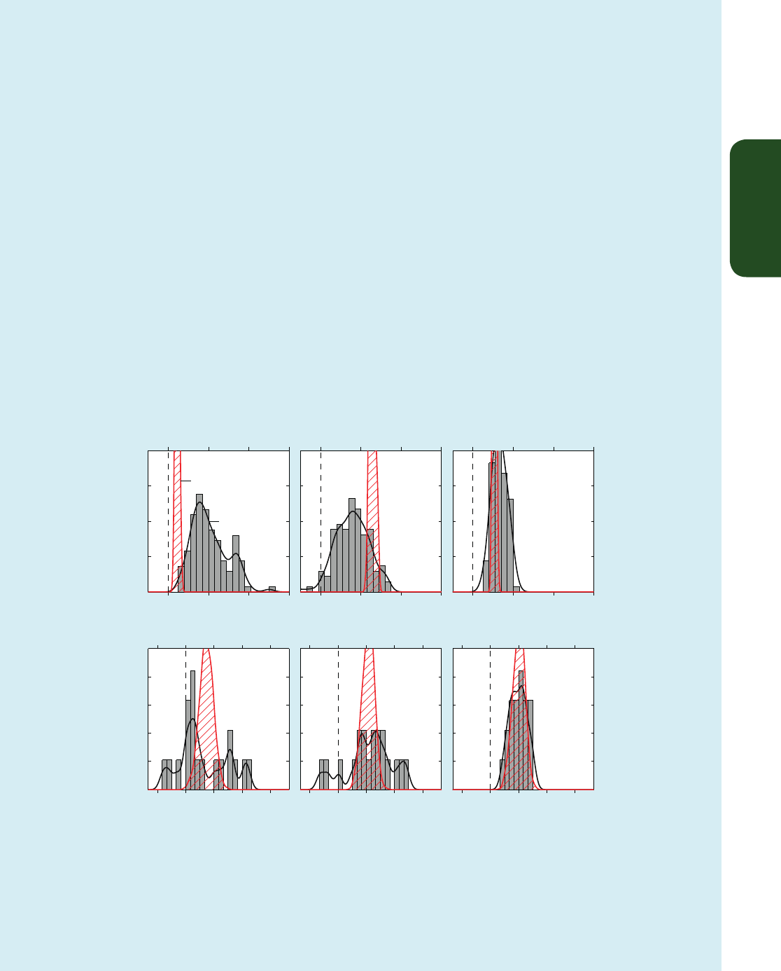
TS
Technical Summary
63
Box TS.3 (continued)
In summary, the observed recent warming hiatus, defined as the reduction in GMST trend during 1998–2012 as compared to the trend
during 1951–2012, is attributable in roughly equal measure to a cooling contribution from internal variability and a reduced trend in
external forcing (expert judgement, medium confidence). The forcing trend reduction is due primarily to a negative forcing trend from
both volcanic eruptions and the downward phase of the solar cycle. However, there is low confidence in quantifying the role of forcing
trend in causing the hiatus, because of uncertainty in the magnitude of the volcanic forcing trend and low confidence in the aerosol
forcing trend. {Box 9.2}
Almost all CMIP5 historical simulations do not reproduce the observed recent warming hiatus. There is medium confidence that the GMST
trend difference between models and observations during 1998–2012 is to a substantial degree caused by internal variability, with pos-
sible contributions from forcing error and some CMIP5 models overestimating the response to increasing GHG forcing. The CMIP5 model
trend in ERF shows no apparent bias against the AR5 best estimate over 1998–2012. However, confidence in this assessment of CMIP5
ERF trend is low, primarily because of the uncertainties in model aerosol forcing and processes, which through spatial heterogeneity
might well cause an undetected global mean ERF trend error even in the absence of a trend in the global mean aerosol loading. {Box 9.2}
The causes of both the observed GMST trend hiatus and of the model–observation GMST trend difference during 1998–2012 imply
that, barring a major volcanic eruption, most 15-year GMST trends in the near-term future will be larger than during 1998–2012 (high
confidence; see Section 11.3.6 for a full assessment of near-term projections of GMST). The reasons for this implication are fourfold:
first, anthropogenic GHG concentrations are expected to rise further in all RCP scenarios; second, anthropogenic aerosol concentration
is expected to decline in all RCP scenarios, and so is the resulting cooling effect; third, the trend in solar forcing is expected to be larger
over most near-term 15-year periods than over 1998–2012 (medium confidence), because 1998–2012 contained the full downward
phase of the solar cycle; and fourth, it is more likely than not that internal climate variability in the near term will enhance and not
counteract the surface warming expected to arise from the increasing anthropogenic forcing. {Box 9.2}
Box TS.3, Figure 1 | (Top) Observed and simulated GMST trends in °C per decade, over the periods 1998–2012 (a), 1984–1998 (b), and 1951–2012 (c). For the
observations, 100 realizations of the Hadley Centre/Climatic Research Unit gridded surface temperature data set 4 (HadCRUT4) ensemble are shown (red, hatched). The
uncertainty displayed by the ensemble width is that of the statistical construction of the global average only, in contrast to the trend uncertainties quoted in Section
2.4.3, which include an estimate of internal climate variability. Here, by contrast, internal variability is characterized through the width of the model ensemble. For the
models, all 114 available CMIP5 historical realizations are shown, extended after 2005 with the RCP4.5 scenario and through 2012 (grey, shaded). (Bottom) Trends
in effective radiative forcing (ERF, in W m
–2
per decade) over the periods 1998–2011 (d), 1984–1998 (e), and 1951–2011 (f). The figure shows AR5 best-estimate ERF
trends (red, hatched) and CMIP5 ERF (grey, shaded). Black lines are smoothed versions of the histograms. Each histogram is normalized so that its area sums up to one.
{2.4.3, 8.5.2; Box 9.2; Figure 8.18; Box 9.2, Figure 1}
1998-2012
0.0 0.2 0.4 0.6
(°C per decade) (°C per decade)(°C per decade)
0
2
4
6
8
Normalized density
CMIP5
HadCRUT4
(a)
1984-1998
0.0 0.2 0.4 0.6
(b)
1951-2012
0.0 0.2 0.4 0.6
(c)
1998-2011
-0.3 0.0 0.3 0.6 0.9
(W m
-2
per decade) (W m
-2
per decade) (W m
-2
per decade)
0
1
2
3
4
5
Normalized density
(d)
1984-1998
-0.3 0.0 0.3 0.6 0.9
(e)
1951-2011
-0.3 0.0 0.3 0.6 0.9
(f)
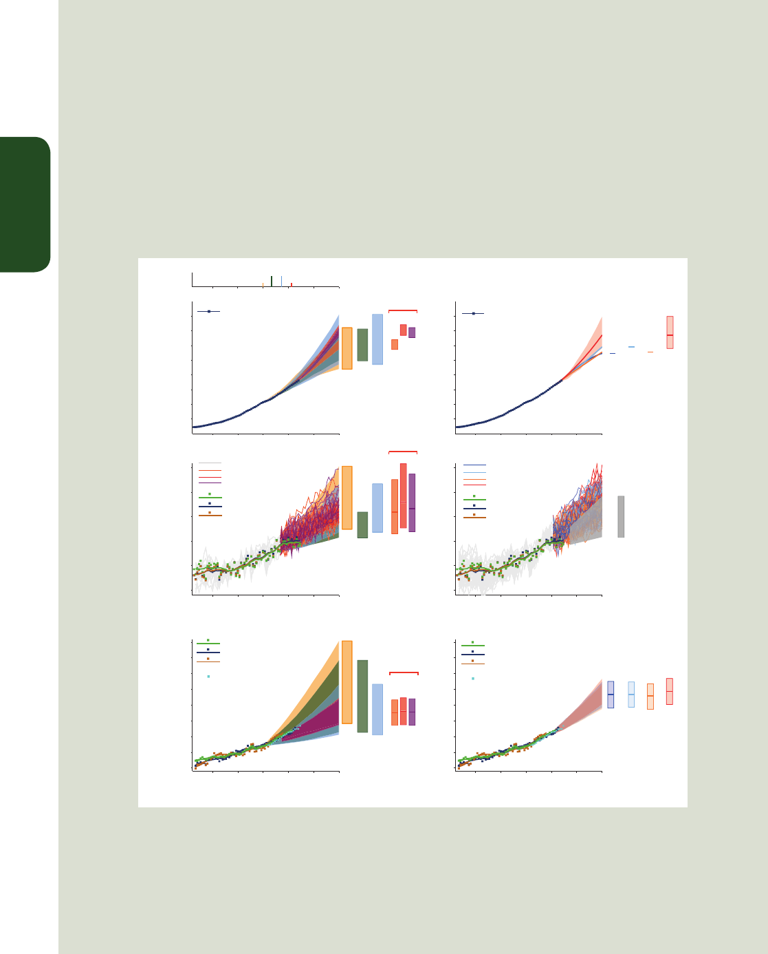
TS
Technical Summary
64
Thematic Focus Elements
TFE.3 | Comparing Projections from Previous IPCC Assessments with Observations
Verification of projections is arguably the most convincing way of establishing the credibility of climate change
science. Results of projected changes in carbon dioxide (CO
2
), global mean surface temperature (GMST) and global
mean sea level (GMSL) from previous IPCC assessment reports are quantitatively compared with the best available
observational estimates. The comparison between the four previous reports highlights the evolution in our under-
standing of how the climate system responds to changes in both natural and anthropogenic forcing and provides
an assessment of how the projections compare with observational estimates. TFE.3, Figure 1, for example, shows the
projected and observed estimates of: (1) CO
2
changes (top row), (2) GMST anomaly relative to 1961–1990 (middle
row) and (3) GMSL relative to 1961–1990 (bottom row). Results from previous assessment reports are in the left-
hand column, and for completeness results from current assessment are given in the right-hand column. {2.4, 3.7,
6.3, 11.3, 13.3} (continued on next page)
TFE.3, Figure 1 | (Top left) Observed globally and annually averaged CO
2
concentrations in parts per million (ppm) since 1950 compared with projections from the
previous IPCC assessments. Observed global annual CO
2
concentrations are shown in dark blue. The shading shows the largest model projected range of global annual
CO
2
concentrations from 1950 to 2035 from FAR (First Assessment Report; Figure A.3 in the Summary for Policymakers (SPM) of IPCC 1990), SAR (Second Assessment
Report; Figure 5b in the TS of IPCC 1996), TAR (Third Assessment Report; Appendix II of IPCC 2001), and for the IPCC Special Report on Emission Scenarios (SRES) A2,
A1B and B1 scenarios presented in the AR4 (Fourth Assessment Report; Figure 10.26). The publication years of the assessment reports are shown. (Top right) Same
observed globally averaged CO
2
concentrations and the projections from this report. Only RCP8.5 has a range of values because the emission-driven senarios were
carried out only for this RCP. For the other RCPs the best estimate is given. (Middle left) Estimated changes in the observed globally and annually averaged surface
temperature anomaly relative to 1961–1990 (in °C) since 1950 compared with the range of projections from the previous IPCC assessments. Values are harmonized
TARSAR
FAR
AR4
1960 1975 1990 2005 2020 2035
325
350
375
400
425
450
475
500
CO
2
concentration
(ppm)
1960 1975 1990 2005 2020 2035
325
350
375
400
425
450
475
500
1960 1975 1990 2005 2020 2035
−0.5
0
0.5
1
1.5
2
Temperature anomaly (°C)
w.r.t. 1961−1990
1960 1975 1990 2005 2020 2035
−0.5
0
0.5
1
1.5
2
1960 1975 1990 2005 2020 2035
−5
0
5
10
15
20
25
30
35
Global mean
sea level rise (cm)
1960 1975 1990 2005 2020 2035
−5
0
5
10
15
20
25
30
35
FAR
SAR
TAR
A1B
A2
B1
FAR
SAR
TAR
A1B
A2
B1
AR4
AR4
Post-AR4
FAR
SAR
TAR
A1B
A2
B1
Observations
AR4 CMIP3
}
Observations
}
Estimates derived from
sea-surface altimetry
Estimates derived
from tide-gauge data
}
RCP
8.5
RCP
6.0
RCP
4.5
RCP
2.6
Observations
AR5 CMIP5
}
Observations
}
Estimates derived from
sea-surface altimetry
Estimates derived
from tide-gauge data
}
RCP
6.0
RCP
4.5
RCP
2.6
RCP
8.5
Indicative
likely
range
Year Year

TS
Technical Summary
65
Carbon Dioxide Changes
From 1950 to 2011 the observed concentrations of atmospheric CO
2
have steadily increased. Considering the period
1990–2011, the observed CO
2
concentration changes lie within the envelope of the scenarios used in the four
assessment reports. As the most recent assessment prior to the current, the IPCC Fourth Assessment Report (AR4)
(TFE.3.Figure 1; top left) has the narrowest scenario range and the observed concentration follows this range. The
results from the IPCC Fifth Assessment Report (AR5) (TFE.3, Figure 1; top right) are consistent with AR4, and during
2002–2011, atmospheric CO
2
concentrations increased at a rate of 1.9 to 2.1 ppm yr
–1
. {2.2.1, 6.3; Table 6.1}
Global Mean Temperature Anomaly
Relative to the 1961–1990 mean, the GMST anomaly has been positive and larger than 0.25°C since 2001. Observa-
tions are generally well within the range of the extent of the earlier IPCC projections (TFE.3, Figure1, middle left)
This is also true for the Coupled Model Intercomparison Project Phase 5 (CMIP5) results (TFE.3, Figure 1; middle
right) in the sense that the observed record lies within the range of the model projections, but on the lower end of
the plume. Mt Pinatubo erupted in 1991 (see FAQ 11.2 for discussion of how volcanoes impact the climate system),
leading to a brief period of relative global mean cooling during the early 1990s. The IPCC First, Second and Third
Assessment Reports (FAR, SAR and TAR) did not include the effects of volcanic eruptions and thus failed to include
the cooling associated with the Pinatubo eruption. AR4 and AR5, however, did include the effects from volcanoes
and did simulate successfully the associated cooling. During 1995–2000 the global mean temperature anomaly was
quite variable—a significant fraction of this variability was due to the large El Niño in 1997–1998 and the strong
back-to-back La Niñas in 1999–2001. The projections associated with these assessment reports do not attempt to
capture the actual evolution of these El Niño and La Niña events, but include them as a source of uncertainty due
to natural variability as encompassed by, for example, the range given by the individual CMIP3 and CMIP5 simula-
tions and projection (TFE.3, Figure 1). The grey wedge in TFE.3, Figure 1 (middle right) corresponds to the indicative
likely range for annual temperatures, which is determined from the Representative Concentration Pathways (RCPs)
assessed value for the 20-year mean 2016–2035 (see discussion of Figure TS.14 and Section 11.3.6 for details). From
1998 to 2012 the observational estimates have largely been on the low end of the range given by the scenarios
alone in previous assessment reports and CMIP3 and CMIP5 projections. {2.4; Box 9.2}
Global Mean Sea Level
Based on both tide gauge and satellite altimetry data, relative to 1961–1990, the GMSL has continued to rise. While
the increase is fairly steady, both observational records show short periods of either no change or a slight decrease.
The observed estimates lie within the envelope of all the projections except perhaps in the very early 1990s. The
sea level rise uncertainty due to scenario-related uncertainty is smallest for the most recent assessments (AR4 and
AR5) and observed estimates lie well within this scenario-related uncertainty. It is virtually certain that over the 20th
century sea level rose. The mean rate of sea level increase was 1.7 mm yr
–1
with a very likely range between 1.5 to
1.9 between 1901 and 2010 and this rate increased to 3.2 with a likely range of 2.8 to 3.6 mm yr
–1
between 1993
and 2010 (see TFE.2). {3.7.2, 3.7.4}
TFE.3 (continued)
to start from the same value at 1990. Observed global annual temperature anomaly, relative to 1961–1990, from three data sets is shown as squares and smoothed
time series as solid lines from the Hadley Centre/Climatic Research Unit gridded surface temperature data set 4 (HadCRUT4; bright green), Merged Land–Ocean Surface
Temperature Analysis (MLOST; warm mustard) and Goddard Institute for Space Studies Surface Temperature Analysis (GISTEMP; dark blue) data sets. The coloured
shading shows the projected range of global annual mean near surface temperature change from 1990 to 2035 for models used in FAR (Figure 6.11), SAR (Figure 19 in
the TS of IPCC 1996), TAR (full range of TAR, Figure 9.13(b)). TAR results are based on the simple climate model analyses presented in this assessment and not on the
individual full three-dimensional climate model simulations. For the AR4 results are presented as single model runs of the CMIP3 ensemble for the historical period from
1950 to 2000 (light grey lines) and for three SRES scenarios (A2, A1B and B1) from 2001 to 2035. For the three SRES scenarios the bars show the CMIP3 ensemble
mean and the likely range given by –40 % to +60% of the mean as assessed in Chapter 10 of AR4. (Middle right) Projections of annual mean global mean surface air
temperature (GMST) for 1950–2035 (anomalies relative to 1961–1990) under different RCPs from CMIP5 models (light grey and coloured lines, one ensemble member
per model), and observational estimates the same as the middle left panel. The grey shaded region shows the indicative likely range for annual mean GMST during
the period 2016–2035 for all RCPs (see Figure TS.14 for more details). The grey bar shows this same indicative likely range for the year 2035. (Bottom left) Estimated
changes in the observed global annual mean sea level (GMSL) since 1950. Different estimates of changes in global annual sea level anomalies from tide gauge data
(dark blue, warm mustard, dark green) and based on annual averages of altimeter data (light blue ) starting in 1993 (the values have been aligned to fit the 1993 value
of the tide gauge data). Squares indicate annual mean values, solid lines smoothed values. The shading shows the largest model projected range of global annual sea
level rise from 1950 to 2035 for FAR (Figures 9.6 and 9.7), SAR (Figure 21 in TS of IPCC, 1996), TAR (Appendix II of IPCC, 2001) and based on the CMIP3 model results
available at the time of AR4 using the SRES A1B scenario. Note that in the AR4 no full range was given for the sea level projections for this period. Therefore, the figure
shows results that have been published subsequent to the AR4. The bars at the right hand side of each graph show the full range given for 2035 for each assessment
report. (Bottom right) Same observational estimate as bottom left. The bars are the likely ranges (medium confidence) for global mean sea level rise at 2035 with respect
to 1961–1990 following the four RCPs. Appendix 1.A provides details on the data and calculations used to create these figures. See Chapters 1, 11 and 13 for more
details. {Figures 1.4, 1.5, 1.10, 11.9, 11.19, 11.25, 13.11}
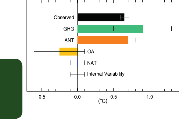
TS
Technical Summary
66
WMGHGs and other anthropogenic forcings individually. Consistent
with AR4, it is assessed that more than half of the observed increase
in global average surface temperature from 1951 to 2010 is very likely
due to the observed anthropogenic increase in WMGHG concentra-
tions. WMGHGs contributed a global mean surface warming likely
to be between 0.5°C and 1.3°C over the period between 1951 and
2010, with the contributions from other anthropogenic forcings likely
to be between –0.6°C and 0.1°C and from natural forcings likely to be
between –0.1°C and 0.1°C. Together these assessed contributions are
consistent with the observed warming of approximately 0.6°C over
this period (Figure TS.10). {10.3}
Solar forcing is the only known natural forcing acting to warm the
climate over the 1951–2010 period but it has increased much less
than WMGHG forcing, and the observed pattern of long-term tropo-
spheric warming and stratospheric cooling is not consistent with the
expected response to solar irradiance variations. Considering this
evidence together with the assessed contribution of natural forcings
to observed trends over this period, it is assessed that the contribu-
tion from solar forcing to the observed global warming since 1951
is extremely unlikely to be larger than that from WMGHGs. Because
solar forcing has very likely decreased over a period with direct satel-
lite measurements of solar output from 1986 to 2008, there is high
confidence that changes in total solar irradiance have not contributed
to global warming during that period. However, there is medium con-
fidence that the 11-year cycle of solar variability influences decadal
climate fluctuations in some regions through amplifying mechanisms.
{8.4, 10.3; Box 10.2}
Observed warming over the past 60 years is far outside the range of
internal climate variability estimated from pre-instrumental data, and it
is also far outside the range of internal variability simulated in climate
models. Model-based simulations of internal variability are assessed to
be adequate to make this assessment. Further, the spatial pattern of
observed warming differs from those associated with internal variabil-
ity. Based on this evidence, the contribution of internal variability to
the 1951–2010 GMST trend was assessed to be likely between –0.1°C
and 0.1°C, and it is virtually certain that warming since 1951 cannot be
explained by internal variability alone. {9.5, 10.3, 10.7}
The instrumental record shows a pronounced warming during the first
half of the 20th century. Consistent with AR4, it is assessed that the
early 20th century warming is very unlikely to be due to internal vari-
ability alone. It remains difficult to quantify the contributions to this
early century warming from internal variability, natural forcing and
anthropogenic forcing, due to forcing and response uncertainties and
incomplete observational coverage. {10.3}
TS.4.3 Atmospheric Temperature
A number of studies since the AR4 have investigated the consistency of
simulated and observed trends in free tropospheric temperatures (see
section TS.2). Most, though not all, CMIP3 and CMIP5 models overes-
timate the observed warming trend in the tropical troposphere during
the satellite period 1979–2012. Roughly one half to two thirds of this
difference from the observed trend is due to an overestimate of the
SST trend, which is propagated upward because models attempt to
maintain static stability. There is low confidence in these assessments,
however, owing to the low confidence in observed tropical tropospher-
ic trend rates and vertical structure. Outside the tropics, and over the
period of the radiosonde record beginning in 1961, the discrepancy
between simulated and observed trends is smaller. {2.4.4, 9.4, 10.3}
Analysis of both radiosonde and satellite data sets, combined with
CMIP5 and CMIP3 simulations, continues to find that observed tro-
pospheric warming is inconsistent with internal variability and simu-
lations of the response to natural forcings alone. Over the period
1961–2010 CMIP5 models simulate tropospheric warming driven
by WMGHG changes, with only a small offsetting cooling due to the
combined effects of changes in reflecting and absorbing aerosols and
tropospheric ozone. Taking this evidence together with the results of
multi-signal detection and attribution analyses, it is likely that anthro-
pogenic forcings, dominated by WMGHGs, have contributed to the
warming of the troposphere since 1961. Uncertainties in radiosonde
and satellite records makes assessment of causes of observed trends in
the upper troposphere less confident than an assessment of the overall
atmospheric temperature changes. {2.4.4, 9.4, 10.3}
CMIP5 simulations including WMGHGs, ozone and natural forcing
changes broadly reproduce the observed evolution of lower strato-
spheric temperature, with some tendency to underestimate the
observed cooling trend over the satellite era (see Section TS.2). New
studies of stratospheric temperature, considering the responses to nat-
ural forcings, WMGHGs and ozone-depleting substances, demonstrate
that it is very likely that anthropogenic forcings, dominated by the
depletion of the ozone layer due to ozone depleting substances have
contributed to the cooling of the lower stratosphere since 1979. CMIP5
models simulate only a very weak cooling of the lower stratosphere in
response to historical WMGHG changes, and the influence of WMGHGs
on lower stratospheric temperature has not been formally detected.
Considering both regions together, it is very likely that anthropogenic
Figure TS.10 | Assessed likely ranges (whiskers) and their midpoints (bars) for warming
trends over the 1951–2010 period due to well-mixed greenhouse gases (GHG), anthro-
pogenic forcings (ANT) anthropogenic forcings other than well-mixed greenhouse gases
(OA), natural forcings (NAT) and internal variability. The trend in the Hadley Centre/
Climatic Research Unit gridded surface temperature data set 4 (HadCRUT4) observa-
tions is shown in black with its 5 to 95% uncertainty range due only to observational
uncertainty in this record. {Figure 10.5}

TS
Technical Summary
67
Thematic Focus Elements
TFE.4 | The Changing Energy Budget of the Global Climate System
The global energy budget is a fundamental aspect of the Earth’s climate system and depends on many phenomena
within it. The ocean has stored about 93% of the increase in energy in the climate system over recent decades,
resulting in ocean thermal expansion and hence sea level rise. The rate of storage of energy in the Earth system
must be equal to the net downward radiative flux at the top of the atmosphere, which is the difference between
effective radiative forcing (ERF) due to changes imposed on the system and the radiative response of the system.
There are also significant transfers of energy between components of the climate system and from one location to
another. The focus here is on the Earth’s global energy budget since 1970, when better global observational data
coverage is available. {3.7, 9.4, 13.4; Box 3.1}
The ERF of the climate system has been positive as a result of increases in well-mixed (long-lived) greenhouse gas
(GHG) concentrations, changes in short-lived GHGs (tropospheric and stratospheric ozone and stratospheric water
vapour), and an increase in solar irradiance (TFE.4, Figure 1a). This has been partly compensated by a negative
contribution to the ERF of the climate system as a result of changes in tropospheric aerosol, which predominantly
reflect sunlight and furthermore enhance the brightness of clouds, although black carbon produces positive forc-
ing. Explosive volcanic eruptions (such as El Chichón in Mexico in 1982 and Mt Pinatubo in the Philippines in 1991)
(continued on next page)
TFE.4, Figure 1 | The Earth’s energy budget from 1970 through 2011. (a) The cumulative energy inflow into the Earth system from changes in well-mixed and short-
lived greenhouse gases, solar forcing, tropospheric aerosol forcing, volcanic forcing and changes in surface albedo due to land use change (all relative to 1860–1879)
are shown by the coloured lines; these contributions are added to give the total energy inflow (black; contributions from black carbon on snow and contrails as well
as contrail-induced cirrus are included but not shown separately). (b) The cumulative total energy inflow from (a, black) is balanced by the sum of the energy uptake
of the Earth system (blue; energy absorbed in warming the ocean, the atmosphere and the land, as well as in the melting of ice) and an increase in outgoing radiation
inferred from changes in the global mean surface temperature. The sum of these two terms is given for a climate feedback parameter α of 2.47, 1.23 and 0.82 W m
–2
°C
–1
, corresponding to an equilibrium climate sensitivity of 1.5°C, 3.0°C and 4.5°C, respectively; 1.5°C to 4.5°C is assessed to be the likely range of equilibrium climate
sensitivity. The energy budget would be closed for a particular value of α if the corresponding line coincided with the total energy inflow. For clarity, all uncertainties
(shading) shown are likely ranges. {Box 12.2; Box 13.1, Figure 1}
Year Year

TS
Technical Summary
68
forcing, particularly WMGHGs and stratospheric ozone depletion, has
led to a detectable observed pattern of tropospheric warming and
lower stratospheric cooling since 1961. {2.4, 9.4, 10.3}
TS.4.4 Oceans
The observed upper-ocean warming during the late 20th and early 21st
centuries and its causes have been assessed more completely since
AR4 using updated observations and more simulations (see Section
TS.2.2). The long term trends and variability in the observations are
most consistent with simulations of the response to both anthropo-
genic forcing and volcanic forcing. The anthropogenic fingerprint in
observed upper-ocean warming, consisting of global mean and basin-
scale pattern changes, has also been detected. This result is robust to
a number of observational, model and methodological or structural
uncertainties. It is very likely that anthropogenic forcings have made
can inject sulphur dioxide into the stratosphere, giving rise to stratospheric aerosol, which persists for several years.
Stratospheric aerosol reflects some of the incoming solar radiation and thus gives a negative forcing. Changes in
surface albedo from land use change have also led to a greater reflection of shortwave radiation back to space and
hence a negative forcing. Since 1970, the net ERF of the climate system has increased, and the integrated impact of
these forcings is an energy inflow over this period (TFE.4, Figure 1a). {2.3, 8.5; Box 13.1}
As the climate system warms, energy is lost to space through increased outgoing radiation. This radiative response
by the system is due predominantly to increased thermal radiation, but it is modified by climate feedbacks such as
changes in water vapour, clouds and surface albedo, which affect both outgoing longwave and reflected shortwave
radiation. The top of the atmosphere fluxes have been measured by the Earth Radiation Budget Experiment (ERBE)
satellites from 1985 to 1999 and the Cloud and the Earth’s Radiant Energy System (CERES) satellites from March
2000 to the present. The top of the atmosphere radiative flux measurements are highly precise, allowing identifi-
cation of changes in the Earth’s net energy budget from year to year within the ERBE and CERES missions, but the
absolute calibration of the instruments is not sufficiently accurate to allow determination of the absolute top of
the atmosphere energy flux or to provide continuity across missions. TFE.4, Figure 1b relates the cumulative total
energy change of the Earth system to the change in energy storage and the cumulative outgoing radiation. Calcu-
lation of the latter is based on the observed global mean surface temperature multiplied by the climate feedback
parameter α, which in turn is related to the equilibrium climate sensitivity. The mid-range value for α, 1.23 W m
–2
°C
–1
, corresponds to an ERF for a doubled carbon dioxide (CO
2
) concentration of 3.7 [2.96 to 4.44] W m
–2
combined
with an equilibrium climate sensitivity of 3.0°C. The climate feedback parameter α is likely to be in the range from
0.82 to 2.47 W m
–2
°C
–1
(corresponding to the likely range in equilibrium climate sensitivity of 1.5°C to 4.5°C). {9.7.1;
Box 12.2}
If ERF were fixed, the climate system would eventually warm sufficiently that the radiative response would balance
the ERF, and there would be no further change in energy storage in the climate system. However, the forcing is
increasing, and the ocean’s large heat capacity means that the climate system is not in radiative equilibrium and
its energy content is increasing (TFE.4, Figure 1b). This storage provides strong evidence of a changing climate. The
majority of this additional heat is in the upper 700 m of the ocean, but there is also warming in the deep and abys-
sal ocean. The associated thermal expansion of the ocean has contributed about 40% of the observed sea level rise
since 1970. A small amount of additional heat has been used to warm the continents, warm and melt glacial and
sea ice and warm the atmosphere. {13.4.2; Boxes 3.1, 13.1}
In addition to these forced variations in the Earth’s energy budget, there is also internal variability on decadal time
scales. Observations and models indicate that, because of the comparatively small heat capacity of the atmosphere,
a decade of steady or even decreasing surface temperature can occur in a warming world. Climate model simula-
tions suggest that these periods are associated with a transfer of heat from the upper to the deeper ocean, of the
order 0.1 W m
–2
, with a near-steady or an increased radiation to space, again of the order 0.1 W m
–2
. Although these
natural fluctuations represent a large amount of heat, they are significantly smaller than the anthropogenic forcing
of the Earth’s energy budget, particularly on time scales of several decades or longer. {9.4; Boxes 9.2, 13.1}
The available independent estimates of ERF, of observed heat storage, and of surface warming combine to give
an energy budget for the Earth that is consistent with the assessed likely range of equilibrium climate sensitiv-
ity to within estimated uncertainties (high confidence). Quantification of the terms in the Earth’s energy budget
and verification that these terms balance over recent decades provides strong evidence for our understanding of
anthropogenic climate change. {Box 13.1}
TFE.4 (continued)

TS
Technical Summary
69
a substantial contribution to upper ocean warming (above 700 m)
observed since the 1970s. This anthropogenic ocean warming has
contributed to global sea level rise over this period through thermal
expansion. {3.2.2, 3.2.3, 3.7.2, 10.4.1, 10.4.3; Box 3.1}
Observed surface salinity changes also suggest a change in the global
water cycle has occurred (see TFE.1). The long-term trends show that
there is a strong positive correlation between the mean climate of the
surface salinity and the temporal changes of surface salinity from 1950
to 2000. This correlation shows an enhancement of the climatological
salinity pattern—so fresh areas have become fresher and salty areas
saltier. The strongest anthropogenic signals are in the tropics (30°S to
30°N) and the Western Pacific. The salinity contrast between the Pacific
and Atlantic Oceans has also increased with significant contributions
from anthropogenic forcing. {3.3, 10.3.2, 10.4.2; FAQ 3.2}
On a global scale, surface and subsurface salinity changes (1955–2004)
over the upper 250 m of the water column do not match changes
expected from natural variability but do match the modelled distribu-
tion of forced changes (WMGHGs and tropospheric aerosols). Natural
external variability taken from the simulations with just the variations
in solar and volcanic forcing does not match the observations at all,
thus excluding the hypothesis that observed trends can be explained
by just solar or volcanic variations. These lines of evidence and our
understanding of the physical processes leads to the conclusion that
it is very likely that anthropogenic forcings have made a discernible
contribution to surface and subsurface oceanic salinity changes since
the 1960s. {10.4.2; Table 10.1}
Oxygen is an important physical and biological tracer in the ocean.
Global analyses of oxygen data from the 1960s to 1990s extend the
spatial coverage from local to global scales and have been used in
attribution studies with output from a limited range of Earth System
Models (ESMs). It is concluded that there is medium confidence that
the observed global pattern of decrease in dissolved oxygen in the
oceans can be attributed in part to human influences. {3.8.3, 10.4.4;
Table 10.1}
The observations show distinct trends for ocean acidification (which is
observed to be between –0.0014 and –0.0024 pH units per year). There
is high confidence that the pH of ocean surface seawater decreased by
about 0.1 since the beginning of the industrial era as a consequence
of the oceanic uptake of anthropogenic CO
2
. {3.8.2, 10.4.4; Box 3.2;
Table 10.1}
TS.4.5 Cryosphere
The reductions in Arctic sea ice extent and NH snow cover extent and
widespread glacier retreat and increased surface melt of Greenland
are all evidence of systematic changes in the cryosphere. All of these
changes in the cryosphere have been linked to anthropogenic forcings.
{4.2.2, 4.4–4.6, 10.5.1, 10.5.3; Table 10.1}
Attribution studies, comparing the seasonal evolution of Arctic sea
ice extent from observations from the 1950s with that simulated by
coupled model simulations, demonstrate that human influence on the
sea ice extent changes can be robustly detected since the early 1990s.
The anthropogenic signal is also detectable for individual months from
May to December, suggesting that human influence, strongest in late
summer, now also extends into colder seasons. From these simulations
of sea ice and observed sea ice extent from the instrumental record
with high agreement between studies, it is concluded that anthropo-
genic forcings are very likely to have contributed to Arctic sea ice loss
since 1979 (Figure TS.12). {10.5.1}
For Antarctic sea ice extent, the shortness of the observed record and
differences in simulated and observed variability preclude an assess-
ment of whether or not the observed increase since 1979 is inconsis-
tent with internal variability. Untangling the processes involved with
trends and variability in Antarctica and surrounding waters remains
complex and several studies are contradictory. In conclusion, there is
low confidence in the scientific understanding of the observed increase
in Antarctic sea ice extent since 1979, due to the large differences
between sea ice simulations from CMIP5 models and to the incom-
plete and competing scientific explanations for the causes of change
and low confidence in estimates of internal variability (Figure TS.12).
{9.4.3, 10.5.1; Table 10.1}
The Greenland ice sheet shows recent major melting episodes in
response to record temperatures relative to the 20th century associ-
ated with persistent shifts in early summer atmospheric circulation,
and these shifts have become more pronounced since 2007. Although
many Greenland instrumental records are relatively short (two
decades), regional modelling and observations tell a consistent story of
the response of Greenland temperatures and ice sheet runoff to shifts
in regional atmospheric circulation associated with larger scale flow
patterns and global temperature increases. Mass loss and melt is also
occurring in Greenland through the intrusion of warm water into the
major fjords containing glaciers such as Jacobshaven Glacier. It is likely
that anthropogenic forcing has contributed to surface melting of the
Greenland ice sheet since 1993. {10.5.2; Table 10.1}
Estimates of ice mass in Antarctica since 2000 show that the great-
est losses are at the edges. An analysis of observations underneath a
floating ice shelf off West Antarctica leads to the conclusion that ocean
warming in this region and increased transport of heat by ocean circu-
lation are largely responsible for accelerating melt rates. The observa-
tional record of Antarctic mass loss is short and the internal variability
of the ice sheet is poorly understood. Due to a low level of scientific
understanding there is low confidence in attributing the causes of the
observed loss of mass from the Antarctic ice sheet since 1993. {3.2,
4.2, 4.4.3, 10.5.2}
The evidence for the retreat of glaciers due to warming and moisture
change is now more complete than at the time of AR4. There is high
confidence in the estimates of observed mass loss and the estimates of
natural variations and internal variability from long-term glacier records.
Based on these factors and our understanding of glacier response to cli-
matic drivers there is high confidence that a substantial part of the mass
loss of glaciers is likely due to human influence. It is likely that there has
been an anthropogenic component to observed reductions in NH snow
cover since 1970. {4.3.3, 10.5.2, 10.5.3; Table 10.1}

TS
Technical Summary
70
Thematic Focus Elements
TFE.5 | Irreversibility and Abrupt Change
A number of components or phenomena within the climate system have been proposed as potentially exhibiting
threshold behaviour. Crossing such thresholds can lead to an abrupt or irreversible transition into a different state
of the climate system or some of its components.
Abrupt climate change is defined in this IPCC Fifth Assessment Report (AR5) as a large-scale change in the climate
system that takes place over a few decades or less, persists (or is anticipated to persist) for at least a few decades
and causes substantial disruptions in human and natural systems. There is information on potential consequences
of some abrupt changes, but in general there is low confidence and little consensus on the likelihood of such events
over the 21st century. Examples of components susceptible to such abrupt change are the strength of the Atlantic
Meridional Overturning Circulation (AMOC), clathrate methane release, tropical and boreal forest dieback, disap-
pearance of summer sea ice in the Arctic Ocean, long-term drought and monsoonal circulation. {5.7, 6.4.7, 12.5.5;
Table 12.4}
A change is said to be irreversible if the recovery time scale from this state due to natural processes is significantly
longer than the time it takes for the system to reach this perturbed state. Such behaviour may arise because the
time scales for perturbations and recovery processes are different, or because climate change may persist due to
the long residence time of a carbon dioxide (CO
2
) perturbation in the atmosphere (see TFE.8). Whereas changes in
Arctic Ocean summer sea ice extent, long-term droughts and monsoonal circulation are assessed to be reversible
within years to decades, tropical or boreal forest dieback may be reversible only within centuries. Changes in clath-
rate methane and permafrost carbon release, Greenland and Antarctic ice sheet collapse may be irreversible during
millennia after the causal perturbation. {5.8, 6.4.7, 12.5.5, 13.4.3, 13.4.4; Table 12.4}
Abrupt Climate Change Linked with AMOC
New transient climate model simulations have confirmed with high confidence that strong changes in the strength
of the AMOC produce abrupt climate changes at global scale with magnitude and pattern resembling past glacial
Dansgaard–Oeschger events and Heinrich stadials. Confidence in the link between changes in North Atlantic cli-
mate and low-latitude precipitation has increased since the IPCC Fourth Assessment Report (AR4). From new paleo-
climate reconstructions and modelling studies, there is very high confidence that a reduced strength of the AMOC
and the associated surface cooling in the North Atlantic region caused southward shifts of the Atlantic Intertropical
Convergence Zone and affected the American (north and south), African and Asian monsoons. {5.7}
The interglacial mode of the AMOC can recover (high confidence) from a short-lived freshwater input into the sub-
polar North Atlantic. Approximately 8.2 ka, a sudden freshwater release occurred during the final stages of North
America ice sheet melting. Paleoclimate observations and model results indicate, with high confidence, a marked
reduction in the strength of the AMOC followed by a rapid recovery, within approximately 200 years after the
perturbation. {5.8.2}
Although many more model simulations have been conducted since AR4 under a wide range of future forcing
scenarios, projections of the AMOC behaviour have not changed. It remains very likely that the AMOC will weaken
over the 21st century relative to 1850-1900 values. Best estimates and ranges for the reduction from the Coupled
Model Intercomparison Project Phase 5 (CMIP5) are 11% (1 to 24%) for the Representative Concentration Path-
way RCP2.6 and 34% (12 to 54%) for RCP8.5, but there is low confidence on the magnitude of weakening. It also
remains very unlikely that the AMOC will undergo an abrupt transition or collapse in the 21st century for the sce-
narios considered (high confidence) (TFE.5, Figure 1). For an abrupt transition of the AMOC to occur, the sensitivity
of the AMOC to forcing would have to be far greater than seen in current models, or would require meltwater
flux from the Greenland ice sheet greatly exceeding even the highest of current projections. Although neither pos-
sibility can be excluded entirely, it is unlikely that the AMOC will collapse beyond the end of the 21st century for
the scenarios considered, but a collapse beyond the 21st century for large sustained warming cannot be excluded.
There is low confidence in assessing the evolution of AMOC beyond the 21st century because of limited number of
analyses and equivocal results. {12.4.7, 12.5.5}
Potential Irreversibility of Changes in Permafrost, Methane Clathrates and Forests
In a warming climate, permafrost thawing may induce decomposition of carbon accumulated in frozen soils which
could persist for hundreds to thousands of years, leading to an increase of atmospheric CO
2
and/or methane (CH
4
)
(continued on next page)
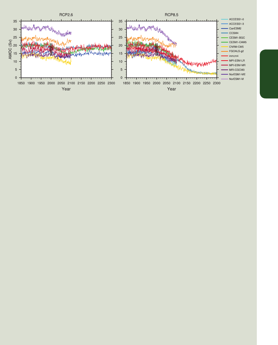
TS
Technical Summary
71
concentrations. The existing modelling studies of permafrost carbon balance under future warming that take into
account at least some of the essential permafrost-related processes do not yield consistent results, beyond the fact
that present-day permafrost will become a net emitter of carbon during the 21st century under plausible future
warming scenarios (low confidence). This also reflects an insufficient understanding of the relevant soil processes
during and after permafrost thaw, including processes leading to stabilization of unfrozen soil carbon, and pre-
cludes any quantitative assessment of the amplitude of irreversible changes in the climate system potentially relat-
ed to permafrost degassing and associated feedbacks. {6.4.7, 12.5.5}
Anthropogenic warming will very likely lead to enhanced CH
4
emissions from both terrestrial and oceanic clathrates.
Deposits of CH
4
clathrates below the sea floor are susceptible to destabilization via ocean warming. However, sea
level rise due to changes in ocean mass enhances clathrate stability in the ocean. While difficult to formally assess,
initial estimates of the 21st century feedback from CH
4
clathrate destabilization are small but not insignificant. It is
very unlikely that CH
4
from clathrates will undergo catastrophic release during the 21st century (high confidence).
On multi-millennial time scales, such CH
4
emissions may provide a positive feedback to anthropogenic warming and
may be irreversible, due to the diffference between release and accumulation time scales. {6.4.7, 12.5.5}
The existence of critical climate change driven dieback thresholds in the Amazonian and other tropical rainforests
purely driven by climate change remains highly uncertain. The possibility of a critical threshold being crossed in
precipitation volume and duration of dry seasons cannot be ruled out. The response of boreal forest to projected
climate change is also highly uncertain, and the existence of critical thresholds cannot at present be ruled out. There
is low confidence in projections of the collapse of large areas of tropical and/or boreal forests. {12.5.5}
Potential Irreversibility of Changes in the Cryosphere
The reversibility of sea ice loss has been directly assessed in sensitivity studies to CO
2
increase and decrease with
Atmosphere–Ocean General Circulation Models (AOGCMs) or Earth System Models (ESMs). None of them show evi-
dence of an irreversible change in Arctic sea ice at any point. By contrast, as a result of the strong coupling between
surface and deep waters in the Southern Ocean, the Antarctic sea ice in some models integrated with ramp-up and
ramp-down atmospheric CO
2
concentration exhibits some hysteresis behaviour. {12.5.5}
At present, both the Greenland and Antarctic ice sheets have a positive surface mass balance (snowfall exceeds
melting), although both are losing mass because ice outflow into the sea exceeds the net surface mass balance. A
positive feedback operates to reduce ice sheet volume and extent when a decrease of the surface elevation of the
ice sheet induces a decreased surface mass balance. This arises generally through increased surface melting, and
therefore applies in the 21st century to Greenland, but not to Antarctica, where surface melting is currently very
small. Surface melting in Antarctica is projected to become important after several centuries under high well-mixed
greenhouse gas radiative forcing scenarios. {4.4, 13.4.4; Boxes 5.2, 13.2}
Abrupt change in ice sheet outflow to the sea may be caused by unstable retreat of the grounding line in regions
where the bedrock is below sea level and slopes downwards towards the interior of the ice sheet. This mainly
(continued on next page)
TFE.5, Figure 1 | Atlantic Meridional Overturning Circulation (AMOC) strength at 30°N (Sv) as a function of year, from 1850 to 2300 as simulated by different Atmo-
sphere–Ocean General Circulation Models in response to scenario RCP2.6 (left) and RCP8.5 (right). The vertical black bar shows the range of AMOC strength measured
at 26°N, from 2004 to 2011 {Figures 3.11, 12.35}
TFE.5 (continued)

TS
Technical Summary
72
applies to West Antarctica, but also to parts of East Antarctica and Greenland. Grounding line retreat can be trig-
gered by ice shelf decay, due to warmer ocean water under ice shelves enhancing submarine ice shelf melt, or melt
water ponds on the surface of the ice shelf promoting ice shelf fracture. Because ice sheet growth is a slow process,
such changes would be irreversible in the definition adopted here. {4.4.5; Box 13.2}
There is high confidence that the volumes of the Greenland and West Antarctic ice sheets were reduced during
periods of the past few million years that were globally warmer than present. Ice sheet model simulations and geo-
logical data suggest that the West Antarctic ice sheet is very sensitive to subsurface ocean warming and imply with
medium confidence a West Antarctic ice sheet retreat if atmospheric CO
2
concentration stays within, or above, the
range of 350–450 ppm for several millennia. {5.8.1, 13.4.4; Box 13.2}
The available evidence indicates that global warming beyond a threshold would lead to the near-complete loss of
the Greenland ice sheet over a millennium or longer, causing a global mean sea level rise of approximately 7 m.
Studies with fixed present-day ice sheet topography indicate that the threshold is greater than 2°C but less than 4°C
(medium confidence) of global mean surface temperature rise above pre-industrial. The one study with a dynamical
ice sheet suggests the threshold is greater than about 1°C (low confidence) global mean warming with respect to
pre-industrial. Considering the present state of scientific uncertainty, a likely range cannot be quantified. The com-
plete loss of the Greenland ice sheet is not inevitable because this would take a millennium or more; if temperatures
decline before the ice sheet has completely vanished, the ice sheet might regrow. However, some part of the mass
loss might be irreversible, depending on the duration and degree of exceedance of the threshold, because the ice
sheet may have multiple steady states, due to its interaction with regional climate. {13.4.3, 13.4.4}
TFE.5 (continued)
TS.4.6 Water Cycle
Since the AR4, new evidence has emerged of a detectable human influ-
ence on several aspects of the water cycle. There is medium confidence
that observed changes in near-surface specific humidity since 1973
contain a detectable anthropogenic component. The anthropogenic
water vapour fingerprint simulated by an ensemble of climate models
has been detected in lower tropospheric moisture content estimates
derived from Special Sensor Microwave/Imager (SSM/I) data covering
the period 1988–2006. An anthropogenic contribution to increases in
tropospheric specific humidity is found with medium confidence. {2.5,
10.3}
Attribution studies of global zonal mean terrestrial precipitation and
Arctic precipitation both find a detectable anthropogenic influence.
Overall there is medium confidence in a significant human influence
on global scale changes in precipitation patterns, including increases
in NH mid-to-high latitudes. Remaining observational and modelling
uncertainties and the large effect of internal variability on observed
precipitation preclude a more confident assessment. {2.5, 7.6, 10.3}
Based on the collected evidence for attributable changes (with varying
levels of confidence and likelihood) in specific humidity, terrestrial pre-
cipitation and ocean surface salinity through its connection to precipi-
tation and evaporation, and from physical understanding of the water
cycle, it is likely that human influence has affected the global water
cycle since 1960. This is a major advance since AR4. {2.4, 2.5, 3.3, 9.4.1,
10.3, 10.4.2; Table 10.1; FAQ 3.2}
TS.4.7 Climate Extremes
Several new attribution studies have found a detectable anthropo-
genic influence in the observed increased frequency of warm days and
nights and decreased frequency of cold days and nights. Since the AR4
and SREX, there is new evidence for detection of human influence on
extremely warm daytime temperature and there is new evidence that
the influence of anthropogenic forcing may be detected separately
from the influence of natural forcing at global scales and in some con-
tinental and sub-continental regions. This strengthens the conclusions
from both AR4 and SREX, and it is now very likely that anthropogenic
forcing has contributed to the observed changes in the frequency and
intensity of daily temperature extremes on the global scale since the
mid-20th century. It is likely that human influence has significantly
increased the probability of occurrence of heat waves in some loca-
tions. See TFE.9 and TFE.9, Table 1 for a summary of the assessment of
extreme weather and climate events. {10.6}
Since the AR4, there is some new limited direct evidence for an anthro-
pogenic influence on extreme precipitation, including a formal detec-
tion and attribution study and indirect evidence that extreme precip-
itation would be expected to have increased given the evidence of
anthropogenic influence on various aspects of the global hydrological
cycle and high confidence that the intensity of extreme precipitation
events will increase with warming, at a rate well exceeding that of the
mean precipitation. In land regions where observational coverage is
sufficient for assessment, there is medium confidence that anthropo-
genic forcing has contributed to a global-scale intensification of heavy
precipitation over the second half of the 20th century. {7.6, 10.6}
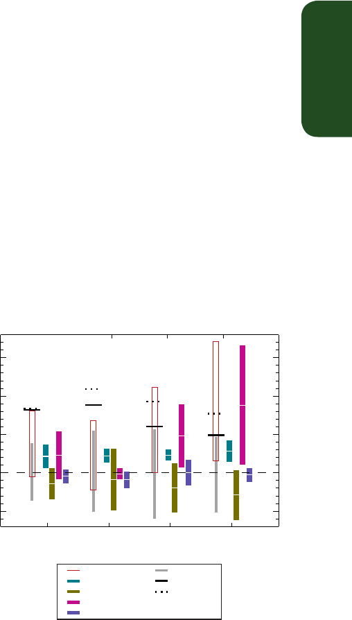
TS
Technical Summary
73
Globally, there is low confidence in attribution of changes in tropical
cyclone activity to human influence. This is due to insufficient observa-
tional evidence, lack of physical understanding of the links between
anthropogenic drivers of climate and tropical cyclone activity, and the
low level of agreement between studies as to the relative importance
of internal variability, and anthropogenic and natural forcings. In the
North Atlantic region there is medium confidence that a reduction in
aerosol forcing over the North Atlantic has contributed at least in part
to the observed increase in tropical cyclone activity there since the
1970s. There remains substantial disagreement on the relative impor-
tance of internal variability, WMGHG forcing and aerosols for this
observed trend. {2.6, 10.6, 14.6}
Although the AR4 concluded that it is more likely than not that anthro-
pogenic influence has contributed to an increased risk of drought in the
second half of the 20th century, an updated assessment of the obser-
vational evidence indicates that the AR4 conclusions regarding global
increasing trends in hydrological droughts since the 1970s are no longer
supported. Owing to the low confidence in observed large-scale trends
in dryness combined with difficulties in distinguishing decadal-scale
variability in drought from long-term climate change, there is now low
confidence in the attribution of changes in drought over global land
since the mid-20th century to human influence. {2.6, 10.6}
TS.4.8 From Global to Regional
Taking a longer term perspective shows the substantial role played by
external forcings in driving climate variability on hemispheric scales in
pre-industrial times (Box TS.5). It is very unlikely that NH temperature
variations from 1400 to 1850 can be explained by internal variability
alone. There is medium confidence that external forcing contributed to
NH temperature variability from 850 to 1400 and that external forcing
contributed to European temperature variations over the last 5 centu-
ries. {5.3.3, 5.5.1, 10.7.2, 10.7.5; Table 10.1}
Changes in atmospheric circulation are important for local climate
change because they could lead to greater or smaller changes in cli-
mate in a particular region than elsewhere. It is likely that human influ-
ence has altered sea level pressure patterns globally. There is medium
confidence that stratospheric ozone depletion has contributed to the
observed poleward shift of the southern Hadley Cell border during aus-
tral summer. It is likely that stratospheric ozone depletion has contrib-
uted to the positive trend in the SAM seen in austral summer since the
mid-20th century which corresponds to sea level pressure reductions
over the high latitudes and increase in the subtropics (Figure TS.11).
{10.3}
The evidence is stronger that observed changes in the climate system
can now be attributed to human activities on global and regional scales
in many components (Figure TS.12). Observational uncertainty has been
explored much more thoroughly than previously, and fingerprints of
human influence have been deduced from a new generation of climate
models. There is improved understanding of ocean changes, including
salinity changes, that are consistent with large scale intensification of
the water cycle predicted by climate models. The changes in near sur-
face temperatures, free atmosphere temperatures, ocean temperatures
and NH snow cover and sea ice extent, when taken together, show not
MAM JJA SON DJF
Season
-0.5
0.0
0.5
1.0
1.5
SAM trend (hPa per decade)
historical
historicalGHG
historicalAer
historicalOz
historicalNat
control
HadSLP2
20CR
Figure TS.11 | Simulated and observed 1951–2011 trends in the Southern Annular
Mode (SAM) index by season. The SAM index is a difference between zonal mean sea
level pressure (SLP) at 40°S and 65°S. The SAM index is defined without normaliza-
tion, so that the magnitudes of simulated and observed trends can be compared. Black
lines show observed trends from the Hadley Centre Sea Level Pressure 2r (HadSLP2r)
data set (solid), and the 20th Century Reanalysis (dotted). Grey bars show 5th to 95th
percentile ranges of control trends, and red boxes show the 5th to 95th percentile
range of trends in historical simulations including anthropogenic and natural forcings.
Coloured bars show ensemble mean trends and their associated 5 to 95% confidence
ranges simulated in response to well-mixed greenhouse gas (light green), aerosol (dark
green), ozone (magenta) and natural forcing changes (blue) in CMIP5 individual-forcing
simulations. {Figure 10.13b}
just global mean changes, but also distinctive regional patterns con-
sistent with the expected fingerprints of change from anthropogenic
forcings and the expected responses from volcanic eruptions (Figure
TS.12). {10.3–10.6, 10.9}
Human influence has been detected in nearly all of the major assessed
components of the climate system (Figure TS.12). Taken together, the
combined evidence increases the overall level of confidence in the
attribution of observed climate change, and reduces the uncertainties
associated with assessment based on a single climate variable. From
this combined evidence it is virtually certain that human influence has
warmed the global climate system. Anthropogenic influence has been
identified in changes in temperature near the surface of the Earth, in
the atmosphere and in the oceans, as well as in changes in the cryo-
sphere, the water cycle and some extremes. There is strong evidence
that excludes solar forcing, volcanoes and internal variability as the
strongest drivers of warming since 1950. {10.9; Table 10.1; FAQ 5.1}
Over every continent except Antarctica, anthropogenic influence has
likely made a substantial contribution to surface temperature increas-
es since the mid-20th century (Figure TS.12). It is likely that there has
been a significant anthropogenic contribution to the very substantial
warming in Arctic land surface temperatures over the past 50 years.
For Antarctica large observational uncertainties result in low confidence
that anthropogenic influence has contributed to observed warming
averaged over available stations. Detection and attribution at regional
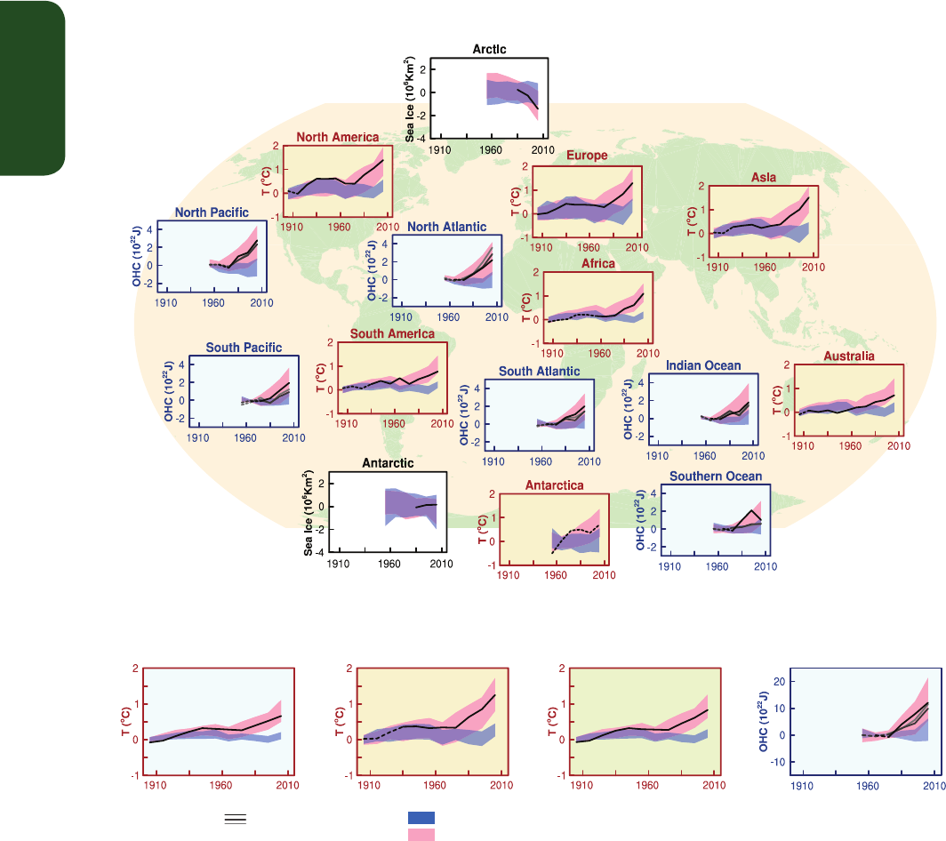
TS
Technical Summary
74
scales is complicated by the greater role played by dynamical factors
(circulation changes), a greater range of forcings that may be regionally
important, and the greater difficulty of modelling relevant processes at
regional scales. Nevertheless, human influence has likely contributed to
temperature increases in many sub-continental regions. {10.3; Box 5.1}
The coherence of observed changes with simulations of anthropogenic
and natural forcing in the physical system is remarkable (Figure TS.12),
particularly for temperature-related variables. Surface temperature and
Observations
Models using only natural forcings
Models using both natural and anthropogenic forcings
Global averages
Land surface Land and ocean surface Ocean heat contentOcean surface
Figure TS.12 | Comparison of observed and simulated change in the climate system, at regional scales (top panels) and global scales (bottom four panels). Brown panels are land
surface temperature time series, blue panels are ocean heat content time series and white panels are sea ice time series (decadal averages). Each panel shows observations (black
or black and shades of grey), and the 5 to 95% range of the simulated response to natural forcings (blue shading) and natural and anthropogenic forcings (pink shading), together
with the corresponding ensemble means (dark blue and dark red respectively). The observed surface temperature is from the Hadley Centre/Climatic Research Unit gridded surface
temperature data set 4 (HadCRUT4). Three observed records of ocean heat content (OHC) are shown. Sea ice anomalies (rather than absolute values) are plotted and based on
models in Figure 10.16. The observations lines are either solid or dashed and indicate the quality of the observations and estimates. For land and ocean surface temperatures panels
and precipitation panels, solid observation lines indicate where spatial coverage of areas being examined is above 50% coverage and dashed observation lines where coverage is
below 50%. For example, data coverage of Antarctica never goes above 50% of the land area of the continent. For ocean heat content and sea ice panels the solid observations line
is where the coverage of data is good and higher in quality, and the dashed line is where the data coverage is only adequate. This figure is based on Figure 10.21 except presented
as decadal averages rather than yearly averages. Further detail regarding the related Figure SPM.6 is given in the TS Supplementary Material. {Figure 10.21}
ocean heat content show emerging anthropogenic and natural signals
in both records, and a clear separation from the alternative hypothesis
of just natural variations. These signals do not appear just in the global
means, but also appear at regional scales on continents and in ocean
basins in each of these variables. Sea ice extent emerges clearly from
the range of internal variability for the Arctic. At sub-continental scales
human influence is likely to have substantially increased the probabil-
ity of occurrence of heat waves in some locations. {Table 10.1}

TS
Technical Summary
75
Box TS.4 | Model Evaluation
Climate models have continued to be improved since the AR4, and many models have been extended into Earth System Models (ESMs)
by including the representation of biogeochemical cycles important to climate change. Box TS.4, Figure 1 provides a partial overview of
model capabilities as assessed in this report, including improvements or lack thereof relative to models that were assessed in the AR4
or that were available at the time of the AR4. {9.1, 9.8.1; Box 9.1}
The ability of climate models to simulate surface temperature has improved in many, though not all, important aspects relative to the
generation of models assessed in the AR4. There continues to be very high confidence that models reproduce the observed large-scale
time-mean surface temperature patterns (pattern correlation of about 0.99), although systematic errors of several degrees Celsius are
found in some regions. There is high confidence that on the regional scale (sub-continental and smaller), time-mean surface tempera-
ture is better simulated than at the time of the AR4; however, confidence in model capability is lower than for the large scale. Models
are able to reproduce the magnitude of the observed global mean or northern-hemisphere-mean temperature variability on interannual
to centennial time scales. Models are also able to reproduce the large-scale patterns of temperature during the Last Glacial Maximum
indicating an ability to simulate a climate state much different from the present (see also Box TS.5). {9.4.1, 9.6.1}
There is very high confidence that models reproduce the general features of the global and annual mean surface temperature changes
over the historical period, including the warming in the second half of the 20th century and the cooling immediately following large
volcanic eruptions. Most simulations of the historical period do not reproduce the observed reduction in global mean surface warming
trend over the last 10 to 15 years (see Box TS.3). There is medium confidence that the trend difference between models and observa-
tions during 1998–2012 is to a substantial degree caused by internal variability, with possible contributions from forcing inadequacies
in models and some models overestimating the response to increasing greenhouse gas forcing. Most, though not all, models overesti-
mate the observed warming trend in the tropical troposphere over the last 30 years, and tend to underestimate the long-term lower-
stratospheric cooling trend. {9.4.1; Box 9.2}
The simulation of large-scale patterns of precipitation has improved somewhat since the AR4, although models continue to perform
less well for precipitation than for surface temperature. The spatial pattern correlation between modelled and observed annual mean
precipitation has increased from 0.77 for models available at the time of the AR4 to 0.82 for current models. At regional scales, precipi-
tation is not simulated as well, and the assessment remains difficult owing to observational uncertainties. {9.4.1, 9.6.1}
Many models are able to reproduce the observed changes in upper-ocean heat content from 1961 to 2005. The time series of the multi-
model mean falls within the range of the available observational estimates for most of the period. {9.4.2}
There is robust evidence that the downward trend in Arctic summer sea ice extent is better simulated than at the time of the AR4. About
one quarter of the models show a trend as strong as, or stronger, than the trend in observations over the satellite era 1979–2012.
Most models simulate a small decreasing trend in Antarctic sea ice extent, albeit with large inter-model spread, in contrast to the small
increasing trend in observations. {9.4.3}
There has been substantial progress since the AR4 in the assessment of model simulations of extreme events. Changes in the frequency
of extreme warm and cold days and nights over the second half of the 20th century are consistent between models and observations,
with the ensemble mean global mean time series generally falling within the range of observational estimates. The majority of models
underestimate the sensitivity of extreme precipitation to temperature variability or trends, especially in the tropics. {9.5.4}
In the majority of the models that include an interactive carbon cycle, the simulated global land and ocean carbon sinks over the latter
part of the 20th century fall within the range of observational estimates. However, models systematically underestimate the NH land
sink implied by atmospheric inversion techniques. {9.4.5}
Regional downscaling methods provide climate information at the smaller scales needed for many climate impact studies. There is high
confidence that downscaling adds value both in regions with highly variable topography and for various small-scale phenomena. {9.6.4}
The model spread in equilibrium climate sensitivity ranges from 2.1°C to 4.7°C and is very similar to the assessment in the AR4. There
is very high confidence that the primary factor contributing to the spread in equilibrium climate sensitivity continues to be the cloud
feedback. This applies to both the modern climate and the last glacial maximum. There is likewise very high confidence that, consis-
tent with observations, models show a strong positive correlation between tropospheric temperature and water vapour on regional
to global scales, implying a positive water vapour feedback in both models and observations. {5.3.3, 9.4.1, 9.7} (continued on next page)

TS
Technical Summary
76
Box TS.4 (continued)
Climate models are based on physical principles, and they reproduce many important elements of observed climate. Both aspects
contribute to our confidence in the models’ suitability for their application in detection and attribution studies (see Chapter 10) and for
quantitative future predictions and projections (see Chapters 11 to 14). There is increasing evidence that some elements of observed
variability or trends are well correlated with inter-model differences in model projections for quantities such as Arctic summer sea ice
trends, the snow–albedo feedback, and the carbon loss from tropical land. However, there is still no universal strategy for transferring
a model’s past performance to a relative weight of this model in a multi-model-ensemble mean of climate projections. {9.8.3}
Box TS.4, Figure1 | Summary of how well the current-generation climate models simulate important features of the climate of the 20th century. Confidence in the
assessment increases towards the right as suggested by the increasing strength of shading. Model quality increases from bottom to top. The colour coding indicates
improvements from the models available at the time of the AR4 to the current assessment. There have been a number of improvements since the AR4, and some some
modelled quantities are not better simulated. The major climate quantities are listed in this summary and none shows degradation. The assessment is based mostly on
the multi-model mean, not excluding that deviations for individual models could exist. Assessed model quality is simplified for representation in this figure; details of
each assessment are found in Chapter 9. {9.8.1; Figure 9.44}
The figure highlights the following key features, with the sections that back up the assessment added in brackets:
(a) Trends in:
AntSIE Antarctic sea ice extent {9.4.3}
ArctSIE Arctic sea ice extent {9.4.3}
fgCO2 Global ocean carbon sink {9.4.5}
LST Lower-stratospheric temperature {9.4.1.}
NBP Global land carbon sink {9.4.5}
OHC Global ocean heat content {9.4.2}
TotalO3 Total-column ozone {9.4.1}
TAS Surface air temperature {9.4.1}
TTT Tropical tropospheric temperature {9.4.1}
(b) Extremes:
Droughts Droughts {9.5.4}
Hurric-hr Year-to-year count of Atlantic hurricanes in high-resolution AGCMs {9.5.4}
PR_ext Global distribution of precipitation extremes {9.5.4}
PR_ext-hr Global distribution of precipitation extremes in high-resolution AGCMs {9.5.4}
PR_ext-t Global trends in precipitation extremes {9.5.4}
TAS_ext Global distributions of surface air temperature extremes {9.5.4}
TAS_ext-t Global trends in surface air temperature extremes {9.5.4}
TC Tropical cyclone tracks and intensity {9.5.4}
TC-hr Tropical cyclone tracks and intensity in high-resolution AGCMs {9.5.4}
Very low Low Medium High Very high
Low Medium High
(a) Trends
OHC
TotalO3
TTT
LST
ArctSIE
AntSIE
TAS
Model performance
Confidence in assessment
NBP
fgCO2
Very low Low Medium High Very high
Low Medium High
(b) Extremes
TAS_ext
Doughts
TAS_ext -t
PR_ext -t
PR_ext
PR_ext -hr
TC-hr
Hurric -hr
Model performance
Confidence in assessment
TC
Degradation since the AR4
No change since the AR4
Improvement since the AR4
Not assessed in the AR4

TS
Technical Summary
77
Box TS.5 | Paleoclimate
Reconstructions from paleoclimate archives allow current changes in atmospheric composition, sea level and climate (including extreme
events such as droughts and floods), as well as future projections, to be placed in a broader perspective of past climate variability (see
Section TS.2). {5.2–5.6, 6.2, 10.7}
Past climate information also documents the behaviour of slow components of the climate system including the carbon cycle, ice sheets
and the deep ocean for which instrumental records are short compared to their characteristic time scales of responses to perturba-
tions, thus informing on mechanisms of abrupt and irreversible changes. Together with the knowledge of past external climate forcings,
syntheses of paleoclimate data have documented polar amplification, characterized by enhanced temperature changes in the Arctic
compared to the global mean, in response to high or low CO
2
concentrations. {5.2.1, 5.2.2, 5.6, 5.7, 5.8, 6.2, 8.4.2, 13.2.1, 13.4; Boxes
5.1, 5.2}
Since AR4, the inclusion of paleoclimate simulations in the PMIP3 (Paleoclimate Modelling Intercomparison Project)/CMIP5 framework
has enabled paleoclimate information to be more closely linked with future climate projections. Paleoclimate information for the mid-
Holocene (6 ka), the Last Glacial Maximum (approximately 21 ka), and last millennium has been used to test the ability of models to
simulate realistically the magnitude and large-scale patterns of past changes. Combining information from paleoclimate simulations
and reconstructions enables to quantify the response of the climate system to radiative perturbations, constraints to be placed on the
range of equilibrium climate sensitivity, and past patterns of internal climate variability to be documented on inter-annual to multi-
centennial scales. {5.3.1–5.3.5, 5.4, 5.5.1, 9.4.1, 9.4.2, 9.5.3, 9.7.2, 10.7.2, 14.1.2}
Box TS.5, Figure 1 illustrates the comparison between the last millennium Paleoclimate Modelling Intercomparison Project Phase 3
(PMIP3)/CMIP5 simulations and reconstructions, together with the associated solar, volcanic and WMGHG RFs. For average annual NH
temperatures, the period 1983–2012 was very likely the warmest 30-year period of the last 800 years (high confidence) and likely the
warmest 30-year period of the last 1400 years (medium confidence). This is supported by comparison of instrumental temperatures
with multiple reconstructions from a variety of proxy data and statistical methods, and is consistent with AR4. In response to solar,
volcanic and anthropogenic radiative changes, climate models simulate multi-decadal temperature changes in the last 1200 years in
the NH that are generally consistent in magnitude and timing with reconstructions, within their uncertainty ranges. Continental-scale
temperature reconstructions show, with high confidence, multi-decadal periods during the Medieval Climate Anomaly (about 950 to
1250) that were in some regions as warm as the mid-20th century and in others as warm as in the late 20th century. With high confi-
dence, these regional warm periods were not as synchronous across regions as the warming since the mid-20th century. Based on the
comparison between reconstructions and simulations, there is high confidence that not only external orbital, solar and volcanic forcing
but also internal variability contributed substantially to the spatial pattern and timing of surface temperature changes between the
Medieval Climate Anomaly and the Little Ice Age (about 1450 to 1850). However, there is only very low confidence in quantitative esti-
mates of their relative contributions. It is very unlikely that NH temperature variations from 1400 to 1850 can be explained by internal
variability alone. There is medium confidence that external forcing contributed to Northern Hemispheric temperature variability from
850 to 1400 and that external forcing contributed to European temperature variations over the last 5 centuries. {5.3.5, 5.5.1, 10.7.2,
10.7.5; Table 10.1} (continued on next page)

TS
Technical Summary
78
Time (Year CE)
VolcanicWell mixed GHGs
1000 1200 1400 1600 1800
2000
0.0
-0.5
0.5
1.0
1.5
2.0
2.5
TSI
-0.3
-0.2
0.0
-0.1
0.1
0
-5
-10
-15
-20
1000 1200 1400 1600 1800 2000
Time (Year CE)
-0.5
0.0
0.5
1.0
Temp. anomaly wrt 1500 - 1850 (°C)
−2
−1.5
−1
−0.5
0
0.5
1
1.5
2
−2
−1.5
−1
−0.5
0
0.5
1
1.5
(f) Asia JJA
Temp. anomaly wrt 1881−1980 (°C)
Temp. anomaly wrt 1500−1850 (°C)
1000 1200 1400 1600 1800 2000
Time (Year CE)
Europe
Asia
Arctic
North
America
(a) Radiative forcing (W m
-2
)
(b) Reconstructed (grey) and simulated (red) NH temperature
−2
−1.5
−1
−0.5
0
0.5
1
1.5
2
−2
−1.5
−1
−0.5
0
0.5
1
Temp. anomaly wrt 1500−1850 (°C)
Temp. anomaly wrt 1881−1980 (°C)
1000 1200 1400 1600 1800 2000
Time (Year CE)
(c) Arctic ANN
−2
−1.5
−1
−0.5
0
0.5
1
1.5
2
−2
−1.5
−1
−0.5
0
0.5
1
1.5
(e) Europe JJA
Temp. anomaly wrt 1881−1980 (°C)
Temp. anomaly wrt 1500−1850 (°C)
1000 1200 1400 1600 1800 2000
Time (Year CE)
−2
−1.5
−1
−0.5
0
0.5
1
1.5
2
−2
−1.5
−1
−0.5
0
0.5
1
1.5
(d) North America ANN
Temp. anomaly wrt 1881−1980 (°C)
Temp. anomaly wrt 1500−1850 (°C)
1000 1200 1400 1600 1800 2000
Time (Year CE)
Box TS.5 (continued)
Box TS.5, Figure 1 | Last-millennium simulations and reconstructions. (a) 850–2000 PMIP3/CMIP5 radiative forcing due to volcanic, solar and well-mixed green-
house gases. Different colours illustrate the two existing data sets for volcanic forcing and four estimates of solar forcing. For solar forcing, solid (dashed) lines stand
for reconstruction variants in which background changes in irradiance are (not) considered; (b) 850–2000 PMIP3/CMIP5 simulated (red) and reconstructed (shading)
Northern Hemisphere (NH) temperature changes. The thick red line depicts the multi-model mean while the thin red lines show the multi-model 90% range. The
overlap of reconstructed temperatures is shown by grey shading; all data are expressed as anomalies from their 1500–1850 mean and smoothed with a 30-year filter.
Note that some reconstructions represent a smaller spatial domain than the full NH or a specific season, while annual temperatures for the full NH mean are shown
for the simulations. (c), (d), (e) and (f) Arctic and North America annual mean temperature, and Europe and Asia June, July and August (JJA) temperature, from 950 to
2000 from reconstructions (black line), and PMIP3/CMIP5 simulations (thick red, multi-model mean; thin red, 90% multi-model range). All red curves are expressed
as anomalies from their 1500–1850 mean and smoothed with a 30-year filter. The shaded envelope depicts the uncertainties from each reconstruction (Arctic: 90%
confidence bands, North American: ±2 standard deviation. Asia: ±2 root mean square error. Europe: 95% confidence bands). For comparison with instrumental record,
the Climatic Research Unit land station Temperature (CRUTEM4) data set is shown (yellow line). These instrumental data are not necessarily those used in calibration
of the reconstrctions, and thus may show greater or lesser correspondence with the reconstructions than the instrumental data actually used for calibration; cutoff
timing may also lead to end effects for smoothed data shown. All lines are smoothed by applying a 30-year moving average. Map shows the individual regions for each
reconstruction. {5.3.5; Table 5.A.1; Figures 5.1, 5.8, 5.12}

TS
Technical Summary
79
TS.5 Projections of Global and Regional
Climate Change
TS.5.1 Introduction
Projections of changes in the climate system are made using a hierar-
chy of climate models ranging from simple climate models, to models
of intermediate complexity, to comprehensive climate models, and
Earth System Models (ESMs). These models simulate changes based
on a set of scenarios of anthropogenic forcings. A new set of scenarios,
the Representative Concentration Pathways (RCPs), was used for the
new climate model simulations carried out under the framework of
the Coupled Model Intercomparison Project Phase 5 (CMIP5) of the
World Climate Research Programme. A large number of comprehensive
climate models and ESMs have participated in CMIP5, whose results
form the core of the climate system projections.
This section summarizes the assessment of these climate change pro-
jections. First, future forcing and scenarios are presented. The following
subsections then address various aspects of projections of global and
regional climate change, including near-term (up to about mid-century)
and long-term (end of the 21st century) projections in the atmosphere,
ocean and cryosphere; projections of carbon and other biogeochemical
cycles; projections in sea level change; and finally changes to climate
phenomena and other aspects of regional climate over the 21st cen-
tury. Projected changes are given relative to the 1986–2005 average
unless indicated otherwise. Projections of climate change on longer
term and information on climate stabilization and targets are provided
in TFE.8. Methods to counter climate change, termed geoengineering,
have been proposed and an overview is provided in Box TS.7. {11.3,
12.3–12.5, 13.5–13.7, 14.1–14.6, Annex I}
TS.5.2 Future Forcing and Scenarios
In this assessment report a series of new RCPs are used that largely
replace the IPCC Special Report on Emission Scenarios (SRES) scenarios
(see Box TS.6 and Annex II for Climate System Scenario Tables). They
produce a range of responses from ongoing warming, to approximately
stabilized forcing, to a stringent mitigation scenario (RCP2.6) that sta-
bilizes and then slowly reduces the RF after mid-21st century. In con-
trast to the AR4, the climate change from the RCP scenarios in the AR5
is framed as a combination of adaptation and mitigation. Mitigation
actions starting now in the various RCP scenarios do not produce dis-
cernibly different climate change outcomes for the next 30 years or
so, whereas long-term climate change after mid-century is appreciably
different across the RCPs. {Box 1.1}
Box TS.6 | The New Representative Concentration Pathway Scenarios and Coupled Model Intercomparison
Project Phase 5 Models
Future anthropogenic emissions of GHGs, aerosol particles and other forcing agents such as land use change are dependent on socio-
economic factors, and may be affected by global geopolitical agreements to control those emissions to achieve mitigation. AR4 made
extensive use of the SRES scenarios that do not include additional climate initiatives, which means that no scenarios were available
that explicitly assume implementation of the United Nations Framework Convention on Climate Change (UNFCCC) or the emissions
targets of the Kyoto Protocol. However, GHG emissions are directly affected by non-climate change policies designed for a wide range
of other purposes. The SRES scenarios were developed using a sequential approach, that is, socioeconomic factors fed into emissions
scenarios, which were then used in simple climate models to determine concentrations of GHGs, and other agents required to drive the
more complex AOGCMs. In this report, outcomes of climate simulations that use new scenarios (some of which include implied policy
actions to achieve mitigation) referred to as RCPs are assessed. These RCPs represent a larger set of mitigation scenarios and were
selected to have different targets in terms of radiative forcing at 2100 (about 2.6, 4.5, 6.0 and 8.5 W m
–2
; Figure TS.15). The scenarios
should be considered plausible and illustrative, and do not have probabilities attached to them. {12.3.1; Box 1.1}
The RCPs were developed using Integrated Assessment Models (IAMs) that typically include economic, demographic, energy, and
simple climate components. The emission scenarios they produce are then run through a simple model to produce time series of GHG
concentrations that can be run in AOGCMs. The emission time series from the RCPs can then be used directly in ESMs that include
interactive biogeochemistry (at least a land and ocean carbon cycle). {12.3.1; Box 1.1}
The CMIP5 multi-model experiment (coordinated through the World Climate Research Programme) presents an unprecedented level of
information on which to base assessments of climate variability and change. CMIP5 includes new ESMs in addition to AOGCMs, new
model experiments and more diagnostic output. CMIP5 is much more comprehensive than the preceding CMIP3 multi-model experi-
ment that was available at the time of the IPCC AR4. CMIP5 has more than twice as many models, many more experiments (that also
include experiments to address understanding of the responses in the future climate change scenario runs), and nearly 2 × 10
15
bytes
of data (as compared to over 30 × 10
12
bytes of data in CMIP3). A larger number of forcing agents are treated more completely in the
CMIP5 models, with respect to aerosols and land use particularly. Black carbon aerosol is now a commonly included forcing agent.
Considering CO
2
, both ‘concentrations-driven’ projections and ‘emissions-driven’ projections are assessed from CMIP5. These allow
quantification of the physical response uncertainties as well as climate–carbon cycle interactions. {1.5.2}
(continued on next page)
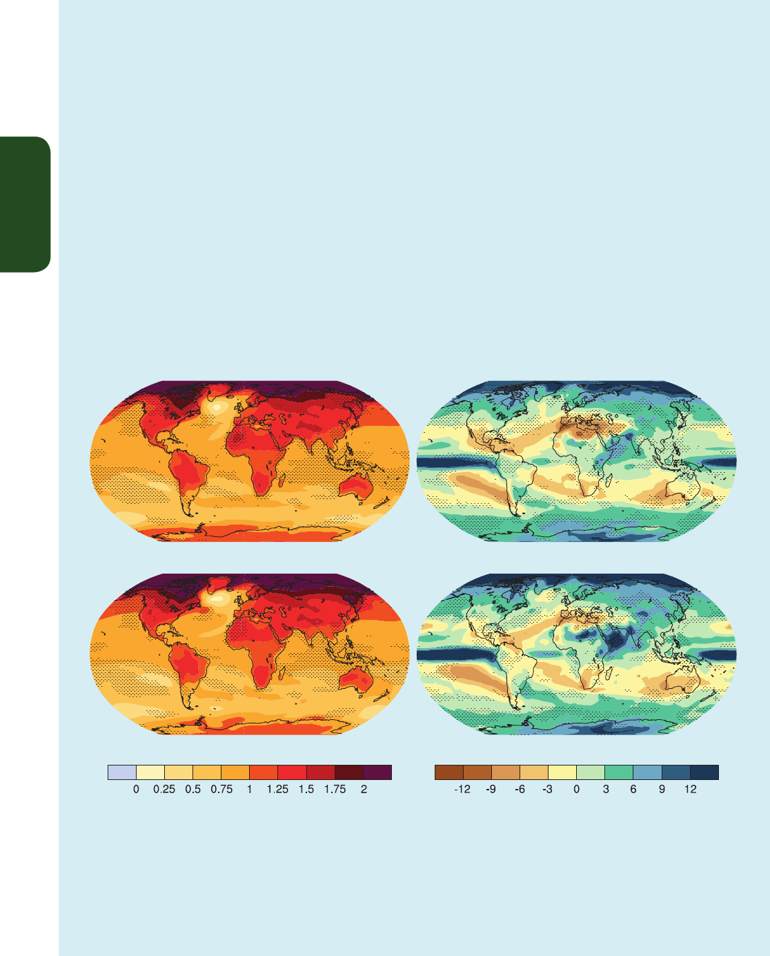
TS
Technical Summary
80
Box TS.6 (continued)
The assessment of the mean values and ranges of global mean temperature changes in AR4 would not have been substantially dif-
ferent if the CMIP5 models had been used in that report. The differences in global temperature projections can largely be attributed
to the different scenarios. The global mean temperature response simulated by CMIP3 and CMIP5 models is very similar, both in the
mean and the model range, transiently and in equilibrium. The range of temperature change across all scenarios is wider because the
RCPs include a strong mitigation scenario (RCP2.6) that had no equivalent among the SRES scenarios used in CMIP3. For each scenario,
the 5 to 95% range of the CMIP5 projections is obtained by approximating the CMIP5 distributions by a normal distribution with
same mean and standard deviation and assessed as being likely for projections of global temperature change for the end of the 21st
century. Probabilistic projections with simpler models calibrated to span the range of equilibrium climate sensitivity assessed by the
AR4 provide uncertainty ranges that are consistent with those from CMIP5. In AR4 the uncertainties in global temperature projections
were found to be approximately constant when expressed as a fraction of the model mean warming (constant fractional uncertainty).
For the higher RCPs, the uncertainty is now estimated to be smaller than with the AR4 method for long-term climate change, because
the carbon cycle–climate feedbacks are not relevant for the concentration-driven RCP projections (in contrast, the assessed projection
uncertainties of global temperature in AR4 did account of carbon cycle–climate feedbacks, even though these were not part of the
CMIP3 models). When forced with RCP8.5, CO
2
emissions, as opposed to the RCP8.5 CO
2
concentrations, CMIP5 ESMs with interactive
carbon cycle simulate, on average, a 50 (–140 to +210) ppm (CMIP5 model spread) larger atmospheric CO
2
concentration and 0.2°C
larger global surface temperature increase by 2100. For the low RCPs the fractional uncertainty is larger because internal variability and
non-CO
2
forcings make a larger relative contribution to the total uncertainty. {12.4.1, 12.4.8, 12.4.9} (continued on next page)
Temperature scaled by global T (°C per °C)
CMIP3 : 2080-2099
Precipitation scaled by global T (% per °C)
CMIP3 : 2080-2099
CMIP5 : 2081-2100
CMIP5 : 2081-2100
(°C per °C global mean change) (% per °C global mean change)
Box TS.6, Figure 1 | Patterns of temperature (left column) and percent precipitation change (right column) for the CMIP3 models average (first row) and CMIP5
models average (second row), scaled by the corresponding global average temperature changes. The patterns are computed in both cases by taking the difference
between the averages over the last 20 years of the 21st century experiments (2080–2099 for CMIP3 and 2081–2100 for CMIP5) and the last 20 years of the historic
experiments (1980–1999 for CMIP3, 1986–2005 for CMIP5) and rescaling each difference by the corresponding change in global average temperature. This is done
first for each individual model, then the results are averaged across models. Stippling indicates a measure of significance of the difference between the two correspond-
ing patterns obtained by a bootstrap exercise. Two subsets of the pooled set of CMIP3 and CMIP5 ensemble members of the same size as the original ensembles, but
without distinguishing CMIP3 from CMIP5 members, were randomly sampled 500 times. For each random sample the corresponding patterns and their difference are
computed, then the true difference is compared, grid-point by grid-point, to the distribution of the bootstrapped differences, and only grid-points at which the value of
the difference falls in the tails of the bootstrapped distribution (less than the 2.5th percentiles or the 97.5th percentiles) are stippled. {Figure 12.41}

TS
Technical Summary
81
The range in anthropogenic aerosol emissions across all scenarios has
a larger impact on near-term climate projections than the correspond-
ing range in long-lived GHGs, particularly on regional scales and for
hydrological cycle variables. The RCP scenarios do not span the range
of future aerosol emissions found in the SRES and alternative scenarios
(Box TS.6). {11.3.1, 11.3.6}
If rapid reductions in sulphate aerosol are undertaken for improving air
quality or as part of decreasing fossil-fuel CO2 emissions, then there is
medium confidence that this could lead to rapid near-term warming.
There is evidence that accompanying controls on CH
4
emissions would
offset some of this sulphate-induced warming, although the cool-
ing from CH
4
mitigation will emerge more slowly than the warming
from sulphate mitigation due to the different time scales over which
atmospheric concentrations of these substances decrease in response
to decreases in emissions. Although removal of black carbon aerosol
could also counter warming associated with sulphate removal, uncer-
tainties are too large to constrain the net sign of the global tempera-
ture response to black carbon emission reductions, which depends on
reduction of co-emitted (reflective) aerosols and on aerosol indirect
effects. {11.3.6}
Including uncertainties in projecting the chemically reactive GHGs CH
4
and N
2
O from RCP emissions gives a range in abundance pathways
that is likely 30% larger than the range in RCP concentrations used to
force the CMIP5 climate models. Including uncertainties in emission
estimates from agricultural, forest and land use sources, in atmospheric
lifetimes, and in chemical feedbacks, results in a much wider range of
abundances for N
2
O, CH
4
and HFCs and their RF. In the case of CH
4
,
by year 2100 the likely range of RCP8.5 CH
4
abundance extends 520
ppb above the single-valued RCP8.5 CH
4
abundance, and RCP2.6 CH
4
extends 230 ppb below RCP2.6 CH
4
. {11.3.5}
There is very low confidence in projections of natural forcing. Major
volcanic eruptions cause a negative RF up to several watts per square
metre, with a typical lifetime of one year, but the possible occurrence
and timing of future eruptions is unknown. Except for the 11-year solar
cycle, changes in the total solar irradiance are uncertain. Except where
explicitly indicated, future volcanic eruptions and changes in total solar
irradiance additional to a repeating 11-year solar cycle are not included
in the projections of near- and long-term climate assessed. {8, 11.3.6}
TS.5.3 Quantification of Climate System Response
Estimates of the equilibrium climate sensitivity (ECS) based on
observed climate change, climate models and feedback analysis, as
well as paleoclimate evidence indicate that ECS is positive, likely in
the range 1.5°C to 4.5°C with high confidence, extremely unlikely less
than 1°C (high confidence) and very unlikely greater than 6°C (medium
confidence). Earth system sensitivity over millennia time scales includ-
ing long-term feedbacks not typically included in models could be sig-
nificantly higher than ECS (see TFE.6 for further details). {5.3.1, 10.8;
Box 12.2}
With high confidence the transient climate response (TCR) is positive,
likely in the range 1°C to 2.5°C and extremely unlikely greater than
3°C, based on observed climate change and climate models (see TFE.6
for further details). {10.8; Box 12.2}
The ratio of GMST change to total cumulative anthropogenic carbon
emissions is relatively constant and independent of the scenario, but is
model dependent, as it is a function of the model cumulative airborne
fraction of carbon and the transient climate response. For any given
temperature target, higher emissions in earlier decades therefore imply
lower emissions by about the same amount later on. The transient cli-
mate response to cumulative carbon emission (TCRE) is likely between
0.8°C to 2.5°C per 1000 PgC (high confidence), for cumulative carbon
emissions less than about 2000 PgC until the time at which tempera-
tures peak (see TFE.8 for further details). {10.8, 12.5.4; Box 12.2}
Box TS.6 (continued)
There is overall consistency between the projections of temperature and precipitation based on CMIP3 and CMIP5, both for large-scale
patterns and magnitudes of change (Box TS.6, Figure 1). Model agreement and confidence in projections depends on the variable and
on spatial and temporal averaging, with better agreement for larger scales. Confidence is higher for temperature than for those quan-
tities related to the water cycle or atmospheric circulation. Improved methods to quantify and display model robustness have been
developed to indicate where lack of agreement across models on local trends is a result of internal variability, rather than models actu-
ally disagreeing on their forced response. Understanding of the sources and means of characterizing uncertainties in long-term large
scale projections of climate change has not changed significantly since AR4, but new experiments and studies have continued to work
towards a more complete and rigorous characterization. {9.7.3, 12.2, 12.4.1, 12.4.4, 12.4.5, 12.4.9; Box 12.1}
The well-established stability of geographical patterns of temperature and precipitation change during a transient experiment remains
valid in the CMIP5 models (Box TS.6, Figure 1). Patterns are similar over time and across scenarios and to first order can be scaled by
the global mean temperature change. There remain limitations to the validity of this technique when it is applied to strong mitigation
scenarios, to scenarios where localized forcings (e.g., aerosols) are significant and vary in time and for variables other than average
seasonal mean temperature and precipitation. {12.4.2}

TS
Technical Summary
82
Thematic Focus Elements
TFE.6 | Climate Sensitivity and Feedbacks
The description of climate change as a response to a forcing that is amplified by feedbacks goes back many decades.
The concepts of radiative forcing (RF) and climate feedbacks continue to be refined, and limitations are now better
understood; for instance, feedbacks may be much faster than the surface warming, feedbacks depend on the type of
forcing agent (e.g., greenhouse gas (GHG) vs. solar forcing), or may have intrinsic time scales (associated mainly with
vegetation change and ice sheets) of several centuries to millennia. The analysis of physical feedbacks in models and
from observations remains a powerful framework that provides constraints on transient future warming for differ-
ent scenarios, on climate sensitivity and, combined with estimates of carbon cycle feedbacks (see TFE.5), determines
the GHG emissions that are compatible with climate stabilization or targets (see TFE.8). {7.1, 9.7.2, 12.5.3; Box 12.2}
The water vapour/lapse rate, albedo and cloud feedbacks are the principal determinants of equilibrium climate
sensitivity. All of these feedbacks are assessed to be positive, but with different levels of likelihood assigned rang-
ing from likely to extremely likely. Therefore, there is high confidence that the net feedback is positive and the
black body response of the climate to a forcing will therefore be amplified. Cloud feedbacks continue to be the
largest uncertainty. The net feedback from water vapour and lapse rate changes together is extremely likely posi-
tive and approximately doubles the black body response. The mean value and spread of these two processes in
climate models are essentially unchanged from the IPCC Fourth Assessment Report (AR4), but are now supported
by stronger observational evidence and better process understanding of what determines relative humidity dis-
tributions. Clouds respond to climate forcing mechanisms in multiple ways and individual cloud feedbacks can be
positive or negative. Key issues include the representation of both deep and shallow cumulus convection, micro-
physical processes in ice clouds and partial cloudiness that results from small-scale variations of cloud-producing and
cloud-dissipating processes. New approaches to diagnosing cloud feedback in General Circulation Models (GCMs)
have clarified robust cloud responses, while continuing to implicate low cloud cover as the most important source
of intermodel spread in simulated cloud feedbacks. The net radiative feedback due to all cloud types is likely posi-
tive. This conclusion is reached by considering a plausible range for unknown contributions by processes yet to be
accounted for, in addition to those occurring in current climate models. Observations alone do not currently pro-
vide a robust, direct constraint, but multiple lines of evidence now indicate positive feedback contributions from
changes in both the height of high clouds and the horizontal distribution of clouds. The additional feedback from
low cloud amount is also positive in most climate models, but that result is not well understood, nor effectively
constrained by observations, so confidence in it is low. {7.2.4–7.2.6, 9.7.2}
The representation of aerosol–cloud processes in climate models continues to be a challenge. Aerosol and cloud
variability at scales significantly smaller than those resolved in climate models, and the subtle responses of clouds to
aerosol at those scales, mean that, for the foreseeable future, climate models will continue to rely on parameteriza-
tions of aerosol–cloud interactions or other methods that represent subgrid variability. This implies large uncertain-
ties for estimates of the forcings associated with aerosol–cloud interactions. {7.4, 7.5.3, 7.5.4}
Equilibrium climate sensitivity (ECS) and transient climate response (TCR) are useful metrics summarising the global
climate system’s temperature response to an externally imposed RF. ECS is defined as the equilibrium change in
annual mean global mean surface temperature (GMST) following a doubling of the atmospheric carbon dioxide
(CO
2
) concentration, while TCR is defined as the annual mean GMST change at the time of CO
2
doubling following a
linear increase in CO
2
forcing over a period of 70 years (see Glossary). Both metrics have a broader application than
these definitions imply: ECS determines the eventual warming in response to stabilisation of atmospheric composi-
tion on multi-century time scales, while TCR determines the warming expected at a given time following any steady
increase in forcing over a 50- to 100-year time scale. {Box 12.2; 12.5.3}
ECS and TCR can be estimated from various lines of evidence (TFE.6, Figures 1 and 2). The estimates can be based on
the values of ECS and TCR diagnosed from climate models, or they can be constrained by analysis of feedbacks in
climate models, patterns of mean climate and variability in models compared to observations, temperature fluctua-
tions as reconstructed from paleoclimate archives, observed and modelled short term perturbations of the energy
balance like those caused by volcanic eruptions, and the observed surface and ocean temperature trends since pre-
industrial. For many applications, the limitations of the forcing-feedback analysis framework and the dependence
of feedbacks on time scales and the climate state must be kept in mind. {5.3.1, 5.3.3, 9.7.1–9.7.3, 10.8.1, 10.8.2,
12.5.3; Box 5.2; Table 9.5} (continued on next page)
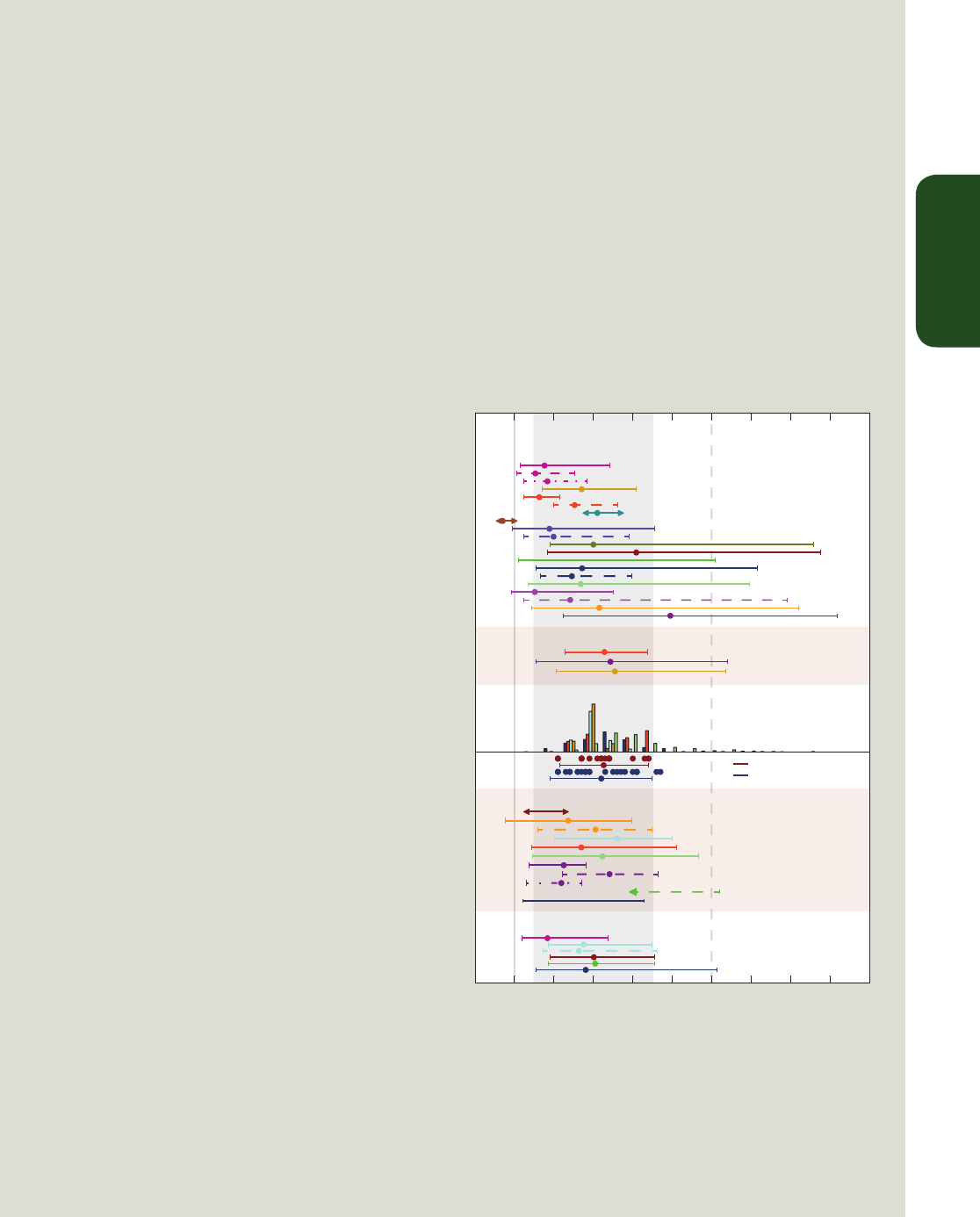
TS
Technical Summary
83
Newer studies of constraints on ECS are based on the observed warming since pre-industrial, analysed using simple
and intermediate complexity models, improved statistical methods and several different and newer data sets.
Together with paleoclimate constraints but without considering the CMIP based evidence these studies show ECS
is likely between 1.5°C to 4.5°C (medium confidence) and extremely unlikely less than 1.0°C. {5.3.1, 5.3.3, 10.8.2;
Boxes 5.2, 12.2}
Estimates based on Atmosphere–Ocean General Circulation Models (AOGCMs) and feedback analysis indicate a
range of 2°C to 4.5°C, with the Coupled Model Intercomparison Project Phase 5 (CMIP5) model mean at 3.2°C,
similar to CMIP3. High climate sensitivities are found in some perturbed parameter ensembles models, but recent
comparisons of perturbed-physics ensembles against the observed climate find that models with ECS values in the
range 3°C to 4°C show the smallest errors for many fields. Relationships between climatological quantities and cli-
mate sensitivity are often found within a specific perturbed parameter ensemble model but in many cases the rela-
tionship is not robust across perturbed parameter ensembles models from different models or in CMIP3 and CMIP5.
The assessed literature suggests that the range of climate sensitivities and transient responses covered by CMIP3
and CMIP5 cannot be narrowed significantly by constraining the models with observations of the mean climate
and variability. Studies based on perturbed parameter
ensembles models and CMIP3 support the conclusion
that a credible representation of the mean climate and
variability is very difficult to achieve with ECSs below
2°C. {9.2.2, 9.7.3; Box 12.2}
New estimates of ECS based on reconstructions and
simulations of the Last Glacial Maximum (21 ka to 19
ka) show that values below 1°C as well as above 6°C are
very unlikely. In some models climate sensitivity differs
between warm and cold climates because of differenc-
es in the representation of cloud feedbacks. Estimates
of an Earth system sensitivity including slow feedbacks
(e.g., ice sheets or vegetation) are even more difficult to
relate to climate sensitivity of the current climate state.
The main limitations of ECS estimates from paleoclimate
states are uncertainties in proxy data, spatial coverage
of the data, uncertainties in some forcings, and struc-
tural limitations in models used in model–data compari-
sons. {5.3, 10.8.2, 12.5.3}
Bayesian methods to constrain ECS or TCR are sensitive
to the assumed prior distributions. They can in principle
yield narrower estimates by combining constraints from
the observed warming trend, volcanic eruptions, model
climatology and paleoclimate, and that has been done
in some studies, but there is no consensus on how this
should be done robustly. This approach is sensitive to
the assumptions regarding the independence of the var-
ious lines of evidence, the possibility of shared biases in
models or feedback estimates and the assumption that
each individual line of evidence is unbiased. The combi-
nation of different estimates in this assessment is based
on expert judgement. {10.8.2; Box 12.2}
Based on the combined evidence from observed climate
change including the observed 20th century warming,
climate models, feedback analysis and paleoclimate, as
discussed above, ECS is likely in the range 1.5°C to 4.5°C
with high confidence. ECS is positive, extremely unlikely
0 1 2 3 4
5
6
7
8
91
0
Equilibrium Climate Sensitivity (°C)
CMIP3AOGCMs
CMIP5AOGCMs
Instrumental
Climatologicalconstraints
Rawmodelrange
Palaeoclimate
Combination
TFE.6 (continued)
TFE.6, Figure 1 | Probability density functions, distributions and ranges for equi-
librium climate sensitivity, based on Figure 10.20b plus climatological constraints
shown in IPCC AR4 (Box AR4 10.2 Figure 1), and results from CMIP5 (Table 9.5).
The grey shaded range marks the likely 1.5°C to 4.5°C range, grey solid line the
extremely unlikely less than 1°C, the grey dashed line the very unlikely greater
than 6°C. See Figure 10.20b and Chapter 10 Supplementary Material for full
caption and details. {Box 12.2, Figure 1}
(continued on next page)
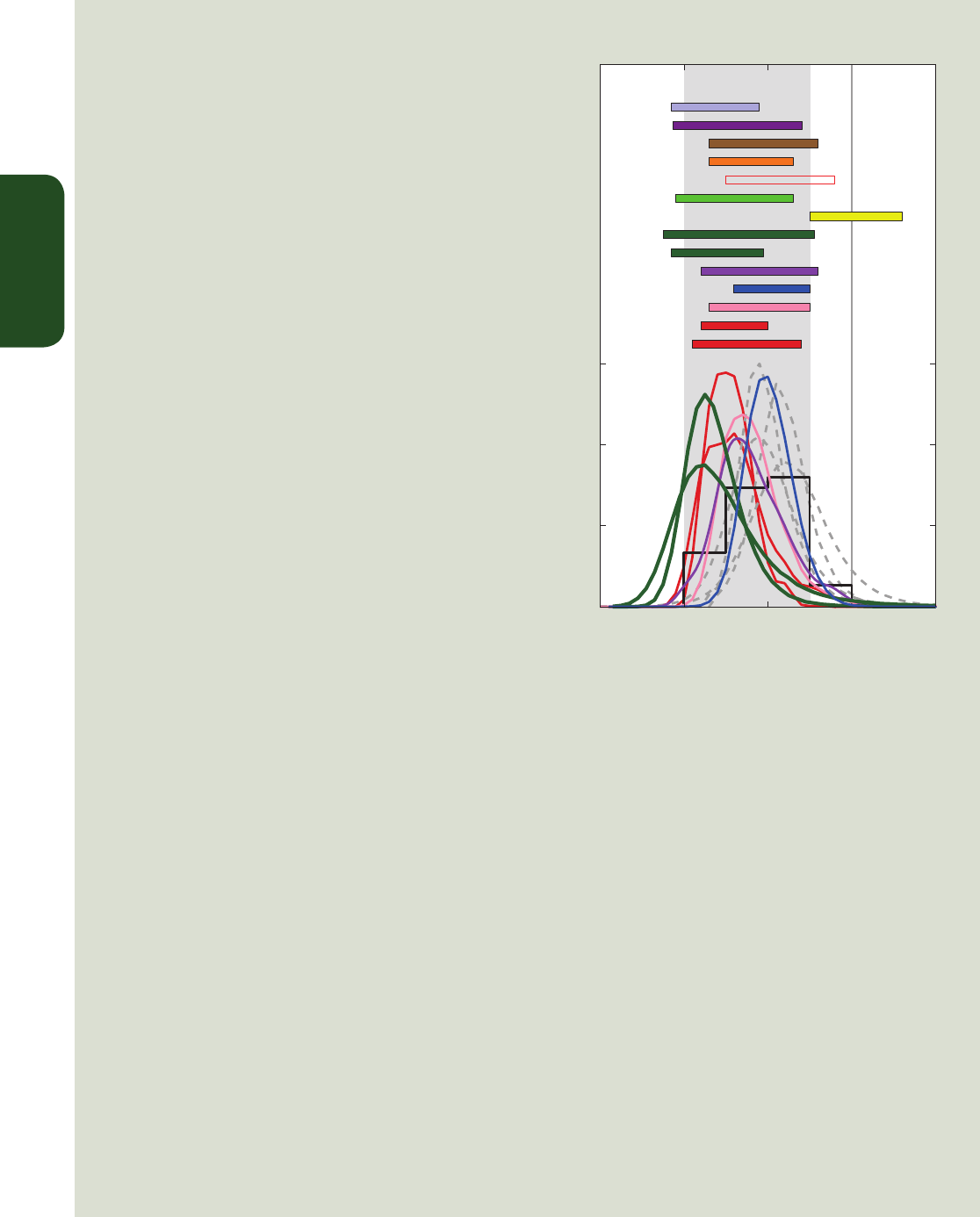
TS
Technical Summary
84
less than 1°C (high confidence), and very unlikely great-
er than 6°C (medium confidence). The tails of the ECS
distribution are now better understood. Multiple lines
of evidence provide high confidence that an ECS value
less than 1°C is extremely unlikely. The upper limit of the
likely range is unchanged compared to AR4. The lower
limit of the likely range of 1.5°C is less than the lower
limit of 2°C in AR4. This change reflects the evidence
from new studies of observed temperature change,
using the extended records in atmosphere and ocean.
These studies suggest a best fit to the observed surface
and ocean warming for ECS values in the lower part of
the likely range. Note that these studies are not purely
observational, because they require an estimate of the
response to RF from models. In addition, the uncertainty
in ocean heat uptake remains substantial. Accounting
for short-term variability in simple models remains chal-
lenging, and it is important not to give undue weight to
any short time period which might be strongly affect-
ed by internal variability. On the other hand, AOGCMs
with observed climatology with ECS values in the upper
part of the 1.5 to 4.5°C range show very good agree-
ment with observed climatology, but the simulation of
key feedbacks like clouds remains challenging in those
models. The estimates from the observed warming,
paleoclimate, and from climate models are consistent
within their uncertainties, each is supported by many
studies and multiple data sets, and in combination they
provide high confidence for the assessed likely range.
Even though this assessed range is similar to previous
reports, confidence today is much higher as a result
of high quality and longer observational records with
a clearer anthropogenic signal, better process under-
standing, more and better understood evidence from
paleoclimate reconstructions, and better climate models
with higher resolution that capture many more processes more realistically. All these lines of evidence individually
support the assessed likely range of 1.5°C to 4.5°C. {3.2, 9.7.3, 10.8; Boxes 9.2, 13.1}
On time scales of many centuries and longer, additional feedbacks with their own intrinsic time scales (e.g., vegeta-
tion, ice sheets) may become important but are not usually modelled in AOGCMs. The resulting equilibrium tem-
perature response to a doubling of CO
2
on millennial time scales or Earth system sensitivity is less well constrained
but likely to be larger than ECS, implying that lower atmospheric CO
2
concentrations are compatible with limiting
warming to below a given temperature level. These slow feedbacks are less likely to be proportional to global mean
temperature change, implying that Earth system sensitivity changes over time. Estimates of Earth system sensitivity
are also difficult to relate to climate sensitivity of the current climate state. {5.3.3, 10.8.2, 12.5.3}
For scenarios of increasing RF, TCR is a more informative indicator of future climate change than ECS. This assess-
ment concludes with high confidence that the TCR is likely in the range 1°C to 2.5°C, close to the estimated 5 to
95% range of CMIP5 (1.2°C to 2.4°C), is positive and extremely unlikely greater than 3°C. As with the ECS, this is
an expert-assessed range, supported by several different and partly independent lines of evidence, each based on
multiple studies, models and data sets. TCR is estimated from the observed global changes in surface temperature,
ocean heat uptake and RF including detection/attribution studies identifying the response patterns to increasing
GHG concentrations, and the results of CMIP3 and CMIP5. Estimating TCR suffers from fewer difficulties in terms of
state- or time-dependent feedbacks, and is less affected by uncertainty as to how much energy is taken up by the
TFE.6, Figure 2 | Probability density functions, distributions and ranges (5 to
95%) for the transient climate response from different studies, based on Figure
10.20a, and results from CMIP5 (black histogram, Table 9.5). The grey shaded
range marks the likely 1°C to 2.5°C range, the grey solid line marks the extremely
unlikely greater than 3°C. See Figure 10.20a and Chapter 10 Supplementary
Material for full caption and details. {Box 12.2, Figure 2}
0123 4
0
0.5
1
1.5
Black histogram
CMIP5 models
Dashed lines
AR4 studies
Transient Climate Response (°C)
Probability / Relative Frequency (°C
−1
)
TFE.6 (continued)
(continued on next page)

TS
Technical Summary
85
ocean. Unlike ECS, the ranges of TCR estimated from the observed warming and from AOGCMs agree well, increas-
ing our confidence in the assessment of uncertainties in projections over the 21st century.
The assessed ranges of ECS and TCR are largely consistent with the observed warming, the estimated forcing and
the projected future warming. In contrast to AR4, no best estimate for ECS is given because of a lack of agreement
on the best estimate across lines of evidence and studies and an improved understanding of the uncertainties in
estimates based on the observed warming. Climate models with ECS values in the upper part of the likely range
show very good agreement with observed climatology, whereas estimates derived from observed climate change
tend to best fit the observed surface and ocean warming for ECS values in the lower part of the likely range. In esti-
mates based on the observed warming the most likely value is sensitive to observational and model uncertainties,
internal climate variability and to assumptions about the prior distribution of ECS. In addition, “best estimate” and
“most likely value” are defined in various ways in different studies. {9.7.1, 10.8.1, 12.5.3; Table 9.5}
TFE.6 (continued)
12
Seasonal-to-interannual predictions typically include the impact of external forcing.
TS.5.4 Near-term Climate Change
Near-term decadal climate prediction provides information not avail-
able from existing seasonal to interannual (months to a year or two)
predictions or from long-term (mid 21st century and beyond) climate
change projections. Prediction efforts on seasonal to interannual time
scales require accurate estimates of the initial climate state with less
focus extended to changes in external forcing
12
, whereas long-term
climate projections rely more heavily on estimations of external forcing
with little reliance on the initial state of internal variability. Estimates
of near-term climate depend on the committed warming (caused by
the inertia of the oceans as they respond to historical external forcing)
the time evolution of internally generated climate variability, and the
future path of external forcing. Near-term predictions out to about a
decade (Figure TS.13) depend more heavily on an accurate depiction of
the internally generated climate variability. {11.1, 12, 14}
Further near-term warming from past emissions is unavoidable owing
to thermal inertia of the oceans. This warming will be increased by
ongoing emissions of GHGs over the near term, and the climate
observed in the near term will also be strongly influenced by the inter-
nally generated variability of the climate system. Previous IPCC Assess-
ments only described climate-change projections wherein the exter-
nally forced component of future climate was included but no attempt
was made to initialize the internally generated climate variability.
Decadal climate predictions, on the other hand, are intended to pre-
dict both the externally forced component of future climate change,
and the internally generated component. Near-term predictions do not
provide detailed information of the evolution of weather. Instead they
can provide estimated changes in the time evolution of the statistics of
near-term climate. {11.1, 11.2.2; Box 11.1; FAQ 11.1}
Retrospective prediction experiments have been used to assess fore-
cast quality. There is high confidence that the retrospective prediction
experiments for forecast periods of up to 10 years exhibit positive skill
when verified against observations over large regions of the planet
and of the global mean. Observation-based initialization of the fore-
casts contributes to the skill of predictions of annual mean tempera-
ture for the first couple of years and to the skill of predictions of the
GMST and the temperature over the North Atlantic, regions of the
South Pacific and the tropical Indian Ocean up to 10 years (high confi-
dence) partly due to a correction of the forced response. Probabilistic
temperature predictions are statistically reliable (see Section 11.2.3 for
definition of reliability) owing to the correct representation of global
trends, but still unreliable at the regional scale when probabilities are
computed from the multi-model ensemble. Predictions initialized over
2000–2005 improve estimates of the recent global mean temperature
hiatus. Predictions of precipitation over continental areas with large
forced trends also exhibit positive skill. {11.2.2, 11.2.3; Box 9.2}
TS.5.4.1 Projected Near-term Changes in Climate
Projections of near-term climate show small sensitivity to GHG sce-
narios compared to model spread, but substantial sensitivity to uncer-
tainties in aerosol emissions, especially on regional scales and for
hydrological cycle variables. In some regions, the local and regional
responses in precipitation and in mean and extreme temperature to
land use change will be larger than those due to large-scale GHGs and
aerosol forcing. These scenarios presume that there are no major vol-
canic eruptions and that anthropogenic aerosol emissions are rapidly
reduced during the near term. {11.3.1, 11.3.2, 11.3.6}
TS.5.4.2 Projected Near-term Changes in Temperature
In the absence of major volcanic eruptions—which would cause sig-
nificant but temporary cooling—and, assuming no significant future
long-term changes in solar irradiance, it is likely that the GMST
anomaly for the period 2016–2035, relative to the reference period of
1986–2005 will be in the range 0.3°C to 0.7°C (medium confidence).
This is based on multiple lines of evidence. This range is consistent

TS
Technical Summary
86
Global mean surface temperature change Atlantic multidecadal variability
CMIP5 Init CMIP5 NoInit
1960 1970 1980 1990 2000 2010
(ºC)
-0.4 0.4
1960 1970 1980 1990 2000 2010
-0.2 0.20.0
Forecast
Year Year
time (yr)
1-4 2-5 3-8 4-7 5-8 6-9 1-4 2-5 3-8 4-7 5-8 6-9
1-4 2-5 3-8 4-7 5-8 6-9 1-4 2-5 3-8 4-7 5-8 6-9
Correlation
0.60.9
rmse (ºC)
Forecast time (yr)
0.00 0.150.100.05
Forecast time (yr)
0.00.3 0.60.9
Forecast time (yr)
0.00 0.150.100.05
0.0
Figure TS.13 | Decadal prediction forecast quality of several climate indices. (Top row)
Time series of the 2- to 5-year average ensemble mean initialized hindcast anoma-
lies and the corresponding non-initialized experiments for three climate indices: global
mean surface temperature (GMST, left) and the Atlantic Multi-decadal Variability (AMV,
right). The observational time series, Goddard Institute of Space Studies Goddard Insti-
tute for Space Studies Surface Temperature Analysis (GISTEMP) global mean tempera-
ture and Extended Reconstructed Sea Surface Tempearture (ERSST) for the AMV, are
represented with dark grey (positive anomalies) and light grey (negative anomalies)
vertical bars, where a 4-year running mean has been applied for consistency with the
time averaging of the predictions. Predicted time series are shown for the CMIP5 Init
(solid) and NoInit (dotted) simulations with hindcasts started every 5 years over the
period 1960–2005. The lower and upper quartile of the multi-model ensemble are plot-
ted using thin lines. The AMV index was computed as the sea surface temperature (SST)
anomalies averaged over the region Equator to 60ºN and 80ºW to 0ºW minus the SST
anomalies averaged over 60ºS to 60ºN. Note that the vertical axes are different for each
time series. (Middle row) Correlation of the ensemble mean prediction with the observa-
tional reference along the forecast time for 4-year averages of the three sets of CMIP5
hindcasts for Init (solid) and NoInit (dashed). The one-sided 95% confidence level with
a t distribution is represented in grey. The effective sample size has been computed
taking into account the autocorrelation of the observational time series. A two-sided
t test (where the effective sample size has been computed taking into account the
autocorrelation of the observational time series) has been used to test the differences
between the correlation of the initialized and non-initialized experiments, but no differ-
ences were found statistically significant with a confidence equal or higher than 90%.
(Bottom row) Root mean square error (RMSE) of the ensemble mean prediction along
the forecast time for 4-year averages of the CMIP5 hindcasts for Init (solid) and NoInit
(dashed). A two-sided F test (where the effective sample size has been computed taking
into account the autocorrelation of the observational time series) has been used to test
the ratio between the RMSE of the Init and NoInit, and those forecast times with differ-
ences statistically significant with a confidence equal or higher than 90% are indicated
with an open square. {Figure 11.3}
with the range obtained by using CMIP5 5 to 95% model trends for
2012–2035. It is also consistent with the CMIP5 5 to 95% range for
all four RCP scenarios of 0.36°C to 0.79°C, using the 2006–2012 refer-
ence period, after the upper and lower bounds are reduced by 10% to
take into account the evidence that some models may be too sensitive
to anthropogenic forcing (see Table TS.1 and Figure TS.14). {11.3.6}
Higher concentrations of GHGs and lower amounts of sulphate aero-
sol lead to greater warming. In the near-term, differences in global
mean surface air temperature across RCP scenarios for a single climate
model are typically smaller than across climate models for a single
RCP scenario. In 2030, the CMIP5 ensemble median values for global
mean temperature differ by at most 0.2°C between the RCP scenarios,
whereas the model spread (defined as the 17 to 83% range ) for each
RCP is around 0.4°C. The inter-scenario spread increases in time and
by 2050 is comparable to the model spread. Regionally, the largest dif-
ferences in surface air temperature between RCP scenarios are found
in the Arctic. {11.3.2. 11.3.6}
The projected warming of global mean temperatures implies high
confidence that new levels of warming relative to 1850-1900 mean
climate will be crossed, particularly under higher GHG emissions sce-
narios. Relative to a reference period of 1850–1900, under RCP4.5 or
RCP6.0, it is more likely than not that the mean GMST for the period
2016–2035 will be more than 1°C above the mean for 1850–1900,
and very unlikely that it will be more than 1.5°C above the 1850–1900
mean (medium confidence). {11.3.6}
A future volcanic eruption similar in size to the 1991 eruption of Mt
Pinatubo would cause a rapid drop in global mean surface air tem-
perature of about 0.5°C in the following year, with recovery over the
next few years. Larger eruptions, or several eruptions occurring close
together in time, would lead to larger and more persistent effects.
{11.3.6}
Possible future changes in solar irradiance could influence the rate at
which GMST increases, but there is high confidence that this influence
will be small in comparison to the influence of increasing concentra-
tions of GHGs in the atmosphere. {11.3.6}
The spatial patterns of near-term warming projected by the CMIP5
models following the RCP scenarios (Figure TS.15) are broadly con-
sistent with the AR4. It is very likely that anthropogenic warming of
surface air temperature over the next few decades will proceed more
rapidly over land areas than over oceans, and it is very likely that
the anthropogenic warming over the Arctic in winter will be greater
than the global mean warming, consistent with the AR4. Relative to
background levels of internally generated variability there is high
confidence that the anthropogenic warming relative to the reference
period is expected to be larger in the tropics and subtropics than in
mid-latitudes. {11.3.2}
It is likely that in the next decades the frequency of warm days and
warm nights will increase in most land regions, while the frequency of
cold days and cold nights will decrease. Models also project increases
in the duration, intensity and spatial extent of heat waves and warm
spells for the near term. These changes may proceed at a different
rate than the mean warming. For example, several studies project that
European high-percentile summer temperatures are projected to warm
faster than mean temperatures (see also TFE.9). {11.3.2}
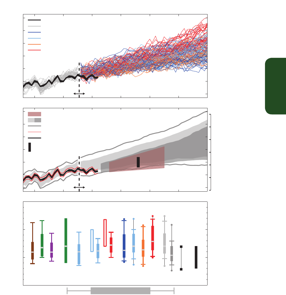
TS
Technical Summary
87
Temperature anomaly (°C)
Global mean temperature near−term projections relative to 1986−2005
RCPsHistorical
(a)
1990 2000 2010 2020 2030 2040 2050
−0.5
0
0.5
1
1.5
2
2.5
Observations (4 datasets)
Historical (42 models)
RCP 2.6 (32 models)
RCP 4.5 (42 models)
RCP 6.0 (25 models)
RCP 8.5 (39 models)
0
1
2
3
Relative to 1850−1900
RCPsHistorical
(b)
Temperature anomaly (°C)
ALL RCPs Assessed likely range
for 2016−2035 mean
Assuming no future
large volcanic eruptions
1990 2000 2010 2020 2030 2040 2050
−0.5
0
0.5
1
1.5
2
2.5
Indicative likely range for annual means
ALL RCPs (5−95% range, two reference periods)
ALL RCPs min−max (299 ensemble members)
Observational uncertainty (HadCRUT4)
Observations (4 datasets)
B1 A1B A2
SRES CMIP3
2.6 4.5 6.0 8.5 ALL
RCPs CMIP5
Key:
%59%5
17−83%
Obs. Constrained
4.5 4.5 8.5A1B
Using trends
Assessed
ALL
(c)
Temperature anomaly (°C)
Projections of 2016−2035 mean
0
0.5
1
1.5
Figure TS.14 | Synthesis of near-term projections of global mean surface air temperature (GMST). (a) Projections of annual mean GMST 1986–2050 (anomalies relative to
1986–2005) under all RCPs from CMIP5 models (grey and coloured lines, one ensemble member per model), with four observational estimates (Hadley Centre/Climatic Research
Unit gridded surface temperature data set 4 (HadCRUT4), European Centre for Medium Range Weather Forecasts (ECMWF) interim re-analysis of the global atmosphere and surface
conditions (ERA-Interim), Goddard Institute for Space Studies Surface Temperature Analysis (GISTEMP), National Oceanic and Atmospheric Administration (NOAA)) for the period
1986–2012 (black lines). (b) As (a) but showing the 5 to 95% range of annual mean CMIP5 projections (using one ensemble member per model) for all RCPs using a reference
period of 1986–2005 (light grey shade) and all RCPs using a reference period of 2006–2012, together with the observed anomaly for (2006–2012) minus (1986–2005) of 0.16°C
(dark grey shade). The percentiles for 2006 onwards have been smoothed with a 5-year running mean for clarity. The maximum and minimum values from CMIP5 using all ensemble
members and the 1986–2005 reference period are shown by the grey lines (also smoothed). Black lines show annual mean observational estimates. The red shaded region shows
the indicative likely range for annual mean GMST during the period 2016–2035 based on the ‘ALL RCPs Assessed’ likely range for the 20-year mean GMST anomaly for 2016–2035,
which is shown as a black bar in both (b) and (c) (see text for details). The temperature scale relative to 1850-1900 mean climate on the right-hand side assumes a warming of
GMST prior to 1986–2005 of 0.61°C estimated from HadCRUT4. (c) A synthesis of projections for the mean GMST anomaly for 2016–2035 relative to 1986–2005. The box and
whiskers represent the 66% and 90% ranges. Shown are: unconstrained SRES CMIP3 and RCP CMIP5 projections; observationally constrained projections for the SRES A1B and,
the RCP4.5 and 8.5 scenarios; unconstrained projections for all four RCP scenarios using two reference periods as in (b) (light grey and dark grey shades), consistent with (b); 90%
range estimated using CMIP5 trends for the period 2012–2035 and the observed GMST anomaly for 2012; an overall likely (>66%) assessed range for all RCP scenarios. The dots
for the CMIP5 estimates show the maximum and minimum values using all ensemble members. The medians (or maximum likelihood estimate; green filled bar) are indicated by a
grey band. (Adapted from Figure 11.25.) See Section 11.3.6 for details. {Figure 11.25}

TS
Technical Summary
88
TS.5.4.3 Projected Near-term Changes in the Water Cycle
Zonal mean precipitation will very likely increase in high and some of
the mid latitudes, and will more likely than not decrease in the subtrop-
ics. At more regional scales precipitation changes may be dominated
by a combination of natural internal variability, volcanic forcing and
anthropogenic aerosol effects. {11.3.2}
Over the next few decades increases in near-surface specific humidity
are very likely. It is likely that there will be increases in evaporation
in many regions. There is low confidence in projected changes in soil
moisture and surface runoff. {11.3.2}
In the near term, it is likely that the frequency and intensity of heavy
precipitation events will increase over land. These changes are primar-
ily driven by increases in atmospheric water vapour content, but also
affected by changes in atmospheric circulation. The impact of anthro-
pogenic forcing at regional scales is less obvious, as regional-scale
changes are strongly affected by natural variability and also depend on
the course of future aerosol emissions, volcanic forcing and land use
changes (see also TFE.9). {11.3.2}
TS.5.4.4 Projected Near-term Changes in Atmospheric Circulation
Internally generated climate variability and multiple RF agents (e.g.,
volcanoes, GHGs, ozone and anthropogenic aerosols) will all contrib-
ute to near-term changes in the atmospheric circulation. For example,
it is likely that the annual mean Hadley Circulation and the SH mid-lat-
itude westerlies will shift poleward, while it is likely that the projected
recovery of stratospheric ozone and increases in GHG concentrations
will have counteracting impacts on the width of the Hadley Circula-
tion and the meridional position of the SH storm track. Therefore it is
unlikely that they will continue to expand poleward as rapidly as in
recent decades. {11.3.2}
There is low confidence in near-term projections of the position and
strength of NH storm tracks. Natural variations are larger than the pro-
jected impact of GHGs in the near term. {11.3.2}
There is low confidence in basin-scale projections of changes in inten-
sity and frequency of tropical cyclones in all basins to the mid-21st
century. This low confidence reflects the small number of studies
exploring near-term tropical cyclone activity, the differences across
published projections of tropical cyclone activity, and the large role for
natural variability. There is low confidence in near-term projections for
increased tropical cyclone intensity in the Atlantic; this projection is in
part due to projected reductions in aerosol loading. {11.3.2}
TS.5.4.5 Projected Near-term Changes in the Ocean
It is very likely that globally averaged surface and vertically averaged
ocean temperatures will increase in the near-term. In the absence of
multiple major volcanic eruptions, it is very likely that globally aver-
aged surface and depth-averaged temperatures averaged for 2016–
2035 will be warmer than those averaged over 1986–2005. {11.3.3}
It is likely that salinity will increase in the tropical and (especially) sub-
tropical Atlantic, and decrease in the western tropical Pacific over the
next few decades. Overall, it is likely that there will be some decline
in the Atlantic Meridional Overturning Circulation by 2050 (medium
confidence). However, the rate and magnitude of weakening is very
uncertain and decades when this circulation increases are also to be
expected. {11.3.3}
TS.5.4.6 Projected Near-term Changes in the Cryosphere
A nearly ice-free Arctic Ocean (sea ice extent less than 10
6
km
2
for at
least five consecutive years) in September is likely before mid-century
under RCP8.5 (medium confidence). This assessment is based on a
subset of models that most closely reproduce the climatological mean
state and 1979 to 2012 trend of Arctic sea ice cover. It is very likely that
there will be further shrinking and thinning of Arctic sea ice cover, and
decreases of northern high-latitude spring time snow cover and near
surface permafrost as GMST rises (Figures TS.17 and TS.18). There is
low confidence in projected near-term decreases in the Antarctic sea
ice extent and volume. {11.3.4}
TS.5.4.7 Possibility of Near-term Abrupt Changes in Climate
There are various mechanisms that could lead to changes in global or
regional climate that are abrupt by comparison with rates experienced
in recent decades. The likelihood of such changes is generally lower
for the near term than for the long term. For this reason the relevant
mechanisms are primarily assessed in the TS.5 sections on long-term
changes and in TFE.5. {11.3.4}
TS.5.4.8 Projected Near-term Changes in Air Quality
The range in projections of air quality (O
3
and PM
2.5
in surface air) is
driven primarily by emissions (including CH
4
), rather than by physi-
cal climate change (medium confidence). The response of air qual-
ity to climate-driven changes is more uncertain than the response
to emission-driven changes (high confidence). Globally, warming
decreases background surface O
3
(high confidence). High CH
4
levels
(such as RCP8.5 and SRES A2) can offset this decrease, raising 2100
background surface O
3
on average by about 8 ppb (25% of current
levels) relative to scenarios with small CH
4
changes (such as RCP4.5
and RCP6.0) (high confidence). On a continental scale, projected air
pollution levels are lower under the new RCP scenarios than under the
SRES scenarios because the SRES did not incorporate air quality legis-
lation (high confidence). {11.3.5, 11.3.5.2; Figures 11.22 and 11.23ab,
AII.4.2, AII.7.1–AII.7.4}
Observational and modelling evidence indicates that, all else being
equal, locally higher surface temperatures in polluted regions will
trigger regional feedbacks in chemistry and local emissions that will
increase peak levels of O
3
and PM
2.5
(medium confidence). Local emis-
sions combined with background levels and with meteorological con-
ditions conducive to the formation and accumulation of pollution are
known to produce extreme pollution episodes on local and regional
scales. There is low confidence in projecting changes in meteorologi-
cal blocking associated with these extreme episodes. For PM
2.5
, cli-
mate change may alter natural aerosol sources (wildfires, wind-lofted
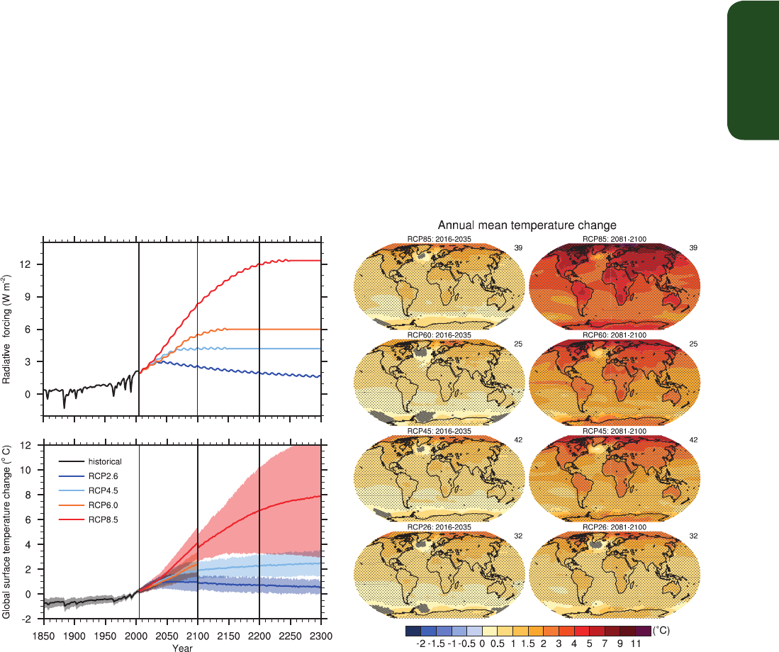
TS
Technical Summary
89
dust, biogenic precursors) as well as precipitation scavenging, but no
confidence level is attached to the overall impact of climate change on
PM
2.5
distributions. {11.3.5, 11.3.5.2; Box 14.2}
TS.5.5 Long-term Climate Change
TS.5.5.1 Projected Long-term Changes in Global Temperature
Global mean temperatures will continue to rise over the 21st century
under all of the RCPs. From around the mid-21st century, the rate of
global warming begins to be more strongly dependent on the scenario
(Figure TS.15). {12.4.1}
Under the assumptions of the concentration-driven RCPs, GMSTs for
2081–2100, relative to 1986–2005 will likely be in the 5 to 95% range
of the CMIP5 models; 0.3°C to 1.7°C (RCP2.6), 1.1 to 2.6°C (RCP4.5),
1.4°C to 3.1°C (RCP6.0), 2.6°C to 4.8°C (RCP8.5) (see Table TS.1). With
high confidence, the 5 to 95% range of CMIP5 is assessed as likely
rather than very likely based on the assessment of TCR (see TFE.6).
42 models
39
25
42
32
12
17
12
Figure TS.15 | (Top left) Total global mean radiative forcing for the four RCP scenarios based on the Model for the Assessment of Greenhouse-gas Induced Climate Change
(MAGICC) energy balance model. Note that the actual forcing simulated by the CMIP5 models differs slightly between models. (Bottom left) Time series of global annual mean
surface air temperature anomalies (relative to 1986–2005) from CMIP5 concentration-driven experiments. Projections are shown for each RCP for the multi-model mean (solid
lines) and ±1.64 standard deviation (5 to 95%) across the distribution of individual models (shading), based on annual means. The 1.64 standard deviation range based on the 20
yr averages 2081–2100, relative to 1986–2005, are interpreted as likely changes for the end of the 21st century. Discontinuities at 2100 are due to different numbers of models
performing the extension runs beyond the 21st century and have no physical meaning. Numbers in the same colours as the lines indicate the number of different models contribut-
ing to the different time periods. Maps: Multi-model ensemble average of annual mean surface air temperature change (compared to 1986–2005 base period) for 2016–2035
and 2081–2100, for RCP2.6, 4.5, 6.0 and 8.5. Hatching indicates regions where the multi-model mean signal is less than one standard deviation of internal variability. Stippling
indicates regions where the multi-model mean signal is greater than two standard deviations of internal variability and where 90% of the models agree on the sign of change. The
number of CMIP5 models used is indicated in the upper right corner of each panel. Further detail regarding the related Figures SPM.7a and SPM.8.a is given in the TS Supplementary
Material. {Box 12.1; Figures 12.4, 12.5, 12.11; Annex I}
The 5 to 95% range of CMIP5 for global mean temperature change
is also assessed as likely for mid-21st century, but only with medium
confidence. With respect to 1850–1900 mean conditions, global
temperatures averaged in the period 2081–2100 are projected to likely
exceed 1.5°C above 1850–1900 values for RCP4.5, RCP6.0 and RCP8.5
(high confidence) and are likely to exceed 2°C above 1850–1900
values for RCP6.0 and RCP8.5 (high confidence). Temperature change
above 2°C relative to 1850–1900 under RCP2.6 is unlikely (medium
confidence). Warming above 4°C by 2081–2100 is unlikely in all RCPs
(high confidence) except for RCP8.5, where it is about as likely as not
(medium confidence). {12.4.1; Tables 12.2, 12.3}
TS.5.5.2 Projected Long-term Changes in Regional Temperature
There is very high confidence that globally averaged changes over land
will exceed changes over the ocean at the end of the 21st century by
a factor that is likely in the range 1.4 to 1.7. In the absence of a strong
reduction in the Atlantic Meridional Overturning, the Arctic region
is projected to warm most (very high confidence) (Figure TS.15). As

TS
Technical Summary
90
GMST rises, the pattern of atmospheric zonal mean temperatures show
warming throughout the troposphere and cooling in the stratosphere,
consistent with previous assessments. The consistency is especially
clear in the tropical upper troposphere and the northern high latitudes.
{12.4.3; Box 5.1}
It is virtually certain that, in most places, there will be more hot
and fewer cold temperature extremes as global mean temperatures
increase. These changes are expected for events defined as extremes
on both daily and seasonal time scales. Increases in the frequency,
duration and magnitude of hot extremes along with heat stress are
expected; however, occasional cold winter extremes will continue to
occur. Twenty-year return values of low-temperature events are pro-
jected to increase at a rate greater than winter mean temperatures
in most regions, with the largest changes in the return values of low
temperatures at high latitudes. Twenty-year return values for high-
temperature events are projected to increase at a rate similar to or
greater than the rate of increase of summer mean temperatures in
most regions. Under RCP8.5 it is likely that, in most land regions, a cur-
rent 20-year high-temperature event will occur more frequently by the
end of the 21st century (at least doubling its frequency, but in many
regions becoming an annual or 2-year event) and a current 20-year
low-temperature event will become exceedingly rare (See also TFE.9).
{12.4.3}
Models simulate a decrease in cloud amount in the future over most of
the tropics and mid-latitudes, due mostly to reductions in low clouds.
Changes in marine boundary layer clouds are most uncertain. Increases
in cloud fraction and cloud optical depth and therefore cloud reflection
are simulated in high latitudes, poleward of 50°. {12.4.3}
TS.5.5.3 Projected Long-term Changes in Atmospheric Circulation
Mean sea level pressure is projected to decrease in high latitudes and
increase in the mid-latitudes as global temperatures rise. In the trop-
ics, the Hadley and Walker Circulations are likely to slow down. Pole-
ward shifts in the mid-latitude jets of about 1 to 2 degrees latitude
are likely at the end of the 21st century under RCP8.5 in both hemi-
spheres (medium confidence), with weaker shifts in the NH. In austral
summer, the additional influence of stratospheric ozone recovery in
the SH opposes changes due to GHGs there, though the net response
varies strongly across models and scenarios. Substantial uncertainty
and thus low confidence remains in projecting changes in NH storm
tracks, especially for the North Atlantic basin. The Hadley Cell is likely
to widen, which translates to broader tropical regions and a pole-
ward encroachment of subtropical dry zones. In the stratosphere, the
Brewer–Dobson circulation is likely to strengthen. {12.4.4}
2046–2065 2081–2100
Scenario Mean Likely range
c
Mean Likely range
c
Global Mean Surface
Temperature Change (°C)
a
RCP2.6 1.0 0.4 to 1.6 1.0 0.3 to 1.7
RCP4.5 1.4 0.9 to 2.0 1.8 1.1 to 2.6
RCP6.0 1.3 0.8 to 1.8 2.2 1.4 to 3.1
RCP8.5 2.0 1.4 to 2.6 3.7 2.6 to 4.8
Scenario Mean Likely range
d
Mean Likely range
d
Global Mean Sea Level
Rise (m)
b
RCP2.6 0.24 0.17 to 0.32 0.40 0.26 to 0.55
RCP4.5 0.26 0.19 to 0.33 0.47 0.32 to 0.63
RCP6.0 0.25 0.18 to 0.32 0.48 0.33 to 0.63
RCP8.5 0.30 0.22 to 0.38 0.63 0.45 to 0.82
Notes:
a
Based on the CMIP5 ensemble; anomalies calculated with respect to 1986–2005. Using HadCRUT4 and its uncertainty estimate (5−95% confidence interval), the observed warming to the
reference period 1986−2005 is 0.61 [0.55 to 0.67] °C from 1850−1900, and 0.11 [0.09 to 0.13] °C from 1980−1999, the reference period for projections used in AR4. Likely ranges have not been
assessed here with respect to earlier reference periods because methods are not generally available in the literature for combining the uncertainties in models and observations. Adding projected
and observed changes does not account for potential effects of model biases compared to observations, and for natural internal variability during the observational reference period. {2.4; 11.2;
Tables 12.2 and 12.3}
b
Based on 21 CMIP5 models; anomalies calculated with respect to 1986–2005. Where CMIP5 results were not available for a particular AOGCM and scenario, they were estimated as explained
in Chapter 13, Table 13.5. The contributions from ice sheet rapid dynamical change and anthropogenic land water storage are treated as having uniform probability distributions, and as largely
independent of scenario. This treatment does not imply that the contributions concerned will not depend on the scenario followed, only that the current state of knowledge does not permit a
quantitative assessment of the dependence. Based on current understanding, only the collapse of marine-based sectors of the Antarctic ice sheet, if initiated, could cause global mean sea level to
rise substantially above the likely range during the 21st century. There is medium confidence that this additional contribution would not exceed several tenths of a metre of sea level rise during
the 21st century.
c
Calculated from projections as 5−95% model ranges. These ranges are then assessed to be likely ranges after accounting for additional uncertainties or different levels of confidence in models.
For projections of global mean surface temperature change in 2046−2065 confidence is medium, because the relative importance of natural internal variability, and uncertainty in non-greenhouse
gas forcing and response, are larger than for 2081−2100. The likely ranges for 2046−2065 do not take into account the possible influence of factors that lead to the assessed range for near-term
(2016−2035) global mean surface temperature change that is lower than the 5−95% model range, because the influence of these factors on longer term projections has not been quantified due
to insufficient scientific understanding. {11.3}
d
Calculated from projections as 5−95% model ranges. These ranges are then assessed to be likely ranges after accounting for additional uncertainties or different levels of confidence in models.
For projections of global mean sea level rise confidence is medium for both time horizons.
Table TS.1 | Projected change in global mean surface air temperature and global mean sea level rise for the mid- and late 21st century relative to the reference period of
1986–2005. {12.4.1; Tables 12.2,13.5}
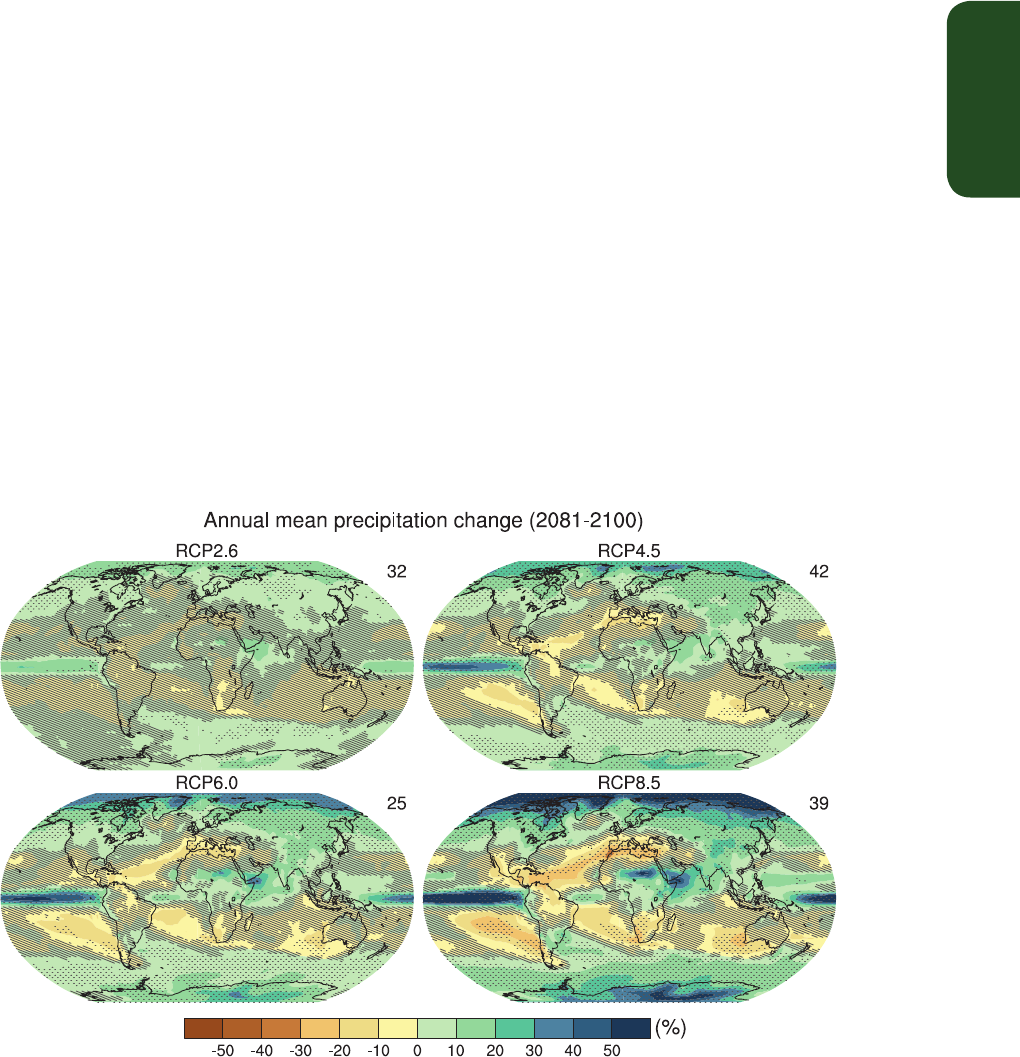
TS
Technical Summary
91
TS.5.5.4 Projected Long-term Changes in the Water Cycle
On the planetary scale, relative humidity is projected to remain roughly
constant, but specific humidity to increase in a warming climate. The
projected differential warming of land and ocean promotes changes in
atmospheric moistening that lead to small decreases in near-surface
relative humidity over most land areas with the notable exception
of parts of tropical Africa (medium confidence) (see TFE.1, Figure 1).
{12.4.5}
It is virtually certain that, in the long term, global precipitation will
increase with increased GMST. Global mean precipitation will increase
at a rate per °C smaller than that of atmospheric water vapour. It will
likely increase by 1 to 3% °C
–1
for scenarios other than RCP2.6. For
RCP2.6 the range of sensitivities in the CMIP5 models is 0.5 to 4% °C
–1
at the end of the 21st century. {7.6.2, 7.6.3, 12.4.1}
Changes in average precipitation in a warmer world will exhibit sub-
stantial spatial variation under RCP8.5. Some regions will experience
increases, other regions will experience decreases and yet others will
not experience significant changes at all (see Figure TS.16). There
is high confidence that the contrast of annual mean precipitation
between dry and wet regions and that the contrast between wet
and dry seasons will increase over most of the globe as temperatures
increase. The general pattern of change indicates that high latitudes
are very likely to experience greater amounts of precipitation due to
the increased specific humidity of the warmer troposphere as well as
increased transport of water vapour from the tropics by the end of this
Figure TS.16 | Maps of multi-model results for the scenarios RCP2.6, RCP4.5, RCP6.0 and RCP8.5 in 2081–2100 of average percent change in mean precipitation. Changes are
shown relative to 1986–2005. The number of CMIP5 models to calculate the multi-model mean is indicated in the upper right corner of each panel. Hatching indicates regions
where the multi- model mean signal is less than 1 standard deviation of internal variability. Stippling indicates regions where the multi- model mean signal is greater than 2
standard deviations of internal variability and where 90% of models agree on the sign of change (see Box 12.1). Further detail regarding the related Figure SPM.8b is given in the
TS Supplementary Material. {Figure 12.22; Annex I}
century under the RCP8.5 scenario. Many mid-latitude and subtropical
arid and semi-arid regions will likely experience less precipitation and
many moist mid-latitude regions will likely experience more precipita-
tion by the end of this century under the RCP8.5 scenario. Maps of
precipitation change for the four RCP scenarios are shown in Figure
TS.16. {12.4.2, 12.4.5}
Globally, for short-duration precipitation events, a shift to more intense
individual storms and fewer weak storms is likely as temperatures
increase. Over most of the mid-latitude land masses and over wet tropi-
cal regions, extreme precipitation events will very likely be more intense
and more frequent in a warmer world. The global average sensitivity
of the 20-year return value of the annual maximum daily precipitation
ranges from 4% °C
–1
of local temperature increase (average of CMIP3
models) to 5.3% °C
–1
of local temperature increase (average of CMIP5
models), but regionally there are wide variations. {12.4.2, 12.4.5}
Annual surface evaporation is projected to increase as global tempera-
tures rise over most of the ocean and is projected to change over land
following a similar pattern as precipitation. Decreases in annual runoff
are likely in parts of southern Europe, the Middle East and southern
Africa by the end of this century under the RCP8.5 scenario. Increases in
annual runoff are likely in the high northern latitudes corresponding to
large increases in winter and spring precipitation by the end of the 21st
century under the RCP8.5 scenario. Regional to global-scale projected
decreases in soil moisture and increased risk of agricultural drought
are likely in presently dry regions and are projected with medium confi-
dence by the end of this century under the RCP8.5 scenario. Prominent
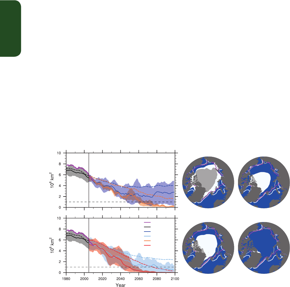
TS
Technical Summary
92
areas of projected decreases in evaporation include southern Africa
and northwestern Africa along the Mediterranean. Soil moisture drying
in the Mediterranean and southern African regions is consistent with
projected changes in Hadley Circulation and increased surface tem-
peratures, so surface drying in these regions as global temperatures
increase is likely with high confidence by the end of this century under
the RCP8.5 scenario. In regions where surface moistening is projected,
changes are generally smaller than natural variability on the 20-year
time scale. A summary of the projected changes in the water cycle from
the CMIP5 models is shown in TFE.1, Figure 1. {12.4.5; Box 12.1}
TS.5.5.5 Projected Long-term Changes in the Cryosphere
It is very likely that the Arctic sea ice cover will continue shrinking and
thinning year-round in the course of the 21st century as GMST rises.
At the same time, in the Antarctic, a decrease in sea ice extent and
volume is expected, but with low confidence. The CMIP5 multi-model
projections give average reductions in Arctic sea ice extent for 2081–
2100 compared to 1986–2005 ranging from 8% for RCP2.6 to 34%
for RCP8.5 in February and from 43% for RCP2.6 to 94% for RCP8.5 in
September (medium confidence) (Figure TS.17). A nearly ice-free Arctic
Ocean (sea ice extent less than 10
6
km
2
for at least five consecutive
years) in September before mid-century is likely under RCP8.5 (medium
confidence), based on an assessment of a subset of models that most
closely reproduce the climatological mean state and 1979–2012 trend
of the Arctic sea ice cover. Some climate projections exhibit 5- to
10-year periods of sharp summer Arctic sea ice decline—even steeper
than observed over the last decade—and it is likely that such instances
of rapid ice loss will occur in the future. There is little evidence in global
climate models of a tipping point (or critical threshold) in the transition
from a perennially ice-covered to a seasonally ice-free Arctic Ocean
beyond which further sea ice loss is unstoppable and irreversible. In
the Antarctic, the CMIP5 multi-model mean projects a decrease in sea
ice extent that ranges from 16% for RCP2.6 to 67% for RCP8.5 in
February and from 8% for RCP2.6 to 30% for RCP8.5 in September
for 2081–2100 compared to 1986–2005. There is, however, low con-
fidence in those projections because of the wide inter-model spread
and the inability of almost all of the available models to reproduce the
overall increase of the Antarctic sea ice areal coverage observed during
the satellite era. {12.4.6, 12.5.5}
It is very likely that NH snow cover will reduce as global temperatures
rise over the coming century. A retreat of permafrost extent with rising
global temperatures is virtually certain. Snow cover changes result
from precipitation and ablation changes, which are sometimes oppo-
site. Projections of the NH spring snow covered area by the end of the
21st century vary between a decrease of 7 [3 to 10] % (RCP2.6) and 25
[18 to 32] % (RCP8.5) (Figure TS.18), but confidence is those numbers
is only medium because snow processes in global climate models are
strongly simplified. The projected changes in permafrost are a response
not only to warming, but also to changes in snow cover, which exerts a
control on the underlying soil. By the end of the 21st century, diagnosed
near-surface permafrost area is projected to decrease by between 37%
(RCP2.6) to 81% (RCP8.5) (medium confidence). {12.4.6}
observations
historical
RCP2.6
RCP4.5
RCP8.5
RCP6.0
NH September sea-ice extent
39(5)
29(3)
37(5)
39(5)
21(2)
39(5)
RCP2.6 RCP6.0
RCP4.5
RCP8.5
()
()
2081–2100
Figure TS.17 | Northern Hemisphere (NH) sea ice extent in September over the late 20th century and the whole 21st century for the scenarios RCP2.6, RCP4.5, RCP6.0 and RCP8.5
in the CMIP5 models, and corresponding maps of multi-model results in 2081–2100 of NH September sea ice extent. In the time series, the number of CMIP5 models to calculate
the multi-model mean is indicated (subset in brackets). Time series are given as 5-year running means. The projected mean sea ice extent of a subset of models that most closely
reproduce the climatological mean state and 1979–2012 trend of the Arctic sea ice is given (solid lines), with the minimum to maximum range of the subset indicated with shading.
Black (grey shading) is the modelled historical evolution using historical reconstructed forcings. The CMIP5 multi-model mean is indicated with dashed lines. In the maps, the CMIP5
multi-model mean is given in white and the results for the subset in grey. Filled areas mark the averages over the 2081–2100 period, lines mark the sea ice extent averaged over
the 1986–2005 period. The observed sea ice extent is given in pink as a time series and averaged over 1986–2005 as a pink line in the map. Further detail regarding the related
Figures SPM.7b and SPM.8c is given in the TS Supplementary Material. {Figures 12.18, 12.29, 12.31}
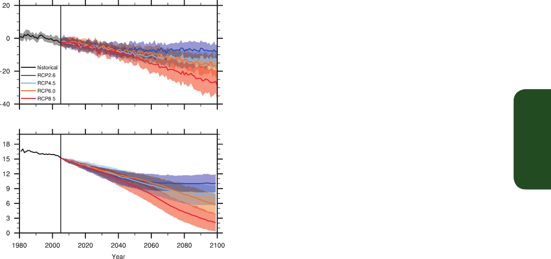
TS
Technical Summary
93
TS.5.5.6 Projected Long-term Changes in the Ocean
Over the course of the 21st century, the global ocean will warm in
all RCP scenarios. The strongest ocean warming is projected for the
surface in subtropical and tropical regions. At greater depth the
warming is projected to be most pronounced in the Southern Ocean.
Best estimates of ocean warming in the top one hundred metres are
about 0.6°C (RCP2.6) to 2.0°C (RCP8.5), and 0.3°C (RCP2.6) to 0.6°C
(RCP8.5) at a depth of about 1 km by the end of the 21st century. For
RCP4.5 by the end of the 21st century, half of the energy taken up by
the ocean is in the uppermost 700 m, and 85% is in the uppermost
2000 m. Due to the long time scales of this heat transfer from the
surface to depth, ocean warming will continue for centuries, even if
GHG emissions are decreased or concentrations kept constant, and will
result in a continued contribution to sea level rise (see Section TS5.7).
{12.4.3, 12.4.7}
TS.5.6 Long-term Projections of Carbon and Other
Biogeochemical Cycles
Projections of the global carbon cycle to 2100 using the CMIP5 ESMs
represent a wider range of complex interactions between the carbon
cycle and the physical climate system. {6}
With very high confidence, ocean carbon uptake of anthropogenic CO
2
will continue under all four RCPs through to 2100, with higher uptake
in higher concentration pathways. The future evolution of the land
carbon uptake is much more uncertain. A majority of CMIP5 ESMs proj-
ect a continued net carbon uptake by land ecosystems through 2100.
Yet, a minority of models simulate a net CO
2
source to the atmosphere
by 2100 due to the combined effect of climate change and land use
change. In view of the large spread of model results and incomplete
process representation, there is low confidence on the magnitude of
modelled future land carbon changes. {6.4.3}
There is high confidence that climate change will partially offset
increases in global land and ocean carbon sinks caused by rising atmos-
pheric CO
2
. Yet, there are regional differences among CMIP5 ESMs in
the response of ocean and land CO
2
fluxes to climate. There is high
agreement between models that tropical ecosystems will store less
carbon in a warmer climate. There is medium agreement between the
CMIP5 ESMs that at high latitudes warming will increase land carbon
storage, although none of these models accounts for decomposition of
carbon in permafrost which may offset increased land carbon storage.
There is high confidence that reductions in permafrost extent due to
warming will cause thawing of some currently frozen carbon. However,
there is low confidence on the magnitude of carbon losses through CO
2
and CH
4
emissions to the atmosphere with a range from 50 to 250 PgC
between 2000 and 2100 for RCP8.5. {6.4.2, 6.4.3}
The loss of carbon from frozen soils constitutes a positive radiative
feedback that is missing in current coupled ESM projections. There is
high agreement between CMIP5 ESMs that ocean warming and cir-
culation changes will reduce the rate of ocean carbon uptake in the
Southern Ocean and North Atlantic, but that carbon uptake will never-
theless persist in those regions. {6.4.2}
It is very likely, based on new experimental results and modelling,
that nutrient shortage will limit the effect of rising atmospheric CO
2
on future land carbon sinks for the four RCP scenarios. There is high
confidence that low nitrogen availability will limit carbon storage on
land even when considering anthropogenic nitrogen deposition. The
role of phosphorus limitation is more uncertain. {6.4.6}
For the ESMs simulations driven by CO
2
concentrations, representation
of the land and ocean carbon cycle allows quantification of the fossil
fuel emissions compatible with the RCP scenarios. Between 2012 and
2100, ESM results imply cumulative compatible fossil fuel emissions of
270 [140 to 410] PgC for RCP2.6, 780 [595 to 1005] PgC for RCP4.5,
1060 [840 to 1250] PgC for RCP6.0 and 1685 [1415 to 1910] PgC for
RCP8.5 (values quoted to nearest 5 PgC, range ±1 standard devia-
tion derived from CMIP5 model results) (Figure TS.19). For RCP2.6, the
models project an average 50% (range 14 to 96%) emission reduction
by 2050 relative to 1990 levels. By the end of the 21st century, about
half of the models infer emissions slightly above zero, while the other
half infer a net removal of CO
2
from the atmosphere (see also Box
TS.7). {6.4.3; Table 6.12}
When forced with RCP8.5 CO
2
emissions, as opposed to the RCP8.5
CO
2
concentrations, CMIP5 ESMs with interactive carbon cycles simu-
late, on average, a 50 (–140 to +210) ppm larger atmospheric CO
2
concentration and a 0.2 (–0.4 to +0.9) °C larger global surface tem-
perature increase by 2100 (CMIP5 model spread ). {12.4.8}
(%)
Snow cover extent change
(10
6
km
2
)
Near surface permafrost area
Figure TS.18 | (Top) Northern Hemisphere (NH) spring (March to April average) rela-
tive snow-covered area (RSCA) in CMIP5, obtained by dividing the simulated 5-year
box smoothed spring snow-covered area (SCA) by the simulated average spring SCA
of 1986–2005 reference period. (Bottom) NH diagnosed near-surface permafrost area
in CMIP5, using 20-year average monthly surface air temperatures and snow depths.
Lines indicate the multi model average, shading indicates the inter-model spread (one
standard deviation). {Figures 12.32, 12.33}
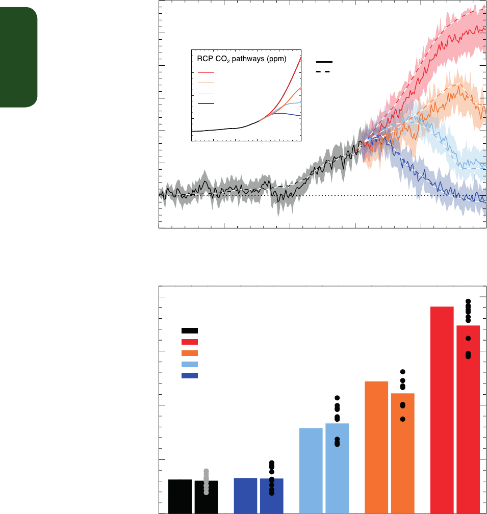
TS
Technical Summary
94
1850 1900 1950 2000 2050 2100
Years
-5
0
5
10
15
20
25
30
(PgC yr
-1
)
Fossil-fuel emissions
RCP8.5
RCP6.0
RCP4.5
RCP2.6
CMIP5 mean
IAM scenario
1850 1900 1950 2000 2050 2100
200
400
600
800
1000
0
500
1000
1500
2000
(PgC)
Cumulative fossil-fuel emissions
Historical
ESMs
IMAGE
ESMs
GCAM
ESMs
AIM
ESMs
MESSAGE
ESMs
Historical emission inventories (1860-2005)
RCP8.5 (2006-2100)
RCP6.0 (2006-2100)
RCP4.5 (2006-2100)
RCP2.6 (2006-2100)
Figure TS.19 | Compatible fossil fuel emissions simulated by the CMIP5 models for the four RCP scenarios. (Top) Time series of annual emission (PgC yr
–1
). Dashed lines represent
the historical estimates and RCP emissions calculated by the Integrated Assessment Models (IAMs) used to define the RCP scenarios, solid lines and plumes show results from CMIP5
Earth System Models (ESMs, model mean, with one standard deviation shaded). (Bottom) Cumulative emissions for the historical period (1860–2005) and 21st century (defined in
CMIP5 as 2006–2100) for historical estimates and RCP scenarios. Left bars are cumulative emissions from the IAMs, right bars are the CMIP5 ESMs multi-model mean estimate
and dots denote individual ESM results. From the CMIP5 ESMs results, total carbon in the land-atmosphere–ocean system can be tracked and changes in this total must equal fossil
fuel emissions to the system. Hence the compatible emissions are given by cumulative emissions = ΔC
A
+ ΔC
L
+ ΔC
O
, while emission rate = d/dt [C
A
+C
L
+ C
O
], where C
A
, C
L
, C
O
are carbon stored in atmosphere, land and ocean respectively. Other sources and sinks of CO
2
such as from volcanism, sedimentation or rock weathering, which are very small on
centennial time scales are not considered here. {Box 6.4; Figure 6.25}
It is virtually certain that the increased storage of carbon by the ocean
will increase acidification in the future, continuing the observed trends
of the past decades. Ocean acidification in the surface ocean will
follow atmospheric CO
2
and it will also increase in the deep ocean as
CO
2
continues to penetrate the abyss. The CMIP5 models consistently
project worldwide increased ocean acidification to 2100 under all
RCPs. The corresponding decrease in surface ocean pH by the end of
21st century is 0.065 (0.06 to 0.07) for RCP2.6, 0.145 (0.14 to 0.15)
for RCP4.5, 0.203 (0.20 to 0.21) for RCP6.0 and 0.31 (0.30 to 0.32)
for RCP8.5 (CMIP5 model spread) (Figure TS.20). Surface waters are
projected to become seasonally corrosive to aragonite in parts of the
Arctic and in some coastal upwelling systems within a decade, and
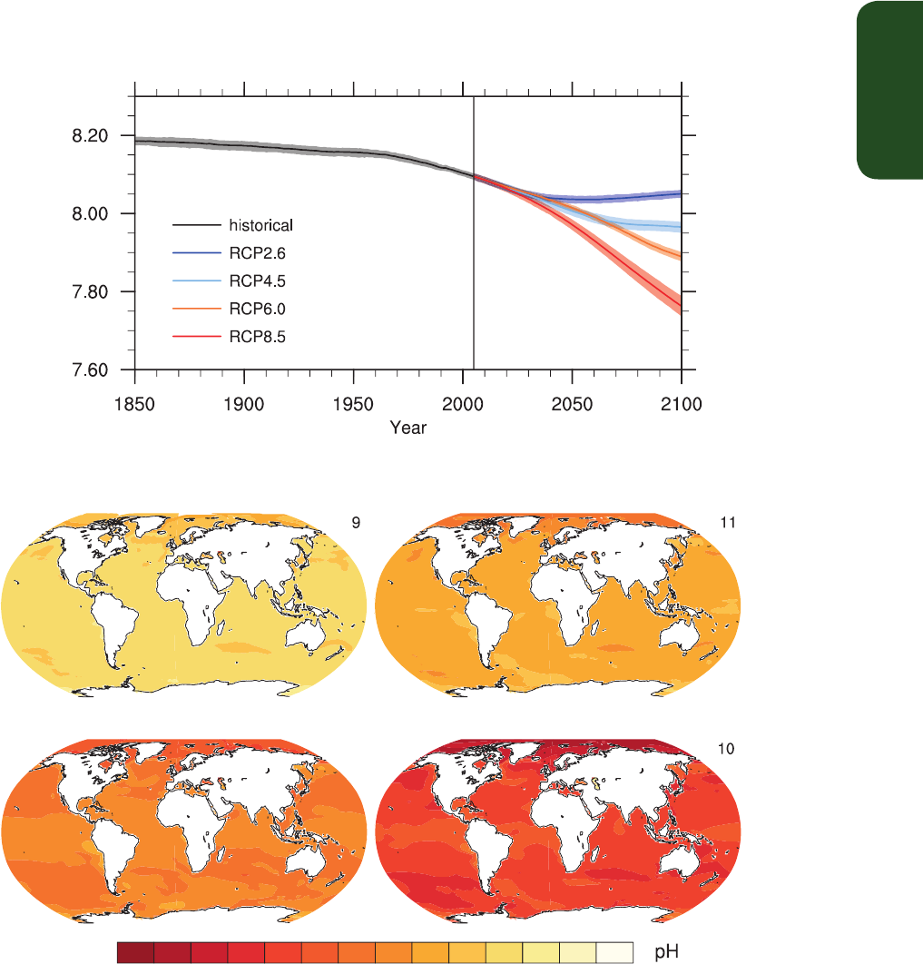
TS
Technical Summary
95
Figure TS.20 | (a) Time series (model averages and minimum to maximum ranges) and (b) maps of multi-model surface ocean pH for the scenarios RCP2.6, RCP4.5, RCP6.0 and
RCP8.5 in 2081–2100. The maps in (b) show change in global ocean surface pH in 2081–2100 relative to 1986–2005. The number of CMIP5 models to calculate the multi-model
mean is indicated in the upper right corner of each panel. Further detail regarding the related Figures SPM.7c and SPM.8.d is given in the TS Supplementary Material. {Figure 6.28}
(a)
(b)
12
9
4
10
11
Change in ocean surface pH (2081-2100)
RCP2.6 RCP4.5
RCP6.0 RCP8.5
4
pH
Global ocean surface pH
-0.6 -0.55 -0.5 -0.45 -0.4 -0.35 -0.3 -0.25 -0.2 -0.15 -0.1 -0.05 0
∆
in parts of the Southern Ocean within one to three decades in most
scenarios. Aragonite, a less stable form of calcium carbonate, under-
saturation becomes widespread in these regions at atmospheric CO
2
levels of 500 to 600 ppm. {6.4.4}
It is very likely that the dissolved oxygen content of the ocean will
decrease by a few percent during the 21st century in response to
surface warming. CMIP5 models suggest that this decrease in dis-
solved oxygen will predominantly occur in the subsurface mid-latitude
oceans, caused by enhanced stratification, reduced ventilation and
warming. However, there is no consensus on the future development of
the volume of hypoxic and suboxic waters in the open ocean because
of large uncertainties in potential biogeochemical effects and in the
evolution of tropical ocean dynamics. {6.4.5}
With very high confidence, the carbon cycle in the ocean and on land
will continue to respond to climate change and atmospheric CO
2
increases that arise during the 21st century (see TFE.7 and TFE 8). {6.4}
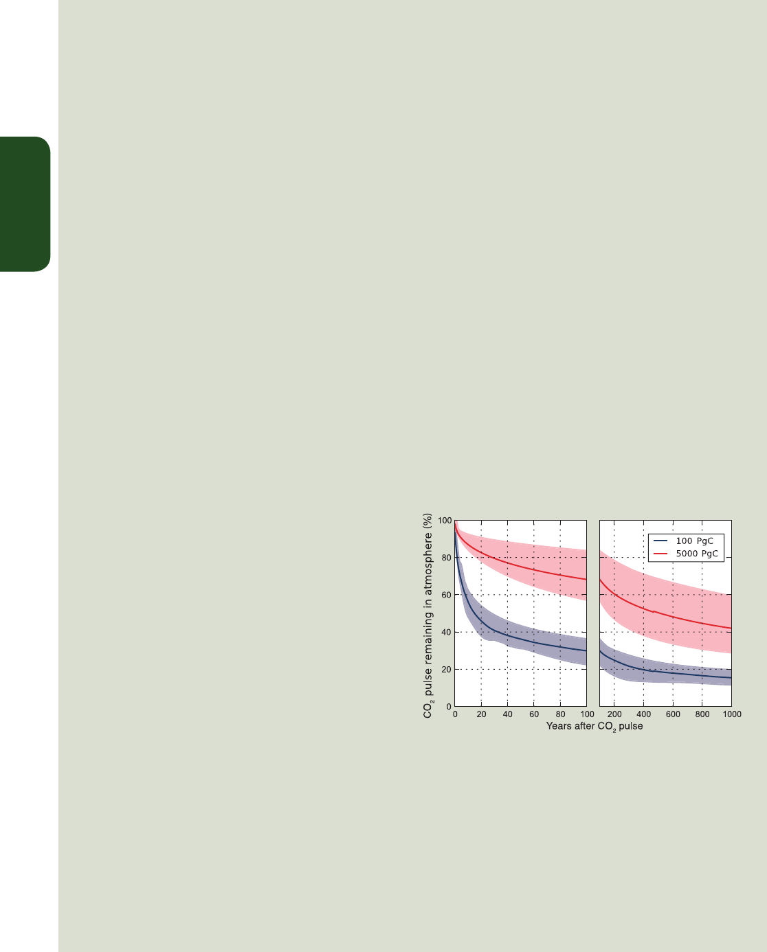
TS
Technical Summary
96
Thematic Focus Elements
TFE.7 | Carbon Cycle Perturbation and Uncertainties
The natural carbon cycle has been perturbed since the beginning of the Industrial Revolution (about 1750) by the
anthropogenic release of carbon dioxide (CO
2
) to the atmosphere, virtually all from fossil fuel combustion and land
use change, with a small contribution from cement production. Fossil fuel burning is a process related to energy
production. Fossil fuel carbon comes from geological deposits of coal, oil and gas that were buried in the Earth crust
for millions of years. Land use change CO
2
emissions are related to the conversion of natural ecosystems into man-
aged ecosystems for food, feed and timber production with CO
2
being emitted from the burning of plant material
or from the decomposition of dead plants and soil organic carbon. For instance when a forest is cleared, the plant
material may be released to the atmosphere quickly through burning or over many years as the dead biomass and
soil carbon decay on their own. {6.1, 6.3; Table 6.1}
The human caused excess of CO
2
in the atmosphere is partly removed from the atmosphere by carbon sinks in land
ecosystems and in the ocean, currently leaving less than half of the CO
2
emissions in the atmosphere. Natural carbon
sinks are due to physical, biological and chemical processes acting on different time scales. An excess of atmospheric
CO
2
supports photosynthetic CO
2
fixation by plants that is stored as plant biomass or in the soil. The residence times
of stored carbon on land depends on the compartments (plant/soil) and composition of the organic carbon, with
time horizons varying from days to centuries. The increased storage in terrestrial ecosystems not affected by land
use change is likely to be caused by enhanced photosynthesis at higher CO
2
levels and nitrogen deposition, and
changes in climate favoring carbon sinks such as longer growing seasons in mid-to-high latitudes. {6.3, 6.3.1}
The uptake of anthropogenic CO
2
by the ocean is primarily a response to increasing CO
2
in the atmosphere. Excess
atmospheric CO
2
absorbed by the surface ocean or transported to the ocean through aquatic systems (e.g., rivers,
groundwaters) gets buried in coastal sediments or transported to deep waters where it is stored for decades to
centuries. The deep ocean carbon can dissolve ocean carbonate sediments to store excess CO
2
on time scales of cen-
turies to millennia. Within a 1 kyr, the remaining atmospheric fraction of the CO
2
emissions will be between 15 and
40%, depending on the amount of carbon released (TFE.7, Figure 1). On geological time scales of 10 kyr or longer,
additional CO
2
is removed very slowly from the atmosphere by rock weathering, pulling the remaining atmospheric
CO
2
fraction down to 10 to 25% after 10 kyr. {Box 6.1}
The carbon cycle response to future climate and CO
2
changes can be viewed as two strong and opposing
feedbacks. The concentration–carbon feedback deter-
mines changes in storage due to elevated CO
2
, and
the climate–carbon feedback determines changes in
carbon storage due to changes in climate. There is
high confidence that increased atmospheric CO
2
will
lead to increased land and ocean carbon uptake but
by an uncertain amount. Models agree on the positive
sign of land and ocean response to rising CO
2
but show
only medium and low agreement for the magnitude
of ocean and land carbon uptake respectively (TFE.7,
Figure 2). Future climate change will decrease land
and ocean carbon uptake compared to the case with
constant climate (medium confidence). This is further
supported by paleoclimate observations and modelling
indicating that there is a positive feedback between cli-
mate and the carbon cycle on century to millennial time
scales. Models agree on the sign, globally negative, of
land and ocean response to climate change but show
low agreement on the magnitude of this response, espe-
cially for the land (TFE.7, Figure 2). A key update since
the IPCC Fourth Assessment Report (AR4) is the introduction of nutrient dynamics in some land carbon models, in
particular the limitations on plant growth imposed by nitrogen availability. There is high confidence that, at the
global scale, relative to the Coupled Model Intercomparison Project Phase 5 (CMIP5) carbon-only Earth System
TFE.7, Figure 1 | Percentage of initial atmospheric CO
2
perturbation remaining
in the atmosphere in response to an idealized instantaneous CO
2
emission pulse
in year 0 as calculated by a range of coupled climate–carbon cycle models. Multi-
model mean (line) and the uncertainty interval (maximum model range, shading)
simulated during 100 years (left) and 1 kyr (right) following the instantaneous
emission pulse of 100 PgC (blue) and 5,000 PgC (red). {Box 6.1, Figure 1}
(continued on next page)

TS
Technical Summary
97
Models (ESMs), CMIP5 ESMs including a land nitrogen cycle will reduce the strength of both the concentration–
carbon feedback and the climate–carbon feedback of land ecosystems (TFE.7, Figure 2). Inclusion of nitrogen-cycle
processes increases the spread across the CMIP5 ensemble. The CMIP5 spread in ocean sensitivity to CO
2
and climate
appears reduced compared to AR4 (TFE.7, Figure 2). {6.2.3, 6.4.2}
With very high confidence, ocean carbon uptake of anthropogenic CO
2
emissions will continue under all four Repre-
sentative Concentration Pathways (RCPs) through to 2100, with higher uptake corresponding to higher concentra-
tion pathways. The future evolution of the land carbon uptake is much more uncertain, with a majority of models
projecting a continued net carbon uptake under all RCPs, but with some models simulating a net loss of carbon by
the land due to the combined effect of climate change and land use change. In view of the large spread of model
results and incomplete process representation, there is low confidence on the magnitude of modelled future land
carbon changes. {6.4.3; Figure 6.24}
Biogeochemical cycles and feedbacks other than the carbon cycle play an important role in the future of the climate
system, although the carbon cycle represents the strongest of these. Changes in the nitrogen cycle, in addition to
interactions with CO
2
sources and sinks, affect emissions of nitrous oxide (N
2
O) both on land and from the ocean.
The human-caused creation of reactive nitrogen has increased steadily over the last two decades and is dominated
by the production of ammonia for fertilizer and industry, with important contributions from legume cultivation
and combustion of fossil fuels. {6.3}
Many processes, however, are not yet represented in coupled climate-biogeochemistry models (e.g., other processes
involving other biogenic elements such as phosphorus, silicon and iron) so their magnitudes have to be estimated in
offline or simpler models, which make their quantitative assessment difficult. It is likely that there will be nonlinear
interactions between many of these processes, but these are not yet well quantified. Therefore any assessment of
the future feedbacks between climate and biogeochemical cycles still contains large uncertainty. {6.4}
TFE.7, Figure 2 | Comparison of carbon cycle feedback metrics between the ensemble of seven General Circulation Models (GCMs) and four Earth System Models of
Intermediate Complexity (EMICs) at the time of AR4 (Coupled Carbon Cycle Climate Model Intercomparison Project (C
4
MIP)) under the SRES A2 scenario and the eight
CMIP5 models under the 140-year 1% CO
2
increase per year scenario. Black dots represent a single model simulation and coloured bars the mean of the multi-model
results, grey dots are used for models with a coupled terrestrial nitrogen cycle. The comparison with C
4
MIP models is for context, but these metrics are known to be
variable across different scenarios and rates of change (see Section 6.4.2). The SRES A2 scenario is closer in rate of change to a 0.5% CO
2
increase per year scenario
and as such it should be expected that the CMIP5 climate–carbon sensitivity terms are comparable, but the concentration–carbon sensitivity terms are likely to be
around 20% smaller for CMIP5 than for C
4
MIP due to lags in the ability of the land and ocean to respond to higher rates of CO
2
increase. This dependence on scenario
reduces confidence in any quantitative statements of how CMIP5 carbon cycle feedbacks differ from C
4
MIP. {Figure 6.21}
0.002 0.004 0.006 0.008
K ppm
-1
0.5 1.0 1.5 2.0 2.5 3.0
PgC ppm
-1
-200 -160 -120 -80 -40 0
PgC K
-1
Climate response
to CO
2
C4MIP
CMIP5
Land C
response to CO
2
Ocean C
response to CO
2
C4MIP
CMIP5
C4MIP
CMIP5
Land C
response to climate
Ocean C
response to climate
C4MIP
CMIP5
C4MIP
CMIP5
TFE.7 (continued)

TS
Technical Summary
98
TS.5.7 Long-term Projections of Sea Level Change
TS.5.7.1 Projections of Global Mean Sea Level Change for
the 21st Century
GMSL rise for 2081–2100 (relative to 1986–2005) for the RCPs will
likely be in the 5 to 95% ranges derived from CMIP5 climate projections
in combination with process-based models of glacier and ice sheet sur-
face mass balance, with possible ice sheet dynamical changes assessed
from the published literature. These likely ranges are 0.26 to 0.55 m
(RCP2.6), 0.32 to 0.63 m (RCP4.5), 0.33 to 0.63 m (RCP6.0) and 0.45
to 0.82 m (RCP8.5) (medium confidence) (Table TS.1, Figure TS.21). For
RCP8.5 the range at 2100 is 0.52 to 0.98 m. The central projections for
GMSL rise in all scenarios lie within a range of 0.05 m until the middle
of the century, when they begin to diverge; by the late 21st century,
they have a spread of 0.25 m. Although RCP4.5 and RCP6.0 are very
similar at the end of the century, RCP4.5 has a greater rate of rise earlier
in the century than RCP6.0. GMSL rise depends on the pathway of CO
2
emissions, not only on the cumulative total; reducing emissions earlier
rather than later, for the same cumulative total, leads to a larger mitiga-
tion of sea level rise. {12.4.1, 13.4.1, 13.5.1; Table 13.5}
Confidence in the projected likely ranges comes from the consistency
of process-based models with observations and physical understand-
ing. The basis for higher projections has been considered and it has
been concluded that there is currently insufficient evidence to evalu-
ate the probability of specific levels above the likely range. Based on
current understanding, only the collapse of marine-based sectors of
the Antarctic ice sheet, if initiated, could cause GMSL to rise substan-
tially above the likely range during the 21st century. There is a lack
of consensus on the probability for such a collapse, and the potential
additional contribution to GMSL rise cannot be precisely quantified,
Box TS.7 | Climate Geoengineering Methods
Geoengineering is defined as the deliberate large-scale intervention in the Earth system to counter undesirable impacts of climate
change on the planet. Carbon Dioxide Reduction (CDR) aims to slow or perhaps reverse projected increases in the future atmospheric
CO
2
concentrations, accelerating the natural removal of atmospheric CO
2
and increasing the storage of carbon in land, ocean and geo-
logical reservoirs. Solar Radiation Management (SRM) aims to counter the warming associated with increasing GHG concentrations by
reducing the amount of sunlight absorbed by the climate system. A related technique seeks to deliberately decrease the greenhouse
effect in the climate system by altering high-level cloudiness. {6.5, 7.7; FAQ 7.3}
CDR methods could provide mitigation of climate change if CO
2
can be reduced, but there are uncertainties, side effects and risks,
and implementation would depend on technological maturity along with economic, political and ethical considerations. CDR would
likely need to be deployed at large-scale and over at least one century to be able to significantly reduce CO
2
concentrations. There are
biogeochemical, and currently technical limitations that make it difficult to provide quantitative estimates of the potential for CDR. It
is virtually certain that CO
2
removals from the atmosphere by CDR would be partially offset by outgassing of CO
2
previously stored
in ocean and terrestrial carbon reservoirs. Some of the climatic and environmental side effects of CDR methods are associated with
altered surface albedo from afforestation, ocean de-oxygenation from ocean fertilization, and enhanced N
2
O emissions. Land-based
CDR methods would probably face competing demands for land. The level of confidence on the effectiveness of CDR methods and their
side effects on carbon and other biogeochemical cycles is low. {6.5; Box 6.2; FAQ 7.3}
SRM remains unimplemented and untested but, if realizable, could offset a global temperature rise and some of its effects. There is
medium confidence that SRM through stratospheric aerosol injection is scalable to counter the RF and some of the climate effects
expected from a twofold increase in CO
2
concentration. There is no consensus on whether a similarly large RF could be achieved from
cloud brightening SRM due to insufficient understanding of aerosol–cloud interactions. It does not appear that land albedo change
SRM could produce a large RF. Limited literature on other SRM methods precludes their assessment. {7.7.2, 7.7.3}
Numerous side effects, risks and shortcomings from SRM have been identified. SRM would produce an inexact compensation for the
RF by GHGs. Several lines of evidence indicate that SRM would produce a small but significant decrease in global precipitation (with
larger differences on regional scales) if the global surface temperature were maintained. Another side effect that is relatively well
characterized is the likelihood of modest polar stratospheric ozone depletion associated with stratospheric aerosol SRM. There could
also be other as yet unanticipated consequences. {7.6.3, 7.7.3, 7.7.4}
As long as GHG concentrations continued to increase, the SRM would require commensurate increase, exacerbating side effects. In
addition, scaling SRM to substantial levels would carry the risk that if the SRM were terminated for any reason, there is high confidence
that surface temperatures would increase rapidly (within a decade or two) to values consistent with the GHG forcing, which would
stress systems sensitive to the rate of climate change. Finally, SRM would not compensate for ocean acidification from increasing CO
2
.
{7.7.3, 7.7.4}

TS
Technical Summary
99
but there is medium confidence that it would not exceed several tenths
of a metre of sea level rise during the 21st century. {13.5.1, 13.5.3}
Under all the RCP scenarios, the time-mean rate of GMSL rise during
the 21st century is very likely to exceed the rate observed during 1971–
2010. In the projections, the rate of rise initially increases. In RCP2.6
it becomes roughly constant (central projection about 4.5 mm yr
–1
)
before the middle of the century, and subsequently declines slightly.
The rate of rise becomes roughly constant in RCP4.5 and RCP6.0 by the
end of the 21st century, whereas acceleration continues throughout
the century in RCP8.5 (reaching 11 [8 to 16] mm yr
–1
during 2081–
2100). {13.5.1; Table 13.5}
In all RCP scenarios, thermal expansion is the largest contribution,
accounting for about 30 to 55% of the total. Glaciers are the next
largest, accounting for 15-35%. By 2100, 15 to 55% of the present
glacier volume is projected to be eliminated under RCP2.6, and 35 to
85% under RCP8.5 (medium confidence). The increase in surface melt-
ing in Greenland is projected to exceed the increase in accumulation,
and there is high confidence that the surface mass balance changes on
the Greenland ice sheet will make a positive contribution to sea level
rise over the 21st century. On the Antarctic ice sheet, surface melting
is projected to remain small, while there is medium confidence that
snowfall will increase (Figure TS.21). {13.3.3, 13.4.3, 13.4.4, 13.5.1;
Table 13.5}
There is medium confidence in the ability to model future rapid chang-
es in ice sheet dynamics on decadal time scales. At the time of the AR4,
scientific understanding was not sufficient to allow an assessment of
the possibility of such changes. Since the publication of the AR4, there
has been substantial progress in understanding the relevant processes
as well as in developing new ice sheet models that are capable of
simulating them. However, the published literature as yet provides only
a partially sufficient basis for making projections related to particular
scenarios. In our projections of GMSL rise by 2081–2100, the likely
range from rapid changes in ice outflow is 0.03 to 0.20 m from the two
ice sheets combined, and its inclusion is the most important reason
why the projections are greater than those given in the AR4. {13.1.5,
13.5.1, 13.5.3}
Semi-empirical models are designed to reproduce the observed sea
level record over their period of calibration, but do not attribute sea
level rise to its individual physical components. For RCPs, some semi-
empirical models project a range that overlaps the process-based likely
range while others project a median and 95-percentile that are about
twice as large as the process-based models. In nearly every case, the
semi-empirical model 95th percentile is higher than the process-based
likely range. For 2081–2100 (relative to 1986–2005) under RCP4.5,
semi-empirical models give median projections in the range 0.56 to
0.97 m, and their 95th percentiles extend to about 1.2 m. This differ-
ence implies either that there is some contribution which is presently
A1B RCP2.6 RCP4.5 RCP6.0 RCP8.5
0.0
0.2
0.4
0.6
0.8
1.0
1.2
Global mean sea level rise (m)
2081-2100 relative to 1986-2005Sum
Thermal expansion
Glaciers
Greenland ice sheet (including dynamical change)
Antarctic ice sheet (including dynamical change)
Land water storage
Greenland ice-sheet rapid dynamical change
Antarctic ice-sheet rapid dynamical change
Figure TS.21 | Projections from process-based models with likely ranges and median values for global mean sea level (GMSL) rise and its contributions in 2081–2100 relative to
1986–2005 for the four RCP scenarios and scenario SRES A1B used in the AR4. The contributions from ice sheets include the contributions from ice sheet rapid dynamical change,
which are also shown separately. The contributions from ice sheet rapid dynamics and anthropogenic land water storage are treated as having uniform probability distributions,
and as independent of scenario (except that a higher rate of change is used for Greenland ice sheet outflow under RCP8.5). This treatment does not imply that the contributions
concerned will not depend on the scenario followed, only that the current state of knowledge does not permit a quantitative assessment of the dependence. See discussion in
Sections 13.5.1 and 13.5.3 and Supplementary Material for methods. Based on current understanding, only the collapse of the marine-based sectors of the Antarctic ice sheet, if
initiated, could cause GMSL to rise substantially above the likely range during the 21st century. This potential additional contribution cannot be precisely quantified but there is
medium confidence that it would not exceed several tenths of a metre during the 21st century. {Figure 13.10}
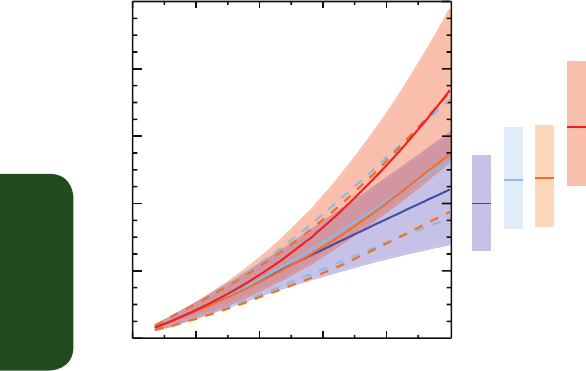
TS
Technical Summary
100
unidentified or underestimated by process-based models, or that the
projections of semi-empirical models are overestimates. Making pro-
jections with a semi-empirical model assumes that sea level change in
the future will have the same relationship as it has had in the past to
RF or global mean temperature change. This may not hold if potentially
nonlinear physical processes do not scale in the future in ways which
can be calibrated from the past. There is no consensus in the scientific
community about the reliability of semi-empirical model projections,
and confidence in them is assessed to be low. {13.5.2, 13.5.3}
TS.5.7.2 Projections of Global Mean Sea Level Change
Beyond 2100
It is virtually certain that GMSL rise will continue beyond 2100. The few
available model results that go beyond 2100 indicate global mean sea
level rise above the pre-industrial level (defined here as an equilibrium
280 ppm atmospheric CO
2
concentration) by 2300 to be less than 1 m
for a RF that corresponds to CO
2
concentrations that peak and decline
and remain below 500 ppm, as in the scenario RCP2.6. For a RF that
corresponds to a CO
2
concentration that is above 700 ppm but below
1500 ppm, as in the scenario RCP8.5, the projected rise is 1 m to more
than 3 m (medium confidence). {13.5.4}
Sea level rise due to ocean thermal expansion will continue for cen-
turies to millennia. The amount of ocean thermal expansion increases
with global warming (models give a range of 0.2 to 0.6 m °C
–1
). The
glacier contribution decreases over time as their volume (currently
about 0.43 m sea level equivalent) decreases. In Antarctica, beyond
2100 and with higher GHG scenarios, the increase in surface melting
could exceed the increase in accumulation. {13.5.2, 13.5.4}
The available evidence indicates that global warming greater than a
certain threshold would lead to the near-complete loss of the Green-
land ice sheet over a millennium or more, causing a GMSL rise of about
7 m. Studies with fixed present-day ice sheet topography indicate the
threshold is greater than 2°C but less than 4°C of GMST rise with
respect to pre-industrial (medium confidence). The one study with a
dynamical ice sheet suggests the threshold is greater than about 1°C
(low confidence) global mean warming with respect to pre-industrial.
Considering the present state of scientific uncertainty, a likely range
cannot be quantified. The complete loss of the ice sheet is not inevi-
table because this would take a millennium or more; if temperatures
decline before the ice sheet is eliminated, the ice sheet might regrow.
However, some part of the mass loss might be irreversible, depending
on the duration and degree of exceedance of the threshold, because
the ice sheet may have multiple steady states, due to its interaction
with its regional climate. {13.4.3, 13.5.4}
Currently available information indicates that the dynamical contribu-
tion of the ice sheets will continue beyond 2100, but confidence in
projections is low. In Greenland, ice outflow induced from interaction
with the ocean is self-limiting as the ice sheet margin retreats inland
from the coast. By contrast, the bedrock topography of Antarctica is
such that there may be enhanced rates of mass loss as the ice retreats.
About 3.3 m of equivalent global sea level of the West Antarctic ice
sheet is grounded on areas with downward sloping bedrock, which
may be subject to potential ice loss via the marine ice sheet instability.
Abrupt and irreversible ice loss from a potential instability of marine-
based sectors of the Antarctic Ice Sheet in response to climate forcing
is possible, but current evidence and understanding is insufficient to
make a quantitative assessment. Due to relatively weak snowfall on
Antarctica and the slow ice motion in its interior, it can be expected
that the West Antarctic ice sheet would take at least several thousand
years to regrow if it was eliminated by dynamic ice discharge. Conse-
quently any significant ice loss from West Antarctic that occurs within
the next century will be irreversible on a multi-centennial to millennial
time scale. {5.8, 13.4.3, 13.4.4, 13.5.4}
TS.5.7.3 Projections of Regional Sea Level Change
Regional sea level will change due to dynamical ocean circulation
changes, changes in the heat content of the ocean, mass redistribution
in the entire Earth system and changes in atmospheric pressure. Ocean
dynamical change results from changes in wind and buoyancy forc-
ing (heat and freshwater), associated changes in the circulation, and
redistribution of heat and freshwater. Over time scales longer than a
few days, regional sea level also adjusts nearly isostatically to regional
changes in sea level atmospheric pressure relative to its mean over
the ocean. Ice sheet mass loss (both contemporary and past), glacier
mass loss and changes in terrestrial hydrology cause water mass redis-
tribution among the cryosphere, the land and the oceans, giving rise
to distinctive regional changes in the solid Earth, Earth rotation and
the gravity field. In some coastal locations, changes in the hydrologi-
cal cycle, ground subsidence associated with anthropogenic activity,
Figure TS.22 | Projections from process-based models of global mean sea level
(GMSL) rise relative to 1986–2005 for the four RCP scenarios. The solid lines show the
median projections, the dashed lines show the likely ranges for RCP4.5 and RCP6.0, and
the shading the likely ranges for RCP2.6 and RCP8.5. The time means for 2081–2100
are shown as coloured vertical bars. See Sections 13.5.1 and 13.5.3 and Supplementary
Material for methods. Based on current understanding, only the collapse of the marine-
based sectors of the Antarctic ice sheet, if initiated, could cause GMSL to rise substan-
tially above the likely range during the 21st century. This potential additional contribu-
tion cannot be precisely quantified but there is medium confidence that it would not
exceed several tenths of a metre during the 21st century. Further detail regarding the
related Figure SPM.9 is given in the TS Supplementary Material. {Table 13.5; Figures
13.10, 13.11}
0.0
0.2
0.4
0.6
0.8
1.0
(m)
2000 2020 2040 2060 2080 2100
Year
RCP2.6
RCP4.5
RCP6.0
RCP8.5
Mean over
2081–2100
Global mean sea level rise
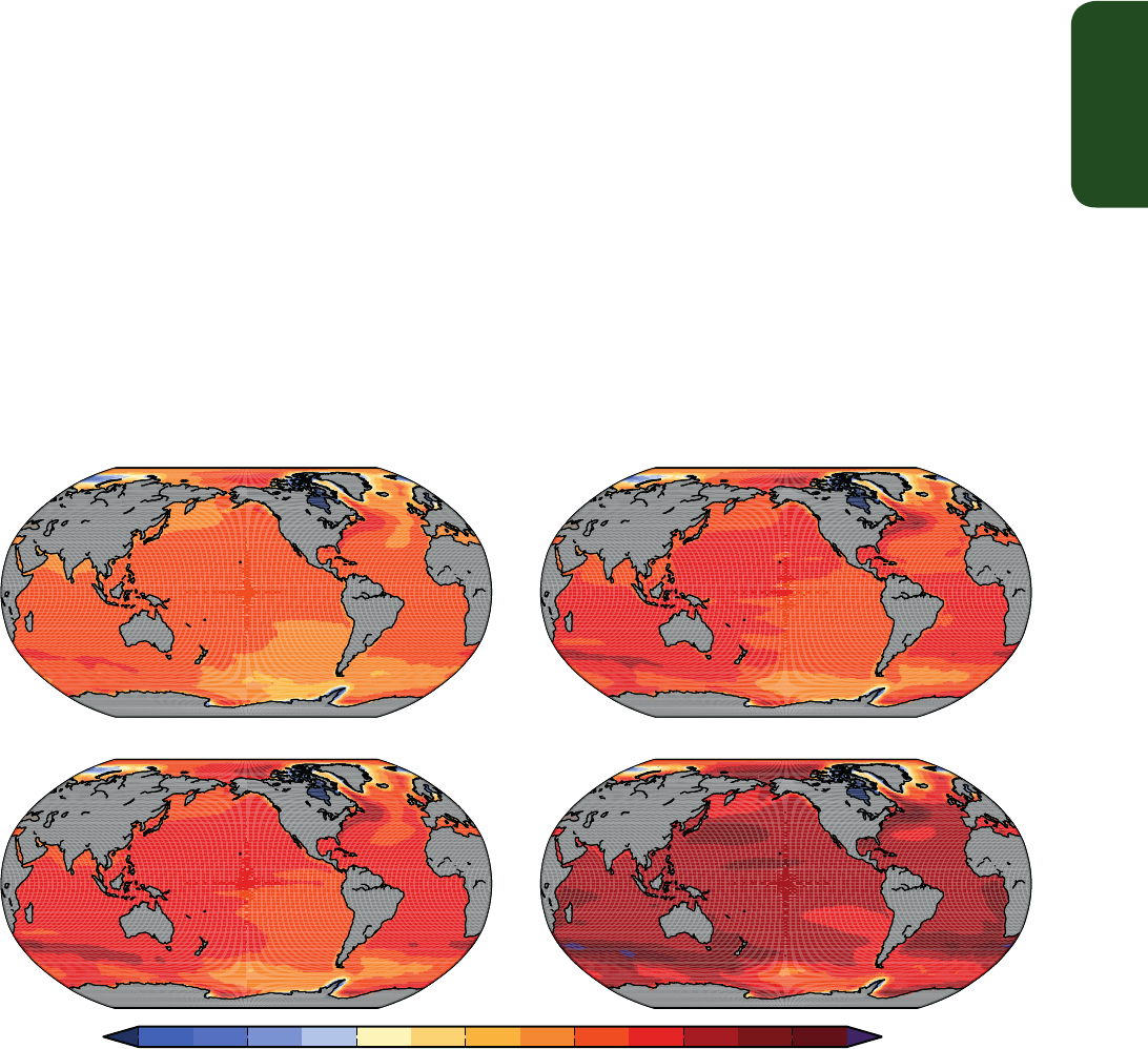
TS
Technical Summary
101
tectonic processes and coastal processes can dominate the relative sea
level change, that is, the change in sea surface height relative to the
land. {13.1.3, 13.6.2, 13.6.3, 13.6.4}
By the end of the 21st century, sea level change will have a strong
regional pattern, which will dominate over variability, with many
regions likely experiencing substantial deviations from the global
mean change (Figure TS.23). It is very likely that over about 95% of
the ocean will experience regional relative sea level rise, while most
regions experiencing a sea level fall are located near current and
former glaciers and ice sheets. Local sea level changes deviate more
than 10% and 25% from the global mean projection for as much as
30% and 9% of the ocean area, respectively, indicating that spatial
variations can be large. Regional changes in sea level reach values of
up to 30% above the global mean value in the Southern Ocean and
around North America, between 10% and 20% in equatorial regions,
and up to 50% below the global mean in the Arctic region and some
regions near Antarctica. About 70% of the coastlines worldwide are
projected to experience a relative sea level change within 20% of the
GMSL change. Over decadal periods, the rates of regional relative sea
level change as a result of climate variability can differ from the global
average rate by more than 100%. {13.6.5}
TS.5.7.4 Projections of Change in Sea Level Extremes and Waves
During the 21st Century
It is very likely that there will be a significant increase in the occurrence
of future sea level extremes by the end of the 21st century, with a likely
increase in the early 21st century (see TFE.9, Table 1). This increase will
primarily be the result of an increase in mean sea level (high confi-
dence), with extreme return periods decreasing by at least an order of
magnitude in some regions by the end of the 21st century. There is low
confidence in region-specific projections of storminess and associated
storm surges. {13.7.2}
It is likely (medium confidence) that annual mean significant wave
heights will increase in the Southern Ocean as a result of enhanced
wind speeds. Southern Ocean–generated swells are likely to affect
heights, periods and directions of waves in adjacent basins. It is very
likely that wave heights and the duration of the wave season will
increase in the Arctic Ocean as a result of reduced sea ice extent. In
general, there is low confidence in region-specific projections due to
the low confidence in tropical and extratropical storm projections, and
to the challenge of down-scaling future wind states from coarse reso-
lution climate models. {13.7.3}
a) b)
c) d)
− 0.4 − 0.2 0.0 0.2 0.4 0.6 0.8
(m)
Relative Sea Level Change 2081-2100 relative to 1986-2005
RCP2.6
RCP6.0 RCP8.5
RCP4.5
Figure TS.23 | Ensemble mean net regional relative sea level change (metres) evaluated from 21 CMIP5 models for the RCP scenarios (a) 2.6, (b) 4.5, (c) 6.0 and (d) 8.5 between
1986–2005 and 2081–2100. Each map includes effects of atmospheric loading, plus land-ice, glacial isostatic adjustment (GIA) and terrestrial water sources. {Figure 13.20}

TS
Technical Summary
102
Thematic Focus Elements
TFE.8 | Climate Targets and Stabilization
The concept of stabilization is strongly linked to the ultimate objective of the United Nations Framework Conven-
tion on Climate Change (UNFCCC), which is ‘to achieve […] stabilization of greenhouse gas concentrations in the
atmosphere at a level that would prevent dangerous anthropogenic interference with the climate system’. Recent
policy discussions focused on limits to a global temperature increase, rather than to greenhouse gas (GHG) con-
centrations, as climate targets in the context of the UNFCCC objectives. The most widely discussed is that of 2°C,
that is, to limit global temperature increase relative to pre-industrial times to below 2°C, but targets other than
2°C have been proposed (e.g., returning warming to well below 1.5°C global warming relative to pre-industrial, or
returning below an atmospheric carbon dioxide (CO
2
) concentration of 350 ppm). Climate targets generally mean
avoiding a warming beyond a predefined threshold. Climate impacts, however, are geographically diverse and
sector specific, and no objective threshold defines when dangerous interference is reached. Some changes may
be delayed or irreversible, and some impacts could be beneficial. It is thus not possible to define a single critical
objective threshold without value judgements and without assumptions on how to aggregate current and future
costs and benefits. This TFE does not advocate or defend any threshold or objective, nor does it judge the economic
or political feasibility of such goals, but assesses, based on the current understanding of climate and carbon cycle
feedbacks, the climate projections following the Representative Concentration Pathways (RCPs) in the context of
climate targets, and the implications of different long-term temperature stabilization objectives on allowed carbon
emissions. Further below it is highlighted that temperature stabilization does not necessarily imply stabilization of
the entire Earth system. {12.5.4}
Temperature targets imply an upper limit on the total radiative forcing (RF). Differences in RF between the four RCP
scenarios are relatively small up to 2030, but become very large by the end of the 21st century and dominated by
CO
2
forcing. Consequently, in the near term, global mean surface temperatures (GMSTs) are projected to continue
to rise at a similar rate for the four RCP scenarios. Around the mid-21st century, the rate of global warming begins
to be more strongly dependent on the scenario. By the end of the 21st century, global mean temperatures will be
warmer than present day under all the RCPs, global temperature change being largest (>0.3°C per decade) in the
highest RCP8.5 and significantly lower in RCP2.6, particularly after about 2050 when global surface temperature
response stabilizes (and declines thereafter) (see Figure TS.15). {11.3.1, 12.3.3, 12.4.1}
In the near term (2016–2035), global mean surface warming is more likely than not to exceed 1°C and very unlikely
to be more than 1.5°C relative to the average from year 1850 to 1900 (assuming 0.61°C warming from 1850-1900
to 1986–2005) (medium confidence). By the end of the 21st century (2081–2100), global mean surface warming,
relative to 1850-1900, is likely to exceed 1.5°C for RCP4.5, RCP6.0 and RCP8.5 (high confidence) and is likely to
exceed 2°C for RCP6.0 and RCP8.5 (high confidence). It is more likely than not to exceed 2°C for RCP4.5 (medium
confidence). Global mean surface warming above 2°C under RCP2.6 is unlikely (medium confidence). Global mean
surface warming above 4°C by 2081–2100 is unlikely in all RCPs (high confidence) except for RCP8.5 where it is about
as likely as not (medium confidence). {11.3.6, 12.4.1; Table 12.3}
Continuing GHG emissions beyond 2100 as in the RCP8.5 extension induces a total RF above 12 W m
–2
by 2300, with
global warming reaching 7.8 [3.0 to 12.6] °C for 2281–2300 relative to 1986–2005. Under the RCP4.5 extension,
where radiative forcing is kept constant (around 4.5 W m
-2
) beyond 2100, global warming reaches 2.5 [1.5 to 3.5]
°C. Global warming reaches 0.6 [0.0 to 1.2] °C under the RCP2.6 extension where sustained negative emissions lead
to a further decrease in RF, reaching values below present-day RF by 2300. See also Box TS.7. {12.3.1, 12.4.1, 12.5.1}
The total amount of anthropogenic CO
2
released in the atmosphere since pre-industrial (often termed cumulative
carbon emission, although it applies only to CO
2
emissions) is a good indicator of the atmospheric CO
2
concentration
and hence of the global warming response. The ratio of GMST change to total cumulative anthropogenic CO
2
emis-
sions is relatively constant over time and independent of the scenario. This near-linear relationship between total CO
2
emissions and global temperature change makes it possible to define a new quantity, the transient climate response
to cumulative carbon emission (TCRE), as the transient GMST change for a given amount of cumulated anthropo-
genic CO
2
emissions, usually 1000 PgC (TFE.8, Figure 1). TCRE is model dependent, as it is a function of the cumulative
CO
2
airborne fraction and the transient climate response, both quantities varying significantly across models. Taking
into account the available information from multiple lines of evidence (observations, models and process under-
standing), the near linear relationship between cumulative CO
2
emissions and peak global mean temperature is
(continued on next page)

TS
Technical Summary
103
well established in the literature and robust for cumulative total CO
2
emissions up to about 2000 PgC. It is consistent
with the relationship inferred from past cumulative CO
2
emissions and observed warming, is supported by process
understanding of the carbon cycle and global energy balance, and emerges as a robust result from the entire hier-
archy of models. Expert judgment based on the available evidence suggests that TCRE is likely between 0.8°C and
2.5°C per 1000 PgC, for cumulative emissions less than about 2000 PgC until the time at which temperature peaks
(TFE.8, Figure 1a). {6.4.3, 12.5.4; Box 12.2}
CO
2
-induced warming is projected to remain approximately constant for many centuries following a complete
cessation of emissions. A large fraction of climate change is thus irreversible on a human time scale, except if net
anthropogenic CO
2
emissions were strongly negative over a sustained period. Based on the assessment of TCRE
(assuming a normal distribution with a ±1 standard deviation range of 0.8 to 2.5°C per 1000 PgC), limiting the
warming caused by anthropogenic CO
2
emissions alone (i.e., ignoring other radiative forcings) to less than 2°C
since the period 1861–1880 with a probability of >33%, >50% and >66%, total CO
2
emissions from all anthropo-
genic sources would need to be below a cumulative budget of about 1570 PgC, 1210 PgC and 1000 PgC since 1870,
respectively. An amount of 515 [445 to 585] PgC was emitted between 1870 and 2011 (TFE.8, Figure 1a,b). Higher
emissions in earlier decades therefore imply lower or even negative emissions later on. Accounting for non-CO
2
forcings contributing to peak warming implies lower cumulated CO
2
emissions. Non-CO
2
forcing constituents are
important, requiring either assumptions on how CO
2
emission reductions are linked to changes in other forcings,
or separate emission budgets and climate modelling for short-lived and long-lived gases. So far, not many studies
have considered non-CO
2
forcings. Those that do consider them found significant effects, in particular warming of
several tenths of a degree for abrupt reductions in emissions of short-lived species, like aerosols. Accounting for an
unanticipated release of GHGs from permafrost or methane hydrates, not included in studies assessed here, would
also reduce the anthropogenic CO
2
emissions compatible with a given temperature target. Requiring a higher likeli-
hood of temperatures remaining below a given temperature target would further reduce the compatible emissions
(TFE.8, Figure 1c). When accounting for the non-CO
2
forcings as in the RCP scenarios, compatible carbon emissions
since 1870 are reduced to about 900 PgC, 820 PgC and 790 PgC to limit warming to less than 2°C since the period
1861–1880 with a probability of >33%, >50%, and >66%, respectively. These estimates were derived by computing
the fraction of the Coupled Model Intercomparison Project Phase 5 (CMIP5) Earth System Models (ESMs) and Earth
System Models of Intermediate Complexity (EMICs) that stay below 2°C for given cumulative emissions following
RCP8.5, as shown in TFE.8 Fig. 1c. The non-CO
2
forcing in RCP8.5 is higher than in RCP2.6. Because all likelihood
statements in calibrated IPCC language are open intervals, the estimates provided are thus both conservative and
consistent choices valid for non-CO
2
forcings across all RCP scenarios. There is no RCP scenario which limits warming
to 2°C with probabilities of >33% or >50%, and which could be used to directly infer compatible cumulative emis-
sions. For a probability of >66% RCP2.6 can be used as a comparison. Combining the average back-calculated fossil
fuel carbon emissions for RCP2.6 between 2012 and 2100 (270 PgC) with the average historical estimate of 515 PgC
gives a total of 785 PgC, i.e., 790 PgC when rounded to 10 PgC. As the 785 PgC estimate excludes an explicit assess-
ment of future land-use change emissions, the 790 PgC value also remains a conservative estimate consistent with
the overall likelihood assessment. The ranges of emissions for these three likelihoods based on the RCP scenarios are
rather narrow, as they are based on a single scenario and on the limited sample of models available (TFE.8 Fig. 1c).
In contrast to TCRE they do not include observational constraints or account for sources of uncertainty not sampled
by the models. The concept of a fixed cumulative CO
2
budget holds not just for 2°C, but for any temperature level
explored with models so far (up to about 5°C, see Figures 12.44 to 12.46). Higher temperature targets would allow
larger cumulative budgets, while lower temperature target would require lower cumulative budgets (TFE.8, Figure
1). {6.3.1, 12.5.2, 12.5.4}
The climate system has multiple time scales, ranging from annual to multi-millennial, associated with different
thermal and carbon reservoirs. These long time scales induce a commitment warming ‘already in the pipe-line’.
Stabilization of the forcing would not lead to an instantaneous stabilization of the warming. For the RCP scenarios
and their extensions to 2300, the fraction of realized warming, at that time when RF stabilizes, would be about 75
to 85% of the equilibrium warming. For a 1% yr
–1
CO
2
increase to 2 × CO
2
or 4 × CO
2
and constant forcing there-
after, the fraction of realized warming would be much smaller, about 40 to 70% at the time when the forcing is
kept constant. Owing to the long time scales in the deep ocean, full equilibrium is reached only after hundreds to
thousands of years. {12.5.4}
TFE.8 (continued)
(continued on next page)
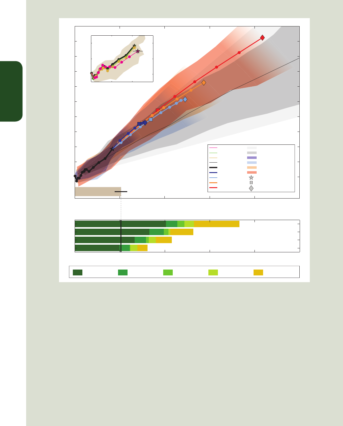
TS
Technical Summary
104
TFE.8, Figure 1 | Global mean temperature increase since 1861–1880 as a function of cumulative total global CO
2
emissions from various lines of evidence. (a)
Decadal average results are shown over all CMIP5 Earth System Model of Intermediate Complexity (EMICs) and Earth System Models (ESMs) for each RCP respectively,
with coloured lines (multi-model average), decadal markers (dots) and with three decades (2000–2009, 2040–2049 and 2090–2099) highlighted with a star, square
and diamond, respectively. The historical time period up to decade 2000–2009 is taken from the CMIP5 historical runs prolonged by RCP8.5 for 2006–2010 and is
indicated with a black thick line and black symbols. Coloured ranges illustrate the model spread (90% range) over all CMIP5 ESMs and EMICs and do not represent
a formal uncertainty assessment. Ranges are filled as long as data of all models is available and until peak temperature. They are faded out for illustrative purposes
afterward. CMIP5 simulations with 1% yr
–1
CO
2
increase only are illustrated by the dark grey area (range definition similar to RCPs above) and the black thin line (multi-
model average). The light grey cone represents this Report’s assessment of the transient climate response to emissions (TCRE) from CO
2
only. Estimated cumulative
historical CO
2
emissions from 1870 to 2011 with associated uncertainties are illustrated by the grey bar at the bottom of (a). (b) Comparison of historical model results
with observations. The magenta line and uncertainty ranges are based on observed emissions from Carbon Dioxide Information Analysis Center (CDIAC) extended by
values of the Global Carbon project until 2010 and observed temperature estimates of the Hadley Centre/Climatic Research Unit gridded surface temperature data set
4 (HadCRUT4). The uncertainties in the last decade of observations are based on the assessment in this report. The black thick line is identical to the one in (a). The
thin green line with crosses is as the black line but for ESMs only. The yellow-brown line and range show these ESM results until 2010, when corrected for HadCRUT4’s
incomplete geographical coverage over time. All values are given relative to the 1861–1880 base period. All time-series are derived from decadal averages to illustrate
the long-term trends. Note that observations are in addition subject to internal climate variability, adding an uncertainty of about 0.1°C. (c) Cumulative CO
2
emis-
sions over the entire industrial era, consistent with four illustrative peak global temperature limits (1.5°C, 2°C, 2.5°C and 3°C, respectively) when taking into account
warming by all forcers. Horizontal bars indicate consistent cumulative emission budgets as a function of the fraction of models (CMIP5 ESMs and EMICs) that at least
hold warming below a given temperature limit. Note that the fraction of models cannot be interpreted as a probability. The budgets are derived from the RCP8.5 runs,
with relative high non-CO
2
forcing over the 21st century. If non-CO
2
are significantly reduced, the CO
2
emissions compatible with a specific temperature limit might
be slightly higher, but only to a very limited degree, as illustrated by the other coloured lines in (a), which assume significantly lower non-CO
2
forcing. Further detail
regarding the related Figure SPM.10 is given in the TS Supplementary Material. {Figure 12.45}
0 500 1000 1500 2000 2500
0
1
2
3
4
5
Cumulative total anthropogenic
CO
2
emissions from 1870 (PgC)
Temperature anomaly relative to 1861-1880 (°C)
RCP2.6
Historical
1% CO
2
runs
Observations
CMIP5 ESM
Masked ESM
RCP4.5
RCP6.0
RCP8.5
RCP8.5 range
RCP6 range
RCP4.5 range
2040-2049 average
2000-2009 average
2090-2099 average
RCP2.6 range
1% CO
2
runs
TCRE assessment
0 500 1000 1500 2000 2500
1.5
2
2.5
3
Consistent cum. total anthropogenic CO
2
emissions given warming by all forcers in RCP8.5 (PgC)
Peak warming limit (°C)
90% of models 66% of models
50% of models 33% of models 10% of models
c
a
Cumulative emissions
estimate 1870-2011
0 200 400 600
0
0.5
1
b
TFE.8 (continued)

TS
Technical Summary
105
The commitment to past emissions is a persistent warming for hundreds of years, continuing at about the level of
warming that has been realized when emissions were ceased. The persistence of this CO
2
-induced warming after
emission have ceased results from a compensation between the delayed commitment warming described above
and the slow reduction in atmospheric CO
2
resulting from ocean and land carbon uptake. This persistence of warm-
ing also results from the nonlinear dependence of RF on atmospheric CO
2
, that is, the relative decrease in forcing
being smaller than the relative decrease in CO
2
concentration. For high climate sensitivities, and in particular if
sulphate aerosol emissions are eliminated at the same time as GHG emissions, the commitment from past emission
can be strongly positive, and is a superposition of a fast response to reduced aerosols emissions and a slow response
to reduced CO
2
. {12.5.4}
Stabilization of global temperature does not imply stabilization for all aspects of the climate system. Processes
related to vegetation change, changes in the ice sheets, deep ocean warming and associated sea level rise and
potential feedbacks linking, for example, ocean and the ice sheets have their own intrinsic long time scales. Ocean
acidification will very likely continue in the future as long as the oceans will continue to take up atmospheric CO
2
.
Committed land ecosystem carbon cycle changes will manifest themselves further beyond the end of the 21st
century. It is virtually certain that global mean sea level rise will continue beyond 2100, with sea level rise due to
thermal expansion to continue for centuries to millennia. Global mean sea level rise depends on the pathway of CO
2
emissions, not only on the cumulative total; reducing emissions earlier rather than later, for the same cumulative
total, leads to a larger mitigation of sea level rise. {6.4.4, 12.5.4, 13.5.4}
TFE.8 (continued)
TS.5.8 Climate Phenomena and Regional Climate Change
This section assesses projected changes over the 21st century in large-
scale climate phenomena that affect regional climate (Table TS.2).
Some of these phenomena are defined by climatology (e.g., mon-
soons), and some by interannual variability (e.g., El Niño), the latter
affecting climate extremes such as floods, droughts and heat waves.
Changes in statistics of weather phenomena such as tropical cyclones
and extratropical storms are also summarized here. {14.8}
TS.5.8.1 Monsoon Systems
Global measures of monsoon by the area and summer precipitation are
likely to increase in the 21st century, while the monsoon circulation
weakens. Monsoon onset dates are likely to become earlier or not to
change much while monsoon withdrawal dates are likely to delay, result-
ing in a lengthening of the monsoon season in many regions (Figure
TS.24). The increase in seasonal mean precipitation is pronounced in
the East and South Asian summer monsoons while the change in other
monsoon regions is subject to larger uncertainties. {14.2.1}
There is medium confidence that monsoon-related interannual rainfall
variability will increase in the future. Future increase in precipitation
extremes related to the monsoon is very likely in South America, Africa,
East Asia, South Asia, Southeast Asia and Australia. {14.2.1, 14.8.5,
14.8.7, 14.8.9, 14.8.11–14.8.13}
There is medium confidence that overall precipitation associated with
the Asian-Australian monsoon will increase but with a north–south
asymmetry: Indian monsoon rainfall is projected to increase, while
projected changes in the Australian summer monsoon rainfall are
small. There is medium confidence in that the Indian summer monsoon
circulation weakens, but this is compensated by increased atmospheric
moisture content, leading to more rainfall. For the East Asian summer
monsoon, both monsoon circulation and rainfall are projected to
increase. {14.2.2, 14.8.9, 14.8.11, 14.8.13}
There is low confidence in projections of the North American and South
American monsoon precipitation changes, but medium confidence that
the North American monsoon will arrive and persist later in the annual
cycle, and high confidence in expansion of South American Monsoon
area. {14.2.3, 14.8.3–14.8.5}
There is low confidence in projections of a small delay in the West
African rainy season, with an intensification of late-season rains. The
limited skills of model simulations for the region suggest low confi-
dence in the projections. {14.2.4, 14.8.7}
TS.5.8.2 Tropical Phenomena
Precipitation change varies in space, increasing in some regions and
decreasing in some others. The spatial distribution of tropical rainfall
changes is likely shaped by the current climatology and ocean warm-
ing pattern. The first effect is to increase rainfall near the currently
rainy regions, and the second effect increases rainfall where the ocean
warming exceeds the tropical mean. There is medium confidence that
tropical rainfall projections are more reliable for the seasonal than
annual mean changes. {7.6.2, 12.4.5, 14.3.1}
There is medium confidence in future increase in seasonal mean pre-
cipitation on the equatorial flank of the Intertropical Convergence
Zone and a decrease in precipitation in the subtropics including parts

TS
Technical Summary
106
Regions Projected Major Changes in Relation to Phenomena
Arctic
{14.8.2}
Wintertime changes in temperature and precipitation resulting from the small projected increase in North Atlantic Oscillation (NAO); enhanced warming
and sea ice melting; significant increase in precipitation by mid-century due mostly to enhanced precipitation in extratropical cyclones.
North America
{14.8.3}
Monsoon precipitation will shift later in the annual cycle; increased precipitation in extratropical cyclones will lead to large increases in wintertime
precipitation over the northern third of the continent; extreme precipitation increases in tropical cyclones making landfall along the western coast of
USA and Mexico, the Gulf Mexico, and the eastern coast of USA and Canada.
Central America and Caribbean
{14.8.4}
Projected reduction in mean precipitation and increase in extreme precipitation; more extreme precipitation in tropical cyclones making landfall along
the eastern and western coasts.
South America
{14.8.5}
A southward displaced South Atlantic Convergence Zone increases precipitation in the southeast; positive trend in the Southern Annular Mode displaces
the extratropical storm track southward, decreasing precipitation in central Chile and increasing it at the southern tip of South America.
Europe and Mediterranean
{14.8.6}
Enhanced extremes of storm-related precipitation and decreased frequency of storm-related precipitation over the eastern Mediterranean.
Africa
{14.8.7}
Enhanced summer monsoon precipitation in West Africa; increased short rain in East Africa due to the pattern of Indian Ocean warming; increased
rainfall extremes of landfall cyclones on the east coast (including Madagascar).
Central and North Asia
{14.8.8}
Enhanced summer precipitation; enhanced winter warming over North Asia.
East Asia
{14.8.9}
Enhanced summer monsoon precipitation; increased rainfall extremes of landfall typhoons on the coast; reduction in the midwinter suppression of
extratropical cyclones.
West Asia
{14.8.10}
Increased rainfall extremes of landfall cyclones on the Arabian Peninsula; decreased precipitation in northwest Asia due to a northward shift of extra-
tropical storm tracks.
South Asia
{14.8.11}
Enhanced summer monsoon precipitation; increased rainfall extremes of landfall cyclones on the coasts of the Bay of Bengal and Arabian Sea.
Southeast Asia
{14.8.12}
Reduced precipitation in Indonesia during July to October due to the pattern of Indian Ocean warming; increased rainfall extremes of landfall cyclones
on the coasts of the South China Sea, Gulf of Thailand and Andaman Sea.
Australia and New Zealand
{14.8.13}
Summer monsoon precipitation may increase over northern Australia; more frequent episodes of the zonal South Pacific Convergence Zone may reduce
precipitation in northeastern Australia; increased warming and reduced precipitation in New Zealand and southern Australia due to projected positive
trend in the Southern Annular Mode; increased extreme precipitation associated with tropical and extratropical storms
Pacific Islands
{14.8.14}
Tropical convergence zone changes affect rainfall and its extremes; more extreme precipitation associated with tropical cyclones
Antarctica
{14.8.15}
Increased warming over Antarctic Peninsula and West Antarctic related to the positive trend in the Southern Annular Mode; increased precipitation in
coastal areas due to a poleward shift of storm track.
Table TS.2 | Overview of projected regional changes and their relation to major climate phenomena. A phenomenon is considered relevant when there is both sufficient confidence
that it has an influence on the given region, and when there is sufficient confidence that the phenomenon will change, particularly under the RCP4.5 or higher end scenarios. See
Section 14.8 and Tables 14.2 and 14.3 for full assessment of the confidence in these changes, and their relevance for regional climate. {14.8; Tables 14.2, 14.3}
of North and Central Americas, the Caribbean, South America, Africa
and West Asia. There is medium confidence that the interannual occur-
rence of zonally oriented South Pacific Convergence Zone events will
increase, leading possibly to more frequent droughts in the southwest
Pacific. There is medium confidence that the South Atlantic Conver-
gence Zone will shift southwards, leading to a precipitation increase
over southeastern South America and a reduction immediately north
of the convergence zone. {14.3.1, 14.8.3–14.8.5, 14.8.7, 14.8.11,
14.8.14}
The tropical Indian Ocean is likely to feature a zonal pattern with
reduced warming and decreased rainfall in the east (including Indone-
sia), and enhanced warming and increased rainfall in the west (includ-
ing East Africa). The Indian Ocean dipole mode of interannual variabil-
ity is very likely to remain active, affecting climate extremes in East
Africa, Indonesia and Australia. {14.3.3, 14.8.7, 14.8.12}
There is low confidence in the projections for the tropical Atlantic—
both for the mean and interannual modes, because of large errors in
model simulations in the region. Future projections in Atlantic hurri-
canes and tropical South American and West African precipitation are
therefore of low confidence. {14.3.4, 14.6.1, 14.8.5,14.8.7}
It is currently not possible to assess how the Madden–Julian Oscilla-
tion will change owing to the poor skill in model simulations of this
intraseasonal phenomenon and the sensitivity to ocean warming pat-
terns. Future projections of regional climate extremes in West Asia,
Southeast Asia and Australia are therefore of low confidence. {9.5.2,
14.3.4, 14.8.10, 14.8.12, 14.8.13}
TS.5.8.3 El Niño-Southern Oscillation
There is high confidence that the El Niño-Southern Oscillation (ENSO)
will remain the dominant mode of natural climate variability in the
21st century with global influences in the 21st century, and that
regional rainfall variability it induces likely intensifies. Natural varia-
tions of the amplitude and spatial pattern of ENSO are so large that
confidence in any projected change for the 21st century remains low.
The projected change in El Niño amplitude is small for both RCP4.5 and
RCP8.5 compared to the spread of the change among models (Figure
TS.25). Over the North Pacific and North America, patterns of tempera-
ture and precipitation anomalies related to El Niño and La Niña (tele-
connections) are likely to move eastwards in the future (medium confi-
dence), while confidence is low in changes in climate impacts on other
regions including Central and South Americas, the Caribbean, Africa,
most of Asia, Australia and most Pacific Islands. In a warmer climate,
the increase in atmospheric moisture intensifies temporal variability

TS
Technical Summary
107
Figure TS.24 | Future change in monsoon statistics between the present-day (1986–2005) and the future (2080–2099) based on CMIP5 ensemble from RCP2.6 (dark blue; 18
models), RCP4.5 (blue; 24), RCP6.0 (yellow; 14), and RCP8.5 (red; 26) simulations. (a) GLOBAL: Global monsoon area (GMA), global monsoon intensity (GMI), standard deviation
of inter-annual variability in seasonal precipitation (Psd), seasonal maximum 5-day precipitation total (R5d) and monsoon season duration (DUR). Regional land monsoon domains
determined by 24 multi-model mean precipitation in the present-day. (b)–(h) Future change in regional land monsoon statistics: seasonal average precipitation (Pav), Psd, R5d, and
DUR in (b) North America (NAMS), (c) North Africa (NAF), (d) South Asia (SAS), (e) East Asia (EAS), (f) Australia-Maritime continent (AUSMC), (g) South Africa (SAF) and (h) South
America (SAMS). Units are % except for DUR (days). Box-and-whisker plots show the 10th, 25th, 50th, 75th and 90th percentiles. All the indices are calculated for the summer
season (May to September for the Northern, and November to March for the Southern Hemisphere) over each model’s monsoon domains. {Figures 14.3, 14.4, 14.6, 14.7}
of precipitation even if atmospheric circulation variability remains the
same. This applies to ENSO-induced precipitation variability but the
possibility of changes in ENSO teleconnections complicates this gener-
al conclusion, making it somewhat regional-dependent. {12.4.5, 14.4,
14.8.3–14.8.5, 14.8.7, 14.8.9, 14.8.11–14.8.14}
TS.5.8.4 Cyclones
Projections for the 21st century indicate that it is likely that the global
frequency of tropical cyclones will either decrease or remain essentially
unchanged, concurrent with a likely increase in both global mean trop-
ical cyclone maximum wind speed and rain rates (Figure TS.26). The
influence of future climate change on tropical cyclones is likely to vary
by region, but there is low confidence in region-specific projections.
The frequency of the most intense storms will more likely than not
increase in some basins. More extreme precipitation near the centers
of tropical cyclones making landfall is projected in North and Central
America, East Africa, West, East, South and Southeast Asia as well as
in Australia and many Pacific islands (medium confidence). {14.6.1,
14.8.3, 14.8.4, 14.8.7, 14.8.9–14.8.14}
40 N
60 W0 60 E 120 E 180
20 N
EQ
20 S
40 S
NAMS
SAF
SAS
EAS
NAF
AUSMC
SAMS
Regional land monsoon domain
120 W
90 % tile
75 % tile
50 % tile
25 % tile
10 % tile
60
40
0
-20
-40
-60
20
Pav Psd R5d DUR
(e) EAS
60
40
0
-20
-40
-60
20
Pav Psd R5d DUR
(f) AUSMC
(a) GLOBAL
40
20
0
-20
GMA
GMI
Psd R5d DUR
60
40
0
-20
-40
-60
20
Pav Psd R5d DUR
(b) NAMS
Change (% or days)
60
40
0
-20
-40
-60
20
Pav Psd R5d DUR
(c) NAF
60
40
0
-20
-40
-60
20
Pav Psd R5d DUR
(d) SAS
60
40
0
-20
-40
-60
20
Pav Psd R5d DUR
(h) SAMS
60
40
0
-20
-40
-60
20
Pav Psd R5d DUR
(g) SAF
Standard deviation of Nino3 index (°C)
1.2
1
0.8
0.6
0.4
PI 20C RCP4.5 RCP8.5
Figure TS.25 | Standard deviation in CMIP5 multi-model ensembles of sea surface
temperature variability over the eastern equatorial Pacific Ocean (Nino3 region: 5°S to
5°N, 150°W to 90°W), a measure of El Niño amplitude, for the pre-industrial (PI) control
and 20th century (20C) simulations, and 21st century projections using RCP4.5 and
RCP8.5. Open circles indicate multi-model ensemble means, and the red cross symbol is
the observed standard deviation for the 20th century. Box-and-whisker plots show the
16th, 25th, 50th, 75th and 84th percentiles. {Figure 14.14}
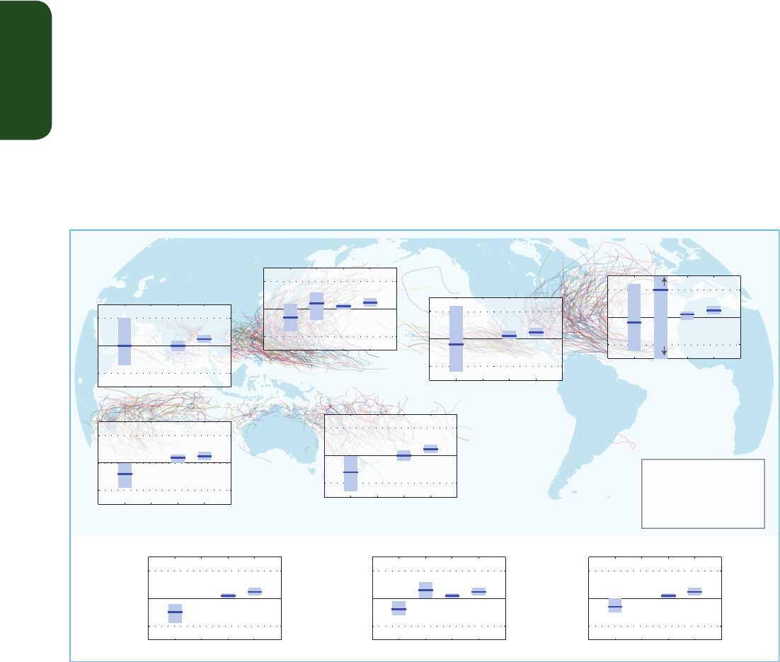
TS
Technical Summary
108
The global number of extratropical cyclones is unlikely to decrease by
more than a few percent and future changes in storms are likely to
be small compared to natural interannual variability and substantial
variations between models. A small poleward shift is likely in the SH
storm track but the magnitude of this change is model dependent. It is
unlikely that the response of the North Atlantic storm track in climate
projections is a simple poleward shift. There is medium confidence in a
projected poleward shift in the North Pacific storm track. There is low
confidence in the impact of storm track changes on regional climate
at the surface. More precipitation in extratropical cyclones leads to a
winter precipitation increase in Arctic, Northern Europe, North America
and the mid-to-high-latitude SH. {11.3.2, 12.4.4, 14.6.2, 14.8.2, 14.8.3,
14.8.5, 14.8.6, 14.8.13, 14.8.15}
TS.5.8.5 Annular and Dipolar Modes of Variability
Future boreal wintertime North Atlantic Oscillation (NAO is very likely
to exhibit large natural variations as observed in the past. The NAO is
likely to become slightly more positive (on average), with some, but not
very well documented implications for winter conditions in the Arctic,
Tropical Cyclone (TC) Metrics:
I All TC frequency
II Category 4-5 TC frequency
III Lifetime Maximum Intensity
IV Precipitation rate
insf. d.insf. d.
I II IIII IV
−50
0
50
% Change
North Indian
insf. d.
I II IIII IV
−50
0
50
% Change
Eastern North Pacific
insf. d.
I II IIII IV
−50
0
50
% Change
South Indian
insf. d.
I II IIII IV
−50
0
50
% Change
Western North Pacific
I II IIII IV
−50
0
50
% Change
South Pacific
insf. d.
I II IIII IV
−50
0
50
% Change
North Atlantic
200 %
-100 %
I II IIII IV
−50
0
50
% Change
GLOBAL
I II IIII IV
−50
0
50
% Change
SOUTHERN HEMISPHERE
insf. d.
I II IIII IV
−50
0
50
% Change
NORTHERN HEMISPHERE
insf. d.
Figure TS.26 | Projected changes in tropical cyclone statistics. All values represent expected percent change in the average over period 2081–2100 relative to 2000–2019, under
an A1B-like scenario, based on expert judgement after subjective normalization of the model projections. Four metrics were considered: the percent change in I) the total annual
frequency of tropical storms, II) the annual frequency of Category 4 and 5 storms, III) the mean Lifetime Maximum Intensity (LMI; the maximum intensity achieved during a storm’s
lifetime) and IV) the precipitation rate within 200 km of storm center at the time of LMI. For each metric plotted, the solid blue line is the best guess of the expected percent change,
and the coloured bar provides the 67% (likely) confidence interval for this value (note that this interval ranges across –100% to +200% for the annual frequency of Category 4
and 5 storms in the North Atlantic). Where a metric is not plotted, there are insufficient data (denoted X) available to complete an assessment. A randomly drawn (and coloured)
selection of historical storm tracks are underlaid to identify regions of tropical cyclone activity. See Section 14.6.1 for details. {14.6.1}
North America and Eurasia. The austral summer/autumn positive trend
in Southern Annular Mode (SAM) is likely to weaken considerably as
stratospheric ozone recovers through the mid-21st century with some,
but not very well documented, implications for South America, Africa,
Australia, New Zealand and Antarctica. {11.3.2, 14.5.2,14.8.5, 14.8.7,
14.8.13, 14.8.15}
TS.5.8.6 Additional Phenomena
It is unlikely that the Atlantic Multi-decadal Oscillation (AMO will
change its behaviour as the mean climate changes. However, natural
fluctuations in the AMO over the coming few decades are likely to
influence regional climates at least as strongly as will human-induced
changes with implications for Atlantic major hurricane frequency, the
West African monsoon and North American and European summer con-
ditions. {14.2.4, 14.5.1, 14.6.1, 14.7.6, 14.8.2, 14.8.3, 14.8.6, 14.8.8}
There is medium confidence that the frequency of NH and SH blocking
will not increase, while the trends in blocking intensity and persistence
remain uncertain. {Box 14.2}

TS
Technical Summary
109
Thematic Focus Elements
TFE.9 | Climate Extremes
Assessing changes in climate extremes poses unique challenges, not just because of the intrinsically rare nature
of these events, but because they invariably happen in conjunction with disruptive conditions. They are strongly
influenced by both small- and large-scale weather patterns, modes of variability, thermodynamic processes, land–
atmosphere feedbacks and antecedent conditions. Much progress has been made since the IPCC Fourth Assessment
Report (AR4) including the comprehensive assessment of extremes undertaken by the IPCC Special Report on Man-
aging the Risk of Extreme Events and Disasters to Advance Climate Change Adaptation (SREX) but also because of
the amount of observational evidence available, improvements in our understanding and the ability of models to
simulate extremes. {1.3.3, 2.6, 7.6, 9.5.4}
For some climate extremes such as droughts, floods and heat waves, several factors need to be combined to produce
an extreme event. Analyses of rarer extremes such as 1-in-20- to 1-in-100-year events using Extreme Value Theory
are making their way into a growing body of literature. Other recent advances concern the notion of ‘fraction of
attributable risk’ that aims to link a particular extreme event to specific causal relationships. {1.3.3, 2.6.1, 2.6.2,
10.6.2, 12.4.3; Box 2.4}
TFE.9, Table 1 indicates the changes that have been observed in a range of weather and climate extremes over the
last 50 years, the assessment of the human contribution to those changes, and how those extremes are expected
to change in the future. The table also compares the current assessment with that of the AR4 and the SREX where
applicable. {2.6, 3.7, 10.6, 11.3, 12.4, 14.6}
Temperature Extremes, Heat Waves and Warm Spells
It is very likely that both maximum and minimum temperature extremes have warmed over most land areas since
the mid-20th century. These changes are well simulated by current climate models, and it is very likely that anthro-
pogenic forcing has affected the frequency of these extremes and virtually certain that further changes will occur.
This supports AR4 and SREX conclusions although with greater confidence in the anthropogenic forcing compo-
nent. {2.6.1, 9.5.4, 10.6.1, 12.4.3}
For land areas with sufficient data there has been an overall increase in the number of warm days and nights. Simi-
lar decreases are seen in the number of cold days and nights. It is very likely that increases in unusually warm days
and nights and/or reductions in unusually cold days and nights including frosts have occurred over this period across
most continents. Warm spells or heat waves containing consecutive extremely hot days or nights are often associ-
ated with quasi-stationary anticyclonic circulation anomalies and are also affected by pre-existing soil conditions
and the persistence of soil moisture anomalies that can amplify or dampen heat waves particularly in moisture-
limited regions. Most global land areas, with a few exceptions, have experienced more heat waves since the middle
of the 20th century. Several studies suggest that increases in mean temperature account for most of the changes
in heat wave frequency, however, heat wave intensity/amplitude is highly sensitive to changes in temperature vari-
ability and the shape of the temperature distribution and heat wave definition also plays a role. Although in some
regions instrumental periods prior to the 1950s had more heat waves (e.g., USA), for other regions such as Europe,
an increase in heat wave frequency in the period since the 1950s stands out in long historical temperature series.
{2.6, 2.6.1, 5.5.1; Box 2.4; Tables 2.12, 2.13; FAQ 2.2}
The observed features of temperature extremes and heat waves are well simulated by climate models and are simi-
lar to the spread among observationally based estimates in most regions. Regional downscaling now offers cred-
ible information on the spatial scales required for assessing extremes and improvements in the simulation of the
El Niño-Southern Oscillation from Coupled Model Intercomparison Project Phase 3 (CMIP3) to Phase 5 (CMIP5) and
other large-scale phenomena is crucial. However simulated changes in frequency and intensity of extreme events
is limited by observed data availability and quality issues and by the ability of models to reliably simulate certain
feedbacks and mean changes in key features of circulation such as blocking. {2.6, 2.7, 9.4, 9.5.3, 9.5.4, 9.6, 9.6.1,
10.3, 10.6, 14.4; Box 14.2}
Since AR4, the understanding of mechanisms and feedbacks leading to changes in extremes has improved. There
continues to be strengthening evidence for a human influence on the observed frequency of extreme temperatures
and heat waves in some regions. Near-term (decadal) projections suggest likely increases in temperature extremes
but with little distinguishable separation between emissions scenarios (TFE.9, Figure 1). Changes may proceed at
(continued on next page)

TS
Technical Summary
110
Phenomenon and
direction of trend
Assessment that changes occurred (typically
since 1950 unless otherwise indicated)
Assessment of a human
contribution to observed changes
Early 21st century Late 21st century
Warmer and/or fewer
cold days and nights
over most land areas
Very likely {2.6}
Very likely
Very likely
Very likely {10.6}
Likely
Likely
Likely {11.3} Virtually certain {12.4}
Virtually certain
Virtually certain
Warmer and/or more
frequent hot days and
nights over most land areas
Very likely {2.6}
Very likely
Very likely
Very likely {10.6}
Likely
Likely (nights only)
Likely {11.3} Virtually certain {12.4}
Virtually certain
Virtually certain
Warm spells/heat waves.
Frequency and/or duration
increases over most
land areas
Medium confidence on a global scale
Likely in large parts of Europe, Asia and Australia {2.6}
Medium confidence in many (but not all) regions
Likely
Likely
a
{10.6}
Not formally assessed
More likely than not
Not formally assessed
b
{11.3}
Very likely {12.4}
Very likely
Very likely
Heavy precipitation events.
Increase in the frequency,
intensity, and/or amount
of heavy precipitation
Likely more land areas with increases than decreases
c
{2.6}
Likely more land areas with increases than decreases
Likely over most land areas
Medium confidence
{7.6, 10.6}
Medium confidence
More likely than not
Likely over many land areas
{11.3}
Very likely over most of the mid-latitude land
masses and over wet tropical regions {12.4}
Likely over many areas
Very likely over most land areas
Increases in intensity
and/or duration of drought
Low confidence on a global scale
Likely changes in some regions
d
{2.6}
Medium confidence in some regions
Likely in many regions, since 1970
e
Low confidence {10.6}
Medium confidence
f
More likely than not
Low confidence
g
{11.3} Likely (medium confidence) on a regional to
global scale
h
{12.4}
Medium confidence in some regions
Likely
e
Increases in intense
tropical cyclone activity
Low confidence in long term (centennial) changes
Virtually certain in North Atlantic since 1970
{2.6}
Low confidence
Likely in some regions, since 1970
Low confidence
i
{10.6}
Low confidence
More likely than not
Low confidence
{11.3}
More likely than not in the Western North Pacific
and North Atlantic
j
{14.6}
More likely than not in some basins
Likely
Increased incidence and/or
magnitude of extreme
high sea level
Likely (since 1970) {3.7}
Likely (late 20th century)
Likely
Likely
k
{3.7}
Likely
k
More likely than not
k
Likely
l
{13.7} Very likely
l
{13.7}
Very likely
m
Likely
Likelihood of further changes
TFE.9, Table 1 | Extreme weather and climate events: Global-scale assessment of recent observed changes, human contribution to the changes and projected further changes for the early (2016–2035) and late (2081–2100) 21st
century. Bold indicates where the AR5 (black) provides a revised* global-scale assessment from the Special Report on Managing the Risk of Extreme Events and Disasters to Advance Climate Change Adaptation (SREX, blue) or AR4
(red). Projections for early 21st century were not provided in previous assessment reports. Projections in the AR5 are relative to the reference period of 1986–2005, and use the new RCP scenarios unless otherwise specified. See the
Glossary for definitions of extreme weather and climate events.
* The direct comparison of assessment findings between reports is difficult. For some climate variables, different aspects have been assessed, and the revised guidance note on uncertainties has been used for the SREX and AR5. The availability of new information, improved scientific understanding,
continued analyses of data and models, and specific differences in methodologies applied in the assessed studies, all contribute to revised assessment findings.
Notes:
a
Attribution is based on available case studies. It is likely that human influence has more than doubled the probability of occurrence of some observed heat waves in some locations.
b
Models project near-term increases in the duration, intensity and spatial extent of heat waves and warm spells.
c
In most continents, confidence in trends is not higher than medium except in North America and Europe where there have been likely increases in either the frequency or intensity of heavy precipitation with some seasonal and/or regional variation. It is very likely that there have been increases
in central North America.
d
The frequency and intensity of drought has likely increased in the Mediterranean and West Africa and likely decreased in central North America and north-west Australia.
e
AR4 assessed the area affected by drought.
f
SREX assessed medium confidence that anthropogenic influence had contributed to some changes in the drought patterns observed in the second half of the 20th century, based on its attributed impact on precipitation and temperature changes. SREX assessed low confidence in the attribution
of changes in droughts at the level of single regions.
g
There is low confidence in projected changes in soil moisture.
h
Regional to global-scale projected decreases in soil moisture and increased agricultural drought are likely (medium confidence) in presently dry regions by the end of this century under the RCP8.5 scenario. Soil moisture drying in the Mediterranean, Southwest USA and southern African regions
is consistent with projected changes in Hadley circulation and increased surface temperatures, so there is high confidence in likely surface drying in these regions by the end of this century under the RCP8.5 scenario.
i
There is medium confidence that a reduction in aerosol forcing over the North Atlantic has contributed at least in part to the observed increase in tropical cyclone activity since the 1970s in this region.
j
Based on expert judgment and assessment of projections which use an SRES A1B (or similar) scenario.
k
Attribution is based on the close relationship between observed changes in extreme and mean sea level.
l
There is high confidence that this increase in extreme high sea level will primarily be the result of an increase in mean sea level. There is low confidence in region-specific projections of storminess and associated storm surges.
m
SREX assessed it to be very likely that mean sea level rise will contribute to future upward trends in extreme coastal high water levels.
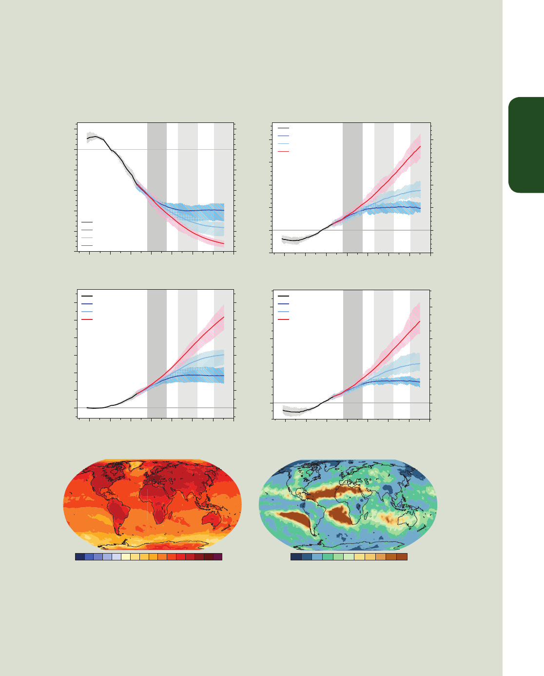
TS
Technical Summary
111
a different rate than the mean warming however, with several studies showing that projected European high-
percentile summer temperatures will warm faster than mean temperatures. Future changes associated with the
warming of temperature extremes in the long-term are virtually certain and scale with the strength of emissions
scenario, that is, greater anthropogenic emissions correspond to greater warming of extremes (TFE.9, Figure 1). For
high-emissions scenarios, it is likely that, in most land regions, a current 1-in-20-year maximum temperature event
TFE.9, Figure 1 | Global projections of the occurrence of (a) cold days (TX10p)- percentage of days annually with daily maximum surface air temperature (Tmax) below
the 10th percentile of Tmax for 1961 to 1990, (b) wettest consecutive 5 days (RX5day) —percentage change relative to 1986–2005 in annual maximum consecutive
5-day precipitation totals, (c) warm days (TX90p)—percentage of days annually with daily maximum surface air temperature (Tmax) exceeding the 90th percentile
of Tmax for 1961 to 1990 and (d) very wet day precipitation (R95p)—percentage change relative to 1986–2005 of annual precipitation from days >95th percentile.
Results are shown from CMIP5 for the RCP2.6, RCP4.5 and RCP8.5 scenarios. Solid lines indicate the ensemble median and shading indicates the interquartile spread
between individual projections (25th and 75th percentiles). Maps show (e) the change from 1986–2005 to 2081–2100 in 20-year return values (RV) of daily maximum
temperatures, TXx, and (f) the 2081–2100 return period (RP) for rare daily precipitation values, RX1day, that have a 20-year return period during 1986–2005. Both
maps are based on the CMIP5 RCP8.5 scenario. The number of models used to calculate the multi-model mean is indicated in each panel. See Box 2.4, Table 1 for index
definitions. {Figures 11.17, 12.14, 12.26, 12.27}
TFE.9 (continued)
1960 1980 2000 2020 2040 2060 2080 2100
0
2
4
6
8
10
12
Year
Exceedance rate (%)
0
2
4
6
8
10
12
Cold days (TX10p)
historical
RCP2.6
RCP4.5
RCP8.5
historical
RCP2.6
RCP4.5
RCP8.5
historical
RCP2.6
RCP4.5
RCP8.5
historical
RCP2.6
RCP4.5
RCP8.5
1960 1980 2000 2020 2040 2060 2080 2100
−5
0
5
10
15
20
Year
Relative change (%)
−5
0
5
10
15
20
Wettest consecutive five days (RX5day)
1960 1980 2000 2020 2040 2060 2080 2100
10
20
30
40
50
60
70
Year
Exceedance rate (%)
10
20
30
40
50
60
70
Warm days (TX90p)
1960 1980 2000 2020 2040 2060 2080 2100
0
20
40
60
Year
Relative change (%)
0
20
40
60
Precipitation from very wet days (R95p)
(a)(b)
(d)(c)
(e)
(f)
Future change in 20yr RV of warmest daily Tmax (TXx)
Future RP for present day 20yr RV of wettest day (RX1day)
(°C)
Years
-0.5-1-1.5-2 1.510.50 864214161820121054321197
29
18
18
18
18
29
(continued on next page)

TS
Technical Summary
112
will at least double in frequency but in many regions will become an annual or a 1-in-2-year event by the end of
the 21st century. The magnitude of both high and low temperature extremes is expected to increase at least at the
same rate as the mean, but with 20-year return values for low temperature events projected to increase at a rate
greater than winter mean temperatures in most regions. {10.6.1, 11.3.2, 12.4.3}
Precipitation Extremes
It is likely that the number of heavy precipitation events over land has increased in more regions than it has
decreased in since the mid-20th century, and there is medium confidence that anthropogenic forcing has contrib-
uted to this increase. {2.6.2, 10.6.1}
There has been substantial progress between CMIP3 and CMIP5 in the ability of models to simulate more realistic
precipitation extremes. However, evidence suggests that the majority of models underestimate the sensitivity of
extreme precipitation to temperature variability or trends especially in the tropics, which implies that models may
underestimate the projected increase in extreme precipitation in the future. While progress has been made in
understanding the processes that drive extreme precipitation, challenges remain in quantifying cloud and convec-
tive effects in models for example. The complexity of land surface and atmospheric processes limits confidence in
regional projections of precipitation change, especially over land, although there is a component of a ‘wet-get-
wetter’ and ‘dry-get-drier’ response over oceans at the large scale. Even so, there is high confidence that, as the
climate warms, extreme precipitation rates (e.g., on daily time scales) will increase faster than the time average.
Changes in local extremes on daily and sub-daily time scales are expected to increase by roughly 5 to 10% per °C of
warming (medium confidence). {7.6, 9.5.4}
For the near and long term, CMIP5 projections confirm a clear tendency for increases in heavy precipitation events
in the global mean seen in the AR4, but there are substantial variations across regions (TFE.9, Figure 1). Over most
of the mid-latitude land masses and over wet tropical regions, extreme precipitation will very likely be more intense
and more frequent in a warmer world. {11.3.2, 12.4.5}
Floods and Droughts
There continues to be a lack of evidence and thus low confidence regarding the sign of trend in the magnitude
and/or frequency of floods on a global scale over the instrumental record. There is high confidence that past floods
larger than those recorded since 1900 have occurred during the past five centuries in northern and central Europe,
western Mediterranean region, and eastern Asia. There is medium confidence that modern large floods are com-
parable to or surpass historical floods in magnitude and/or frequency in the Near East, India and central North
America. {2.6.2, 5.5.5}
Compelling arguments both for and against significant increases in the land area affected by drought and/or dry-
ness since the mid-20th century have resulted in a low confidence assessment of observed and attributable large-
scale trends. This is due primarily to a lack and quality of direct observations, dependencies of inferred trends on the
index choice, geographical inconsistencies in the trends and difficulties in distinguishing decadal scale variability
from long term trends. On millennial time scales, there is high confidence that proxy information provides evidence
of droughts of greater magnitude and longer duration than observed during the 20th century in many regions.
There is medium confidence that more megadroughts occurred in monsoon Asia and wetter conditions prevailed
in arid Central Asia and the South American monsoon region during the Little Ice Age (1450 to 1850) compared to
the Medieval Climate Anomaly (950 to 1250). {2.6.2, 5.5.4, 5.5.5, 10.6.1}
Under the Representative Concentration Pathway RCP8.5, projections by the end of the century indicate an
increased risk of drought is likely (medium confidence) in presently dry regions linked to regional to global-scale
projected decreases in soil moisture. Soil moisture drying is most prominent in the Mediterranean, Southwest USA,
and southern Africa, consistent with projected changes in the Hadley Circulation and increased surface tempera-
tures, and surface drying in these regions is likely (high confidence) by the end of the century under RCP8.5. {12.4.5}
Extreme Sea Level
It is likely that the magnitude of extreme high sea level events has increased since 1970 and that most of this rise can
be explained by increases in mean sea level. When mean sea level changes is taken into account, changes in extreme
high sea levels are reduced to less than 5 mm y
r–1
at 94% of tide gauges. In the future it is very likely that there will
be a significant increase in the occurrence of sea level extremes and similarly to past observations, this increase will
primarily be the result of an increase in mean sea level. {3.7.5, 13.7.2}
TFE.9 (continued)
(continued on next page)

TS
Technical Summary
113
Tropical and Extratropical Cyclones
There is low confidence in long-term (centennial) changes in tropical cyclone activity, after accounting for past
changes in observing capabilities. However over the satellite era, increases in the frequency and intensity of the
strongest storms in the North Atlantic are robust (very high confidence). However, the cause of this increase is
debated and there is low confidence in attribution of changes in tropical cyclone activity to human influence owing
to insufficient observational evidence, lack of physical understanding of the links between anthropogenic drivers of
climate and tropical cyclone activity and the low level of agreement between studies as to the relative importance
of internal variability, and anthropogenic and natural forcings. {2.6.3, 10.6.1, 14.6.1}
Some high-resolution atmospheric models have realistically simulated tracks and counts of tropical cyclones and
models generally are able to capture the general characteristics of storm tracks and extratropical cyclones with evi-
dence of improvement since the AR4. Storm track biases in the North Atlantic have improved slightly, but models
still produce a storm track that is too zonal and underestimate cyclone intensity. {9.4.1, 9.5.4}
While projections indicate that it is likely that the global frequency of tropical cyclones will either decrease or
remain essentially unchanged, concurrent with a likely increase in both global mean tropical cyclone maximum
wind speed and rainfall rates, there is lower confidence in region-specific projections of frequency and intensity.
However, due to improvements in model resolution and downscaling techniques, it is more likely than not that the
frequency of the most intense storms will increase substantially in some basins under projected 21st century warm-
ing (see Figure TS.26). {11.3.2, 14.6.1}
Research subsequent to the AR4 and SREX continues to support a likely poleward shift of storm tracks since the
1950s. However over the last century there is low confidence of a clear trend in storminess due to inconsistencies
between studies or lack of long-term data in some parts of the world (particularly in the Southern Hemisphere (SH)).
{2.6.4, 2.7.6}
Despite systematic biases in simulating storm tracks, most models and studies are in agreement that the global
number of extratropical cyclones is unlikely to decrease by more than a few per cent. A small poleward shift is
likely in the SH storm track. It is more likely than not (medium confidence) for a projected poleward shift in the
North Pacific storm track but it is unlikely that the response of the North Atlantic storm track is a simple poleward
shift. There is low confidence in the magnitude of regional storm track changes, and the impact of such changes
on regional surface climate. {14.6.2}
TFE.9 (continued)

TS
Technical Summary
114
TS.6 Key Uncertainties
This final section of the Technical Summary provides readers with a
short overview of key uncertainties in the understanding of the climate
system and the ability to project changes in response to anthropogenic
influences. The overview is not comprehensive and does not describe in
detail the basis for these findings. These are found in the main body of
this Technical Summary and in the underlying chapters to which each
bullet points in the curly brackets.
TS.6.1 Key Uncertainties in Observation of Changes in
the Climate System
• There is only medium to low confidence in the rate of change of
tropospheric warming and its vertical structure. Estimates of tro-
pospheric warming rates encompass surface temperature warm-
ing rate estimates. There is low confidence in the rate and vertical
structure of the stratospheric cooling. {2.4.4}
• Confidence in global precipitation change over land is low prior
to 1951 and medium afterwards because of data incompleteness.
{2.5.1}
• Substantial ambiguity and therefore low confidence remains in the
observations of global-scale cloud variability and trends. {2.5.6}
• There is low confidence in an observed global-scale trend in
drought or dryness (lack of rainfall), due to lack of direct observa-
tions, methodological uncertainties and choice and geographical
inconsistencies in the trends. {2.6.2}
• There is low confidence that any reported long-term (centen-
nial) changes in tropical cyclone characteristics are robust, after
accounting for past changes in observing capabilities. {2.6.3}
• Robust conclusions on long-term changes in large-scale atmos-
pheric circulation are presently not possible because of large vari-
ability on interannual to decadal time scales and remaining differ-
ences between data sets. {2.7}
• Different global estimates of sub-surface ocean temperatures have
variations at different times and for different periods, suggesting
that sub-decadal variability in the temperature and upper heat
content (0 to to 700 m) is still poorly characterized in the historical
record. {3.2}
• Below ocean depths of 700 m the sampling in space and time is
too sparse to produce annual global ocean temperature and heat
content estimates prior to 2005. {3.2.4}
• Observational coverage of the ocean deeper than 2000 m is still
limited and hampers more robust estimates of changes in global
ocean heat content and carbon content. This also limits the quan-
tification of the contribution of deep ocean warming to sea level
rise. {3.2, 3.7, 3.8; Box 3.1}
• The number of continuous observational time series measuring the
strength of climate relevant ocean circulation features (e.g., the
meridional overturning circulation) is limited and the existing time
series are still too short to assess decadal and longer trends. {3.6}.
• In Antarctica, available data are inadequate to assess the status
of change of many characteristics of sea ice (e.g., thickness and
volume). {4.2.3}
• On a global scale the mass loss from melting at calving fronts and
iceberg calving are not yet comprehensively assessed. The largest
uncertainty in estimated mass loss from glaciers comes from the
Antarctic, and the observational record of ice–ocean interactions
around both ice sheets remains poor. {4.3.3, 4.4}
TS.6.2 Key Uncertainties in Drivers of Climate Change
• Uncertainties in aerosol–cloud interactions and the associated
radiative forcing remain large. As a result, uncertainties in aerosol
forcing remain the dominant contributor to the overall uncertainty
in net anthropogenic forcing, despite a better understanding of
some of the relevant atmospheric processes and the availability of
global satellite monitoring. {2.2, 7.3–7.5, 8.5}
• The cloud feedback is likely positive but its quantification remains
difficult. {7.2}
• Paleoclimate reconstructions and Earth System Models indicate
that there is a positive feedback between climate and the carbon
cycle, but confidence remains low in the strength of this feedback,
particularly for the land. {6.4}
TS.6.3 Key Uncertainties in Understanding the Climate
System and Its Recent Changes
• The simulation of clouds in AOGCMs has shown modest improve-
ment since AR4; however, it remains challenging. {7.2, 9.2.1, 9.4.1,
9.7.2}
• Observational uncertainties for climate variables other than tem-
perature, uncertainties in forcings such as aerosols, and limits in
process understanding continue to hamper attribution of changes
in many aspects of the climate system. {10.1, 10.3, 10.7}
• Changes in the water cycle remain less reliably modelled in both
their changes and their internal variability, limiting confidence in
attribution assessments. Observational uncertainties and the large
effect of internal variability on observed precipitation also pre-
cludes a more confident assessment of the causes of precipitation
changes. {2.5.1, 2.5.4, 10.3.2}
• Modelling uncertainties related to model resolution and incorpo-
ration of relevant processes become more important at regional
scales, and the effects of internal variability become more signifi-
cant. Therefore, challenges persist in attributing observed change
to external forcing at regional scales. {2.4.1, 10.3.1}

TS
Technical Summary
115
• The ability to simulate changes in frequency and intensity of
extreme events is limited by the ability of models to reliably simu-
late mean changes in key features. {10.6.1}
• In some aspects of the climate system, including changes in
drought, changes in tropical cyclone activity, Antarctic warming,
Antarctic sea ice extent, and Antarctic mass balance, confidence
in attribution to human influence remains low due to model-
ling uncertainties and low agreement between scientific studies.
{10.3.1, 10.5.2, 10.6.1}
TS.6.4 Key Uncertainties in Projections of Global and
Regional Climate Change
• Based on model results there is limited confidence in the predict-
ability of yearly to decadal averages of temperature both for the
global average and for some geographical regions. Multi-model
results for precipitation indicate a generally low predictability.
Short-term climate projection is also limited by the uncertainty in
projections of natural forcing. {11.1, 11.2, 11.3.1, 11.3.6; Box 11.1}
• There is medium confidence in near-term projections of a north-
ward shift of NH storm track and westerlies. {11.3.2}
• There is generally low confidence in basin-scale projections of sig-
nificant trends in tropical cyclone frequency and intensity in the
21st century. {11.3.2, 14.6.1}
• Projected changes in soil moisture and surface run off are not
robust in many regions. {11.3.2, 12.4.5}
• Several components or phenomena in the climate system could
potentially exhibit abrupt or nonlinear changes, but for many phe-
nomena there is low confidence and little consensus on the likeli-
hood of such events over the 21st century. {12.5.5}
• There is low confidence on magnitude of carbon losses through
CO
2
or CH
4
emissions to the atmosphere from thawing perma-
frost. There is low confidence in projected future CH
4
emissions
from natural sources due to changes in wetlands and gas hydrate
release from the sea floor. {6.4.3, 6.4.7}
• There is medium confidence in the projected contributions to sea
level rise by models of ice sheet dynamics for the 21st century, and
low confidence in their projections beyond 2100. {13.3.3}
• There is low confidence in semi-empirical model projections of
global mean sea level rise, and no consensus in the scientific com-
munity about their reliability. {13.5.2, 13.5.3}
• There is low confidence in projections of many aspects of climate
phenomena that influence regional climate change, including
changes in amplitude and spatial pattern of modes of climate vari-
ability. {9.5.3, 14.2–14.7}
