
465
6
This chapter should be cited as:
Ciais, P., C. Sabine, G. Bala, L. Bopp, V. Brovkin, J. Canadell, A. Chhabra, R. DeFries, J. Galloway, M. Heimann, C.
Jones, C. Le Quéré, R.B. Myneni, S. Piao and P. Thornton, 2013: Carbon and Other Biogeochemical Cycles. In: Cli-
mate Change 2013: The Physical Science Basis. Contribution of Working Group I to the Fifth Assessment Report
of the Intergovernmental Panel on Climate Change [Stocker, T.F., D. Qin, G.-K. Plattner, M. Tignor, S.K. Allen, J.
Boschung, A. Nauels, Y. Xia, V. Bex and P.M. Midgley (eds.)]. Cambridge University Press, Cambridge, United
Kingdom and New York, NY, USA.
Coordinating Lead Authors:
Philippe Ciais (France), Christopher Sabine (USA)
Lead Authors:
Govindasamy Bala (India), Laurent Bopp (France), Victor Brovkin (Germany/Russian Federation),
Josep Canadell (Australia), Abha Chhabra (India), Ruth DeFries (USA), James Galloway (USA),
Martin Heimann (Germany), Christopher Jones (UK), Corinne Le Quéré (UK), Ranga B. Myneni
(USA), Shilong Piao (China), Peter Thornton (USA)
Contributing Authors:
Anders Ahlström (Sweden), Alessandro Anav (UK/Italy), Oliver Andrews (UK), David Archer
(USA), Vivek Arora (Canada), Gordon Bonan (USA), Alberto Vieira Borges (Belgium/Portugal),
Philippe Bousquet (France), Lex Bouwman (Netherlands), Lori M. Bruhwiler (USA), Kenneth
Caldeira (USA), Long Cao (China), Jérôme Chappellaz (France), Frédéric Chevallier (France),
Cory Cleveland (USA), Peter Cox (UK), Frank J. Dentener (EU/Netherlands), Scott C. Doney
(USA), Jan Willem Erisman (Netherlands), Eugenie S. Euskirchen (USA), Pierre Friedlingstein
(UK/Belgium), Nicolas Gruber (Switzerland), Kevin Gurney (USA), Elisabeth A. Holland (Fiji/
USA), Brett Hopwood (USA), Richard A. Houghton (USA), Joanna I. House (UK), Sander
Houweling (Netherlands), Stephen Hunter (UK), George Hurtt (USA), Andrew D. Jacobson
(USA), Atul Jain (USA), Fortunat Joos (Switzerland), Johann Jungclaus (Germany), Jed O. Kaplan
(Switzerland/Belgium/USA), Etsushi Kato (Japan), Ralph Keeling (USA), Samar Khatiwala
(USA), Stefanie Kirschke (France/Germany), Kees Klein Goldewijk (Netherlands), Silvia Kloster
(Germany), Charles Koven (USA), Carolien Kroeze (Netherlands), Jean-François Lamarque
(USA/Belgium), Keith Lassey (New Zealand), Rachel M. Law (Australia), Andrew Lenton
(Australia), Mark R. Lomas (UK), Yiqi Luo (USA), Takashi Maki (Japan), Gregg Marland (USA),
H. Damon Matthews (Canada), Emilio Mayorga (USA), Joe R. Melton (Canada), Nicolas Metzl
(France), Guy Munhoven (Belgium/Luxembourg), Yosuke Niwa (Japan), Richard J. Norby (USA),
Fiona O’Connor (UK/Ireland), James Orr (France), Geun-Ha Park (USA), Prabir Patra (Japan/
India), Anna Peregon (France/Russian Federation), Wouter Peters (Netherlands), Philippe Peylin
(France), Stephen Piper (USA), Julia Pongratz (Germany), Ben Poulter (France/USA), Peter A.
Raymond (USA), Peter Rayner (Australia), Andy Ridgwell (UK), Bruno Ringeval (Netherlands/
France), Christian Rödenbeck (Germany), Marielle Saunois (France), Andreas Schmittner
(USA/Germany), Edward Schuur (USA), Stephen Sitch (UK), Renato Spahni (Switzerland),
Benjamin Stocker (Switzerland), Taro Takahashi (USA), Rona L. Thompson (Norway/New
Zealand), Jerry Tjiputra (Norway/Indonesia), Guido van der Werf (Netherlands), Detlef van
Vuuren (Netherlands), Apostolos Voulgarakis (UK/Greece), Rita Wania (Austria), Sönke Zaehle
(Germany), Ning Zeng (USA)
Review Editors:
Christoph Heinze (Norway), Pieter Tans (USA), Timo Vesala (Finland)
Carbon and Other
Biogeochemical Cycles

466
6
Table of Contents
Executive Summary ..................................................................... 467
6.1 Introduction ...................................................................... 470
6.1.1 Global Carbon Cycle Overview .................................. 470
Box 6.1: Multiple Residence Times for an Excess of Carbon
Dioxide Emitted in the Atmosphere ........................................ 472
6.1.2 Industrial Era ............................................................. 474
6.1.3 Connections Between Carbon and the Nitrogen
and Oxygen Cycles .................................................... 475
Box 6.2: Nitrogen Cycle and Climate-Carbon
Cycle Feedbacks ......................................................................... 477
6.2 Variations in Carbon and Other Biogeochemical
Cycles Before the Fossil Fuel Era ................................ 480
6.2.1 Glacial–Interglacial Greenhouse Gas Changes .......... 480
6.2.2 Greenhouse Gas Changes over the Holocene ........... 483
6.2.3 Greenhouse Gas Changes over the
Last Millennium ........................................................ 485
6.3 Evolution of Biogeochemical Cycles Since the
Industrial Revolution ..................................................... 486
6.3.1 Carbon Dioxide Emissions and Their Fate
Since 1750 ................................................................ 486
6.3.2 Global Carbon Dioxide Budget .................................. 488
Box 6.3: The Carbon Dioxide Fertilisation Effect ................... 502
6.3.3 Global Methane Budget ............................................ 508
6.3.4 Global Nitrogen Budgets and Global Nitrous
Oxide Budget in the 1990s ........................................ 510
6.4. Projections of Future Carbon and Other
Biogeochemical Cycles .................................................. 514
6.4.1 Introduction .............................................................. 514
6.4.2 Carbon Cycle Feedbacks in Climate Modelling
Intercomparison Project Phase 5 Models .................. 514
Box 6.4: Climate–Carbon Cycle Models and
Experimental Design ................................................................. 516
6.4.3 Implications of the Future Projections for the
Carbon Cycle and Compatible Emissions .................. 523
6.4.4 Future Ocean Acidification ........................................ 528
6.4.5 Future Ocean Oxygen Depletion ............................... 532
6.4.6 Future Trends in the Nitrogen Cycle and Impact
on Carbon Fluxes ...................................................... 535
6.4.7 Future Changes in Methane Emissions ..................... 539
6.4.8 Other Drivers of Future Carbon Cycle Changes ......... 542
6.4.9 The Long-term Carbon Cycle and Commitments ....... 543
6.5 Potential Effects of Carbon Dioxide Removal
Methods and Solar Radiation Management
on the Carbon Cycle ....................................................... 546
6.5.1 Introduction to Carbon Dioxide
Removal Methods ..................................................... 546
6.5.2 Carbon Cycle Processes Involved in Carbon
Dioxide Removal Methods ........................................ 547
6.5.3 Impacts of Carbon Dioxide Removal Methods on
Carbon Cycle and Climate ......................................... 550
6.5.4 Impacts of Solar Radiation Management on the
Carbon Cycle ............................................................. 551
6.5.5 Synthesis ................................................................... 552
References .................................................................................. 553
Frequently Asked Questions
FAQ 6.1 Could Rapid Release of Methane and Carbon
Dioxide from Thawing Permafrost or Ocean
Warming Substantially Increase Warming? ........ 530
FAQ 6.2 What Happens to Carbon Dioxide After It Is
Emitted into the Atmosphere? ............................. 544
Supplementary Material
Supplementary Material is available in online versions of the report.

467
Carbon and Other Biogeochemical Cycles Chapter 6
6
1
In this Report, the following summary terms are used to describe the available evidence: limited, medium, or robust; and for the degree of agreement: low, medium, or
high. A level of confidence is expressed using five qualifiers: very low, low, medium, high, and very high, and typeset in italics, e.g., medium confidence. For a given evi-
dence and agreement statement, different confidence levels can be assigned, but increasing levels of evidence and degrees of agreement are correlated with increasing
confidence (see Section 1.4 and Box TS.1 for more details).
2
In this Report, the following terms have been used to indicate the assessed likelihood of an outcome or a result: Virtually certain 99–100% probability, Very likely
90–100%, Likely 66–100%, About as likely as not 33–66%, Unlikely 0–33%, Very unlikely 0–10%, Exceptionally unlikely 0–1%. Additional terms (Extremely likely:
95–100%, More likely than not >50–100%, and Extremely unlikely 0–5%) may also be used when appropriate. Assessed likelihood is typeset in italics, e.g., very likely
(see Section 1.4 and Box TS.1 for more details).
Executive Summary
This chapter addresses the biogeochemical cycles of carbon dioxide
(CO
2
), methane (CH
4
) and nitrous oxide (N
2
O). The three greenhouse
gases (GHGs) have increased in the atmosphere since pre-industrial
times, and this increase is the main driving cause of climate change
(Chapter 10). CO
2
, CH
4
and N
2
O altogether amount to 80% of the total
radiative forcing from well-mixed GHGs (Chapter 8). The increase of
CO
2
, CH
4
and N
2
O is caused by anthropogenic emissions from the use
of fossil fuel as a source of energy and from land use and land use
changes, in particular agriculture. The observed change in the atmos-
pheric concentration of CO
2
, CH
4
and N
2
O results from the dynamic
balance between anthropogenic emissions, and the perturbation of
natural processes that leads to a partial removal of these gases from
the atmosphere. Natural processes are linked to physical conditions,
chemical reactions and biological transformations and they respond
themselves to perturbed atmospheric composition and climate change.
Therefore, the physical climate system and the biogeochemical cycles
of CO
2
, CH
4
and N
2
O are coupled. This chapter addresses the present
human-caused perturbation of the biogeochemical cycles of CO
2
, CH
4
and N
2
O, their variations in the past coupled to climate variations and
their projected evolution during this century under future scenarios.
The Human-Caused Perturbation in the Industrial Era
CO
2
increased by 40% from 278 ppm about 1750 to 390.5 ppm
in 2011. During the same time interval, CH
4
increased by 150%
from 722 ppb to 1803 ppb, and N
2
O by 20% from 271 ppb to
324.2 ppb in 2011. It is unequivocal that the current concentrations
of atmospheric CO
2
, CH
4
and N
2
O exceed any level measured for at
least the past 800,000 years, the period covered by ice cores. Further-
more, the average rate of increase of these three gases observed over
the past century exceeds any observed rate of change over the previ-
ous 20,000 years. {2.2, 5.2, 6.1, 6.2}
Anthropogenic CO
2
emissions to the atmosphere were 555 ± 85
PgC (1 PgC = 10
15
gC) between 1750 and 2011. Of this amount,
fossil fuel combustion and cement production contributed 375 ± 30
PgC and land use change (including deforestation, afforestation and
reforestation) contributed 180 ± 80 PgC. {6.3.1, Table 6.1}
With a very high level of confidence
1
, the increase in CO
2
emis-
sions from fossil fuel burning and those arising from land
use change are the dominant cause of the observed increase
in atmospheric CO
2
concentration. About half of the emissions
remained in the atmosphere (240 ± 10 PgC) since 1750. The rest
was removed from the atmosphere by sinks and stored in the natural
carbon cycle reservoirs. The ocean reservoir stored 155 ± 30 PgC. Veg-
etation biomass and soils not affected by land use change stored 160
± 90 PgC. {6.1, 6.3, 6.3.2.3, Table 6.1, Figure 6.8}
Carbon emissions from fossil fuel combustion and cement pro-
duction increased faster during the 2000–2011 period than
during the 1990–1999 period. These emissions were 9.5 ± 0.8 PgC
yr
–1
in 2011, 54% above their 1990 level. Anthropogenic net CO
2
emis-
sions from land use change were 0.9 ± 0.8 PgC yr
–1
throughout the
past decade, and represent about 10% of the total anthropogenic CO
2
emissions. It is more likely than not
2
that net CO
2
emissions from land
use change decreased during 2000–2011 compared to 1990–1999.
{6.3, Table 6.1, Table 6.2, Figure 6.8}
Atmospheric CO
2
concentration increased at an average rate
of 2.0 ± 0.1 ppm yr
–1
during 2002–2011. This decadal rate of
increase is higher than during any previous decade since direct
atmospheric concentration measurements began in 1958. Glob-
ally, the size of the combined natural land and ocean sinks of CO
2
approximately followed the atmospheric rate of increase, removing
55% of the total anthropogenic emissions every year on average
during 1958–2011. {6.3, Table 6.1}
After almost one decade of stable CH
4
concentrations since the
late 1990s, atmospheric measurements have shown renewed
CH
4
concentrations growth since 2007. The drivers of this renewed
growth are still debated. The methane budget for the decade of 2000–
2009 (bottom-up estimates) is 177 to 284 Tg(CH
4
) yr
–1
for natural
wetlands emissions, 187 to 224 Tg(CH
4
) yr
–1
for agriculture and waste
(rice, animals and waste), 85 to 105 Tg(CH
4
) yr
–1
for fossil fuel related
emissions, 61 to 200 Tg(CH
4
) yr
–1
for other natural emissions including,
among other fluxes, geological, termites and fresh water emissions,
and 32 to 39 Tg(CH
4
) yr
–1
for biomass and biofuel burning (the range
indicates the expanse of literature values). Anthropogenic emissions
account for 50 to 65% of total emissions. By including natural geo-
logical CH
4
emissions that were not accounted for in previous budg-
ets, the fossil component of the total CH
4
emissions (i.e., anthropo-
genic emissions related to leaks in the fossil fuel industry and natural
geological leaks) is now estimated to amount to about 30% of the
total CH
4
emissions (medium confidence). Climate driven fluctuations
of CH
4
emissions from natural wetlands are the main drivers of the
global interannual variability of CH
4
emissions (high confidence), with
a smaller contribution from the variability in emissions from biomass
burning during high fire years. {6.3.3, Figure 6.2, Table 6.8}
The concentration of N
2
O increased at a rate of 0.73 ± 0.03 ppb
yr
–1
over the last three decades. Emissions of N
2
O to the atmos-
phere are mostly caused by nitrification and de-nitrification reactions

468
Chapter 6 Carbon and Other Biogeochemical Cycles
6
of reactive nitrogen in soils and in the ocean. Anthropogenic N
2
O emis-
sions increasedsteadily over the last two decades and were 6.9 (2.7
to 11.1) TgN (N
2
O) yr
–1
in 2006. Anthropogenic N
2
O emissions are 1.7
to 4.8 TgN (N
2
O) yr
–1
from the application of nitrogenous fertilisers in
agriculture, 0.2 to 1.8 TgN (N
2
O) yr
–1
from fossil fuel use and industrial
processes, 0.2 to 1.0 TgN (N
2
O) yr
–1
from biomass burning (including
biofuels) and 0.4 to 1.3 TgN (N
2
O) yr
–1
from land emissions due to
atmospheric nitrogen deposition (the range indicates expand of liter-
ature values). Natural N
2
O emissions derived from soils, oceans and a
small atmospheric source are together 5.4 to 19.6 TgN (N
2
O) yr
–1
. {6.3,
6.3.4, Figure 6.4c, Figure 6.19, Table 6.9}
The human-caused creation of reactive nitrogen in 2010 was at
least two times larger than the rate of natural terrestrial cre-
ation. The human-caused creation of reactive nitrogen is dominated
by the production of ammonia for fertiliser and industry, with impor-
tant contributions from legume cultivation and combustion of fossil
fuels. Once formed, reactive nitrogen can be transferred to waters
and the atmosphere. In addition to N
2
O, two important nitrogen com-
pounds emitted to the atmosphere are NH
3
and NO
x
both of which
influence tropospheric O
3
and aerosols through atmospheric chemis-
try. All of these effects contribute to radiative forcing. It is also likely
that reactive nitrogen deposition over land currently increases natural
CO
2
sinks, in particular forests, but the magnitude of this effect varies
between regions. {6.1.3, 6.3, 6.3.2.6.5, 6.3.4, 6.4.6, Figures 6.4a and
6.4b, Table 6.9, Chapter 7}
Before the Human-Caused Perturbation
During the last 7000 years prior to 1750, atmospheric CO
2
from
ice cores shows only very slow changes (increase) from 260
ppm to 280 ppm, in contrast to the human-caused increase of
CO
2
since pre-industrial times. The contribution of CO
2
emis-
sions from early anthropogenic land use is unlikely sufficient
to explain the CO
2
increase prior to 1750. Atmospheric CH
4
from
ice cores increased by about 100 ppb between 5000 years ago and
around 1750. About as likely as not, this increase can be attributed to
early human activities involving livestock, human-caused fires and rice
cultivation. {6.2, Figures 6.6 and 6.7}
Further back in time, during the past 800,000 years prior to
1750, atmospheric CO
2
varied from 180 ppm during glacial
(cold) up to 300 ppm during interglacial (warm) periods. This
is well established from multiple ice core measurements. Variations in
atmospheric CO
2
from glacial to interglacial periods were caused by
decreased ocean carbon storage (500 to 1200 PgC), partly compensat-
ed by increased land carbon storage (300 to 1000 PgC). {6.2.1, Figure
6.5}
Future Projections
With very high confidence, ocean carbon uptake of anthropo-
genic CO
2
emissions will continue under all four Representative
Concentration Pathways (RCPs) through to 2100, with higher
uptake corresponding to higher concentration pathways. The
future evolution of the land carbon uptake is much more uncertain,
with a majority of models projecting a continued net carbon uptake
under all RCPs, but with some models simulating a net loss of carbon
by the land due to the combined effect of climate change and land use
change. In view of the large spread of model results and incomplete
process representation, there is low confidence on the magnitude of
modelled future land carbon changes. {6.4.3, Figure 6.24}
There is high confidence that climate change will partially offset
increases in global land and ocean carbon sinks caused by rising
atmospheric CO
2
. Yet, there are regional differences among Climate
Modelling Intercomparison Project Phase 5 (CMIP5) Earth System
Models, in the response of ocean and land CO
2
fluxes to climate. There
is a high agreement between models that tropical ecosystems will store
less carbon in a warmer climate. There is medium agreement between
models that at high latitudes warming will increase land carbon stor-
age, although none of the models account for decomposition of carbon
in permafrost, which may offset increased land carbon storage. There
is high agreement between CMIP5 Earth System models that ocean
warming and circulation changes will reduce the rate of carbon uptake
in the Southern Ocean and North Atlantic, but that carbon uptake will
nevertheless persist in those regions. {6.4.2, Figures 6.21 and 6.22}
It is very likely, based on new experimental results {6.4.6.3} and
modelling, that nutrient shortage will limit the effect of rising
atmospheric CO
2
on future land carbon sinks, for the four RCP
scenarios. There is high confidence that low nitrogen availability will
limit carbon storage on land, even when considering anthropogenic
nitrogen deposition. The role of phosphorus limitation is more uncer-
tain. Models that combine nitrogen limitations with rising CO
2
and
changes in temperature and precipitation thus produce a systematical-
ly larger increase in projected future atmospheric CO
2
, for a given fossil
fuel emissions trajectory. {6.4.6, 6.4.6.3, 6.4.8.2, Figure 6.35}
Taking climate and carbon cycle feedbacks into account, we
can quantify the fossil fuel emissions compatible with the
RCPs. Between 2012 and 2100, the RCP2.6, RCP4.5, RCP6.0, and
RCP8.5 scenarios imply cumulative compatible fossil fuel emis-
sions of 270 (140 to 410) PgC, 780(595 to 1005) PgC, 1060 (840
to 1250) PgC and 1685(1415 to 1910) PgC respectively (values
quoted to nearest 5 PgC, range derived from CMIP5 model results).
For RCP2.6, an average 50% (range 14 to 96%) emission reduction is
required by 2050 relative to 1990 levels. By the end of the 21st century,
about half of the models infer emissions slightly above zero, while the
other half infer a net removal of CO
2
from the atmosphere. {6.4.3, Table
6.12, Figure 6.25}
There is high confidence that reductions in permafrost extent
due to warming will cause thawing of some currently frozen
carbon. However, there is low confidence on the magnitude of
carbon losses through CO
2
and CH
4
emissions to the atmosphere,
with a range from 50 to 250 PgC between 2000 and 2100 under the
RCP8.5 scenario. The CMIP5 Earth System Models did not include
frozen carbon feedbacks. {6.4.3.4, Chapter 12}
There is medium confidence that emissions of CH
4
from wet-
lands are likely to increase under elevated CO
2
and a warmer
climate. But there is low confidence in quantitative projections of
these changes. The likelihood of the future release of CH
4
from marine

469
Carbon and Other Biogeochemical Cycles Chapter 6
6
gas hydrates in response to seafloor warming is poorly understood. In
the event of a significant release of CH
4
from hydrates in the sea floor
by the end of the 21st century, it is likely that subsequent emissions to
the atmosphere would be in the form of CO
2
, due to CH
4
oxidation in
the water column. {6.4.7, Figure 6.37}
It is likely that N
2
O emissions from soils will increase due to the
increased demand for feed/food and the reliance of agriculture
on nitrogen fertilisers. Climate warming will likely amplify agricul-
tural and natural terrestrial N
2
O sources, but there is low confidence in
quantitative projections of these changes. {6.4.6, Figure 6.32}
It is virtually certain that the increased storage of carbon by the
ocean will increase acidification in the future, continuing the
observed trends of the past decades. Ocean acidification in the
surface ocean will follow atmospheric CO
2
while it will also increase
in the deep ocean as CO
2
continues to penetrate the abyss. The CMIP5
models consistently project worldwide increased ocean acidification to
2100 under all RCPs. The corresponding decrease in surface ocean pH
by the end of the 21st century is 0.065 (0.06 to 0.07) for RCP2.6, 0.145
(0.14 to 0.15) for RCP4.5, 0.203 (0.20 to 0.21) for RCP6.0, and 0.31
(0.30 to 0.32) for RCP8.5 (range from CMIP5 models spread). Surface
waters become seasonally corrosive to aragonite in parts of the Arctic
and in some coastal upwelling systems within a decade, and in parts of
the Southern Ocean within 1 to 3 decades in most scenarios. Aragonite
undersaturation becomes widespread in these regions atatmospheric
CO
2
levels of 500 to 600 ppm. {6.4.4, Figures 6.28 and 6.29}
It is very likely that the dissolved oxygen content of the ocean
will decrease by a few percent during the 21st century. CMIP5
models suggest that this decrease in dissolved oxygen will predomi-
nantly occur in the subsurface mid-latitude oceans, caused by enhanced
stratification, reduced ventilation and warming. However, there is no
consensus on the future development of the volume of hypoxic and
suboxic waters in the open-ocean because of large uncertainties in
potential biogeochemical effects and in the evolution of tropical ocean
dynamics. {6.4.5, Figure 6.30}
Irreversible Long-Term Impacts of Human-Caused Emissions
Withvery high confidence, the physical, biogeochemical carbon
cycle in the ocean and on land will continue to respond to cli-
mate change and rising atmospheric CO
2
concentrations created
during the 21st century. Ocean acidification will very likely continue
in the future as long as the oceans take up atmospheric CO
2
. Com-
mitted land ecosystem carbon cycle changes will manifest themselves
further beyond the end of the 21st century. In addition, it is virtually
certain that large areas of permafrost will experience thawing over
multiple centuries. There is, however, low confidence in the magnitude
of frozen carbon losses to the atmosphere, and the relative contribu-
tions of CO
2
and CH
4
emissions. {6.4.4, 6.4.9, Chapter 12}
The magnitude and sign of the response of the natural carbon
reservoirs to changes in climate and rising CO
2
vary substan-
tially over different time scales. The response to rising CO
2
is to
increase cumulative land and ocean uptake, regardless of the time
scale. The response to climate change is variable, depending of the
region considered because of different responses of the underlying
physical and biological mechanisms at different time scales. {6.4, Table
6.10, Figures 6.14 and 6.17}
The removal of human-emitted CO
2
from the atmosphere by
natural processes will take a few hundred thousand years (high
confidence). Depending on the RCP scenario considered, about 15 to
40% of emitted CO
2
will remain in the atmosphere longer than 1,000
years. This very long time required by sinks to remove anthropogenic
CO
2
makes climate change caused by elevated CO
2
irreversible on
human time scale. {Box 6.1}
Geoengineering Methods and the Carbon Cycle
Unconventional ways to remove CO
2
from the atmosphere on
a large scale are termed Carbon Dioxide Removal (CDR) meth-
ods. CDR could in theory be used to reduce CO
2
atmospheric
concentrations but these methods have biogeochemical and
technological limitations to their potential. Uncertainties make it
difficult to quantify how much CO
2
emissions could be offset by CDR
on a human time scale, although it is likely that CDR would have to be
deployed at large-scale for at least one century to be able to signifi-
cantly reduce atmospheric CO
2
. In addition, it is virtually certain that
the removal of CO
2
by CDR will be partially offset by outgassing of CO
2
from the ocean and land ecosystems. {6.5, Figures 6.39 and 6.40, Table
6.15, Box 6.1, FAQ 7.3}
The level of confidence on the side effects of CDR methods
on carbon and other biogeochemical cycles is low. Some of the
climatic and environmental effects of CDR methods are associated
with altered surface albedo (for afforestation), de-oxygenation and
enhanced N
2
O emissions (for artificial ocean fertilisation). Solar Radia-
tion Management (SRM) methods (Chapter 7) will not directly interfere
with the effects of elevated CO
2
on the carbon cycle, such as ocean
acidification, but will impact carbon and other biogeochemical cycles
through their climate effects. {6.5.3, 6.5.4, 7.7, Tables 6.14 and 6.15}

470
Chapter 6 Carbon and Other Biogeochemical Cycles
6
6.1 Introduction
The radiative properties of the atmosphere are strongly influenced
by the abundance of well-mixed GHGs (see Glossary), mainly carbon
dioxide (CO
2
), methane (CH
4
) and nitrous oxide (N
2
O), which have sub-
stantially increased since the beginning of the Industrial Era (defined
as beginning in the year 1750), due primarily to anthropogenic emis-
sions (see Chapter 2). Well-mixed GHGs represent the gaseous phase
of global biogeochemical cycles, which control the complex flows and
transformations of the elements between the different components
of the Earth System (atmosphere, ocean, land, lithosphere) by biotic
and abiotic processes. Since most of these processes are themselves
also dependent on the prevailing environment, changes in climate and
human impacts on ecosystems (e.g., land use and land use change)
also modify the atmospheric concentrations of CO
2
, CH
4
and N
2
O.
During the glacial-interglacial cycles (see Glossary), in absence of sig-
nificant direct human impacts, long variations in climate also affected
CO
2
, CH
4
and N
2
O and vice versa (see Chapter 5, Section 5.2.2). In the
coming century, the situation would be quite different, because of the
dominance of anthropogenic emissions that affect global biogeochem-
ical cycles, and in turn, climate change (see Chapter 12). Biogeochemi-
cal cycles thus constitute feedbacks in the Earth System.
This chapter summarizes the scientific understanding of atmospher-
ic budgets, variability and trends of the three major biogeochemical
greenhouse gases, CO
2
, CH
4
and N
2
O, their underlying source and sink
processes and their perturbations caused by direct human impacts,
past and present climate changes as well as future projections of cli-
mate change. After the introduction (Section 6.1), Section 6.2 assess-
es the present understanding of the mechanisms responsible for the
variations of CO
2
, CH
4
and N
2
O in the past emphasizing glacial-inter-
glacial changes, and the smaller variations during the Holocene (see
Glossary) since the last glaciation and over the last millennium. Sec-
tion 6.3 focuses on the Industrial Era addressing the major source and
sink processes, and their variability in space and time. This information
is then used to evaluate critically the models of the biogeochemical
cycles, including their sensitivity to changes in atmospheric compo-
sition and climate. Section 6.4 assesses future projections of carbon
and other biogeochemical cycles computed, in particular, with CMIP5
Earth System Models. This includes a quantitative assessment of the
direction and magnitude of the various feedback mechanisms as rep-
resented in current models, as well as additional processes that might
become important in the future but which are not yet fully understood.
Finally, Section 6.5 addresses the potential effects and uncertainties of
deliberate carbon dioxide removal methods (see Glossary) and solar
radiation management (see Glossary) on the carbon cycle.
6.1.1 Global Carbon Cycle Overview
6.1.1.1 Carbon Dioxide and the Global Carbon Cycle
Atmospheric CO
2
represents the main atmospheric phase of the global
carbon cycle. The global carbon cycle can be viewed as a series of reser-
voirs of carbon in the Earth System, which are connected by exchange
fluxes of carbon. Conceptually, one can distinguish two domains in
the global carbon cycle. The first is a fast domain with large exchange
fluxes and relatively ‘rapid’ reservoir turnovers, which consists of
carbon in the atmosphere, the ocean, surface ocean sediments and
on land in vegetation, soils and freshwaters. Reservoir turnover times,
defined as reservoir mass of carbon divided by the exchange flux,
range from a few years for the atmosphere to decades to millennia
for the major carbon reservoirs of the land vegetation and soil and the
various domains in the ocean. A second, slow domain consists of the
huge carbon stores in rocks and sediments which exchange carbon
with the fast domain through volcanic emissions of CO
2
, chemical
weathering (see Glossary), erosion and sediment formation on the sea
floor (Sundquist, 1986). Turnover times of the (mainly geological) reser-
voirs of the slow domain are 10,000 years or longer. Natural exchange
fluxes between the slow and the fast domain of the carbon cycle are
relatively small (<0.3 PgC yr
–1
, 1 PgC = 10
15
gC) and can be assumed
as approximately constant in time (volcanism, sedimentation) over the
last few centuries, although erosion and river fluxes may have been
modified by human-induced changes in land use (Raymond and Cole,
2003).
During the Holocene (beginning 11,700 years ago) prior to the Indus-
trial Era the fast domain was close to a steady state, as evidenced by
the relatively small variations of atmospheric CO
2
recorded in ice cores
(see Section 6.2), despite small emissions from human-caused changes
in land use over the last millennia (Pongratz et al., 2009). By contrast,
since the beginning of the Industrial Era, fossil fuel extraction from
geological reservoirs, and their combustion, has resulted in the transfer
of significant amount of fossil carbon from the slow domain into the
fast domain, thus causing an unprecedented, major human-induced
perturbation in the carbon cycle. A schematic of the global carbon cycle
with focus on the fast domain is shown in Figure 6.1. The numbers
represent the estimated current pool sizes in PgC and the magnitude of
the different exchange fluxes in PgC yr
–1
averaged over the time period
2000–2009 (see Section 6.3).
In the atmosphere, CO
2
is the dominant carbon bearing trace gas with
a current (2011) concentration of approximately 390.5 ppm (Dlugo-
kencky and Tans, 2013a), which corresponds to a mass of 828 PgC
(Prather et al., 2012; Joos et al., 2013). Additional trace gases include
methane (CH
4
, current content mass ~3.7 PgC) and carbon monox-
ide (CO, current content mass ~0.2PgC), and still smaller amounts of
hydrocarbons, black carbon aerosols and organic compounds.
The terrestrial biosphere reservoir contains carbon in organic com-
pounds in vegetation living biomass (450 to 650 PgC; Prentice et al.,
2001) and in dead organic matter in litter and soils (1500 to 2400 PgC;
Batjes, 1996). There is an additional amount of old soil carbon in wet-
land soils (300 to 700 PgC; Bridgham et al., 2006) and in permafrost
soils (see Glossary) (~1700 PgC; Tarnocai et al., 2009); albeit some over-
lap with these two quantities. CO
2
is removed from the atmosphere by
plant photosynthesis (Gross Primary Production (GPP), 123±8 PgC yr
–1
,
(Beer et al., 2010)) and carbon fixed into plants is then cycled through
plant tissues, litter and soil carbon and can be released back into the
atmosphere by autotrophic (plant) and heterotrophic (soil microbial
and animal) respiration and additional disturbance processes (e.g.,
sporadic fires) on a very wide range of time scales (seconds to mil-
lennia). Because CO
2
uptake by photosynthesis occurs only during the
growing season, whereas CO
2
release by respiration occurs nearly year-
round, the greater land mass in the Northern Hemisphere (NH) imparts
471
Carbon and Other Biogeochemical Cycles Chapter 6
6
Surface ocean
900
Intermediate
& deep sea
37,100
+155 ±30
Ocean oor
surface sediments
1,750
Dissolved
organic
carbon
700
Marine
biota
3
90
101
50
11
0.2
37
2
2
Rock
weathering
0.1
Fossil fuel reserves
Gas: 383-1135
Oil: 173-264
Coal: 446-541
-365 ±30
Atmosphere 589 + 240 ±10
(average atmospheric increase: 4 (PgC yr
-1
))
Net ocean ux
2.3 ±0.7
0.7
Freshwater outgassing
Net land use change
Fossil fuels (coal, oil, gas)
cement production
1.0
1.1 ±0.8
7.8 ±0.6
Gross photosynthesis
123 = 108.9 + 14.1
Volcanism 0.1
Rivers
0.9
Burial
0.2
Export from
soils to rivers
1.7
Units
Fluxes: (PgC yr
-1
)
Stocks: (PgC)
Rock weathering 0.3
Total respiration and fire
118.7 = 107.2 + 11.6
Net land ux
2.6 ±1.2
1.7
78.4 = 60.7 + 17.7
80 = 60 + 20
Ocean-atmosphere
gas exchange
Vegetation
450-650
-30 ±45
Soils
1500-2400
Permafrost
~1700
Figure 6.1 | Simplified schematic of the global carbon cycle. Numbers represent reservoir mass, also called ‘carbon stocks’ in PgC (1 PgC = 10
15
gC) and annual carbon exchange
fluxes (in PgC yr
–1
). Black numbers and arrows indicate reservoir mass and exchange fluxes estimated for the time prior to the Industrial Era, about 1750 (see Section 6.1.1.1 for
references). Fossil fuel reserves are from GEA (2006) and are consistent with numbers used by IPCC WGIII for future scenarios. The sediment storage is a sum of 150 PgC of the
organic carbon in the mixed layer (Emerson and Hedges, 1988) and 1600 PgC of the deep-sea CaCO
3
sediments available to neutralize fossil fuel CO
2
(Archer et al., 1998). Red
arrows and numbers indicate annual ‘anthropogenic’ fluxes averaged over the 2000–2009 time period. These fluxes are a perturbation of the carbon cycle during Industrial Era
post 1750. These fluxes (red arrows) are: Fossil fuel and cement emissions of CO
2
(Section 6.3.1), Net land use change (Section 6.3.2), and the Average atmospheric increase of
CO
2
in the atmosphere, also called ‘CO
2
growth rate’ (Section 6.3). The uptake of anthropogenic CO
2
by the ocean and by terrestrial ecosystems, often called ‘carbon sinks’ are
the red arrows part of Net land flux and Net ocean flux. Red numbers in the reservoirs denote cumulative changes of anthropogenic carbon over the Industrial Period 1750–2011
(column 2 in Table 6.1). By convention, a positive cumulative change means that a reservoir has gained carbon since 1750. The cumulative change of anthropogenic carbon in the
terrestrial reservoir is the sum of carbon cumulatively lost through land use change and carbon accumulated since 1750 in other ecosystems (Table 6.1). Note that the mass balance
of the two ocean carbon stocks Surface ocean and Intermediate and deep ocean includes a yearly accumulation of anthropogenic carbon (not shown). Uncertainties are reported
as 90% confidence intervals. Emission estimates and land and ocean sinks (in red) are from Table 6.1 in Section 6.3. The change of gross terrestrial fluxes (red arrows of Gross
photosynthesis and Total respiration and fires) has been estimated from CMIP5 model results (Section 6.4). The change in air–sea exchange fluxes (red arrows of ocean atmosphere
gas exchange) have been estimated from the difference in atmospheric partial pressure of CO
2
since 1750 (Sarmiento and Gruber, 2006). Individual gross fluxes and their changes
since the beginning of the Industrial Era have typical uncertainties of more than 20%, while their differences (Net land flux and Net ocean flux in the figure) are determined from
independent measurements with a much higher accuracy (see Section 6.3). Therefore, to achieve an overall balance, the values of the more uncertain gross fluxes have been adjusted
so that their difference matches the Net land flux and Net ocean flux estimates. Fluxes from volcanic eruptions, rock weathering (silicates and carbonates weathering reactions
resulting into a small uptake of atmospheric CO
2
), export of carbon from soils to rivers, burial of carbon in freshwater lakes and reservoirs and transport of carbon by rivers to the
ocean are all assumed to be pre-industrial fluxes, that is, unchanged during 1750–2011. Some recent studies (Section 6.3) indicate that this assumption is likely not verified, but
global estimates of the Industrial Era perturbation of all these fluxes was not available from peer-reviewed literature. The atmospheric inventories have been calculated using a
conversion factor of 2.12 PgC per ppm (Prather et al., 2012).

472
Chapter 6 Carbon and Other Biogeochemical Cycles
6
a characteristic ‘sawtooth’ seasonal cycle in atmospheric CO
2
(Keeling,
1960) (see Figure 6.3). A significant amount of terrestrial carbon (1.7
PgC yr
–1
; Figure 6.1) is transported from soils to rivers headstreams. A
fraction of this carbon is outgassed as CO
2
by rivers and lakes to the
atmosphere, a fraction is buried in freshwater organic sediments and
the remaining amount (~0.9 PgC yr
–1
; Figure 6.1) is delivered by rivers
to the coastal ocean as dissolved inorganic carbon, dissolved organic
carbon and particulate organic carbon (Tranvik et al., 2009).
Atmospheric CO
2
is exchanged with the surface ocean through gas
exchange. This exchange flux is driven by the partial CO
2
pressure dif-
ference between the air and the sea. In the ocean, carbon is availa-
ble predominantly as Dissolved Inorganic Carbon (DIC, ~38,000 PgC;
Figure 6.1), that is carbonic acid (dissolved CO
2
in water), bicarbonate
and carbonate ions, which are tightly coupled via ocean chemistry. In
addition, the ocean contains a pool of Dissolved Organic Carbon (DOC,
~700 PgC), of which a substantial fraction has a turnover time of 1000
years or longer (Hansell et al., 2009). The marine biota, predominantly
phytoplankton and other microorganisms, represent a small organic
carbon pool (~3 PgC), which is turned over very rapidly in days to a
few weeks.
Carbon is transported within the ocean by three mechanisms (Figure
6.1): (1) the ‘solubility pump’ (see Glossary), (2) the ‘biological pump’
(see Glossary), and (3) the ‘marine carbonate pump’ that is generated
by the formation of calcareous shells of certain oceanic microorganisms
in the surface ocean, which, after sinking to depth, are re-mineralized
back into DIC and calcium ions. The marine carbonate pump operates
counter to the marine biological soft-tissue pump with respect to its
effect on CO
2
: in the formation of calcareous shells, two bicarbonate
ions are split into one carbonate and one dissolved CO
2
molecules,
which increases the partial CO
2
pressure in surface waters (driving a
release of CO
2
to the atmosphere). Only a small fraction (~0.2 PgC yr
–1
)
of the carbon exported by biological processes (both soft-tissue and
carbonate pumps) from the surface reaches the sea floor where it can
be stored in sediments for millennia and longer (Denman et al., 2007).
Box 6.1 | Multiple Residence Times for an Excess of Carbon Dioxide Emitted in the Atmosphere
On an average, CO
2
molecules are exchanged between the atmosphere and the Earth surface every few years. This fast CO
2
cycling
through the atmosphere is coupled to a slower cycling of carbon through land vegetation, litter and soils and the upper ocean (decades
to centuries); deeper soils and the deep sea (centuries to millennia); and geological reservoirs, such as deep-sea carbonate sediments
and the upper mantle (up to millions of years) as explained in Section 6.1.1.1. Atmospheric CO
2
represents only a tiny fraction of the
carbon in the Earth System, the rest of which is tied up in these other reservoirs. Emission of carbon from fossil fuel reserves, and addi-
tionally from land use change (see Section 6.3) is now rapidly increasing atmospheric CO
2
content. The removal of all the human-emitted
CO
2
from the atmosphere by natural processes will take a few hundred thousand years (high confidence) as shown by the timescales
of the removal process shown in the table below (Archer and Brovkin, 2008). For instance, an extremely long atmospheric CO
2
recovery
time scale from a large emission pulse of CO
2
has been inferred from geological evidence when during the Paleocene–Eocene thermal
maximum event about 55 million years ago a large amount of CO
2
was released to the atmosphere (McInerney and Wing, 2011). Based
on the amount of CO
2
remaining in the atmosphere after a pulse of emissions (data from Joos et al. 2013) and on the magnitude of the
historical and future emissions for each RCP scenario, we assessed thatabout 15 to 40% of CO
2
emitted until2100will remain in the
atmosphere longer than 1000years.
These processes are active on all time scales, but the relative importance of their role in the CO
2
removal is changing with time and
depends on the level of emissions. Accordingly, the times of atmospheric CO
2
adjustment to anthropogenic carbon emissions can be
divided into three phases associated with increasingly longer time scales.
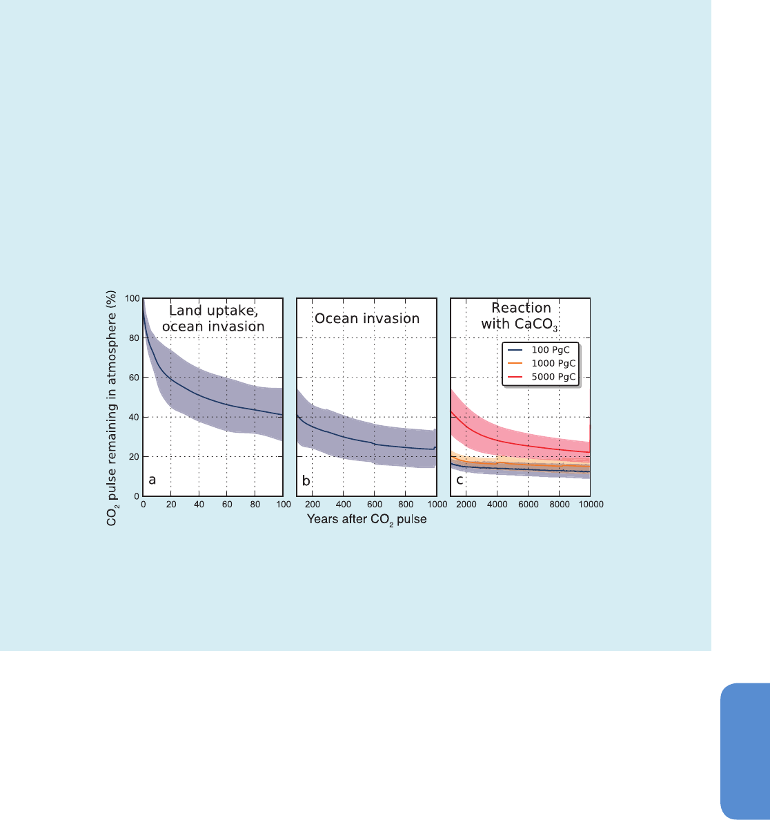
Phase 1. Within several decades of CO
2
emissions, about a third to half of an initial pulse of anthropogenic CO
2
goes into the land and
ocean, while the rest stays in the atmosphere (Box 6.1, Figure 1a). Within a few centuries, most of the anthropogenic CO
2
will be in the
form of additional dissolved inorganic carbon in the ocean, thereby decreasing ocean pH (Box 6.1, Figure 1b). Within a thousand years,
the remaining atmospheric fraction of the CO
2
emissions (see Section 6.3.2.4) is between 15 and 40%, depending on the amount of
carbon released (Archer et al., 2009b). The carbonate buffer capacity of the ocean decreases with higher CO
2
, so the larger the cumula-
tive emissions, the higher the remaining atmospheric fraction (Eby et al., 2009; Joos et al., 2013). (continued on next page)
Processes Time scale (years) Reactions
Land uptake: Photosynthesis–respiration 1–10
2
6CO
2
+ 6H
2
O + photons → C
6
H
12
O
6
+ 6O
2
C
6
H
12
O
6
+ 6O
2
→ 6CO
2
+ 6H
2
O + heat
Ocean invasion: Seawater buffer 10–10
3
CO
2
+ CO
3
2−
+ H
2
O 2HCO
3
−
Reaction with calcium carbonate 10
3
–10
4
CO
2
+ CaCO
3
+ H
2
O → Ca
2+
+ 2HCO
3
−
Silicate weathering 10
4
–10
6
CO
2
+ CaSiO
3
→ CaCO
3
+ SiO
2
Box 6.1, Table 1 | The main natural processes that remove CO
2
consecutive to a large emission pulse to the atmosphere,
their atmospheric CO
2
adjustment time scales, and main (bio)chemical reactions involved.
473
Carbon and Other Biogeochemical Cycles Chapter 6
6
6.1.1.2 Methane Cycle
CH
4
absorbs infrared radiation relatively stronger per molecule com-
pared to CO
2
(Chapter 8), and it interacts with photochemistry. On
the other hand, the methane turnover time (see Glossary) is less than
10 years in the troposphere (Prather et al., 2012; see Chapter 7). The
sources of CH
4
at the surface of the Earth (see Section 6.3.3.2) can be
thermogenic including (1) natural emissions of fossil CH
4
from geolog-
ical sources (marine and terrestrial seepages, geothermal vents and
mud volcanoes) and (2) emissions caused by leakages from fossil fuel
extraction and use (natural gas, coal and oil industry; Figure 6.2). There
are also pyrogenic sources resulting from incomplete burning of fossil
fuels and plant biomass (both natural and anthropogenic fires). The
biogenic sources include natural biogenic emissions predominantly
from wetlands, from termites and very small emissions from the ocean
(see Section 6.3.3). Anthropogenic biogenic emissions occur from rice
Box 6.1 (continued)
Phase 2. In the second stage, within a few thousands of years, the pH of the ocean that has decreased in Phase 1 will be restored by
reaction of ocean dissolved CO
2
and calcium carbonate (CaCO
3
) of sea floor sediments, partly replenishing the buffer capacity of the
ocean and further drawing down atmospheric CO
2
as a new balance is re-established between CaCO
3
sedimentation in the ocean and
terrestrial weathering (Box 6.1, Figure 1c right). This second phase will pull the remaining atmospheric CO
2
fraction down to 10 to 25%
of the original CO
2
pulse after about 10 kyr (Lenton and Britton, 2006; Montenegro et al., 2007; Ridgwell and Hargreaves, 2007; Tyrrell
et al., 2007; Archer and Brovkin, 2008).
Phase 3. In the third stage, within several hundred thousand years, the rest of the CO
2
emitted during the initial pulse will be removed
from the atmosphere by silicate weathering, a very slow process of CO
2
reaction with calcium silicate (CaSiO
3
) and other minerals of
igneous rocks (e.g., Sundquist, 1990; Walker and Kasting, 1992).
Involvement of extremely long time scale processes into the removal of a pulse of CO
2
emissions into the atmosphere complicates
comparison with the cycling of the other GHGs. This is why the concept of a single, characteristic atmospheric lifetime is not applicable
to CO
2
(Chapter 8).
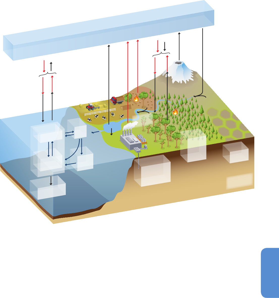
Box 6.1, Figure 1 | A percentage of emitted CO
2
remaining in the atmosphere in response to an idealised instantaneous CO
2
pulse emitted to the atmosphere in
year 0 as calculated by a range of coupled climate–carbon cycle models. (Left and middle panels, a and b) Multi-model mean (blue line) and the uncertainty interval
(±2 standard deviations, shading) simulated during 1000 years following the instantaneous pulse of 100 PgC (Joos et al., 2013). (Right panel, c) A mean of models
with oceanic and terrestrial carbon components and a maximum range of these models (shading) for instantaneous CO
2
pulse in year 0 of 100 PgC (blue), 1000 PgC
(orange) and 5000 PgC (red line) on a time interval up to 10 kyr (Archer et al., 2009b). Text at the top of the panels indicates the dominant processes that remove the
excess of CO
2
emitted in the atmosphere on the successive time scales. Note that higher pulse of CO
2
emissions leads to higher remaining CO
2
fraction (Section 6.3.2.4)
due to reduced carbonate buffer capacity of the ocean and positive climate–carbon cycle feedback (Section 6.3.2.6.6).
paddy agriculture, ruminant livestock, landfills, man-made lakes and
wetlands and waste treatment. In general, biogenic CH
4
is produced
from organic matter under low oxygen conditions by fermentation pro-
cesses of methanogenic microbes (Conrad, 1996). Atmospheric CH
4
is
removed primarily by photochemistry, through atmospheric chemistry
reactions with the OH radicals. Other smaller removal processes of
atmospheric CH
4
take place in the stratosphere through reaction with
chlorine and oxygen radicals, by oxidation in well aerated soils, and
possibly by reaction with chlorine in the marine boundary layer (Allan
et al., 2007; see Section 6.3.3.3).
A very large geological stock (globally 1500 to 7000 PgC, that is 2 x
10
6
to 9.3 x 10
6
Tg(CH
4
) in Figure 6.2; Archer (2007); with low confi-
dence in estimates) of CH
4
exists in the form of frozen hydrate deposits
(‘clathrates’) in shallow ocean sediments and on the slopes of con-
tinental shelves, and permafrost soils. These CH
4
hydrates are stable
474
Chapter 6 Carbon and Other Biogeochemical Cycles
6
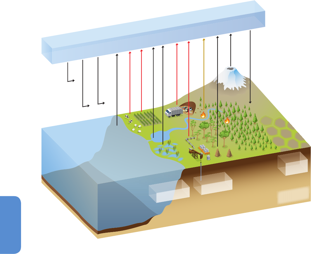
Figure 6.2 | Schematic of the global cycle of CH
4
. Numbers represent annual fluxes in Tg(CH
4
) yr
–1
estimated for the time period 2000–2009 and CH
4
reservoirs in Tg (CH
4
): the
atmosphere and three geological reservoirs (hydrates on land and in the ocean floor and gas reserves) (see Section 6.3.3). Black arrows denote ‘natural’ fluxes, that is, fluxes that
are not directly caused by human activities since 1750, red arrows anthropogenic fluxes, and the light brown arrow denotes a combined natural + anthropogenic flux. Note that
human activities (e.g., land use) may have modified indirectly the global magnitude of the natural fluxes (Section 6.3.3). Ranges represent minimum and maximum values from cited
references as given in Table 6.8 in Section 6.3.3. Gas reserves are from GEA (2006) and are consistent with numbers used by IPCC WG III for future scenarios. Hydrate reservoir sizes
are from Archer et al. (2007). The atmospheric inventories have been calculated using a conversion factor of 2.7476 TgCH
4
per ppb (Prather et al., 2012). The assumed preindustrial
annual mean globally averaged CH
4
concentration was 722 ± 25 ppb taking the average of the Antarctic Law Dome ice core observations (MacFarling-Meure et al., 2006) and the
measurements from the GRIP ice core in Greenland (Blunier et al., 1995; see also Table 2.1). The atmospheric inventory in the year 2011 is based on an annual globally averaged
CH
4
concentration of 1803 ± 4 ppb in the year 2011 (see Table 2.1). It is the sum of the atmospheric increase between 1750 and 2011 (in red) and of the pre-industrial inventory
(in black). The average atmospheric increase each year, also called growth rate, is based on a measured concentration increase of 2.2 ppb yr
–1
during the time period 2000–2009
(Dlugokencky et al., 2011).
Atmosphere 1984 + 2970 ± 45
(average atmospheric increase: 17 ±9 (Tg CH
4
yr
-1
))
Wetlands 177-284
Freshwaters 8-73
Livestock 87-94
Tropospheric OH 454-617
Rice cultivation 33-40
Termites 2-22
Hydrates 2-9
Oxidations in soils 9-47
Tropospheric CL 13-37
Stratospheric OH 16-84
Landlls and waste 67-90
Fossil fuels 85-105
Biomass burning 32-39
Geological sources
33-75
Ocean hydrates
2,000,000-8,000,000
Gas reserves
511,000-1,513,000
Permafrost
hydrates
< 530,000
Units
Fluxes: (Tg CH
4
yr
-1
)
Stocks: (Tg CH
4
)
under conditions of low temperature and high pressure. Warming or
changes in pressure could render some of these hydrates unstable with
a potential release of CH
4
to the overlying soil/ocean and/or atmos-
phere. Possible future CH
4
emissions from CH
4
released by gas hydrates
are discussed in Section 6.4.7.3.
6.1.2 Industrial Era
6.1.2.1 Carbon Dioxide and the Global Carbon Cycle
Since the beginning of the Industrial Era, humans have been produc-
ing energy by burning of fossil fuels (coal, oil and gas), a process that
is releasing large amounts of CO
2
into the atmosphere (Rotty, 1983;
Boden et al., 2011; see Section 6.3.2.1). The amount of fossil fuel CO
2
emitted to the atmosphere can be estimated with an accuracy of about
5 to 10% for recent decades from statistics of fossil fuel use (Andres et
al., 2012). Total cumulative emissions between 1750 and 2011 amount
to 375 ± 30 PgC (see Section 6.3.2.1 and Table 6.1), including a contri-
bution of 8 PgC from the production of cement.
The second major source of anthropogenic CO
2
emissions to the
atmosphere is caused by changes in land use (mainly deforestation),
which causes globally a net reduction in land carbon storage, although
recovery from past land use change can cause a net gain in in land

475
Carbon and Other Biogeochemical Cycles Chapter 6
6
carbon storage in some regions. Estimation of this CO
2
source to the
atmosphere requires knowledge of changes in land area as well as
estimates of the carbon stored per area before and after the land use
change. In addition, longer term effects, such as the decomposition of
soil organic matter after land use change, have to be taken into account
(see Section 6.3.2.2). Since 1750, anthropogenic land use changes
have resulted into about 50 million km
2
being used for cropland and
pasture, corresponding to about 38% of the total ice-free land area
(Foley et al., 2007, 2011), in contrast to an estimated cropland and pas-
ture area of 7.5 to 9 million km
2
about 1750 (Ramankutty and Foley,
1999; Goldewijk, 2001). The cumulative net CO
2
emissions from land
use changes between 1750 and 2011 are estimated at approximately
180 ± 80 PgC (see Section 6.3 and Table 6.1).
Multiple lines of evidence indicate that the observed atmospher-
ic increase in the global CO
2
concentration since 1750 (Figure 6.3)
is caused by the anthropogenic CO
2
emissions (see Section 6.3.2.3).
The rising atmospheric CO
2
content induces a disequilibrium in the
exchange fluxes between the atmosphere and the land and oceans
respectively. The rising CO
2
concentration implies a rising atmospheric
CO
2
partial pressure (pCO
2
) that induces a globally averaged net-air-
to-sea flux and thus an ocean sink for CO
2
(see Section 6.3.2.5). On
land, the rising atmospheric CO
2
concentration fosters photosynthesis
via the CO
2
fertilisation effect (see Section 6.3.2.6). However, the effi-
cacy of these oceanic and terrestrial sinks does also depend on how
the excess carbon is transformed and redistributed within these sink
reservoirs. The magnitude of the current sinks is shown in Figure 6.1
(averaged over the years 2000–2009, red arrows), together with the
cumulative reservoir content changes over the industrial era (1750–
2011, red numbers) (see Table 6.1, Section 6.3).
6.1.2.2 Methane Cycle
After 1750, atmospheric CH
4
levels rose almost exponentially with
time, reaching 1650 ppb by the mid-1980s and 1803 ppb by 2011.
Between the mid-1980s and the mid-2000s the atmospheric growth
of CH
4
declined to nearly zero (see Section 6.3.3.1, see also Chapter
2). More recently since 2006, atmospheric CH
4
is observed to increase
again (Rigby et al., 2008); however, it is unclear if this is a short-term
fluctuation or a new regime for the CH
4
cycle (Dlugokencky et al., 2009).
There is very high level of confidence that the atmospheric CH
4
increase during the Industrial Era is caused by anthropogenic activities.
The massive increase in the number of ruminants (Barnosky, 2008),
the emissions from fossil fuel extraction and use, the expansion of rice
paddy agriculture and the emissions from landfills and waste are the
dominant anthropogenic CH
4
sources. Total anthropogenic sources
contribute at present between 50 and 65% of the total CH
4
sources
(see Section 6.3.3). The dominance of CH
4
emissions located mostly in
the NH (wetlands and anthropogenic emissions) is evidenced by the
observed positive north–south gradient in CH
4
concentrations (Figure
6.3). Satellite-based CH
4
concentration measurements averaged over
the entire atmospheric column also indicate higher concentrations of
CH
4
above and downwind of densely populated and intensive agricul-
ture areas where anthropogenic emissions occur (Frankenberg et al.,
2011).
6.1.3 Connections Between Carbon and the Nitrogen
and Oxygen Cycles
6.1.3.1 Global Nitrogen Cycle Including Nitrous Oxide
The biogeochemical cycles of nitrogen and carbon are tightly coupled
with each other owing to the metabolic needs of organisms for these
two elements. Changes in the availability of one element will influence
not only biological productivity but also availability and requirements
for the other element (Gruber and Galloway, 2008) and in the longer
term, the structure and functioning of ecosystems as well.
Before the Industrial Era, the creation of reactive nitrogen Nr (all nitro-
gen species other than N
2
) from non-reactive atmospheric N
2
occurred
primarily through two natural processes: lightning and biological
nitrogen fixation (BNF). BNF is a set of reactions that convert N
2
to
ammonia in a microbially mediated process. This input of Nr to the
land and ocean biosphere was in balance with the loss of Nr though
denitrification, a process that returns N
2
back to the atmosphere (Ayres
et al., 1994). This equilibrium has been broken since the beginning of
the Industrial Era. Nr is produced by human activities and delivered to
ecosystems. During the last decades, the production of Nr by humans
has been much greater than the natural production (Figure 6.4a; Sec-
tion 6.3.4.3). There are three main anthropogenic sources of Nr: (1) the
Haber-Bosch industrial process, used to make NH
3
from N
2
, for nitrogen
fertilisers and as a feedstock for some industries; (2) the cultivation of
legumes and other crops, which increases BNF; and (3) the combustion
of fossil fuels, which converts atmospheric N
2
and fossil fuel nitrogen
into nitrogen oxides (NO
x
) emitted to the atmosphere and re-deposited
at the surface (Figure 6.4a). In addition, there is a small flux from the
mobilization of sequestered Nr from nitrogen-rich sedimentary rocks
(Morford et al., 2011) (not shown in Figure 6.4a).
The amount of anthropogenic Nr converted back to non-reactive N
2
by
denitrification is much smaller than the amount of Nr produced each
year, that is, about 30 to 60% of the total Nr production, with a large
uncertainty (Galloway et al., 2004; Canfield et al., 2010; Bouwman et
al., 2013). What is more certain is the amount of N
2
O emitted to the
atmosphere. Anthropogenic sources of N
2
O are about the same size
as natural terrestrial sources (see Section 6.3.4 and Table 6.9 for the
global N
2
O budget). In addition, emissions of Nr to the atmosphere,
as NH
3
and NO
x
, are caused by agriculture and fossil fuel combustion.
A portion of the emitted NH
3
and NO
x
is deposited over the conti-
nents, while the rest gets transported by winds and deposited over
the oceans. This atmospheric deposition flux of Nr over the oceans is
comparable to the flux going from soils to rivers and delivered to the
coastal ocean (Galloway et al., 2004; Suntharalingam et al., 2012).
The increase of Nr creation during the Industrial Era, the connections
among its impacts, including on climate and the connections with the
carbon cycle are presented in Box 6.2.
For the global ocean, the best BNF estimate is 160 TgN yr
–1
, which
is roughly the midpoint of the minimum estimate of 140 TgN yr
–1
of
Deutsch et al. (2007) and the maximum estimate of 177 TgN yr
–1
(Gro-
szkopf et al., 2012). The probability that this estimate will need an
upward revision in the near future is high because several additional
processes are not yet considered (Voss et al., 2013).
476
Chapter 6 Carbon and Other Biogeochemical Cycles
6
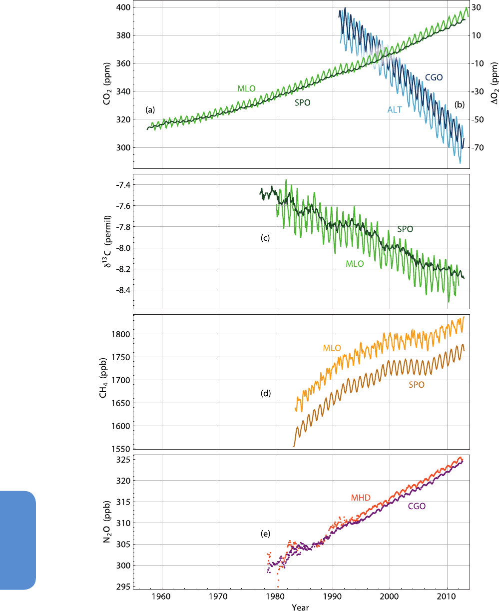
Figure 6.3 | Atmospheric concentration of CO
2
, oxygen,
13
C/
12
C stable isotope ratio in CO
2
, CH
4
and N
2
O recorded over the last decades at representative stations (a) CO
2
from
Mauna Loa (MLO) Northern Hemisphere and South Pole Southern Hemisphere (SPO) atmospheric stations (Keeling et al., 2005). (b) O
2
from Alert Northern Hemisphere (ALT) and
Cape Grim Southern Hemisphere (CGO) stations (http://scrippso2.ucsd.edu/ right axes, expressed relative to a reference standard value). (c)
13
C/
12
C: Mauna Loa, South Pole (Keeling
et al., 2005). (d) CH
4
from Mauna Loa and South Pole stations (Dlugokencky et al., 2012). (e) N
2
O from Mace-Head Northern Hemisphere (MHD) and Cape Grim stations (Prinn et
al., 2000).
477
Carbon and Other Biogeochemical Cycles Chapter 6
6
Box 6.2 | Nitrogen Cycle and Climate-Carbon Cycle Feedbacks
Human creation of reactive nitrogen by the Haber–Bosch process (see Sections 6.1.3 and 6.3.4), fossil fuel combustion and agricultural
biological nitrogen fixation (BNF) dominate Nr creation relative to biological nitrogen fixation in natural terrestrial ecosystems. This
dominance impacts on the radiation balance of the Earth (covered by the IPCC; see, e.g., Chapters 7 and 8), and affects human health
and ecosystem health as well (EPA, 2011b; Sutton et al., 2011).
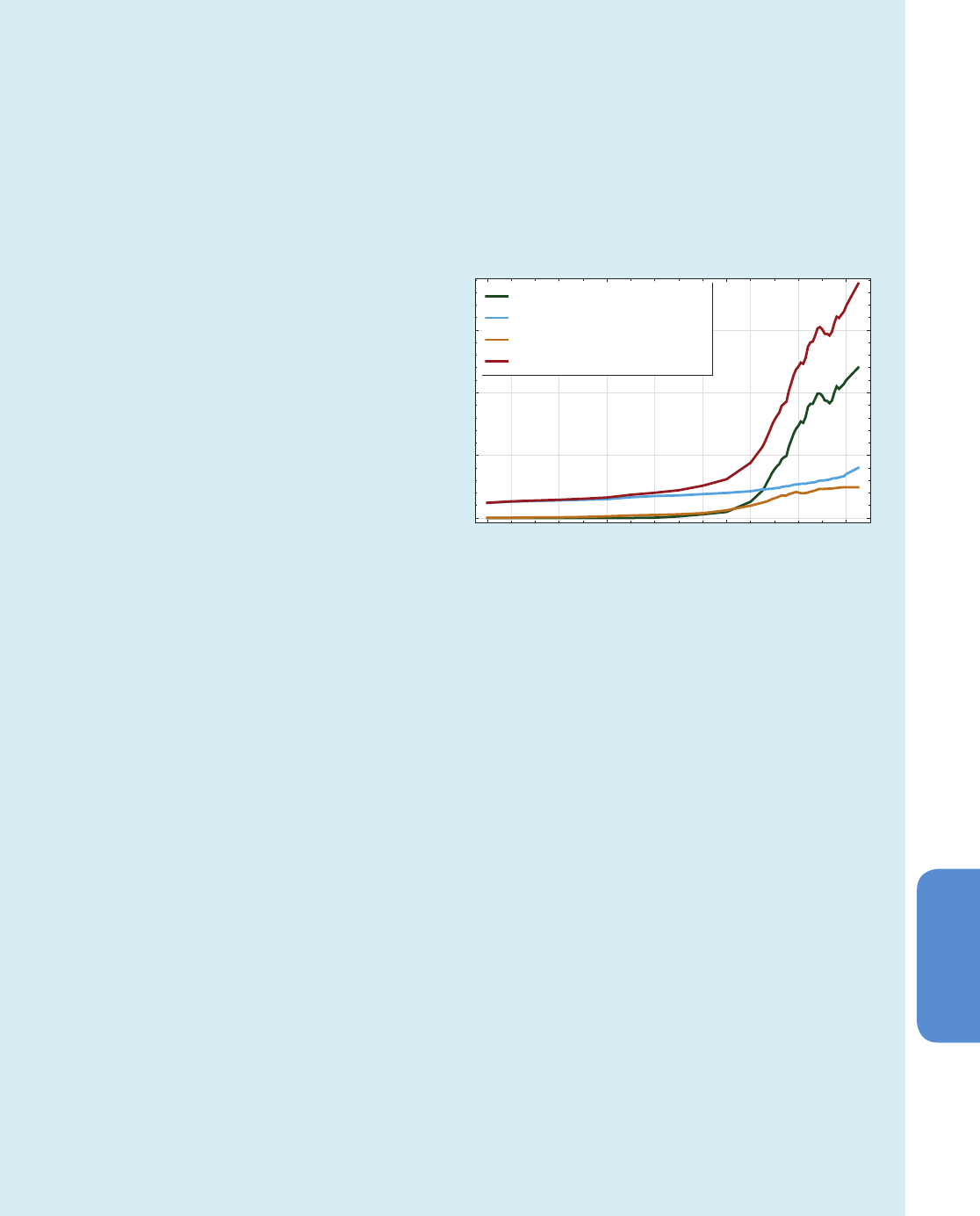
The Nr creation from 1850 to 2005 is shown in Box 6.2 (Figure 1). After mid-1970s, human production of Nr exceeded natural production.
During the 2000s food production (mineral fertilisers, legumes) accounts for three-quarters of Nr created by humans, with fossil fuel
combustion and industrial uses accounting equally for the remainder (Galloway et al., 2008; Canfield et al., 2010; Sutton et al., 2011).
The three most relevant questions regarding the anthro-
pogenic perturbation of the nitrogen cycle with respect to
global change are: (1) What are the interactions with the
carbon cycle, and the effects on carbon sinks (see Sections
6.3.2.6.5 and 6.4.2.1), (2) What are the effects of increased
Nr on the radiative forcing of nitrate aerosols (Chapter 7,
7.3.2) and tropospheric ozone (Chapters 8), (3) What are
the impacts of the excess of Nr on humans and ecosystems
(health, biodiversity, eutrophication, not treated in this
report, but see, for example, EPA, 2011b; Sutton et al., 2011).
Essentially all of the Nr formed by human activity is spread
into the environment, either at the point of creation (i.e.,
fossil fuel combustion) or after it is used in food production
and in industry. Once in the environment, Nr has a number
of negative impacts if not converted back into N
2
. In addi-
tion to its contributions to climate change and stratospheric
ozone depletion, Nr contributes to the formation of smog;
increases the haziness of the troposphere; contributes to the
acidification of soils and freshwaters; and increases the pro-
ductivity in forests, grasslands, open and coastal waters and
open ocean, which can lead to eutrophication and reduction
in biodiversity in terrestrial and aquatic ecosystems. In addition, Nr-induced increases in nitrogen oxides, aerosols, tropospheric ozone,
and nitrates in drinking water have negative impacts on human health (Galloway et al., 2008; Davidson et al., 2012). Once the nitrogen
atoms become reactive (e.g., NH
3
, NO
x
), any given Nr atom can contribute to all of the impacts noted above in sequence. This is called the
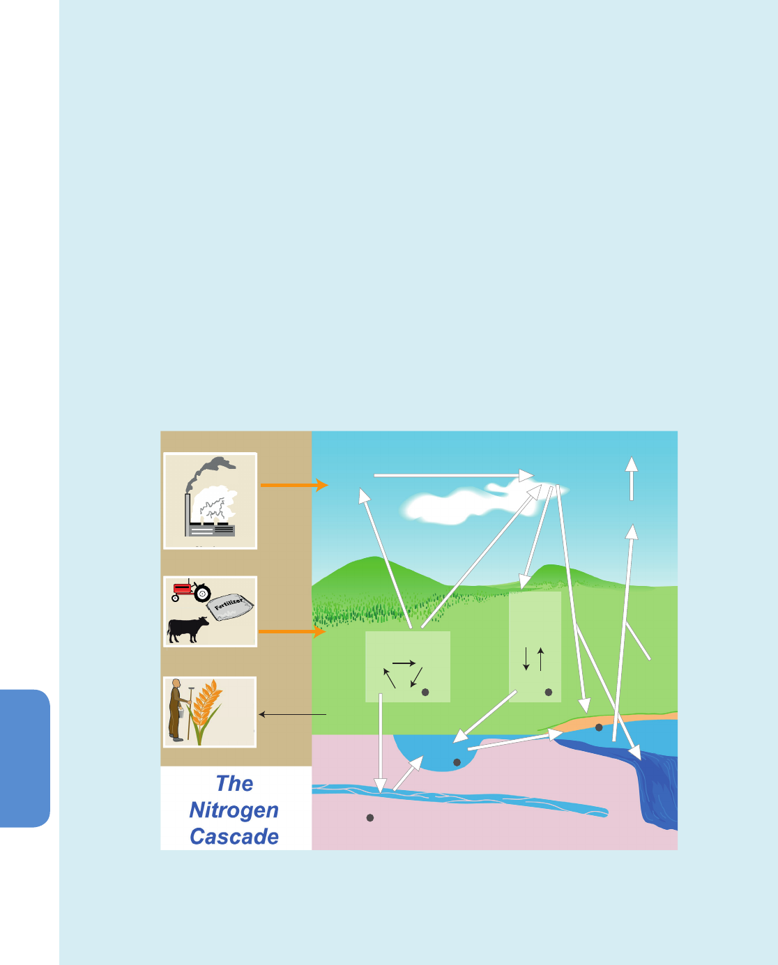
nitrogen cascade (Galloway et al., 2003; Box 6.2, Figure 2). The nitrogen cascade is the sequential transfer of the same Nr atom through
the atmosphere, terrestrial ecosystems, freshwater ecosystems and marine ecosystems that results in multiple effects in each reservoir.
Because of the nitrogen cascade, the creation of any molecule of Nr from N
2
, at any location, has the potential to affect climate, either
directly or indirectly, as explained in this box This potential exists until the Nr gets converted back to N
2
.
The most important processes causing direct links between anthropogenic Nr and climate change include(Erisman et al., 2011): (1)
N
2
O formation during industrial processes (e.g., fertiliser production), combustion, or microbial conversion of substrate containing
nitrogen—notably after fertiliser and manure application to soils. N
2
O is a strong greenhouse gas (GHG), (2) emission of anthropogenic
NO
x
leading to (a) formation of tropospheric O
3
, (which is the third most important GHG), (b) a decrease of CH
4
and (c) the formation of
nitrate aerosols.Aerosol formation affects radiative forcing, as nitrogen-containing aerosols have a direct cooling effect in addition to
an indirect cooling effect through cloud formation and (3)NH
3
emission to the atmosphere which contributes to aerosol formation.The
first process has a warming effect. The second has both a warming (as a GHG) and a cooling (through the formation of the OH radical
in the troposphere which reacts with CH
4
,and through aerosol formation) effect. The net effect of all three NO
x
-related contributions is
cooling.The third process has a cooling effect.
The most important processes causing an indirect link between anthropogenic Nr and climate change include: (1)
nitrogen-dependent changes in soil organic matter decomposition and hence CO
2
emissions, affecting heterotrophic respiration;
(2) alteration of the biospheric CO
2
sink due to increased supply of Nr. About half of the carbon that is emitted to the atmosphere is
1850 1900 1950 2000
0
50
100
150
Year
Total Nr Creation
Fossil Fuel Burning
Biological Nitrogen Fixation
Haber Bosch Process
Nr Creation (TgN yr
-1
)
Box 6.2, Figure 1 | Anthropogenic reactive nitrogen (Nr) creation rates (in TgN yr
–1
)
from fossil fuel burning (orange line), cultivation-induced biological nitrogen fixation
(blue line), Haber–Bosch process (green line) and total creation (red line). Source:
Galloway et al. (2003), Galloway et al. (2008). Note that updates are given in Table
6.9. The only one with significant changes in the more recent literature is cultivation-
induced BNF) which Herridge et al. (2008) estimated to be 60 TgN yr
–1
. The data are
only reported since 1850, as no published estimate is available since 1750.
(continued on next page)
478
Chapter 6 Carbon and Other Biogeochemical Cycles
6
taken up by the biosphere; Nr affects net CO
2
uptake from the atmosphere in terrestrial systems, rivers, estuaries and the open ocean in
a positive direction (by increasing productivity or reducing the rate of organic matter breakdown) and negative direction (in situations
where it accelerates organic matter breakdown). CO
2
uptake in the ocean causes ocean acidification, which reduces CO
2
uptake; (3)
changes in marine primary productivity, generally an increase, in response to Nr deposition; and (4) O
3
formed in the troposphere as a
result of NO
x
and volatile organic compound emissions reduces plant productivity, and therefore reduces CO
2
uptake from the atmos-
phere. On the global scale the net influence of the direct and indirect contributions of Nr on the radiative balance was estimated to be
–0.24 W m
–2
(with an uncertainty range of +0.2 to –0.5 W m
–2
)(Erisman et al., 2011).
Nr is required for both plants and soil microorganisms to grow, and plant and microbial processes play important roles in the global
carbon cycle. The increasing concentration of atmospheric CO
2
is observed to increase plant photosynthesis (see Box 6.3) and plant
growth, which drives an increase of carbon storage in terrestrial ecosystems. Plant growth is, however, constrained by the availability
of Nr in soils (see Section 6.3.2.6.5). This means that in some nitrogen-poor ecosystems, insufficient Nr availability will limit carbon
sinks, while the deposition of Nr may instead alleviate this limitation and enable larger carbon sinks (see Section 6.3.2.6.5). Therefore,
human production of Nr has the potential to mitigate CO
2
emissions by providing additional nutrients for plant growth in some regions.
Microbial growth can also be limited by the availability of Nr, particularly in cold, wet environments, so that human production of Nr
also has the potential to accelerate the decomposition of organic matter, increasing release of CO
2
. The availability of Nr also changes
in response to climate change, generally increasing with warmer temperatures and increased precipitation (see Section 6.4.2.1), but
with complex interactions in the case of seasonally inundated environments. This complex network of feedbacks is amenable to study
through observation and experimentation (Section 6.3) and Earth System modelling (Section 6.4). Even though we do not yet have a
thorough understanding of how nitrogen and carbon cycling will interact with climate change, elevated CO
2
and human Nr production
in the future, given scenarios of human activity, current observations and model results all indicate that low nitrogen availability will
limit carbon storage on land in the 21st century (see Section 6.4.2.1).
Atmosphere
Ozone
Eects
Stratospheric
Eects
Particulate
Matter
Eects
Greenhouse
Eects
Terrestrial
Ecosystems
Aquatic Ecosystem
Groundwater
Eects
Surface Water
Eects
Ocean
Eects
Coastal
Eects
Agro-ecosystem
Eects
CropAnimal
Soil
Forest &
Grassland
Eects
Plant
Soil
NH
x
NO
y
N
2
O
(land)
NH
x
NO
y
NO
x
NH
3
NH
x
N
2
O
N
2
O
N
organic
N
2
O
(water)
NO
3
-
NO
x
Food
production
People
(food; ber)
Energy production
Box 6.2, Figure 2 | Illustration of the nitrogen cascade showing the sequential effects that a single atom of nitrogen in its various molecular forms can have in various
reservoirs after it has been converted from nonreactive N
2
to a reactive form by energy and food production (orange arrows). Once created the reactive nitrogen has
the potential to continue to contribute to impacts until it is converted back to N
2
. The small black circle indicates that there is the potential for denitrification to occur
within that reservoir. NH
3
= ammonia; NH
x
= ammonia plus ammonium; NO
3
–
= nitrate; NO
x
= nitrogen oxides; NO
y
= NO
x
and other combinations of nitrogen and
oxygen (except N
2
O); N
2
O = nitrous oxide. (Adapted with permission from the GEO Yearbook 2003, United Nations Environmental Programme (UNEP), 2004 which
was based on Galloway et al., 2003.)
Box 6.2 (continued)
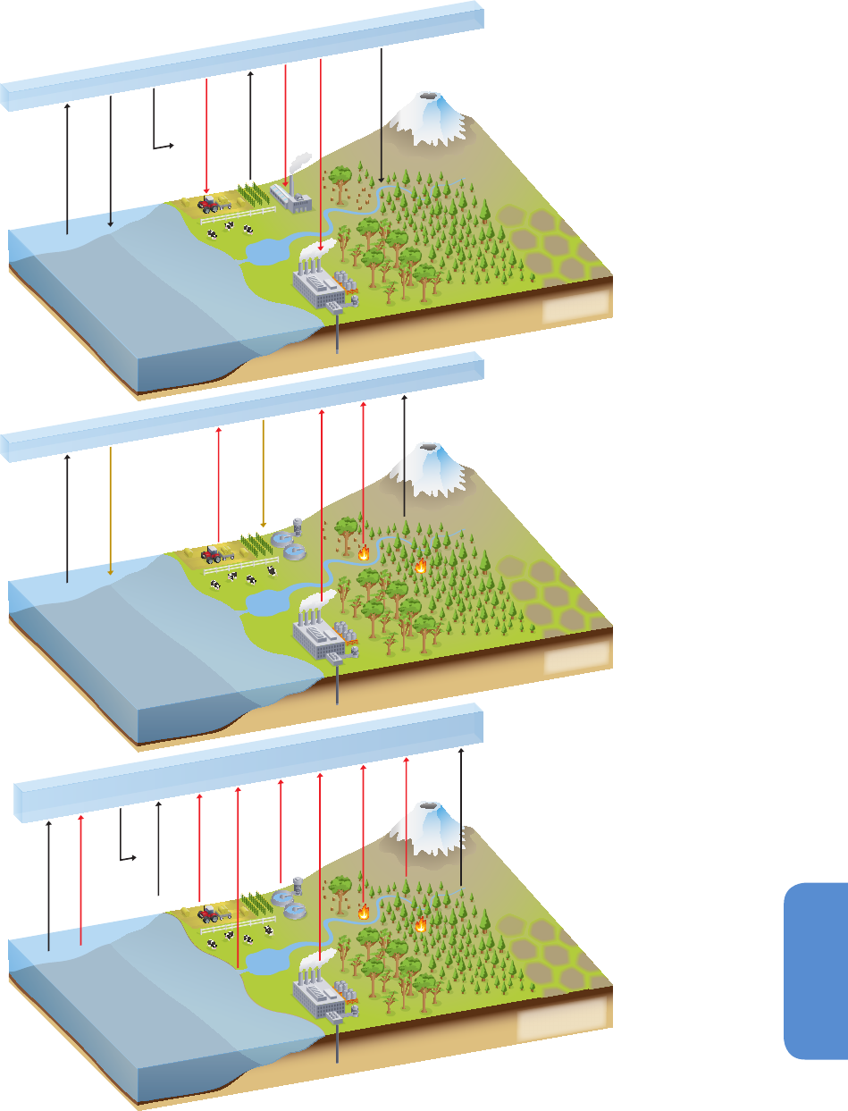
479
Carbon and Other Biogeochemical Cycles Chapter 6
6
Atmosphere: N
2
O (1340 + 213 ±50)
(average atmospheric increase: 3.6 ±0.15 (Tg N [N
2
O] yr
-1
))
0.2 (0.1-0.4)From atmospheric
deposition on ocean
0.6 (0.1-2.9)
Rivers, estuaries,
coastal zone
Agriculture 4.1 (1.7-4.8)
Human excreta 0.2 (0.1-0.3)
0.7 (0.2-1.0)Biomass and
biofuel burning
0.4 (0.3-0.9)From atmospheric
deposition on land
0.7 (0.2-1.8)Fossil fuels and
industry
6.6 (3.3-9.0)
Soils under natural
vegetation
Oceans 3.8 (1.8-9.4)
0.6 (0.3-1.2)Atmospheric
chemistry
Units
Fluxes: (Tg N [N
2
O] yr
-1
)
Stocks: (Tg N [N
2
O] yr
-1
)
Stratospheric sink 14.3 (4.3-27.2)
Atmosphere: Reactive nitrogen species (except N
2
O)
Deposition 20 (NOy)
17 (NHx)
36 (NHx)
Deposition 27 (NOy)
4 (NOx)
NH
3
emission,
agriculture and
sewage
30 (NH
3
)
9 (NH
3
)
6 (NOx)Biomass and
biofuel burning
0.5 (NH
3
)
28 (NOx)NOx emission, fossil fuel
combustion and
industrial processes
2 (NH
3
)
7 (NOx)Soils under natural
vegetation
NH
3
emission 8.2
Units
Fluxes: (Tg N yr
-1
)
Units
Fluxes: (Tg N yr
-1
)
Atmospheric molecular Nitrogen (N
2
)
60 (50-70)
Cultivation
xation
124 (117-126) Industrial
xation
30 (27-33)
Fossil fuel
combustion
160 (140-177)Biological
xation
Lightining 4 (3-5)
Denitrication 300 (200-400)
Denitrication 109 (101-118)
58 (50-100)
Natural biological
xation
(Haber Bosch)
a)
b)
c)
Figure 6.4 | Schematic of the global nitrogen cycle. (a) The natural and anthropogenic processes that create reactive nitrogen and the corresponding rates of denitrification that
convert reactive nitrogen back to N
2
. (b) The flows of the reactive nitrogen species NO
y
and NH
x
. (c) The stratospheric sink of N
2
O is the sum of losses via photolysis and reaction
with O(1D) (oxygen radical in the 1D excited state; Table 6.9). The global magnitude of this sink is adjusted here in order to be equal to the difference between the total sources
and the observed growth rate. This value falls within literature estimates (Volk et al., 1997). The atmospheric inventories have been calculated using a conversion factor of 4.79 TgN
(N
2
O) per ppb (Prather et al., 2012).

480
Chapter 6 Carbon and Other Biogeochemical Cycles
6
A global denitrification rate is much more difficult to constrain than
the BNF considering the changing paradigms of nitrogen cycling in the
oxygen minimum zones or the unconstrained losses in permeable sed-
iments on the continental shelves (Gao et al., 2012). The coastal ocean
may have losses in the range of 100 to 250 (Voss et al., 2011). For the
open and distal ocean Codispoti (2007) estimated an upper limit of
denitrification of 400 TgN yr
–1
. Voss et al. (2013) used a conservative
estimate of 100 TgN yr
–1
for the coastal ocean, and 200 to 300 TgN yr
–1
for the open ocean. Because the upper limit in the global ocean is 400
TgN yr
–1
, 300 ± 100 TgN yr
–1
is the best estimate for global ocean losses
of reactive nitrogen (Table 6.9).
This chapter does not describe the phosphorus and sulphur biogeo-
chemical cycles, but phosphorus limitations on carbon sinks are briefly
addressed in Section 6.4.8.2 and future sulphur deposition in Section
6.4.6.2.
6.1.3.2 Oxygen
Atmospheric oxygen is tightly coupled with the global carbon cycle
(sometimes called a mirror of the carbon cycle). The burning of fossil
fuels removes oxygen from the atmosphere in a tightly defined stoichi-
ometric ratio depending on fuel carbon content. As a consequence of
the burning of fossil fuels, atmospheric O
2
levels have been observed
to decrease steadily over the last 20 years (Keeling and Shertz, 1992;
Manning and Keeling, 2006) (Figure 6.3b). Compared to the atmos-
pheric oxygen content of about 21% this decrease is very small; how-
ever, it provides independent evidence that the rise in CO
2
must be due
to an oxidation process, that is, fossil fuel combustion and/or organic
carbon oxidation, and is not caused by, for example, volcanic emissions
or by outgassing of dissolved CO
2
from a warming ocean. The atmos-
pheric oxygen measurements furthermore also show the north–south
concentration O
2
difference (higher in the south and mirroring the CO
2
north–south concentration difference) as expected from the stronger
fossil fuel consumption in the NH (Keeling et al., 1996).
On land, during photosynthesis and respiration, O
2
and CO
2
are
exchanged in nearly a 1:1 ratio. However, with respect to exchanges
with the ocean, O
2
behaves quite differently from CO
2
, because com-
pared to the atmosphere only a small amount of O
2
is dissolved in the
ocean whereas by contrast the oceanic CO
2
content is much larger due
to the carbonate chemistry. This different behaviour of the two gases
with respect to ocean exchange provides a powerful method to assess
independently the partitioning of the uptake of anthropogenic CO
2
by
land and ocean (Manning and Keeling, 2006), Section 6.3.2.3.
6.2 Variations in Carbon and Other
Biogeochemical Cycles Before the Fossil
Fuel Era
The Earth System mechanisms that were responsible for past variations
in atmospheric CO
2
, CH
4
, and N
2
O will probably operate in the future
as well. Past archives of GHGs and climate therefore provide useful
knowledge, including constraints for biogeochemical models applied
to the future projections described in Section 6.4. In addition, past
archives of GHGs also show with very high confidence that the average
rates of increase of CO
2
, CH
4
and N
2
O are larger during the Industrial
Era (see Section 6.3) than during any comparable period of at least the
past 22,000 years (Joos and Spahni, 2008).
6.2.1 Glacial–Interglacial Greenhouse Gas Changes
6.2.1.1 Processes Controlling Glacial Carbon Dioxide
Ice cores recovered from the Antarctic ice sheet reveal that the con-
centration of atmospheric CO
2
at the Last Glacial Maximum (LGM; see
Glossary) at 21 ka was about one third lower than during the sub-
sequent interglacial (Holocene) period started at 11.7 ka (Delmas et
al., 1980; Neftel et al., 1982; Monnin et al., 2001). Longer (to 800 ka)
records exhibit similar features, with CO
2
values of ~180 to 200 ppm
during glacial intervals (Petit et al., 1999). Prior to 420 ka, interglacial
CO
2
values were 240 to 260 ppm rather than 270 to 290 ppm after that
date (Lüthi et al., 2008).
A variety of proxy reconstructions as well as models of different com-
plexity from conceptual to complex Earth System Models (ESM; see
Glossary) have been used to test hypotheses for the cause of lower
LGM atmospheric CO
2
concentrations (e.g., Köhler et al., 2005; Sigman
et al., 2010). The mechanisms of the carbon cycle during the LGM
which lead to low atmospheric CO
2
can be broken down by individual
drivers (Figure 6.5). It should be recognized, however, that this sep-
aration is potentially misleading, as many of the component drivers
shown in Figure 6.5 may combine nonlinearly (Bouttes et al., 2011).
Only well-established individual drivers are quantified (Figure 6.5), and
discussed here.
6.2.1.1.1 Reduced land carbon
Despite local evidence of larger carbon storage in permafrost regions
during glacial periods (Zimov et al., 2009; Zech et al., 2011), the δ
13
C
record of ocean waters as preserved in benthic foraminiferal shells has
been used to infer that global terrestrial carbon storage was reduced
in glacial times, thus opposite to recorded changes in atmospheric CO
2
.
Data-based estimates of the deficit between LGM and pre-industrial
land carbon storage range from a few hundreds to 1000 PgC (e.g.,
Bird et al., 1996; Ciais et al., 2012). Dynamic vegetation models tend
to simulate values at the higher end (~800 PgC) (Kaplan et al., 2002;
Otto et al., 2002) and indicate a role for the physiological effects of low
CO
2
on photosynthesis at the LGM at least as large as that of colder
and dryer climate conditions in determining the past extent of forests
(Prentice and Harrison, 2009).
6.2.1.1.2 Lower sea surface temperatures
Reconstructions of sea surface temperatures (SSTs) during the LGM
suggest that the global surface ocean was on average 3°C to 5°C
cooler compared to the Holocene. Because the solubility of CO
2
increases at colder temperature (Zeebe and Wolf-Gladrow, 2001), a
colder glacial ocean will hold more carbon. However, uncertainty in
reconstructing the LGM pattern of ocean temperature, particularly
in the tropics (Archer et al., 2000; Waelbroeck et al., 2009), together
with problems in transforming this pattern to the resolution of models
in light of the nonlinear nature of the CO
2
–temperature relationship

481
Carbon and Other Biogeochemical Cycles Chapter 6
6
(Ridgwell, 2001), creates a large spread in modelled estimates, Most
ocean general circulation models (OGCM) projections, however, cluster
more tightly and suggest that lower ocean temperatures contribute to
lower CO
2
values by 25 ppm during the LGM (Figure 6.5).
6.2.1.1.3 Lower sea level and increased salinity
During the LGM, sea level was about ~120 m lower than today, and
this change in ocean volume had several well-understood effects on
atmospheric CO
2
concentrations. Lower sea level impacts the LGM
ocean carbon cycle in two main ways. First, the resulting higher LGM
ocean surface salinity causes atmospheric CO
2
to be higher than during
the Holocene. Second, the total dissolved inorganic carbon and alka-
linity (a measure of the capacity of an aqueous solution to neutralize
acid) become more concentrated in equal proportions, and this process
also causes atmospheric CO
2
to be higher during the LGM. In total,
lower sea level is estimated to contribute to higher CO
2
values by 15
ppm during the LGM (Figure 6.5), implying that other processes must
explain the lower CO
2
values measured in ice cores.
6.2.1.1.4 Ocean circulation and sea ice
Reorganization in ocean circulation during glacial periods that pro-
moted the retention of dissolved inorganic carbon in the deep ocean
during the LGM has become the focus of most research on the gla-
cial–interglacial CO
2
problem. That ocean circulation plays a key role in
low glacial period atmospheric CO
2
concentration is exemplified by the
tight coupling observed between reconstructed deep ocean tempera-
tures and atmospheric CO
2
(Shackleton, 2000). Evidence from marine
bore hole sites (Adkins et al., 2002) and from marine sediment cores
(Jaccard et al., 2005; Skinner et al., 2010) show that the glacial ocean
was highly stratified compared to interglacial conditions and may thus
have held a larger store of carbon during glacial times. δ
13
CO
2
ice core
records (Lourantou et al., 2010a, 2010b; Schmitt et al., 2012), as well
as radiocarbon records from deep-sea corals demonstrate the role of
a deep and stratified Southern Ocean in the higher LGM ocean carbon
storage. However, conflicting hypotheses exist on the drivers of this
increase in the Southern Ocean stratification, for example, northward
shift and weakening of Southern Hemisphere (SH) westerly winds (Tog-
gweiler et al., 2006), reduced air–sea buoyancy fluxes (Watson and
Garabato, 2006) or massive brine rejections during sea ice formation
(Bouttes et al., 2011, 2012). Ocean carbon cycle models have simulated
a circulation-induced effect on LGM CO
2
that can explain lower values
than during interglacial by 3 ppm (Bopp et al., 2003) to 57 ppm (Tog-
gweiler, 1999).
A long-standing hypothesis is that increased LGM sea ice cover acted
as a barrier to air–sea gas exchange and hence reduced the ‘leakage’
of CO
2
during winter months from the ocean to the atmosphere during
glacial periods (Broecker and Peng, 1986). However, concurrent chang-
es in ocean circulation and biological productivity complicate the esti-
mation of the impact of increased sea ice extent on LGM atmospher-
ic CO
2
(Kurahashi-Nakamura et al., 2007). With the exception of the
results of an idealised box model (Stephens and Keeling, 2000), ocean
carbon models are relatively consistent in projecting a small effect of
higher sea ice extent on maintaining atmospheric CO
2
lower during
LGM (Archer et al., 2003).
6.2.1.1.5 Iron fertilisation
Both marine and terrestrial sediment records indicate higher rates of
deposition of dust and hence iron (Fe) supply at the LGM (Mahow-
ald et al., 2006), implying a potential link between Fe fertilisation of
marine productivity and lower glacial CO
2
(Martin, 1990). However,
despite the fact that ocean carbon cycle models generally employ sim-
ilar reconstructions of glacial dust fluxes (i.e., Mahowald et al., 1999;
Mahowald et al., 2006), there is considerable disagreement among
them in the associated CO
2
change. OGCM that include a descrip-
tion of the Fe cycle tend to cluster at the lower end of simulated CO
2
changes between glacial and interglacial (e.g., Archer at al., 2000;
Bopp et al., 2003), whereas box models (e.g., Watson et al., 2000) or
Earth System Models of Intermediate Complexity (EMICs, e.g., Brovkin
et al., 2007) tend to produce CO
2
changes which are at the higher
end (Parekh et al., 2008). An alternative view comes from inferences
drawn from the timing and magnitude of changes in dust and CO
2
in
ice cores (Röthlisberger et al., 2004), assigning a 20 ppm limit for the
lowering of CO
2
during the LGM in response to an Southern Ocean Fe
fertilisation effect, and a 8 ppm limit for the same effect in the North
Pacific.
6.2.1.1.6 Other glacial carbon dioxide drivers
A number of further aspects of altered climate and biogeochemistry
at the LGM are also likely to have affected atmospheric CO
2
. Reduced
bacterial metabolic rates and remineralization (see Glossary) of organ-
ic matter (Matsumoto, 2007; Menviel et al., 2012), increased glacial
supply of dissolved silica (required by diatoms to form frustules)
(Harrison, 2000), ‘silica leakage’ (Brzezinski et al., 2002; Matsumoto
et al., 2002), changes in net global weathering rates (Berner, 1992;
Munhoven, 2002), reduction in coral reef growth and other forms of
shallow water CaCO
3
accumulation (Berger, 1982), carbonate com-
pensation (Ridgwell and Zeebe, 2005) and changes in the CaCO
3
to
organic matter ‘rain ratio’ to the sediments (Archer and Maier-Reimer,
1994) will act to amplify or diminish the effect of many of the afore-
mentioned drivers on glacial CO
2
.
6.2.1.1.7 Summary
All of the major drivers of the glacial-to-interglacial atmospheric
CO
2
changes (Figure 6.5) are likely to have already been identified.
However, Earth System Models have been unable to reproduce the
full magnitude of the glacial-to-interglacial CO
2
changes. Significant
uncertainties exist in glacial boundary conditions and on some of the
primary controls on carbon storage in the ocean and in the land. These
uncertainties prevent an unambiguous attribution of individual mech-
anisms as controllers of the low glacial CO
2
concentrations. Further
assessments of the interplay of different mechanisms prior to degla-
cial transitions or in glacial inceptions will provide additional insights
into the drivers and processes that caused the glacial decrease of CO
2
.
Because several of these identified drivers (e.g., organic matter rem-
ineralization, ocean stratification) are sensitive to climate change in
general, improved understanding drawn from the glacial–interglacial
cycles will help constrain the magnitude of future ocean feedbacks
on atmospheric CO
2
. Other drivers (e.g., iron fertilisation) are involved
in geoengineering methods (see Glossary), such that improved under-
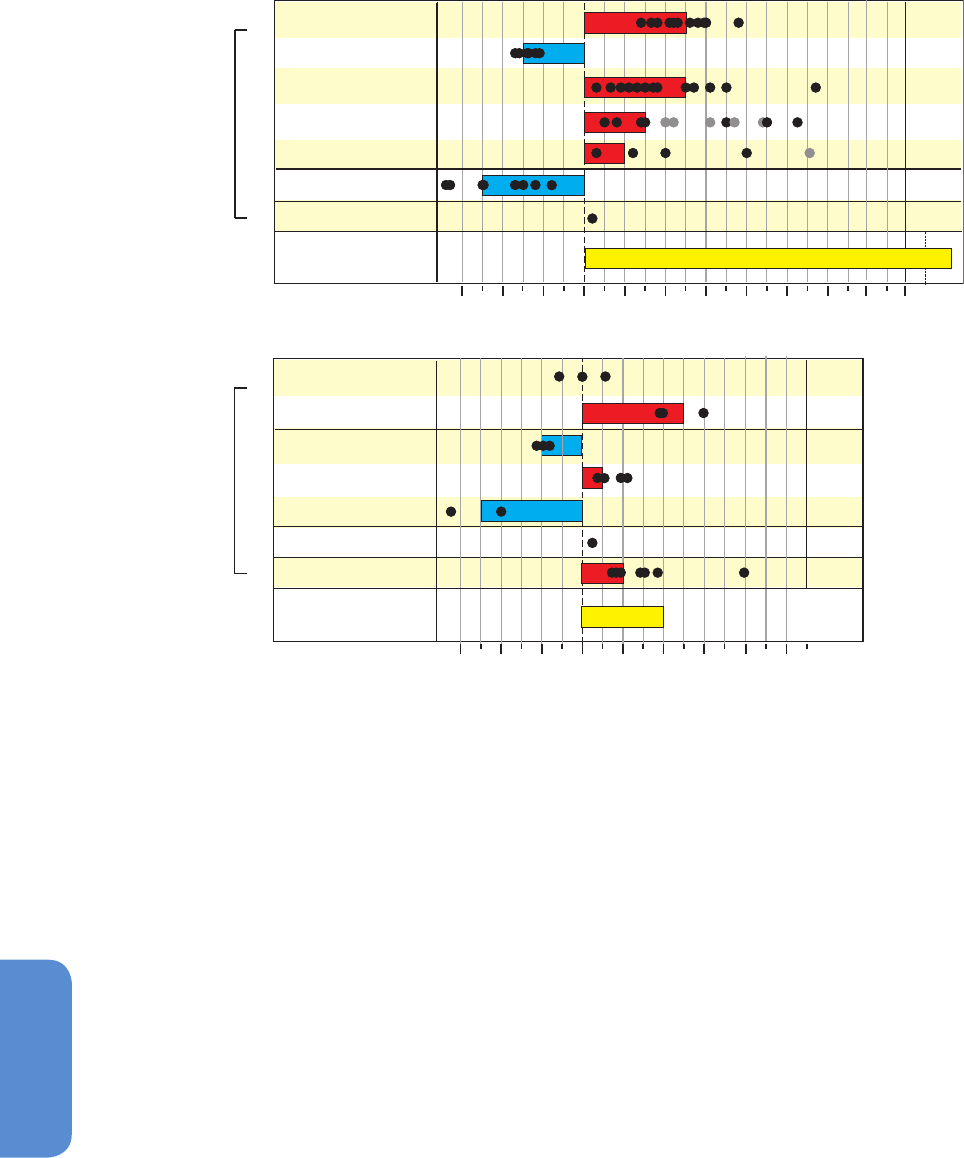
482
Chapter 6 Carbon and Other Biogeochemical Cycles
6
0103020-10-20-3
07
080
sea-level and salinity
H
CO2 fertilisation
& biome shifts
CO
2
change (ppm)
sea surface
temperature
Fe fertilisation
terrestrial weathering
coral reef & carbonate
compensation
ocean circulation
Ocean LandGeol.
H
M
M
M
H
L
Data
Glacial to Interglacial
ice-core
record
Drivers
land use
Holocene
20 ka to 0 ka
40 50 60
0103020-10-20-30
CO
2
fertilisation
sea surface
temperature
coral reef & carbonate
compensation
Ocean LandGeol.Data
ice-core
record
Drivers
40 50
peat accumulation
volcanic outgassing
Human
7 ka to 0 ka *
L
M
M
M
L
M
biome shifts
M
standing could also help constrain the potential and applicability of
these methods (see Section 6.5.2).
6.2.1.2 Processes Controlling Glacial Methane and Nitrous Oxide
Ice core measurements show that atmospheric CH
4
and N
2
O were
much lower under glacial conditions compared to interglacial ones.
Their reconstructed history encompasses the last 800 ka (Loulergue et
al., 2008; Schilt et al., 2010a). Glacial CH
4
mixing ratios are in the 350
to 400 ppb range during the eight glacial maxima covered by the ice
core record. This is about half the levels observed during interglacial
conditions. The N
2
O concentration amounts to 202 ± 8 ppb at the LGM,
compared to the early Holocene levels of about 270 ppb (Flückiger et
al., 1999).
CH
4
and N
2
O isotopic ratio measurements in ice cores provide impor-
tant constraints on the mechanisms responsible for their temporal
Figure 6.5 | Mechanisms contributing to carbon dioxide concentrations changes from Last Glacial Maximum (LGM) to late Holocene (top) and from early/mid Holocene (7 ka)
to late Holocene (bottom). Filled black circles represent individual model-based estimates for individual ocean, land, geological or human mechanisms. Solid colour bars represent
expert judgment (to the nearest 5 ppm) rather than a formal statistical average. References for the different model results used for explaining CO
2
changes from LGM to late
Holocene are as per (Kohfeld and Ridgwell, 2009) with excluded model projections in grey. References for the different model results used for explaining CO
2
changes during the
Holocene are: Joos et al. (2004), Brovkin et al. (2002, 2008), Kleinen et al. (2010, 2012), Broecker et al. (1999), Ridgwell et al. (2003), Schurgers et al. (2006), Yu (2011), Ruddiman
(2003, 2007), Strassmann et al. (2008), Olofsson and Hickler (2008), Pongratz et al. (2009), Kaplan et al. (2011), Lemmen (2009), Stocker et al. (2011), Roth and Joos (2012).
Confidence levels for each mechanism are indicated in the left column — H for high confidence, M for medium confidence and L for low confidence.
changes. N
2
O isotopes suggest a similar increase in marine and terres-
trial N
2
O emissions during the last deglaciation (Sowers et al., 2003).
Marine sediment proxies of ocean oxygenation suggest that most of
the observed N
2
O deglacial rise was of marine origin (Jaccard and Gal-
braith, 2012). δD and
14
C isotopic composition measurements of CH
4
have shown that catastrophic methane hydrate degassing events are
unlikely to have caused the last deglaciation CH
4
increase (Sowers,
2006; Petrenko et al., 2009; Bock et al., 2010). δ
13
C and δD meas-
urements of CH
4
combined with interpolar atmospheric CH
4
gradient
changes (Greenland minus Antarctica ice cores) suggest that most of
the deglacial CH
4
increase was caused by increased emissions from
boreal and tropical wetlands and an increase in CH
4
atmospheric res-
idence time due to a reduced oxidative capacity of the atmosphere
(Fischer et al., 2008). The biomass burning source apparently changed
little on the same time scale, whereas this CH
4
source experienced
large fluctuations over the last millennium (Mischler et al., 2009; Wang
et al., 2010b). Recent modelling studies, however, suggest that changes
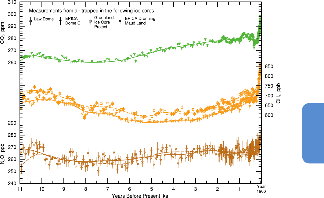
483
Carbon and Other Biogeochemical Cycles Chapter 6
6
in the atmospheric oxidising capacity of the atmosphere at the LGM
are probably negligible compared to changes in sources (Levine et al.,
2011) and that tropical temperature influencing tropical wetlands and
global vegetation were the dominant controls for CH
4
atmospheric
changes on glacial–interglacial time scales (Konijnendijk et al., 2011).
6.2.1.3 Processes Controlling Changes in Carbon Dioxide,
Methane, and Nitrous Oxide During Abrupt Glacial
Events
Ice core measurements of CO
2
, CH
4
and N
2
O show sharp (millen-
nial-scale) changes in the course of glaciations, associated with the
so-called Dansgaard/Oeschger (DO) climatic events (see Section 5.7),
but their amplitude, shape and timing differ. During these millennial
scale climate events, atmospheric CO
2
concentrations varied by about
20 ppm, in phase with Antarctic, but not with Greenland tempera-
tures. CO
2
increased during cold (stadial) periods in Greenland, several
thousands years before the time of the rapid warming event in Green-
land (Ahn and Brook, 2008). CH
4
and N
2
O showed rapid transitions in
phase with Greenland temperatures with little or no lag. CH
4
changes
are in the 50 to 200 ppb range (Flückiger et al., 2004), in phase with
Greenland temperature warming at a decadal time scale (Huber et al.,
2006). N
2
O changes are large, of same magnitude than glacial–inter-
glacial changes, and for the warmest and longest DO events N
2
O starts
to increase several centuries before Greenland temperature and CH
4
(Schilt et al., 2010b).
(
)
(
)
(
)
(
)
Figure 6.6 | Variations of CO
2
, CH
4
, and N
2
O concentrations during the Holocene. The data are for Antarctic ice cores: European Programme for Ice Coring in Antarctica EPICA
Dome C (Flückiger et al., 2002; Monnin et al., 2004), triangles; EPICA Dronning Maud Land (Schilt et al., 2010b), crosses; Law Dome (MacFarling-Meure et al., 2006), circles; and
for Greenland Ice Core Project (GRIP) (Blunier et al., 1995), squares. Lines correspond to spline fits.
Conflicting hypotheses exist on the drivers of these millennial-scale
changes. Some model simulations suggest that both CO
2
and N
2
O
fluctuations can be explained by changes in the Atlantic meridional
overturning ocean circulation (Schmittner and Galbraith, 2008), CO
2
variations being explained mainly by changes in the efficiency of the
biological pump which affects deep ocean carbon storage (Bouttes et
al., 2011), whereas N
2
O variations could be due to changes in produc-
tivity and oxygen concentrations in the subsurface ocean (Schmittner
and Galbraith, 2008). Other studies, however, suggest that the millen-
nial-scale CO
2
fluctuations can be explained by changes in the land
carbon storage (Menviel et al., 2008; Bozbiyik et al., 2011). For CH
4
,
models have difficulties in reproducing changes in wetland emissions
compatible with DO atmospheric variations (Hopcroft et al., 2011), and
the changes in the atmospheric oxidizing capacity of the atmosphere
during DO events seem to be too weak to explain the CH
4
changes
(Levine et al., 2012).
6.2.2 Greenhouse Gas Changes over the Holocene
6.2.2.1 Understanding Processes Underlying Holocene Carbon
Dioxide Changes
The evolution of the atmospheric CO
2
, CH
4
, and N
2
O concentrations
during the Holocene, the interglacial period which began 11.7 ka, is
known with high certainty from ice core measurements (Figure 6.6). A
decrease in atmospheric CO
2
of about 7 ppm is measured in ice cores

484
Chapter 6 Carbon and Other Biogeochemical Cycles
6
between 11 and 7 ka, followed by a 20 ppm CO
2
increase until the
onset of the Industrial Era in 1750 (Indermühle et al., 1999; Monnin et
al., 2004; Elsig et al., 2009). These variations in atmospheric CO
2
over
the past 11 kyr preceding industrialisation are more than five times
smaller than the CO
2
increase observed during the Industrial Era (see
Section 6.3.2.3). Despite the small magnitude of CO
2
variations prior
to the Industrial Era, these changes are nevertheless useful for under-
standing the role of natural forcing in carbon and other biogeochemi-
cal cycles during interglacial climate conditions.
Since the IPCC AR4, the mechanisms underlying the observed 20 ppm
CO
2
increase between 7 ka and the Industrial Era have been a matter
of intensive debate. During three interglacial periods prior to the Holo-
cene, CO
2
did not increase, and this led to a hypothesis that pre-indus-
trial anthropogenic CO
2
emissions could be associated with early land
use change and forest clearing (Ruddiman, 2003, 2007). However, ice
core CO
2
data (Siegenthaler et al., 2005b) indicate that during Marine
Isotope Stage 11 (see Section 5.2.2), an interglacial period that lasted
from 400 to 420 ka, CO
2
increased similarly to the Holocene period.
Drivers of atmospheric CO
2
changes during the Holocene can be divid-
ed into oceanic and terrestrial processes (Figure 6.5) and their roles are
examined below.
6.2.2.1.1 Oceanic processes
The change in oceanic carbonate chemistry could explain the slow
atmospheric CO
2
increase during the Holocene since 7 ka. Proposed
mechanisms include: (1) a shift of oceanic carbonate sedimentation
from deep sea to the shallow waters due to sea level rise onto con-
tinental shelves causing accumulation of CaCO
3
on shelves including
coral reef growth, a process that releases CO
2
to the atmosphere (Ridg-
well et al., 2003; Kleinen et al., 2010), (2) a ‘carbonate compensation’
in response to the release of carbon from the deep ocean during degla-
ciation and to the buildup of terrestrial biosphere in the early Holocene
(Broecker et al., 1999; Joos et al., 2004; Elsig et al., 2009; Menviel and
Joos, 2012). Proxies for carbonate ion concentration in the deep sea (Yu
et al., 2010) and a decrease in modern CaCO
3
preservation in equatori-
al Pacific sediments (Anderson et al., 2008) support the hypothesis that
the ocean was a source of CO
2
to the atmosphere during the Holocene.
Changes in SSTs over the last 7 kyr (Kim et al., 2004) could have con-
tributed to slightly lower (Brovkin et al., 2008) or higher (Menviel and
Joos, 2012) atmospheric CO
2
concentration but, very likely, SST-driven
CO
2
change represents only a minor contribution to the observed CO
2
increase during the Holocene after 7 ka (Figure 6.5).
6.2.2.1.2 Terrestrial processes
The δ
13
C of atmospheric CO
2
trapped in ice cores can be used to infer
changes in terrestrial biospheric carbon pools. Calculations based
on inferred δ
13
C of atmospheric CO
2
during the Holocene suggest
an increase in terrestrial carbon storage of about 300 PgC between
11 and 5 ka and small overall terrestrial changes thereafter (Elsig et
al., 2009). Modelling studies suggest that CO
2
fertilisation (Box 6.3)
in response to increasing atmospheric CO
2
concentration after 7 ka
contributed to a substantially increased terrestrial carbon storage
(>100 PgC) on Holocene time scales (Kaplan et al., 2002; Joos et al.,
2004; Kleinen et al., 2010). Orbitally forced climate variability, includ-
ing the intensification and decline of the Afro-Asian monsoon and the
mid-Holocene warming of the high latitudes of the NH are estimated
in models to have caused changes in vegetation distribution and hence
of terrestrial carbon storage. These climate-induced carbon storage
changes are estimated using models to have been smaller than the
increase due to CO
2
fertilisation (Brovkin et al., 2002; Schurgers et al.,
2006). The Holocene accumulation of carbon in peatlands has been
reconstructed globally, suggesting a land carbon additional storage of
several hundred petagrams of carbon between the early Holocene and
the Industrial Era, although uncertainties remain on this estimate (Tar-
nocai et al., 2009; Yu, 2011; Kleinen et al., 2012). Volcanic CO
2
emis-
sions to the atmosphere between 12 and 7 ka were estimated to be
two to six times higher than during the last millennium, of about 0.1
PgC yr
–1
(Huybers and Langmuir, 2009; Roth and Joos, 2012). However,
a peak in the inferred volcanic emissions coincides with the period of
decreasing atmospheric CO
2
and the confidence in changes of volcanic
CO
2
emissions is low.
Global syntheses of the observational, paleoecological and archaeolog-
ical records for Holocene land use change are not currently available
(Gaillard et al., 2010). Available reconstructions of anthropogenic land
use and land cover change (LULCC) prior to the last millennium cur-
rently extrapolate using models and assumptions from single regions
to changes in all regions of the world (Goldewijk et al., 2011; Kaplan
et al., 2011). Because of regional differences in land use systems and
uncertainty in historical population estimates, the confidence in spa-
tially explicit LULCC reconstructions is low.
Some recent studies focused on reconstructing LULCC and making very
simple assumptions regarding the effect of land use on carbon (Olofs-
son and Hickler, 2008; Lemmen, 2009). Other studies relied on more
sophisticated terrestrial biosphere models to simulate carbon storage
and loss in response to pre-industrial LULCC during the late Holocene
(Strassmann et al., 2008; Pongratz et al., 2009; Stocker et al., 2011).
The conclusion of the aforementioned studies was that cumulative
Holocene carbon emissions as a result of pre-industrial LULCC were
not large enough (~50 to 150 PgC during the Holocene before 1850)
to have had an influence larger than an increase of ~10 ppm on late
Holocene observed CO
2
concentration increase (Figure 6.5). However, a
modelling study by Kaplan et al. (2011) suggested that more than 350
PgC could have been released as a result of LULCC between 8 ka and
1850 as a result of a much stronger loss of soil carbon in response to
land use change, than in other studies.
In addition to clearing of forests, large-scale biomass burning activ-
ity, inferred from synthesized charcoal records and bog sediments
has been hypothesized to correlate with the observed Late Holocene
atmospheric CO
2
(Carcaillet et al., 2002). A global extensive synthesis
of charcoal records for the last 21 kyr (Power et al., 2008) and updates
of those shows that fire activity followed climate variability on global
(Marlon et al., 2008; Daniau et al., 2012) and regional scale (Archibald
et al., 2009; Mooney et al., 2011; Marlon et al., 2012; Power et al.,
2013). There is no evidence, however, for a distinct change in fire activ-
ity linked to human activity alone as hypothesized from a regional
charcoal record synthesis for the tropical Americas (Nevle and Bird,
2008; Nevle et al., 2011). Fire being a newly studied component, no
estimate for its role is given in Figure 6.5.
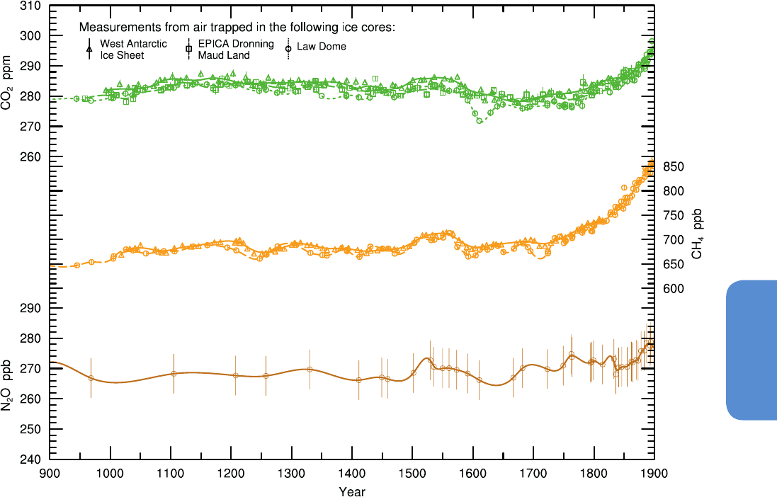
485
Carbon and Other Biogeochemical Cycles Chapter 6
6
6.2.2.2 Holocene Methane and Nitrous Oxide Drivers
The atmospheric CH
4
levels decreased from the early Holocene to about
6 ka, were lowest at around 5 ka, and increased between 5 ka and year
1750 by about 100 ppb (Figure 6.6). Major Holocene agricultural devel-
opments, in particular rice paddy cultivation and widespread domes-
tication of ruminants, have been proposed as an explanation for the
Late Holocene CH
4
rise (Ruddiman, 2007). The most recent syntheses
of archaeological data point to an increasing anthropogenic CH
4
source
from domesticated ruminants after 5 ka and from rice cultivation after 4
ka (Ruddiman, 2007; Fuller et al., 2011). The modelling support for either
natural or anthropogenic explanations of the Late Holocene increase in
the atmospheric CH
4
concentration is equivocal. A study by Kaplan et
al. (2006) suggested that a part of the Late Holocene CH
4
rise could
be explained by anthropogenic sources. Natural wetland CH
4
models
driven by simulated climate changes are able (Singarayer et al., 2011)
or unable (Konijnendijk et al., 2011) to simulate Late Holocene increase
in the CH
4
concentration, reflecting a large spread in present-day CH
4
emissions simulated by this type of models (Melton et al., 2013; see Sec-
tion 6.3.3.2). Consequently, about as likely as not, the atmospheric CH
4
increase after 5000 years ago can be attributed to early human activi-
ties. The mechanisms causing the N
2
O concentration changes during the
Holocene are not firmly identified (Flückiger et al., 2002).
(
)
(
)
(
)
Figure 6.7 | Variations of CO
2
, CH
4
, and N
2
O during 900–1900 from ice cores. The data are for Antarctic ice cores: Law Dome (Etheridge et al., 1996; MacFarling-Meure et al.,
2006), circles; West Antarctic Ice Sheet (Mitchell et al., 2011; Ahn et al., 2012), triangles; Dronning Maud Land (Siegenthaler et al., 2005a), squares. Lines are spline fits to individual
measurements.
6.2.3 Greenhouse Gas Changes over the Last Millennium
6.2.3.1 A Decrease of Carbon Dioxide around Year 1600 and
Possible Explanations for this Event
High resolution ice cores records reveal that atmospheric CO
2
during
the last millennium varied with a drop in atmospheric CO
2
concen-
tration by 7 to 10 ppm around year 1600, followed by a CO
2
increase
during the 17th century (Trudinger et al., 2002; Siegenthaler et al.,
2005a; MacFarling-Meure et al., 2006; Ahn et al., 2012). This is shown
in Figure 6.7. The CO
2
decrease during the 17th century was used to
evaluate the response of atmospheric CO
2
concentration to a centu-
ry-scale shift in global temperature (Scheffer et al., 2006; Cox and
Jones, 2008; Frank et al., 2010) which was found to be dependent on
the choice of global temperature reconstructions used in the model.
One of the possible explanations for the drop in atmospheric CO
2
around
year 1600 is enhanced land and/or ocean carbon uptake in response
to the cooling caused by reduced solar irradiance during the Maunder
Minimum (Section 5.3.5.3). However, simulations using Earth System
Models of Intermediate Complexity (EMICs)(Gerber et al., 2003; Brovkin
et al., 2004) and by complex Earth System Models (ESMs) (Jungclaus
et al., 2010) suggest that solar irradiance forcing alone is not sufficient

486
Chapter 6 Carbon and Other Biogeochemical Cycles
6
to explain the magnitude of the CO
2
decrease. The drop in atmospheric
CO
2
around year 1600 could also be caused by a cooling from increased
volcanic eruptions (Jones and Cox, 2001; Brovkin et al., 2010; Frölicher
et al., 2011). A third hypothesis calls for a link between CO
2
and epidem-
ics and wars associated with forest regrowth over abandoned lands and
increased carbon storage, especially in Central America. Here, results are
model and scenario dependent. Simulations by Pongratz et al. (2011a)
do not reproduce a decrease in CO
2
, while simulations by Kaplan et al.
(2011) suggest a considerable increase in land carbon storage around
year 1600. The temporal resolution of Central American charcoal and
pollen records is insufficient to support or falsify these model results
(e.g., Nevle and Bird, 2008; Marlon et al., 2008).
Ensemble simulations over the last 1200 years have been conducted
using an ESM (Jungclaus et al., 2010) and EMICs (Eby et al., 2013)
including a fully interactive carbon cycle. The sensitivity of atmospheric
CO
2
concentration to NH temperature changes in ESM was modeled to
be of 2.7 to 4.4 ppm °C
–1
, while EMICs show on average a higher sen-
sitivity of atmospheric CO
2
to global temperature changes of 8.6 ppm
°C
–1
.These sensitivities fall within the range of 1.7 to 21.4 ppm °C
–1
of
a recent reconstruction based on tree-ring NH temperature reconstruc-
tions (Frank et al., 2010).
6.2.3.2 Mechanisms Controlling Methane and Nitrous Oxide
during the Last Millennium
Recent high-resolution ice core records confirm a CH
4
decrease in the
late 16th century by about 40 ppb (MacFarling-Meure et al., 2006;
Mitchell et al., 2011), as shown in Figure 6.7. Correlations between this
drop in atmospheric CH
4
and the lower temperatures reconstructed
during the 15th and 16th centuries suggest that climate change may
have reduced CH
4
emissions by wetlands during this period. In addition
1750–2011
Cumulative
PgC
1980–1989
PgC yr
–1
1990–1999
PgC yr
–1
2000–2009
PgC yr
–1
2002–2011
PgC yr
–1
Atmospheric increase
a
240 ± 10
f
3.4 ± 0.2 3.1 ± 0.2 4.0 ± 0.2 4.3 ± 0.2
Fossil fuel combustion and cement production
b
375 ± 30
f
5.5 ± 0.4 6.4 ± 0.5 7.8 ± 0.6 8.3 ± 0.7
Ocean-to-atmosphere flux
c
–155 ± 30
f
–2.0 ± 0.7 –2.2 ± 0.7 –2.3 ± 0.7 –2.4 ± 0.7
Land-to-atmosphere flux
Partitioned as follows
30 ± 45
f
–0.1 ± 0.8 –1.1 ± 0.9 –1.5 ± 0.9 –1.6 ± 1.0
Net land use change
d
180 ± 80
f,g
1.4 ± 0.8 1.5 ± 0.8 1.1 ± 0.8 0.9 ± 0.8
Residual land sink
e
–160 ± 90
f
–1.5 ± 1.1 –2.6 ± 1.2 –2.6 ± 1.2 –2.5 ± 1.3
Table 6.1 | Global anthropogenic CO
2
budget, accumulated since the Industrial Revolution (onset in 1750) and averaged over the 1980s, 1990s, 2000s, as well as the last 10 years
until 2011. By convention, a negative ocean or land to atmosphere CO
2
flux is equivalent to a gain of carbon by these reservoirs. The table does not include natural exchanges (e.g.,
rivers, weathering) between reservoirs. The uncertainty range of 90% confidence interval presented here differs from how uncertainties were reported in AR4 (68%).
to changes in the wetland CH
4
source, changes in biomass burning have
been invoked to explain the last millennium CH
4
record (Ferretti et al.,
2005; Mischler et al., 2009), ice core CO and CO isotopes (Wang et al.,
2010b) and global charcoal depositions (Marlon et al., 2008). Chang-
es in anthropogenic CH
4
emissions during times of war and plague
hypothetically contributed to variability in atmospheric CH
4
concentra-
tion (Mitchell et al., 2011). Ice core δ
13
CH
4
measurements suggested
pronounced variability in both natural and anthropogenic CH
4
sources
over the 1000–1800 period (Sapart et al., 2012). No studies are known
about mechanisms of N
2
O changes for the last millennium.
6.3 Evolution of Biogeochemical Cycles
Since the Industrial Revolution
6.3.1 Carbon Dioxide Emissions and Their Fate
Since 1750
Prior to the Industrial Era, that began in 1750, the concentration of
atmospheric CO
2
fluctuated roughly between 180 ppm and 290 ppm
for at least 2.1 Myr (see Section 5.2.2 and Hönisch et al., 2009; Lüthi
et al., 2008; Petit et al., 1999). Between 1750 and 2011, the combus-
tion of fossil fuels (coal, gas, oil and gas flaring) and the production of
cement have released 375 ± 30 PgC (1 PgC = 10
15
gC) to the atmos-
phere (Table 6. 1; Boden et al., 2011). Land use change activities, mainly
deforestation, has released an additional 180 ± 80 PgC (Table 6.1). This
carbon released by human activities is called anthropogenic carbon.
Of the 555 ± 85 PgC of anthropogenic carbon emitted to the atmos-
phere from fossil fuel and cement and land use change, less than half
have accumulated in the atmosphere (240 ± 10 PgC) (Table 6.1). The
remaining anthropogenic carbon has been absorbed by the ocean and
Notes:
a
Data from Charles D. Keeling, (http://scrippsco2.ucsd.edu/data/data.html), Thomas Conway and Pieter Tans, National Oceanic and Atmospheric Administration–Earth System Research Laboratory
(NOAA–ESRL, www.esrl.noaa.gov/gmd/ccgg/trends/) using a conversion factor of 2.120 PgC per ppm (Prather et al., 2012). Prior to the atmospheric record in 1960, ice core data is used (Neftel
et al., 1982; Friedli et al., 1986; Etheridge et al., 1996).
b
Estimated by the Carbon Dioxide Information Analysis Center (CDIAC) based on UN energy statistics for fossil fuel combustion (up to 2009) and US Geological Survey for cement production
(Boden et al., 2011), and updated to 2011 using BP energy statistics.
c
Based on observations for 1990–1999, with the trends based on existing global estimates (see Section 6.3.2.5 and Table 6.4).
d
Based on the “bookkeeping” land use change flux accounting model of Houghton et al. (2012) until 2010, and assuming constant LUC emissions for 2011, consistent with satellite-based fire
emissions (Le Quéré et al., 2013; see Section 6.3.2.2 and Table 6.2).
e
Calculated as the sum of the Land-to-atmosphere flux minus Net land use change flux, assuming the errors on each term are independent and added quadratically.
f
The 1750–2011 estimate and its uncertainty is rounded to the nearest 5 PgC.
g
Estimated from the cumulative net land use change emissions of Houghton et al. (2012) during 1850–2011 and the average of four publications (Pongratz at al., 2009; van Minnen et al., 2009;
Shevliakova et al., 2009; Zaehle et al., 2011) during 1750–1850.
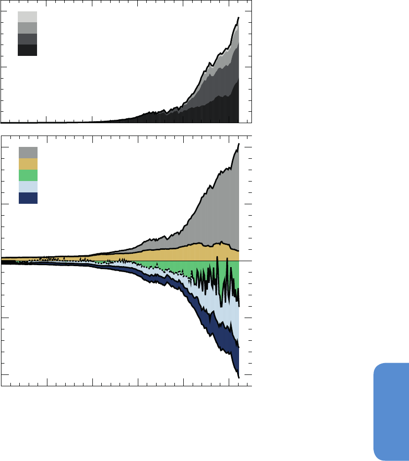
487
Carbon and Other Biogeochemical Cycles Chapter 6
6
in terrestrial ecosystems: the carbon ‘sinks’ (Figure 6.8). The ocean
stored 155 ± 30 PgC of anthropogenic carbon since 1750 (see Sec-
tion 6.3.2.5.3 and Box 6.1). Terrestrial ecosystems that have not been
affected by land use change since 1750, have accumulated 160 ± 90
PgC of anthropogenic carbon since 1750 (Table 6.1), thus not fully
compensating the net CO
2
losses from terrestrial ecosystems to the
atmosphere from land use change during the same period estimated
of 180 ± 80 PgC (Table 6.1). The net balance of all terrestrial ecosys-
Figure 6.8 | Annual anthropogenic CO
2
emissions and their partitioning among the atmosphere, land and ocean (PgC yr
–1
) from 1750 to 2011. (Top) Fossil fuel and cement CO
2
emissions by category, estimated by the Carbon Dioxide Information Analysis Center (CDIAC) based on UN energy statistics for fossil fuel combustion and US Geological Survey
for cement production (Boden et al., 2011). (Bottom) Fossil fuel and cement CO
2
emissions as above. CO
2
emissions from net land use change, mainly deforestation, are based
on land cover change data and estimated for 1750–1850 from the average of four models (Pongratz et al., 2009; Shevliakova et al., 2009; van Minnen et al., 2009; Zaehle et
al., 2011) before 1850 and from Houghton et al. (2012) after 1850 (see Table 6.2). The atmospheric CO
2
growth rate (term in light blue ‘atmosphere from measurements’ in the
figure) prior to 1959 is based on a spline fit to ice core observations (Neftel et al., 1982; Friedli et al., 1986; Etheridge et al., 1996) and a synthesis of atmospheric measurements
from 1959 (Ballantyne et al., 2012). The fit to ice core observations does not capture the large interannual variability in atmospheric CO
2
and is represented with a dashed line.
The ocean CO
2
sink prior to 1959 (term in dark blue ‘ocean from indirect observations and models’ in the figure) is from Khatiwala et al. (2009) and from a combination of models
and observations from 1959 from (Le Quéré et al., 2013). The residual land sink (term in green in the figure) is computed from the residual of the other terms, and represents
the sink of anthropogenic CO
2
in natural land ecosystems. The emissions and their partitioning only include the fluxes that have changed since 1750, and not the natural CO
2
fluxes (e.g., atmospheric CO
2
uptake from weathering, outgassing of CO
2
from lakes and rivers, and outgassing of CO
2
by the ocean from carbon delivered by rivers; see Figure
6.1) between the atmosphere, land and ocean reservoirs that existed before that time and still exist today. The uncertainties in the various terms are discussed in the text and
reported in Table 6.1 for decadal mean values.
cement
gas
oil
coal
fossil fuel and cement from energy statistics
land use change from data and models
residual land sink
measured atmospheric growth rate
ocean sink from data and models
1750 1800 1850 1900 1950 2000
10
5
5
10
0
5
10
0
1750 1800 1850 1900 1950 2000
emissions
partitioning
Annual anthropogenic CO
2
emissions
and partitioning (PgC yr
–1
)
Fossil fuel and cement
CO
2
emissions (PgC yr
–1
)
Year
tems, those affected by land use change and the others, is thus close
to neutral since 1750, with an average loss of 30 ± 45 (see Figure 6.1).
This increased storage in terrestrial ecosystems not affected by land
use change is likely to be caused by enhanced photosynthesis at higher
CO
2
levels and nitrogen deposition, and changes in climate favouring
carbon sinks such as longer growing seasons in mid-to-high latitudes.
Forest area expansion and increased biomass density of forests that
result from changes in land use change are also carbon sinks, and they
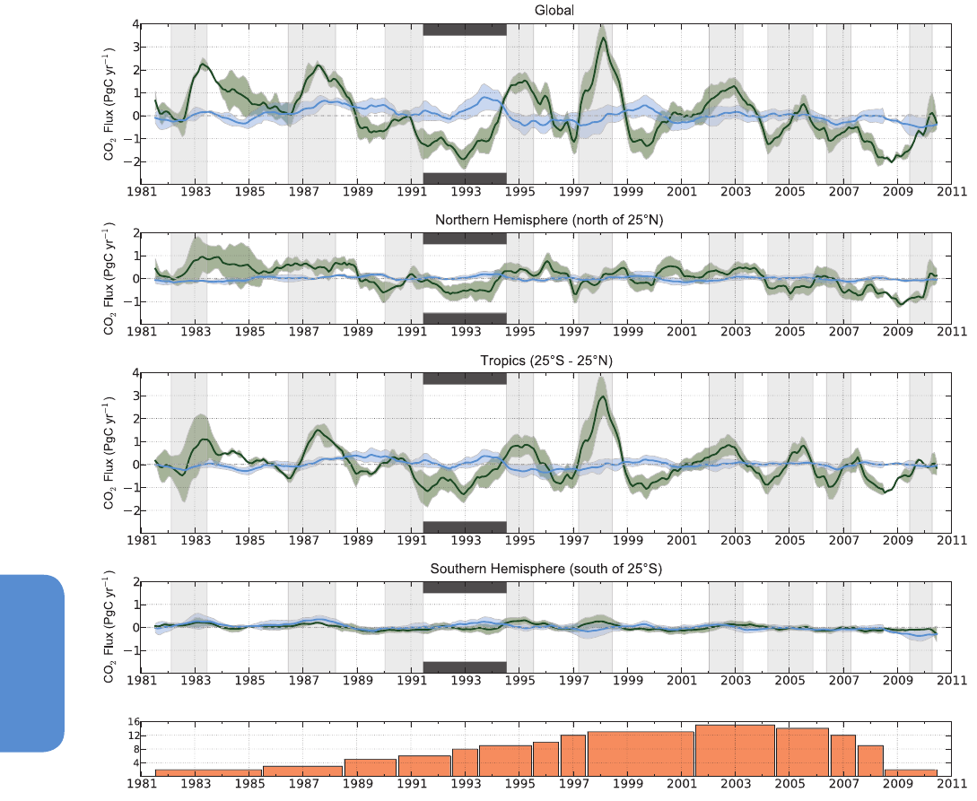
488
Chapter 6 Carbon and Other Biogeochemical Cycles
6
are accounted in Table 6.1 as part of the net flux from land use change.
The increased terrestrial carbon storage in ecosystems not affected by
land use change is called the Residual land sink in Table 6.1 because
it is inferred from mass balance as the difference between fossil and
net land use change emissions and measured atmospheric and oceanic
storage increase.
6.3.2 Global Carbon Dioxide Budget
Since the IPCC AR4 (Denman et al., 2007), a number of new advance-
ments in data availability and data-model synthesis have allowed the
establishment of a more constrained anthropogenic CO
2
budget and
better attribution of its flux components. The advancements are: (1)
Number of inversion models
Figure 6.9 | Interannual surface CO
2
flux anomalies from inversions of the TRANSCOM project for the period 1981–2010 (Peylin et al., 2013). The ensemble of inversion results
contains up to 17 atmospheric inversion models. The orange bars in the bottom panel indicate the number of available inversion models for each time period. The ensemble mean
is bounded by the 1-σ inter-model spread in ocean–atmosphere (blue) and land–atmosphere (green) CO
2
fluxes (PgC yr
–1
) grouped into large latitude bands, and the global. For
each flux and each region, the CO
2
flux anomalies were obtained by subtracting the long-term mean flux from each inversion and removing the seasonal signal. Grey shaded regions
indicate El Niño episodes, and the black bars indicate the cooling period following the Mt. Pinatubo eruption, during which the growth rate of CO
2
remained low. A positive flux
means a larger than normal source of CO
2
to the atmosphere (or a smaller CO
2
sink).
revised data on the rates of land use change conversion from country
statistics (FAO, 2010) now providing an arguably more robust estimate
of the land use change flux (Houghton et al., 2012; Section 6.3.2.2);
(2) a new global compilation of forest inventory data that provides an
independent estimate of the amount of carbon that has been gained
by forests over the past two decades, albeit with very scarce measure-
ments for tropical forest (Pan et al., 2011); (3) over 2 million new obser-
vations of the partial pressure of CO
2
(pCO
2
) at the ocean surface have
been taken and added to the global databases (Takahashi et al., 2009;
Pfeil et al., 2013) and used to quantify ocean CO
2
sink variability and
trends (Section 6.3.2.5) and to evaluate and constrain models (Schuster
et al., 2013; Wanninkhof et al., 2013); and (4) the use of multiple con-
straints with atmospheric inversions and combined atmosphere–ocean

489
Carbon and Other Biogeochemical Cycles Chapter 6
6
inversions (so called top down approaches; Jacobson et al., 2007) and
the up-scaling of reservoir-based observations using models (so called
bottom up approaches) provides new coarse scale consistency checks
on CO
2
flux estimates for land and ocean regions (McGuire et al., 2009;
Piao et al., 2009b; Schulze et al., 2009; Ciais et al., 2010; Schuster et al.,
2013). The causes of the year-to-year variability observed in the annual
atmospheric CO
2
accumulation shown in Figure 6.8 are estimated with
a medium to high confidence to be mainly driven by terrestrial pro-
cesses occurring in tropical latitudes as inferred from atmospheric CO
2
inversions and supported by ocean data and models (Bousquet et al.,
2000; Raupach et al., 2008; Sarmiento et al., 2010) (Figures 6.9 and
6.13; Section 6.3.2.5) and land models (Figure 6.16; Section 6.3.2.6).
6.3.2.1 Carbon Dioxide Emissions from Fossil Fuel Combustion
and Cement Production
Global CO
2
emissions from the combustion of fossil fuels used for this
chapter are determined from national energy consumption statistics
and converted to emissions by fuel type (Marland and Rotty, 1984).
Estimated uncertainty for the annual global emissions are on the order
of ±8% (converted from ±10% uncertainty for 95% confidence inter-
vals in Andres et al. (2012) to the 90% confidence intervals used here).
The uncertainty has been increasing in recent decades because a larger
fraction of the global emissions originate from emerging economies
where energy statistics and emission factors per fuel type are more
uncertain (Gregg et al., 2008). CO
2
emissions from cement production
were 4% of the total emissions during 2000–2009, compared to 3% in
the 1990s (Boden et al., 2011). Additional emissions from gas flaring
represent <1% of the global emissions.
Global CO
2
emissions from fossil fuel combustion and cement produc-
tion were 7.8 ± 0.6 PgC yr
–1
on average during 2000–2009, 6.4 ± 0.5
PgC yr
–1
during 1990–1999 and 5.5 ± 0.4 PgC yr
–1
during 1980–1989
(Table 6.1; Figure 6.8). Global fossil fuel CO
2
emissions increased by
3.2% yr
–1
on average during the decade 2000–2009 compared to
1.0% yr
–1
in the 1990s and 1.9% yr
–1
in the 1980s. Francey et al. (2013)
recently suggested a cumulative underestimation of 8.8 PgC emissions
during the period 1993–2004, which would reduce the contrast in
emissions growth rates between the two decades. The global financial
crisis in 2008–2009 induced only a short-lived drop in global emis-
sions in 2009 (–0.3%), with the return to high annual growth rates
of 5.1% and 3.0% in 2010 and 2011, respectively, and fossil fuel and
cement CO
2
emissions of 9.2 ± 0.8 PgC in 2010 and 9.5 ± 0.8 PgC in
2011(Peters et al., 2013).
6.3.2.2 Net Land Use Change Carbon Dioxide Flux
CO
2
is emitted to the atmosphere by land use and land use change
activities, in particular deforestation, and taken up from the atmos-
phere by other land uses such as afforestation (the deliberate creation
of new forests) and vegetation regrowth on abandoned lands. A critical
distinction in estimating land use change is the existence of gross and
net fluxes. Gross fluxes are the individual fluxes from multiple pro-
cesses involved in land use change that can be either emissions to
or removals from the atmosphere occurring at different time scales.
For example, gross emissions include instantaneous emissions from
deforestation fires and long-term emissions from the decomposition
of organic carbon; and they also include the long-term CO
2
uptake by
forest regrowth and soil carbon storage on abandoned agricultural
lands, afforestation and storage changes of wood products (Houghton
et al., 2012; Mason Earles et al., 2012). The net flux of land use change
is the balance among all source and sink processes involved in a given
timeframe. The net flux of land use change is globally a net source to
the atmosphere (Table 6.1; Figure 6.8).
Approaches to estimate global net CO
2
fluxes from land use fall into
three categories: (1) the ‘bookkeeping’ method that tracks carbon in
living vegetation, dead plant material, wood products and soils with
cultivation, harvesting and reforestation using country-level reports on
changes in forest area and biome-averaged biomass values (Houghton,
2003); (2) process-based terrestrial ecosystem models that simulate
on a grid-basis the carbon stocks (biomass, soils) and exchange fluxes
between vegetation, soil and atmosphere (see references in Table 6.2)
and (3) detailed regional (primarily tropical forests) analyses based on
satellite data that estimate changes in forest area or biomass (DeFries
et al., 2002; Achard et al., 2004; Baccini et al., 2012; Harris et al., 2012).
Satellite-derived estimates of CO
2
emissions to the atmosphere from
so-called deforestation fires (van der Werf et al., 2010) provide addi-
tional constraints on the spatial attribution and variability of land use
change gross emissions. Most global estimates do not include emis-
sions from peat burning or decomposition after a land use change,
which are estimated to be 0.12 PgC yr
–1
over 1997–2006 for peat fires
(van der Werf et al., 2008) and between 0.10 and 0.23 PgC yr
–1
from
the decomposition of drained peat (Hooijer et al., 2010). The processes
and time scales captured by these methods to estimate net land use
change CO
2
emissions are diverse, creating difficulties with comparison
of different estimates (Houghton et al., 2012; Table 6.2). The bookkeep-
ing method of Houghton et al. (2012) was used for Table 6.1 because it
is closest to observations and includes the most extensive set of man-
agement practices (Table 6.2). Methods that do not include long-term
‘legacy’ fluxes from soils caused by deforestation (Table 6.2) underes-
timate net land use change CO
2
emissions by 13 to 62% depending on
the starting year and decade (Ramankutty et al., 2006), and methods
that do not include the fate of carbon wood harvest and shifting cul-
tivation underestimate CO
2
emissions by 25 to 35% (Houghton et al.,
2012).
Global net CO
2
emissions from land use change are estimated at 1.4,
1.5 and 1.1 PgC yr
–1
for the 1980s, 1990s and 2000s, respectively, by
the bookkeeping method of Houghton et al. (2012) (Table 6.2; Figure
6.10). This estimate is consistent with global emissions simulated by
process-based terrestrial ecosystem models using mainly three land
cover change data products as input for time-varying maps of land use
change (Table 6.2). The bookkeeping method estimate is also generally
consistent although higher than the satellite-based methods (tropics
only). Part of the discrepancy can be accounted for by emissions from
extratropical regions (~0.1 PgC yr
–1
; Table 6.3) and by legacy fluxes for
land cover change prior to 1980s (~0.2 PgC yr
–1
) that are not covered
by satellite-based methods used in Table 6.2, and by the fact that the
bookkeeping method accounts for degradation and shifting agriculture
CO
2
losses not detected in the satellite-based method reported in Table
6.2. We adopt an uncertainty of ±0.8 PgC yr
–1
as representative of
90% uncertainty intervals. This is identical to the uncertainty of ±0.5
PgC yr
–1
representing ±1-σ interval (68% if Gaussian distributed error)

490
Chapter 6 Carbon and Other Biogeochemical Cycles
6
Data for
Land Use
Change Area
a
Biomass
Data
Land
Management
Included
Processes
Included
1980–1989
PgC yr
–1
1990–1999
PgC yr
–1
2000–2009
PgC yr
–1
Bookkeeping Method (global)
Houghton et al. (2012) FAO-2010 Observed
b
W, C, H I, D, R, S, L 1.4 1.5 1.1
Baccini et al. (2012) FAO-2010 Satellite data W, C, H I, D, R, S, L 1.0
Satellite-based Methods (tropics only)
Achard et al. (2004) Landsat Observed
b
I, D, R, S, C, M 0.9 (0.5–1.4)
c
DeFries et al. (2002) AVHRR Observed
b
I, D, R, S
d
, C, M 0.6 (0.3–0.8) 0.9 (0.5–1.4)
Van der Werf et al. (2010) GFED CASA
e
P I, D, C, M 1.2 (0.6–1.8)
f
Process Models (global)
Shevliakova et al. (2009) HYDE LM3V W, C I, D, R, S, L, C 1.1 1.1
Shevliakova et al. (2009) SAGE LM3V W, C I, D, R, S, L, C 1.4 1.3
van Minnen et al. (2009)
g
HYDE IMAGE 2
e
W I, D, R, S, L, C 1.8 1.4 1.2
Strassmann et al. (2008) HYDE BernCC
e
I, D, R, S, L, C 1.3 1.3
Stocker et al. (2011)
g
HYDE BernCC
e
H I, D, R, S, L, C 1.4 0.9 0.6
Yang et al. (2010) SAGE ISAM
e
W I, D, R, S, L, C 1.7 1.7
Yang et al. (2010) FAO-2005 ISAM
e
W I, D, R, S, L, C 1.7 1.8
Yang et al. (2010)
g
HYDE ISAM
e
W I, D, R, S, L, C 2.2 1.5 1.2
Arora and Boer (2010) SAGE CTEM
e
H I, D, R, S, L, C 1.1
h
1.1
h
Arora and Boer (2010)
g
HYDE CTEM
e
H I, D, R, S, L, C 0.4
h
0.4
h
Poulter et al. (2010)
g
HYDE LPJmL
e
I, D, R, S, L, C 1.0 0.9 0.5
Kato et al. (2013)
g
HYDE VISIT
e
C I, D, R, S, L, C 1.2 1.0 0.5
Zaehle et al. (2011) HYDE O-CN I, D, R, S, L, C 1.2 1.0
Average of process models
i
1.3 ± 0.7 1.2 ± 0.6 0.8 ± 0.6
Range of process models [0.4–2.2] [0.4–1.8] [0.5–1.2]
Table 6.2 | Estimates of net land to atmosphere CO
2
flux from land use change covering recent decades (PgC yr
–1
). Positive values indicate CO
2
losses to the atmosphere. Vari-
ous forms of land management are also included in the different estimates, including wood harvest (W), shifting cultivation (C) and harvesting (H) of crops and peat burning and
peat drainage (P). All methods include the vegetation degradation after land clearance. Additional processes included are initial biomass loss during the year of deforestation (I),
decomposition of slash and soil carbon during the year of initial loss (D), regrowth (R), change in storage in wood products pools (S), the effect of increasing CO
2
, (C), the effect
of observed climate variability between decades (M) and ‘legacy’ long-term decomposition flux carried over from land use change transitions prior to start of time period used for
reporting in the table (L). In the absence of data on L in the assessed estimates, the studies have either assumed instantaneous loss of all biomass and soil carbon (I, a committed
future flux) or did not consider the legacy flux L. Satellite-based methods have examined Land Use Change (LUC) emissions in the tropical regions only. Numbers in parentheses
are ranges in uncertainty provided in some studies.
Notes:
a
References for the databases used: FAO (2010) as applied in Houghton et al. (2012); FAO (2005) as applied in Houghton (2003), updated; GFED (van der Werf et al., 2009); HYDE (Goldewijk et
al., 2011), SAGE (Ramankutty and Foley, 1999). Landsat and AVHRR are satellite-based data and GFED is derived from satellite products as described in the references.
b
Based on average estimates by biomes compiled from literature data (see details in corresponding references).
c
1990–1997 only.
d
Legacy fluxes for land cover change prior to 1980 are not included and are estimated to add about 0.2 PgC yr
–1
to the 1980s and 0.1 PgC yr
–1
to the 1990s estimates, based on Ramankutty et
al. (2006).
e
The vegetation and soil biomass is computed using a vegetation model described in the reference.
f
1997–2006 average based on estimates of carbon emissions from deforestation and degradation fires, including peat fires and oxidation. Estimates were doubled to account for emissions other
than fire including respiration of leftover plant materials and soil carbon following deforestation following (Olivier et al., 2005).
g
Method as described in the reference but updated to 2010 using the land cover change data listed in column 2.
h
The large variability produced by the calculation method is removed for comparison with other studies by averaging the flux over the two decades.
i
Average of estimates from all process models and 90% confidence uncertainty interval; note that the spread of the different estimates does not follow a Gaussian distribution.
AVHRR = Advanced Very High Resolution Radiometer; FAO = Food and Agriculture Organization (UN); GFED = Global Fire Emissions Database; HYDE = HistorY Database of the global Environ-
ment; SAGE = Center for Sustainability and the Global Environment.
from Houghton et al. (2012). This uncertainty of ±0.8 PgC yr
–1
on net
land use change CO
2
fluxes is smaller than the one that was reported
in AR4 of 0.5 to 2.7 PgC yr
–1
for the 1990s (68% confidence interval). In
this chapter, uncertainty is estimated based on expert judgment of the
available evidence, including improved accuracy of land cover change
incorporating satellite data, the larger number of independent meth-
ods to quantify emissions and the consistency of the reported results
(Table 6.2; Figure 6.10).
Different estimates of net land use change CO
2
emissions are shown in
Figure 6.10. The lower net land use change CO
2
emissions reported in
the 2000s compared to the 1990s, by 0.5 PgC yr
–1
in the bookkeeping
method based on FAO (2010), and by 0.3 to 0.5 PgC yr
–1
from five
process-based ecosystem models based on the HistorY Database of the
global Environment (HYDE) land cover change data updated to 2009
(Goldewijk et al., 2011), are within the error bar of the data and meth-
ods. The bookkeeping method suggests that most of the LUC emissions
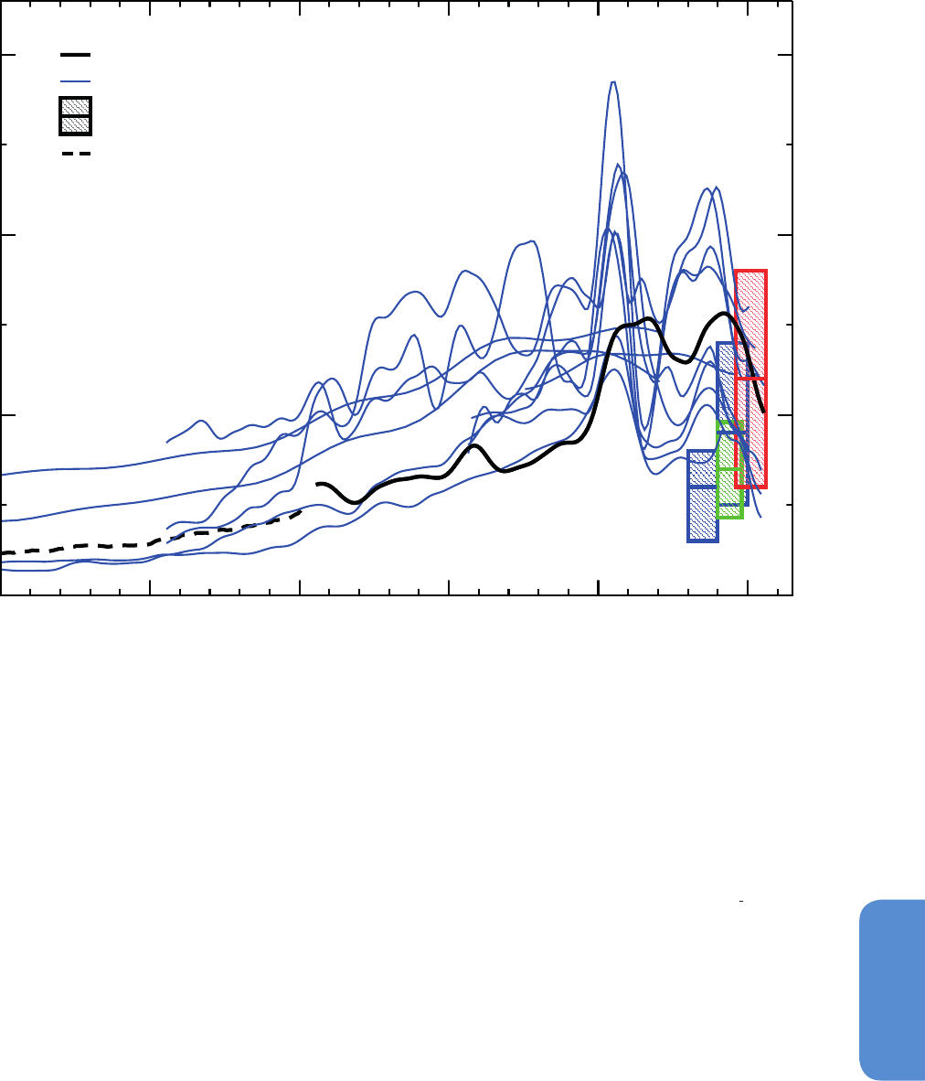
491
Carbon and Other Biogeochemical Cycles Chapter 6
6
Figure 6.10 | Net land use change CO
2
emissions (PgC yr
–1
). All methods are based on land cover change data (see Table 6.2) and are smoothed with a 10-year filter to remove
interannual variability. The bookkeeping estimate of Houghton et al. (2012) (thick black over 1850–2011) and the average of four process models (dash black) over 1750–1850
(see 6.3.2.2) are used in Table 6.1. The process model results for net land use change CO
2
emissions from Table 6.2 are shown in blue. Satellite-based methods are available for
the tropics only, from (red) van der Werf et al. (2010), (blue) DeFries et al. (2002), and (green) Achard et al. (2004). Note that the definitions of land use change fluxes vary between
models (Table 6.2). The grey shading shows a constant uncertainty of ±0.8 PgC yr
-1
around the mean estimate used in Table 6.3.
Houghton et al. (2012)
Process models (Table 6.2)
Satellite-based methods (see legend)
Average of four models (see Secton 6.3.2.2)
3
2
1
0
1750 1800
1850 1900 1950 2000
Net Land Use Change CO
2
emissions (PgC yr
-1
)
originate from Central and South America, Africa and Tropical Asia
since the 1980s (Table 6.3). The process models based on the HYDE
database allocate about 30% of the global land use change emissions
to East Asia, but this is difficult to reconcile with the large afforestation
programmes reported in this region. Inconsistencies in the available
land cover change reconstructions and in the modelling results pre-
vent a firm assessment of recent trends and their partitioning among
regions (see regional data in Table 6.3).
In this chapter, we do not assess individual gross fluxes that sum up
to make the net land use change CO
2
emission, because there are too
few independent studies. Gross emissions from tropical deforestation
and degradation were 3.0 ± 0.5 PgC yr
–1
for the 1990s and 2.8 ± 0.5
PgC yr
–1
for the 2000s using forest inventory data, FAO (2010) and the
bookeeping method (Pan et al., 2011). These gross emissions are about
double the net emissions because of the presence of a large regrowth
that compensates for about half of the gross emissions. A recent anal-
ysis estimated a lower gross deforestation of 0.6 to 1.2 PgC yr
–1
(Harris
et al., 2012). That study primarily estimated permanent deforestation
and excluded additional gross emissions from degraded forests, shift-
ing agriculture and some carbon pools. In fact, gross emissions from
permanent deforestation are in agreement between the bookkeeping
method of Houghton et al. (2012) and the satellite data analysis of
Harris et al. (2012).
Over the 1750–2011 period, cumulative net CO
2
emissions from land
use change of 180 ± 80 PgC are estimated (Table 6.1). The uncertainty
is based on the spread of the available estimates (Figure 6.10). The
cumulative net CO
2
emissions from land use change have been domi-
nated by deforestation and other land use change in the mid-northern
latitudes prior to 1980s, and in the tropics since the 1980s, largely from
deforestation in tropical America and Asia with smaller contributions
from tropical Africa. Deforestation from 800 to 1750 has been estimat-
ed at 27 PgC using a process-based ecosystem model (Pongratz et al.,
2009).
6.3.2.3 Atmospheric Carbon Dioxide Concentration Growth Rate
Since the beginning of the Industrial Era (1750), the concentration of
CO
2
in the atmosphere has increased by 40%, from 278 ± 5 ppm to
390.5 ± 0.1 ppm in 2011 (Figure 6.11; updated from Ballantyne et al.
(2012), corresponding to an increase in CO
2
of 240 ± 10 PgC in the

492
Chapter 6 Carbon and Other Biogeochemical Cycles
6
Table 6.3 | Estimates of net land to atmosphere flux from land use change (PgC yr
–1
; except where noted) for decadal periods from 1980s to 2000s by region. Positive values
indicate net CO
2
losses from land ecosystems affected by land use change to the atmosphere. Uncertainties are reported as 90% confidence interval (unlike 68% in AR4). Numbers
in parentheses are ranges in uncertainty provided in some studies. Tropical Asia includes the Middle East, India and surrounding countries, Indonesia and Papua New Guinea. East
Asia includes China, Japan, Mongolia and Korea.
Land Cover
Data
Central and
South Americas
Africa
Tropical
Asia
North
America
Eurasia East Asia Oceania
2000s
van der Werf et al. (2010)
a,b
GFED 0.33 0.15 0.35
DeFries and Rosenzweig (2010)
c
MODIS 0.46 0.08 0.36
Houghton et al. (2012) FAO-2010 0.48 0.31
e
0.25 0.01 –0.07
d
0.01
e
van Minnen et al. (2009)
a
HYDE 0.45 0.21 0.20 0.09 0.08 0.10 0.03
Stocker et al. (2011)
a
HYDE 0.19 0.18 0.21 0.019 –0.067 0.12 0.011
Yang et al. (2010)
a
HYDE 0.14 0.03 0.25 0.25 0.39 0.12 0.02
Poulter et al. (2010)
a
HYDE 0.09 0.13 0.14 0.01 0.03 0.05 0.00
Kato et al. (2013)
a
HYDE 0.36 –0.09 0.23 –0.05 –0.04 0.10 0.00
Average 0.31 ± 0.25 0.13 ± 0.20 0.25 ± 0.12 0.05 ± 0.17 0.12 ± 0.31 0.08 ± 0.07 0.01 ± 0.02
1990s
DeFries et al. (2002) AVHRR 0.5
(0.2–0.7)
0.1
(0.1–0.2)
0.4
(0.2–0.6)
Achard et al. (2004) Landsat 0.3
(0.3–0.4)
0.2
(0.1–0.2)
0.4
(0.3–0.5)
Houghton et al. (2012) FAO-2010 0.67 0.32
e
0.45 0.05 –0.04
d
0.05
e
van Minnen et al. (2009)
a
HYDE 0.48 0.22 0.34 0.07 0.08 0.20 0.07
Stocker et al. (2011)
a
HYDE 0.30 0.14 0.19 –0.072 0.11 0.27 0.002
Yang et al. (2010)
a
HYDE 0.20 0.04 0.31 0.27 0.47 0.19 0.00
Poulter et al. (2010)
a
HYDE 0.26 0.13 0.12 0.07 0.16 0.11 0.01
Kato et al. (2013)
a
HYDE 0.53 0.07 0.25 –0.04 –0.01 0.16 0.02
Average 0.41 ± 0.27 0.15 ± 0.15 0.31 ± 0.19 0.08 ± 0.19 0.16 ± 0.30 0.16 ± 0.13 0.02 ± 0.05
1980s
DeFries et al. (2002) AVHRR 0.4
(0.2–0.5)
0.1
(0.08–0.14)
0.2
(01–0.3)
Houghton et al. (2012) FAO-2010 0.79 0.22
e
0.32 0.04 0.00
d
0.07
e
van Minnen et al. (2009)
a
HYDE 0.70 0.18 0.43 0.07 0.06 0.37 0.04
Stocker et al. (2011)
a
HYDE 0.44 0.16 0.25 0.085 0.11 0.40 0.009
Yang et al. (2010)
a
HYDE 0.26 0.01 0.34 0.30 0.71 0.59 0.00
Poulter et al. (2010)
a
HYDE 0.37 0.11 0.19 0.02 0.03 0.29 0.01
Kato et al. (2013)
a
HYDE 0.61 0.07 0.25 –0.04 –0.02 0.35 0.01
Average 0.51 ± 0.32 0.12 ± 0.12 0.28 ± 0.14 0.08 ± 0.19 0.15 ± 0.46 0.35 ± 0.28 0.01 ± 0.03
Notes:
a
Method as described in the reference but updated to 2010 using the HYDE land cover change data.
b
1997–2006 average based on estimates of CO
2
emissions from deforestation and degradation fires, including peat carbon emissions. Estimates were doubled to account for emissions other than
fire including respiration of leftover plant materials and soil carbon following deforestation following (Olivier et al., 2005). Estimates include peat fires and peat soil oxidation. If peat fires are
excluded, estimate in tropical Asia is 0.23 and Pan-tropical total is 0.71.
c
CO
2
estimates were summed for dry and humid tropical forests, converted to C and normalized to annual values. Estimates are based on satellite-derived deforestation area (Hansen et al., 2010),
and assume 0.6 fraction of biomass emitted with deforestation. Estimates do not include carbon uptake by regrowth or legacy fluxes from historical deforestation. Estimates cover emissions
from 2000 to 2005.
d
Includes China only.
e
East Asia and Oceania are averaged in one region. The flux is split in two equally for computing the average; North Africa and the Middle East are combined with Eurasia.
AVHRR = Advanced Very High Resolution Radiometer; FAO = Food and Agriculture Organization (UN); GFED = Global Fire Emissions Database; HYDE = HistorY Database of the global Environ-
ment; MODIS = Moderate Resolution Imaging Spectrometer.
atmosphere. Atmospheric CO
2
grew at a rate of 3.4 ± 0.2 PgC yr
–1
in
the 1980s, 3.1 ± 0.2 PgC yr
–1
in the 1990s and 4.0 ± 0.2 PgC yr
–1
in
the 2000s (Conway and Tans, 2011) (Table 6.1). The increase of atmos-
pheric CO
2
between 1750 and 1957, prior to direct measurements in
the atmosphere, is established from measurements of CO
2
trapped in
air bubbles in ice cores (e.g., Etheridge et al., 1996). After 1957, the
increase of atmospheric CO
2
is established from highly precise con-
tinuous atmospheric CO
2
concentration measurements at background
stations (e.g., Keeling et al., 1976).
The ice core record of atmospheric CO
2
during the past century exhibits
interesting variations, which can be related to climate induced-chang-
es in the carbon cycle. Most conspicuous is the interval from about
1940 to 1955, during which atmospheric CO
2
concentration stabilised
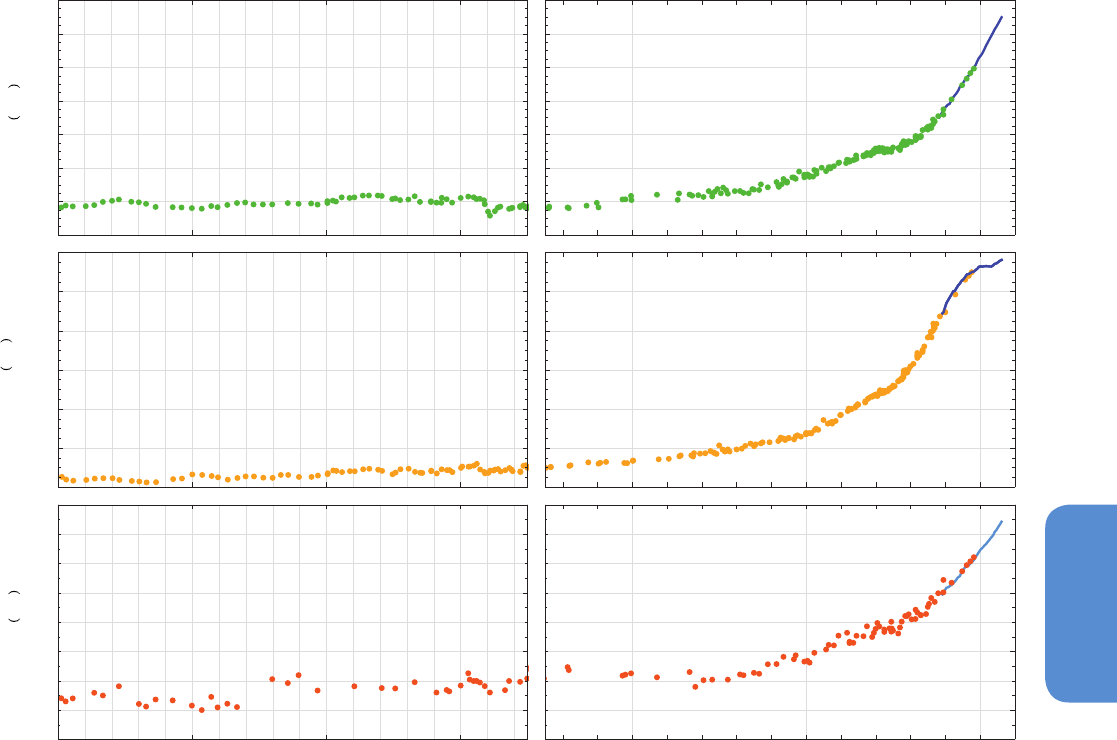
493
Carbon and Other Biogeochemical Cycles Chapter 6
6
Figure 6.11 | Atmospheric CO
2
, CH
4
, and N
2
O concentrations history over the industrial era (right) and from year 0 to the year 1750 (left), determined from air enclosed in ice cores
and firn air (colour symbols) and from direct atmospheric measurements (blue lines, measurements from the Cape Grim observatory) (MacFarling-Meure et al., 2006).
260
280
300
320
340
360
380
400
CO
2
ppm
600
800
1000
1200
1400
1600
1800
CH
4
ppb
0 1750
250
260
280
300
330
Year
1800
Year
500 1000 1500
270
290
310
320
N
2
O ppb
1900 20002020
(Trudinger et al., 2002), and the CH
4
and N
2
O growth slowed down
(MacFarling-Meure et al., 2006), possibly caused by slightly decreasing
temperatures over land in the NH (Rafelski et al., 2009).
There is substantial evidence, for example, from
13
C carbon isotopes in
atmospheric CO
2
(Keeling et al., 2005) that source/sink processes on
land generate most of the interannual variability in the atmospheric
CO
2
growth rate (Figure 6.12). The strong positive anomalies of the CO
2
growth rate in El Niño years (e.g., 1986–1987 and 1997–1998) orig-
inated in tropical latitudes (see Sections 6.3.6.3 and 6.3.2.5.4), while
the anomalies in 2003 and 2005 originated in northern mid-latitudes,
perhaps reflecting the European heat wave in 2003 (Ciais et al., 2005).
Volcanic forcing also contributes to multi-annual variability in carbon
storage on land and in the ocean (Jones and Cox, 2001; Gerber et al.,
2003; Brovkin et al., 2010; Frölicher et al., 2011).
With a very high confidence, the increase in CO
2
emissions from fossil
fuel burning and those arising from land use change are the dominant
cause of the observed increase in atmospheric CO
2
concentration. Sev-
eral lines of evidence support this conclusion:
• The observed decrease in atmospheric O
2
content over past two
decades and the lower O
2
content in the northern compared to
the SH are consistent with the burning of fossil fuels (see Figure
6.3 and Section 6.1.3.2; Keeling et al., 1996; Manning and Keeling,
2006).
• CO
2
from fossil fuels and from the land biosphere has a lower
13
C/
12
C stable isotope ratio than the CO
2
in the atmosphere. This
induces a decreasing temporal trend in the atmospheric
13
C/
12
C
ratio of atmospheric CO
2
concentration as well as, on annual aver-
age, slightly lower
13
C/
12
C values in the NH (Figure 6.3). These sig-
nals are measured in the atmosphere.
• Because fossil fuel CO
2
is devoid of radiocarbon (
14
C), reconstruc-
tions of the
14
C/C isotopic ratio of atmospheric CO
2
from tree rings
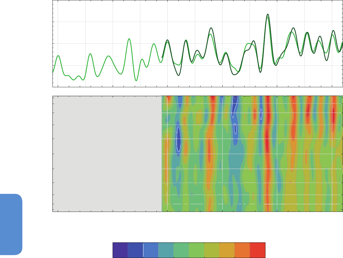
494
Chapter 6 Carbon and Other Biogeochemical Cycles
6
Figure 6.12 | (Top) Global average atmospheric CO
2
growth rate, computed from the observations of the Scripps Institution of Oceanography (SIO) network (light green line:
Keeling et al. 2005, updated)and from the marine boundary layer air reference measurements of the National Oceanic and Atmospheric Administration –Global Monitoring Division
(NOAA–GMD) network (dark green line:Conway et al., 1994; Dlugokencky and Tans, 2013b). (Bottom) Atmospheric growth rate of CO
2
as a function of latitude determined from
the National Oceanic and Atmospheric Administration–Earth System Research Laboratory (NOAA–ESRL) network, representative of stations located in the marine boundary layer
at each given latitude (Masarie and Tans, 1995; Dlugokencky and Tans, 2013b). Sufficient observations are available only since 1979.
0
1
2
3
4
1960 1970 1980 1990 2000 2010
ppm yr
-
1
(
)
ppm yr
-
1
(
)
1960 1970 1980 1990 2000 2010
90S
60S
45S
30S
15S
EQ
15N
30N
45N
60N
90N
Year
Latitude
-1 0 1 2 3 4
show a declining trend, as expected from the addition of fossil CO
2
(Stuiver and Quay, 1981; Levin et al., 2010). Yet nuclear weapon
tests in the 1950s and 1960s have been offsetting that declining
trend signal by adding
14
C to the atmosphere. Since this nuclear
weapon induced
14
C pulse in the atmosphere has been fading, the
14
C/C isotopic ratio of atmospheric CO
2
is observed to resume its
declining trend (Naegler and Levin, 2009; Graven et al., 2012).
• Most of the fossil fuel CO
2
emissions take place in the industri-
alised countries north of the equator. Consistent with this, on
annual average, atmospheric CO
2
measurement stations in the NH
record increasingly higher CO
2
concentrations than stations in the
SH, as witnessed by the observations from Mauna Loa, Hawaii, and
the South Pole (see Figure 6.3). The annually averaged concentra-
tion difference between the two stations has increased in propor-
tion of the estimated increasing difference in fossil fuel combus-
tion emissions between the hemispheres (Figure 6.13; Keeling et
al., 1989; Tans et al., 1989; Fan et al., 1999).
• The rate of CO
2
emissions from fossil fuel burning and land use
change was almost exponential, and the rate of CO
2
increase in
the atmosphere was also almost exponential and about half that
of the emissions, consistent with a large body of evidence about
changes of carbon inventory in each reservoir of the carbon cycle
presented in this chapter.
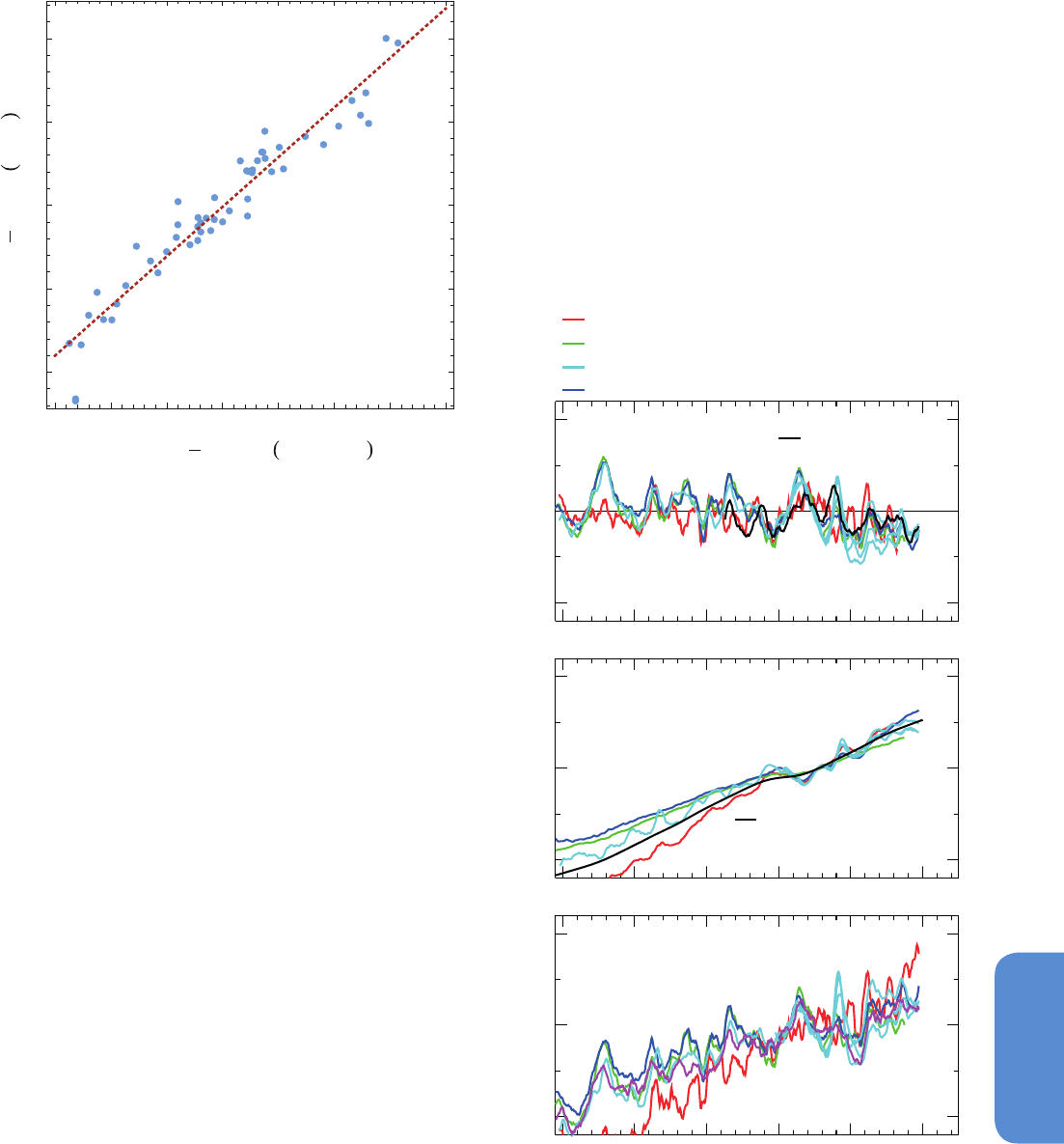
495
Carbon and Other Biogeochemical Cycles Chapter 6
6
2 3 4 5 6 7 8 9
0
1
2
3
4
Q
foss,N
Q
foss,S
PgCyr
-1
C
MLO
C
SPO
ppm
Figure 6.13 | Blue points: Annually averaged CO
2
concentration difference between
the station Mauna Loa in the Northern Hemisphere and the station South Pole in the
Southern Hemisphere (vertical axis; Keeling et al., 2005, updated) versus the difference
in fossil fuel combustion CO
2
emissions between the hemispheres (Boden et al., 2011).
Dark red dashed line: regression line fitted to the data points.
6.3.2.4 Carbon Dioxide Airborne Fraction
Until recently, the uncertainty in CO
2
emissions from land use change
emissions was large and poorly quantified which led to the use of an
airborne fraction (see Glossary) based on CO
2
emissions from fossil fuel
only (e.g., Figure 7.4 in AR4 and Figure 6.26 of this chapter). However,
reduced uncertainty of emissions from land use change and larger
agreement in its trends over time (Section 6.3.2.2) allow making use
of an airborne fraction that includes all anthropogenic emissions. The
airborne fraction will increase if emissions are too fast for the uptake
of CO
2
by the carbon sinks (Bacastow and Keeling, 1979; Gloor et al.,
2010; Raupach, 2013). It is thus controlled by changes in emissions
rates, and by changes in carbon sinks driven by rising CO
2
, changes in
climate and all other biogeochemical changes.
A positive trend in airborne fraction of ~0.3% yr
–1
relative to the mean
of 0.44 ±0.06 (or about 0.05 increase over 50 years) was found by all
recent studies (Raupach et al., 2008, and related papers; Knorr, 2009;
Gloor et al., 2010) using the airborne fraction of total anthropogenic
CO
2
emissions over the approximately 1960–2010 period (for which
the most accurate atmospheric CO
2
data are available). However, there
is no consensus on the significance of the trend because of differences
in the treatment of uncertainty and noise (Raupach et al., 2008; Knorr,
2009). There is also no consensus on the cause of the trend (Canadell
et al., 2007b; Raupach et al., 2008; Gloor et al., 2010). Land and ocean
carbon cycle model results attributing the trends of fluxes to underly-
ing processes suggest that the effect of climate change and variability
on ocean and land sinks have had a significant influence (Le Quéré et
al., 2009), including the decadal influence of volcanic eruptions (Fröli-
cher et al., 2013).
6.3.2.5 Ocean Carbon Dioxide Sink
6.3.2.5.1 Global ocean sink and decadal change
The estimated mean anthropogenic ocean CO
2
sink assessed in AR4
was 2.2 ± 0.7 PgC yr
–1
for the 1990s based on observations (McNeil et
al., 2003; Manning and Keeling, 2006; Mikaloff-Fletcher et al., 2006),
and is supported by several contemporary estimates (see Chapter 3).
Note that the uncertainty of ±0.7 PgC yr
–1
reported here (90% confi-
dence interval) is the same as the ±0.4 PgC yr
–1
uncertainty reported
in AR4 (68% confidence intervals). The uptake of anthropogenic CO
2
by the ocean is primarily a response to increasing CO
2
in the atmos-
Park et al. (2010)
b. CO effect only
2
a. Climate effect only
Assmann et al. (2010)
Graven et al. (2012)
updated from Le Quere et al. (2010)
updated from Doney et al. (2009)
updated from Khatiwala et al.
(2009)
c. CO and climate effects combined
2
Year
1960
1970
1980
1990
2000
2010
1960
1970
1980 1990
2000
2010
1960
1970 1980
1990
2000
2010
1
0
-1
1
0
-1
1
0
-1
Ocean CO sink anomalies (PgC yr )
2
-1
Figure 6.14 | Anomalies in the ocean CO
2
ocean-to-atmosphere flux in response to
(a) changes in climate, (b) increasing atmospheric CO
2
and (c) the combined effects of
increasing CO
2
and changes in climate (PgC yr
–1
). All estimates are shown as anomalies
with respect to the 1990–2000 averages. Estimates are updates from ocean models
(in colours) and from indirect methods based on observations (Khatiwala et al., 2009;
Park et al., 2010). A negative ocean-to-atmosphere flux represents a sink of CO
2
, as in
Table 6.1.

496
Chapter 6 Carbon and Other Biogeochemical Cycles
6
Method
1990s Minus 1980s
PgC yr
–1
2000s Minus 1990s
PgC yr
–1
CO
2
effects only
Khatiwala et al. (2009) Data-based
c
0.24 0.20
Mikaloff-Fletcher et al. (2006)
a
Data-based
d
0.40 0.44
Assmann et al. (2010) (to 2007 only) Model 0.28 0.35
Graven et al. (2012) Model 0.15 0.25
Doney et al. (2009) Model 0.15 0.39
Le Quéré et al. (2010) NCEP Model 0.16 0.32
Le Quéré et al. (2010) ECMWF Model — 0.39
Le Quéré et al. (2010) JPL Model — 0.32
Average
b
0.23 ± 0.15 0.33 ± 0.13
Climate effects only
Park et al. (2010) Data-based
e
— –0.15
Assmann et al. (2010) (to 2007 only) Model 0.07 0.00
Graven et al. (2012) Model 0.02 –0.27
Doney et al. (2009) Model –0.02 –0.21
Le Quéré et al. (2010) NCEP Model 0.02 –0.27
Le Quéré et al. (2010) ECMWF Model — –0.14
Le Quéré et al. (2010) JPL Model — –0.36
Average
b
0.02 ± 0.05 –0.19 ± 0.18
CO
2
and climate effects combined 0.25 ± 0.16 0.14 ± 0.22
Notes:
a
As published by Sarmiento et al. (2010).
b
Average of all estimates ±90% confidence interval. The average includes results by Le Quéré et al. (2010)–NCEP only because the other Le Quéré et al. model versions do not differ sufficiently
to be considered separately.
c
Based on observed patterns of atmospheric minus oceanic pCO
2
, assuming the difference increases with time following the increasing atmospheric CO
2
.
d
Ocean inversion, assuming constant oceanic transport through time.
e
Based on observed fit between the variability in temperature and pCO
2
, and observed variability in temperature.
ECMWF = European Centre for Medium-Range Weather Forecasts; JPL = Jet Propulsion Laboratory; NCEP = National Centers for Environmental Prediction.
Table 6.4 | Decadal changes in the ocean CO
2
sink from models and from data-based methods (a positive change between two decades means an increasing sink with time). It
is reminded that the total CO
2
sink for the 1990s is estimated at 2.2 ± 0.7 PgC yr
–1
based on observations.
phere and is limited mainly by the rate at which anthropogenic CO
2
is
transported from the surface waters into the deep ocean (Sarmiento
et al., 1992; Graven et al., 2012). This anthropogenic ocean CO
2
sink
occurs on top of a very active natural oceanic carbon cycle. Recent
climate trends, such as ocean warming, changes in ocean circulation
and changes in marine ecosystems and biogeochemical cycles, can
have affected both the anthropogenic ocean CO
2
sink as well as the
natural air–sea CO
2
fluxes. We report a decadal mean uptake of 2.0
± 0.7 PgC yr
–1
for the 1980s and of 2.3 ± 0.7 PgC yr
–1
for the 2000s
(Table 6.4). The methods used are: (1) an empirical Green’s function
approach fitted to observations of transient ocean tracers (Khatiwala
et al., 2009), (2) a model-based Green’s function approach fitted to
anthropogenic carbon reconstructions (Mikaloff-Fletcher et al., 2006),
(3) estimates based on empirical relationships between observed
ocean surface pCO
2
and temperature and salinity (Park et al., 2010)
and (4) process-based global ocean biogeochemical models forced
by observed meteorological fields (Doney et al., 2009; Assmann et al.,
2010; Le Quéré et al., 2010; Graven et al., 2012). All these different
methods suggest that in the absence of recent climate change and
climate variability, the ocean anthropogenic CO
2
sink should have
increased by 0.23 ± 0.15 PgC yr
–1
between the 1980s and the 1990s,
and by 0.33 ± 0.13 PgC yr
–1
between the 1990s and the 2000s (Figure
6.14). The decadal estimates in the ocean CO
2
sink reported in Table 6.4
as ‘CO
2
effects only’ are entirely explained by the faster rate of increase
of atmospheric CO
2
in the later decade. On the other hand, ‘climate
effects only’ in Table 6.4 are assessed to have no noticeable effect on
the sink difference between the 1980s and the 1990s (0.02 ± 0.05 PgC
yr
–1
), but are estimated to have reduced the ocean anthropogenic CO
2
sink by 0.19 ± 0.18 PgC yr
–1
between the 1990s and the 2000s (Table
6.4).
6.3.2.5.2 Regional changes in ocean dissolved inorganic carbon
Observational-based estimates for the global ocean inventory of
anthropogenic carbon are obtained from shipboard repeated hydro-
graphic cross sections (Sabine et al., 2004; Waugh et al., 2006; Khati-
wala et al., 2009). These estimates agree well among each other, with
an average value of 155 ± 30 PgC of increased dissolved inorgan-
ic carbon for the period 1750–2011 (see Chapter 3). The uptake of
anthropogenic carbon into the ocean is observed to be larger in the
high latitudes than in the tropics and subtropics over the entire Indus-
trial Era, because of the more vigorous ocean convection in the high
latitudes (Khatiwala et al., 2009). A number of ocean cross sections
have been repeated over the last decade, and the observed changes

497
Carbon and Other Biogeochemical Cycles Chapter 6
6
Table 6.5 | Regional rates of change in inorganic carbon storage from shipboard repeated hydrographic cross sections.
Section Time
Storage Rate
(mol C m
–2
yr
–1
)
Data Source
Global average (used in Table 6.1) 2007–2008 0.5 ± 0.2 Khatiwala et al. (2009)
Pacific Ocean
Section along 30°S 1992–2003 1.0 ± 0.4 Murata et al. (2007)
N of 50°S, 120°W to 180°W 1974–1996 0.9 ± 0.3 Peng et al. (2003)
154°W, 20°N to 50°S 1991–2006 0.6 ± 0.1 Sabine et al. (2008)
140°E to 170°W, 45°S to 65°S 1968–1991/1996 0.4 ± 0.2 Matear and McNeil (2003)
149° W, 4°S to 10°N 1993–2005 0.3 ± 0.1 Murata et al. (2009)
149° W, 24°N to 30°N 1993–2005 0.6 ± 0.2 Murata et al. (2009)
Northeast Pacific 1973–1991 1.3 ± 0.5 Peng et al. (2003)
~160°E, ~45°N 1997–2008 0.4 ± 0.1 Wakita et al. (2010)
North of 20°N 1994–2004/2005 0.4 ± 0.2 Sabine et al. (2008)
150°W, 20°S to 20°N 1991/1992–2006 0.3 ± 0.1 Sabine et al. (2008)
Indian Ocean
20°S to 10°S 1978–1995 0.1 Peng et al. (1998)
10°S to 5°N 1978–1995 0.7 Peng et al. (1998)
Section along 20°S 1995–2003/2004 1.0 ± 0.1 Murata et al. (2010)
Atlantic Ocean
Section along 30°S 1992/1993–2003 0.6 ± 0.1 Murata et al. (2010)
~30°W, 56°S to 15°S 1989–2005 0.8 Wanninkhof et al. (2010)
20°W, 64°N to 15°N 1993–2003 0.6 Wanninkhof et al. (2010)
~25°W, 15°N to 15°S 1993–2003 0.2 Wanninkhof et al. (2010)
40°N to 65°N 1981–1997/1999 2.2 ± 0.7 Friis et al. (2005)
20°N to 40°N 1981–2004 1.2 ± 0.3 Tanhua et al. (2007)
Nordic Seas 1981–2002/2003 0.9 ± 0.2 Olsen et al. (2006)
Sub-decadal variations
Irminger Sea 1981–1991 0.6 ± 0.4 Pérez et al. (2008)
Irminger Sea 1991–1996 2.3 ± 0.6 Pérez et al. (2008)
Irminger Sea 1997–2006 0.8 ± 0.2 Pérez et al. (2008)
in carbon storage (Table 6.5) suggest that some locations have rates
of carbon accumulation that are higher and others that are lower than
the global average estimated by Khatiwala et al. (2009). Model results
suggest that there may be an effect of climate change and variability
in the storage of total inorganic carbon in the ocean (Table 6.4), but
that this effect is small (~2 PgC over the past 50 years; Figure 6.14)
compared to the cumulative uptake of anthropogenic carbon during
the same period.
6.3.2.5.3 Interannual variability in air-sea CO
2
fluxes
The interannual variability in the global ocean CO
2
sink is estimated
to be of about ±0.2 PgC yr
–1
(Wanninkhof et al., 2013) which is small
compared to the interannual variability of the terrestrial CO
2
sink (see
Sections 6.3.2.3 and 6.3.2.6.3; Figure 6.12). In general, the ocean takes
up more CO
2
during El Niño episodes (Park et al., 2010) because of the
temporary suppression of the source of CO
2
to the atmosphere over
the eastern Pacific upwelling. Interannual variability of ~0.3 PgC yr
–1
has been reported for the North Atlantic ocean region alone (Watson
et al., 2009) but there is no agreement among estimates regarding
the exact magnitude of driving factors of air–sea CO
2
flux variability
in this region (Schuster et al., 2013). Interannual variability of 0.1 to
0.2 PgC yr
–1
was also estimated by models and one atmospheric inver-
sion in the Southern Ocean (Le Quéré et al., 2007), possibly driven by
the Southern Annular Mode of climate variability (Lenton and Matear,
2007; Lovenduski et al., 2007; Lourantou and Metzl, 2011).
6.3.2.5.4 Regional ocean carbon dioxide partial pressure trends
Observations of the partial pressure of CO
2
at the ocean surface (pCO
2
)
show that ocean pCO
2
has been increasing generally at about the same
rate as CO
2
in the atmosphere when averaged over large ocean regions
during the past two to three decades (Yoshikawa-Inoue and Ishii, 2005;
Takahashi et al., 2009; McKinley et al., 2011). However, analyses of
regional observations highlight substantial regional and temporal var-
iations around the mean trend.
In the North Atlantic, repeated observations show ocean pCO
2
increas-
ing regionally either at the same rate or faster than atmospheric CO
2
between about 1990 and 2006 (Schuster et al., 2009), thus indicating
a constant or decreasing sink for CO
2
in that region, in contrast to the
increasing sink expected from the response of the ocean to increasing

498
Chapter 6 Carbon and Other Biogeochemical Cycles
6
atmospheric CO
2
alone. The anomalous North Atlantic trends appear
to be related to sea surface warming and its effect on solubility (Cor-
bière et al., 2007) and/or changes in ocean circulation (Schuster and
Watson, 2007; Schuster et al., 2009) and deep convection (Metzl et al.,
2010). Recent changes have been associated with decadal variability
in the North Atlantic Oscillation (NAO) and the Atlantic Multidecadal
Variability (AMV) (Thomas et al., 2007; Ullman et al., 2009; McKinley et
al., 2011; Tjiputra et al., 2012). A systematic analysis of trends estimat-
ed in this region show no agreement regarding the drivers of change
(Schuster et al., 2013).
In the Southern Ocean, an approximately constant sink was inferred
from atmospheric (Le Quéré et al., 2007) and oceanic (Metzl, 2009;
Takahashi et al., 2009) CO
2
observations but the uncertainties are large
(Law et al., 2008). Most ocean biogeochemistry models reproduce the
constant sink and attribute it as a response to an increase in Southern
Ocean winds driving increased upwards transport of carbon-rich deep
waters (Lenton and Matear, 2007; Verdy et al., 2007; Lovenduski et al.,
2008; Le Quéré et al., 2010). The increase in winds has been attribut-
ed to the depletion of stratospheric ozone (Thompson and Solomon,
2002) with a contribution from GHGs (Fyfe and Saenko, 2006).
Large decadal variability has been observed in the Equatorial Pacific
(Ishii et al., 2009) associated with changes in the phasing of the Pacif-
ic Decadal Oscillation (see Glossary) and its impact on gas transfer
velocity (Feely et al., 2006; Valsala et al., 2012). By contrast, ocean
pCO
2
appears to have increased at a slower rate than atmospheric CO
2
(thus a growing ocean CO
2
sink in that region) in the northern North
Pacific Ocean (Takahashi et al., 2006). There is less evidence available
to attribute the observed changes in other regions to changes in under-
lying processes or climate change and variability.
6.3.2.5.5 Processes driving variability and trends in air–sea
carbon dioxide fluxes
Three type of processes are estimated to have an important effect on
the air–sea CO
2
fluxes on century time scales: (1) the dissolution of
CO
2
at the ocean surface and its chemical equilibrium with other forms
of carbon in the ocean (mainly carbonate and bicarbonate), (2) the
transport of carbon between the surface and the intermediate and
deep ocean and (3) changes in the cycling of carbon through marine
ecosystem processes (the ocean biological pump; see Section 6.1.1.1).
The surface dissolution and equilibration of CO
2
with the atmosphere
is well understood and quantified. It varies with the surface ocean con-
ditions, in particular with temperature (solubility effect) and alkalinity.
The capacity of the ocean to take up additional CO
2
for a given alka-
linity decreases at higher temperature (4.23% per degree warming;
Takahashi et al., 1993) and at elevated CO
2
concentrations (about 15%
per 100 ppm, computed from the so called Revelle factor; Revelle and
Suess, 1957).
Recent changes in nutrient supply in the ocean are also thought to
have changed the export of organic carbon from biological process-
es below the surface layer, and thus the ocean CO
2
sink (Duce et al.,
2008). Anthropogenic reactive nitrogen Nr (see Box 6.2) entering the
ocean via atmospheric deposition or rivers acts as a fertiliser and
may enhance carbon export to depth and hence the CO
2
sink. This Nr
contribution has been estimated to be between 0.1 and 0.4 PgC yr
–1
around the year 2000 using models (Duce et al., 2008; Reay et al.,
2008; Krishnamurthy et al., 2009; Suntharalingam et al., 2012). Simi-
larly, increases in iron deposition over the ocean from dust generated
by human activity is estimated to have enhanced the ocean cumulative
CO
2
uptake by 8 PgC during the 20th century (or about 0.05 PgC yr
–1
in
the past decades) (Mahowald et al., 2010). Although changes in ocean
circulation and in global biogeochemical drivers have the potential to
alter the ocean carbon fluxes through changes in marine ecosystems,
modelling studies show only small variability in ocean biological pump,
which has not significantly impacted the response of the ocean carbon
cycle over the recent period (Bennington et al., 2009).
Model studies suggest that the response of the air–sea CO
2
fluxes to
climate change and variability in recent decades has decreased the
rate at which anthropogenic CO
2
is absorbed by the ocean (Sarmiento
et al. (2010); Figure 6.14 and Table 6.4). This result is robust to the
model or climate forcing used (Figure 6.13), but no formal attribution
to anthropogenic climate change has been made. There is insuffi-
cient data coverage to separate the impact of climate change on the
global ocean CO
2
sink directly from observations, though the regional
trends described in Section 6.3.2.5.4 suggest that surface ocean pCO
2
responds to changes in ocean properties in a significant and measur-
able way.
6.3.2.5.6 Model evaluation of global and regional ocean
carbon balance
Ocean process-based carbon cycle models are capable of reproduc-
ing the mean air–sea fluxes of CO
2
derived from pCO
2
observations
(Takahashi et al., 2009), including their general patterns and amplitude
(Sarmiento et al., 2000), the anthropogenic uptake of CO
2
(Orr et al.,
2001; Wanninkhof et al., 2013) and the regional distribution of air–sea
fluxes (Gruber et al., 2009). The spread between different model results
for air–sea CO
2
fluxes is the largest in the Southern Ocean (Matsu-
moto et al., 2004), where intense convection occurs. Tracer observa-
tions (Schmittner et al., 2009) and water mass analysis (Iudicone et al.,
2011) have been used to reduce the model uncertainty associated with
this process and improve the simulation of carbon fluxes. The models
reproduce the observed seasonal cycle of pCO
2
in the sub-tropics but
generally do poorly in sub-polar regions where the balance of process-
es is more difficult to simulate well (McKinley et al., 2006; Schuster
et al., 2013). Less information is available to evaluate specifically the
representation of biological fluxes in the models, outside of their real-
istic representation of surface ocean chlorophyll distributions. Ocean
process-based carbon cycle models used in AR5 reproduce the relative-
ly small interannual variability inferred from observations (Figure 6.12;
Wanninkhof et al., 2013). See also Section 9.4.5.
Sensitivity of modelled air–sea fluxes to CO
2
. Data-based studies esti-
mated a cumulative carbon uptake of ~155 ± 30 PgC across stud-
ies for the 1750–2011 time period (Sabine et al., 2004; Waugh et al.,
2006; Khatiwala et al., 2009), a mean anthropogenic CO
2
sink of 2.2
± 0.7 PgC yr
–1
for the 1990s, and decadal trends of 0.13 PgC yr
–1
per
decade during the two decades 1990–2009 (Wanninkhof et al., 2013;
from atmospheric inversions), respectively. Models that have estimat-
ed these quantities give a total ocean uptake of 170 ± 25 PgC for

499
Carbon and Other Biogeochemical Cycles Chapter 6
6
1750–2011 (from the model ensemble of Orr et al., (2005) until 1994,
plus an additional 40 PgC from estimates in Table 6.4 for 1995–2011),
a mean anthropogenic CO
2
sink of 2.1 ± 0.6 PgC yr
–1
for 1990–1999 (Le
Quéré et al., 2013) and a decadal trend of 0.14 PgC yr
–1
per decade for
1990–2009 (Wanninkhof et al., 2013). Therefore, although the ocean
models do not reproduce all the details of the regional structure and
changes in air–sea CO
2
fluxes, their globally integrated ocean CO
2
sink
and decadal rate of change of this sink is in good agreement with the
available observations.
Sensitivity of modelled air–sea fluxes to climate. The relationship
between air–sea CO
2
flux and climate is strongly dependent on the
oceanic region and on the time scale. Ocean carbon cycle models of
the type used in AR5 estimate a reduction in cumulative ocean CO
2
uptake of 1.6 to 5.4 PgC over the period 1959–2008 (1.5 to 5.4%) in
response to climate change and variability compared to simulations
with no changes in climate (Figure 6.14), partly due to changes in
the equatorial Pacific and to changes in the Southern Ocean. The only
observation-based estimate available to evaluate the climate response
of the global air–sea CO
2
flux is from Park et al. (2010), which is at
the low end of the model estimate for the past two decades (Table
6.4). However, this estimate does not include the nonlinear effects of
changes in ocean circulation and warming on the global air–sea CO
2
flux, which could amplify the response of the ocean CO
2
sink to climate
by 20 to 30% (Le Quéré et al., 2010; Zickfeld et al., 2011).
Processes missing in ocean models. The most important processes
missing in ocean carbon cycle models used in the AR5 are those rep-
resenting explicitly small-scale physical circulation (e.g., eddies, brine
formation), which are parameterised in models. These processes have
an important influence on the vertical transport of water, heat, salt
and carbon (Loose and Schlosser, 2011; Sallée et al., 2012). In particu-
lar, changes in vertical transport in the Southern Ocean are thought
to explain part of the changes in atmospheric CO
2
between glacial
and interglacial conditions, a signal that is not entirely reproduced by
models (Section 6.2) suggesting that the sensitivity of ocean models
could be underestimated.
Processes related to marine ecosystems in global ocean models are
also limited to the simulation of lower trophic levels, with crude
parameterizations for sinking processes, bacterial and other loss pro-
cesses at the surface and in the ocean interior and their temperature
dependence (Kwon et al., 2009). Projected changes in carbon fluxes
from the response of marine ecosystems to changes in temperature
(Beaugrand et al., 2010), ocean acidification (Riebesell et al., 2009)
(see Glossary) and pressure from fisheries (Pershing et al., 2010) are
all considered potentially important, though not yet quantified. Several
processes have been specifically identified that could lead to changes
in the ocean CO
2
sink, in particular the temperature effects on marine
ecosystem processes (Riebesell et al., 2009; Taucher and Oschlies,
2011) and the variable nutrient ratios induced by ocean acidification
or ecosystem changes (Tagliabue et al., 2011). Coastal ocean process-
es are also poorly represented in global and may influence the ocean
CO
2
sink. Nevertheless, the fit of ocean model results to the integrated
CO
2
sink and decadal trends discussed above suggestthat, up to now,
the missing processes have not had a dominant effect on ocean CO
2
beyond the limits of the uncertainty of the data.
6.3.2.6 Land Carbon Dioxide Sink
6.3.2.6.1 Global residual land sink and atmosphere-to-land
carbon dioxide flux
The residual land CO
2
sink, that is, the uptake of CO
2
in ecosystems
excluding the effects of land use change, is 1.5 ± 1.1, 2.6 ± 1.2 and 2.6
± 1.2 PgC yr
–1
for the 1980s, 1990s and 2000s, respectively (Table 6.1).
After including the net land use change emissions, the atmosphere-
to-land flux of CO
2
(Table 6.1) corresponds to a net sink of CO
2
by all
terrestrial ecosystems. This sink has intensified globally from a neutral
CO
2
flux of 0.1 ± 0.8 PgC yr
–1
in the 1980s to a net CO
2
sink of 1.1 ±
0.9 PgC yr
–1
and 1.5 ± 0.9 PgC yr
–1
during the 1990s and 2000s, respec-
tively (Table 6.1; Sarmiento et al., 2010). This growing land sink is also
supported by an atmospheric inversion (Gurney and Eckels, 2011) and
by process-based models (Le Quéré et al., 2009).
6.3.2.6.2 Regional atmosphere-to-land carbon dioxide fluxes
The results from atmospheric CO
2
inversions, terrestrial ecosystem
models and forest inventories consistently show that there is a large
net CO
2
sink in the northern extratropics, albeit the very limited availa-
bility of observations in the tropics (Jacobson et al., 2007; Gurney and
Eckels, 2011; Pan et al., 2011). Inversion estimates of atmosphere–land
CO
2
fluxes show net atmosphere-to-land CO
2
flux estimates ranging
from neutral to a net source of 0.5 to 1.0 PgC yr
–1
(Jacobson et al.,
2007; Gurney and Eckels, 2011) (Figure 6.15). However, Stephens et al.
(2007) selected from an ensemble of inversion models those that were
consistent with independent aircraft cross-validation data, and con-
strained an atmosphere-to-land CO
2
flux of 0.1 ± 0.8 PgC yr
–1
during
the period 1992–1996, and a NH net CO
2
sink of 1.5 ± 0.6 PgC yr
–1
.
These results shows that after subtracting emissions from land use
change, tropical land ecosystems might also be large CO
2
sinks.
Based on repeated forest biomass inventory data, estimated soil
carbon changes, and CO
2
emissions from land use change from the
bookkeeping method of Houghton et al. (2012), Pan et al. (2011) esti-
mated a global forest carbon accumulation of 0.5 ± 0.1 PgCyr
–1
in
boreal forests, and of 0.8 ± 0.1 PgC yr
–1
in temperate forests for the
period 2000–2007. Tropical forests were found to be near neutral with
net emissions from land use change being compensated by sinks in
established tropical forests (forests not affected by land use change),
therefore consistent with the Stephens et al. (2007) inversion estimate
of tropical atmosphere–land CO
2
fluxes.
Since AR4, a number of studies have compared and attempted to rec-
oncile regional atmosphere-to-land CO
2
flux estimates from multiple
approaches and so providing further spatial resolution of the regional
contributions of carbon sources and sinks (Table 6.6). A synthesis of
regional contributions estimated a 1.7 PgC yr
–1
sink in the NH regions
above 20°N with consistent estimates from terrestrial models and
inventories (uncertainty: ±0.3 PgC yr
–1
) and atmospheric CO
2
inver-
sions (uncertainty: ±0.7 PgC yr
–1
) (Ciais et al., 2010).
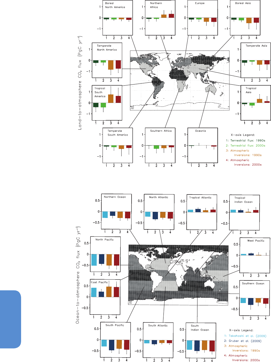
500
Chapter 6 Carbon and Other Biogeochemical Cycles
6
Figure 6.15 | (Top) Bar plots showing decadal average CO
2
fluxes for 11 land regions (1) as estimated by 10 different atmospheric CO
2
inversions for the 1990s (yellow) and
2000s (red) (Peylin et al., 2013; data source: http://transcom.lsce.ipsl.fr/), and (2) as simulated by 10 dynamic vegetation models (DGVMs) for the 1990s (green) and 2000s (light
green) (Piao et al., 2013; data source: http://www-lscedods.cea.fr/invsat/RECCAP/). The divisions of land regions are shown in the map. (Bottom) Bar plots showing decadal average
CO
2
fluxes for 11 ocean regions (1) as estimated by 10 different atmospheric CO
2
inversions for the 1990s (yellow) and 2000s (red) (data source: http://transcom.lsce.ipsl.fr/), (2)
inversion of contemporary interior ocean carbon measurements using 10 ocean transport models (dark blue) (Gruber et al., 2009) and (3) surface ocean pCO
2
measurements based
air-sea exchange climatology (Takahashi et al., 2009). The divisions of 11 ocean regions are shown in the map.

501
Carbon and Other Biogeochemical Cycles Chapter 6
6
Table 6.6 | Regional CO
2
budgets using top-down estimates (atmospheric inversions) and bottom-up estimates (inventory data, biogeochemical modelling, eddy-covariance),
excluding fossil fuel emissions. A positive sign indicates a flux from the atmosphere to the land (i.e., a land sink).
Region CO
2
Sink (PgC yr
–1
) Uncertainty
a
Period Reference
Artic Tundra 0.1 ±0.3
b
2000–2006 McGuire et al. (2012)
Australia 0.04 ±0.03 1990–2009 Haverd et al. (2013)
East Asia 0.25 ±0.1 1990–2009 Piao et al. (2012)
Europe 0.9 ±0.2 2001–2005 Luyssaert et al. (2012)
North America 0.6 ±0.02 2000–2005 King et al. (2012)
Russian Federation 0.6 –0.3 to –1.3 1990–2007 Dolman et al. (2012)
South Asia 0.15 ±0.24 2000–2009 Patra et al. (2013)
South America –0.3 ±0.3 2000–2005 Gloor et al. (2012)
Notes:
a
One standard deviation from mean unless indicated otherwise.
b
Based on range provided.
6.3.2.6.3 Interannual variability in atmosphere-to-land carbon
dioxide fluxes
The interannual variability of the residual land sink shown in Figures
6.12 and 6.16 accounts for most of the interannual variability of the
atmospheric CO
2
growth rate (see Section 6.3.2.3). Atmospheric CO
2
inversion results suggest that tropical land ecosystems dominate the
global CO
2
variability, with positive anomalies during El Niño episodes
(Bousquet et al., 2000; Rödenbeck et al., 2003; Baker et al., 2006),
which is consistent with the results of one inversion of atmospher-
ic
13
C and CO
2
measurements (Rayner et al., 2008). A combined El
Niño-Southern Oscillation (ENSO)–Volcanic index time series explains
75% of the observed variability (Raupach et al., 2008). A positive phase
of ENSO (El Niño, see Glossary) is generally associated with enhanced
land CO
2
source, and a negative phase (La Niña) with enhanced land
CO
2
sink (Jones and Cox, 2001; Peylin et al., 2005). Observations from
eddy covariance networks suggest that interannual carbon flux varia-
bility in the tropics and temperate regions is dominated by precipita-
tion, while boreal ecosystem fluxes are more sensitive to temperature
and shortwave radiation variation (Jung et al., 2011), in agreement
with the results from process-based terrestrial ecosystem models (Piao
et al., 2009a). Terrestrial biogeochemical models suggest that inter-
annual net biome productivity (NBP) variability is dominated by GPP
(see Glossary) rather than terrestrial ecosystem respiration (Piao et al.,
2009b; Jung et al., 2011).
6.3.2.6.4 Carbon fluxes from inland water
Global analyses estimate that inland waters receive about 1.7 to 2.7
PgC yr
–1
emitted by soils to rivers headstreams, of which, 0.2 to 0.6
PgC yr
–1
is buried in aquatic sediments, 0.8 to 1.2 PgC yr
–1
returns to
the atmosphere as CO
2
, and 0.9 PgC yr
–1
is delivered to the ocean (Cole
et al., 2007; Battin et al., 2009; Aufdenkampe et al., 2011). Estimates
of the transport of carbon from land ecosystems to the coastal ocean
by rivers are ~0.2 PgC yr
–1
for Dissolved Organic Carbon (DOC), 0.3
PgC yr
–1
for Dissolved Inorganic Carbon (DIC), and 0.1 to 0.4 PgC yr
–1
for Particulate Organic Carbon (POC) (Seitzinger et al., 2005; Syvitski
et al., 2005; Mayorga et al., 2010). For the DIC fluxes, only about two-
thirds of it originates from atmospheric CO
2
and the rest of the carbon
is supplied by weathered carbonate rocks (Suchet and Probst, 1995;
Gaillardet et al., 1999; Oh and Raymond, 2006; Hartmann et al., 2009).
Regional DIC concentrations in rivers has increased during the Indus-
trial Era (Oh and Raymond, 2006; Hamilton et al., 2007; Perrin et al.,
2008). Agricultural practices coupled with climate change can lead to
large increases in regional scale DIC export in watersheds with a large
agricultural footprint (Raymond et al., 2008). Furthermore, region-
al urbanization also elevates DIC fluxes in rivers (Baker et al., 2008;
Barnes and Raymond, 2009), which suggests that anthropogenic activ-
ities have contributed a significant portion of the annual global river
DIC flux to the ocean.
Land clearing and management are thought to produce an acceleration
of POC transport, much of which is trapped in alluvial and colluvial dep-
osition zones, lakes, reservoirs and wetlands (Stallard, 1998; Smith et
al., 2001b; Syvitski et al., 2005). Numerous studies have demonstrated
an increase in the concentration of DOC in rivers in the northeastern
United States and northern/central Europe over the past two to four
decades (Worrall et al., 2003; Evans et al., 2005; Findlay, 2005; Mon-
teith et al., 2007; Lepistö et al., 2008). Owing to the important role of
wetlands in DOC production, the mobilization of DOC due to human-in-
duced changes in wetlands probably represents an important cause
of changes in global river DOC fluxes to date (Seitzinger et al., 2005),
although a global estimate of this alteration is not available. A robust
partitioning between natural and anthropogenic carbon fluxes in fresh-
water systems is not yet possible, nor a quantification of the ultimate
fate of carbon delivered by rivers to the coastal and open oceans.
6.3.2.6.5 Processes driving terrestrial atmosphere-to-land
carbon dioxide fluxes
Assessment of experimental data, observations and model results sug-
gests that the main processes responsible for the residual land sink
include the CO
2
fertilisation effect on photosynthesis (see Box 6.3),
nitrogen fertilisation by increased deposition (Norby, 1998; Thornton
et al., 2007; Bonan and Levis, 2010; Zaehle and Dalmonech, 2011)
and climate effects (Nemani et al., 2003; Gloor et al., 2009). It is likely
that reactive nitrogen deposition over land currently increases natu-
ral CO
2
in particular in forests, but the magnitude of this effect varies
between regions (Norby, 1998; Thornton et al., 2007; Bonan and Levis,
2010; Zaehle and Dalmonech, 2011). Processes responsible for the
net atmosphere-to-land CO
2
sink on terrestrial ecosystems include,
in addition, forest regrowth and afforestation (Myneni et al., 2001;

502
Chapter 6 Carbon and Other Biogeochemical Cycles
6
Pacala et al., 2001; Houghton, 2010; Bellassen et al., 2011; Williams et
al., 2012a), changes in forest management and reduced harvest rates
(Nabuurs et al., 2008).
Process attribution of the global land CO
2
sink is difficult due to lim-
ited availability of global data sets and biogeochemical models that
include all major processes. However, regional studies shed light on
key drivers and their interactions. The European and North American
carbon sinks are explained by the combination of forest regrowth in
abandoned lands and decreased forest harvest along with the fertilis-
ation effects of rising CO
2
and nitrogen deposition (Pacala et al., 2001;
Ciais et al., 2008; Sutton et al., 2008; Schulze et al., 2010; Bellassen et
al., 2011; Williams et al., 2012a). In the tropics, there is evidence from
forest inventories that increasing forest growth rates are not explained
by the natural recovery from disturbances, suggesting that increasing
atmospheric CO
2
and climate change play a role in the observed sink
in established forests (Lewis et al., 2009; Pan et al., 2011). There is also
recent evidence of tropical nitrogen deposition becoming more notable
although its effects on the net carbon balance have not been assessed
(Hietz et al., 2011).
The land carbon cycle is very sensitive to climate changes (e.g., precip-
itation, temperature, diffuse vs. direct radiation), and thus the changes
in the physical climate from increasing GHGs as well as in the diffuse
fraction of sunlight are likely to be causing significant changes in the
carbon cycle (Jones et al., 2001; Friedlingstein et al., 2006; Mercado et
Box 6.3 | The Carbon Dioxide Fertilisation Effect
Elevated atmospheric CO
2
concentrations lead to higher leaf photosynthesis and reduced canopy transpiration, which in turn lead to
increased plant water use efficiency and reduced fluxes of surface latent heat. The increase in leaf photosynthesis with rising CO
2
, the
so-called CO
2
fertilisation effect, plays a dominant role in terrestrial biogeochemical models to explain the global land carbon sink
(Sitch et al., 2008), yet it is one of most unconstrained process in those models.
Field experiments provide a direct evidence of increased photosynthesis rates and water use efficiency (plant carbon gains per unit of
water loss from transpiration) in plants growing under elevated CO
2
. These physiological changes translate into a broad range of higher
plant carbon accumulation in more than two-thirds of the experiments and with increased net primary productivity (NPP) of about 20
to 25% at double CO
2
from pre-industrial concentrations (Ainsworth and Long, 2004; Luo et al., 2004, 2006; Nowak et al., 2004; Norby
et al., 2005;Canadell et al., 2007a; Denman et al., 2007; Ainsworth et al., 2012; Wang et al., 2012a). Since the AR4, new evidence is
available from long-term Free-air CO
2
Enrichment (FACE) experiments in temperate ecosystems showing the capacity of ecosystems
exposed to elevated CO
2
to sustain higher rates of carbon accumulation over multiple years (Liberloo et al., 2009; McCarthy et al., 2010;
Aranjuelo et al., 2011; Dawes et al., 2011; Lee et al., 2011; Zak et al., 2011). However, FACE experiments also show the diminishing or
lack of CO
2
fertilisation effect in some ecosystems and for some plant species (Dukes et al., 2005; Adair et al., 2009; Bader et al., 2009;
Norby et al., 2010; Newingham et al., 2013). This lack of response occurs despite increased water use efficiency, also confirmed with
tree ring evidence (Gedalof and Berg, 2010; Peñuelas et al., 2011).
Nutrient limitation is hypothesized as primary cause for reduced or lack of CO
2
fertilisation effect observed on NPP in some experi-
ments (Luo et al., 2004; Dukes et al., 2005; Finzi et al., 2007; Norby et al., 2010). Nitrogen and phosphorus are very likely to play the
most important role in this limitation of the CO
2
fertilisation effect on NPP, with nitrogen limitation prevalent in temperate and boreal
ecosystems, and phosphorus limitation in the tropics (Luo et al., 2004; Vitousek et al., 2010; Wang et al., 2010a; Goll et al., 2012).
Micronutrients interact in diverse ways with other nutrients in constraining NPP such as molybdenum and phosphorus in the tropics
(Wurzburger et al., 2012). Thus, with high confidence, the CO
2
fertilisation effect will lead to enhanced NPP, but significant uncertainties
remain on the magnitude of this effect, given the lack of experiments outside of temperate climates.
al., 2009). Changes in the climate are also associated with disturbanc-
es such as fires, insect damage, storms, droughts and heat waves which
are already significant processes of interannual variability and possibly
trends of regional land carbon fluxes (Page et al., 2002; Ciais et al.,
2005; Chambers et al., 2007; Kurz et al., 2008b; Clark et al., 2010; van
der Werf et al., 2010; Lewis et al., 2011) (see Section 6.3.2.2).
Warming (and possibly the CO
2
fertilisation effect) has also been cor-
related with global trends in satellite greenness observations, which
resulted in an estimated 6% increase of global NPP, or the accumu-
lation of 3.4 PgC on land over the period 1982–1999 (Nemani et al.,
2003). This enhanced NPP was attributed to the relaxation of climatic
constraints to plant growth, particularly in high latitudes. Concomi-
tant to the increased of NPP with warming, global soil respiration also
increased between 1989 and 2008 (Bond-Lamberty and Thomson,
2010), reducing the magnitude of the net land sink. A recent study
suggests a declining NPP trend over 2000–2009 (Zhao and Running,
2010) although the model used to reconstruct NPP trends from satel-
lite observation has not been widely accepted (Medlyn, 2011; Samanta
et al., 2011).
6.3.2.6.6 Model evaluation of global and regional terrestrial
carbon balance
Evaluation of global process-based land carbon models was performed
against ground and satellite observations including (1) measured CO
2

503
Carbon and Other Biogeochemical Cycles Chapter 6
6
fluxes and carbon storage change at particular sites around the world,
in particular sites from the Fluxnet global network (Baldocchi et al.,
2001; Jung et al., 2007; Stöckli et al., 2008; Schwalm et al., 2010; Tan
et al., 2010), (2) observed spatio-temporal change in leaf area index
(LAI) (Lucht et al., 2002; Piao et al., 2006) and (3) interannual and
seasonal change in atmospheric CO
2
(Randerson et al., 2009; Cadule
et al., 2010).
Figure 6.16 compares the global land CO
2
sink driven by climate
change and rising CO
2
as simulated by different process based carbon
cycle models (without land use change), with the residual land sink
computed as the sum of fossil fuel and cement emissions and land use
change emissions minus the sum of CO
2
growth rate and ocean sink
(Le Quéré et al., 2009; Friedlingstein et al., 2010). Although these two
quantities are not the same, the multi-model mean reproduces well
the trend and interannual variability of the residual land sink which is
dominated by climate variability and climate trends and CO
2
, respec-
tively, both represented in models (Table 6.7). Limited availability of
in situ measurements, particularly in the tropics, limits the progress
towards reducing uncertainty on model parameterizations.
Regional and local measurements can be used to evaluate and improve
global models. Regionally, forest inventory data show that the forest
carbon sink density over Europe is of –89 ± 19 gC m
–2
yr
–1
, which
Table 6.7 | Estimates of the land CO
2
sink from process-based terrestrial ecosystem models driven by rising CO
2
and by changes in climate. The land sink simulated by these models
is close to but not identical to the terrestrial CO
2
sink from Table 6.1 because the models calculate the effect of CO
2
and climate over managed land, and many do not include
nitrogen limitation and disturbances.
Model Name Nitrogen Limitation
Natural Fire CO
2
Emissions
1980–1989 1990–1999 2000–2009
(Yes/No) (Yes/No) PgC yr
–1
PgC yr
–1
PgC yr
–1
CLM4C
b,c
No Yes 1.98 2.11 2.64
CLM4CN
b,c
Yes Yes 1.27 1.25 1.67
Hyland
d
No No 2.21 2.92 3.99
LPJ
e
No Yes 1.14 1.90 2.60
LPJ_GUESS
f
No Yes 1.15 1.54 2.07
OCN
g
Yes No 1.75 2.18 2.36
ORC
h
No No 2.08 3.05 3.74
SDGVM
i
Yes Yes 1.25 1.95 2.30
TRIFFID
j
No No 1.85 2.52 3.00
VEGAS
k
No No 1.40 1.68 1.89
Average
a
1.61 ± 0.65 2.11 ± 0.93 2.63 ± 1.22
Notes:
a
Average of all models ±90% confidence interval.
b
Oleson et al. (2010).
c
Lawrence et al. (2011).
d
Levy et al. (2004).
e
Sitch et al. (2003).
f
Smith et al. (2001a).
g
Zaehle and Friend (2010).
h
Krinner et al. (2005).
is compatible with model estimates with afforestation (–63 gC m
–2
yr
–1
; Luyssaert et al., 2010), while modelled NPP was 43% larger than
the inventory estimate. In North America, the ability of 22 terrestrial
carbon cycle models to simulate the seasonal cycle of land–atmos-
phere CO
2
exchange from 44 eddy covariance flux towers was poor
with a difference between observations and simulations of 10 times
the observational uncertainty (Schwalm et al., 2010). Model short-
comings included spring phenology, soil thaw, snow pack melting
and lag responses to extreme climate events (Keenan et al., 2012). In
China, the magnitude of the carbon sink estimated by five terrestrial
ecosystem models (–0.22 to –0.13 PgC yr
–1
) was comparable to the
observation-based estimate (–0.18 ± 0.73 PgC yr
–1
; Piao et al., 2009a),
but modelled interannual variation was weakly correlated to observed
regional land–atmosphere CO
2
fluxes (Piao et al., 2011).
Sensitivity of the terrestrial carbon cycle to rising atmospheric carbon
dioxide. An inter-comparison of 10 process-based models showed
increased NPP by 3% to 10% over the last three decades, during which
CO
2
increased by ~50 ppm (Piao et al., 2013). These results are con-
sistent within the broad range of responses from experimental studies
(see Box 6.3). However, Hickler et al. (2008) suggested that currently
available FACE results (largely from temperate regions) are not appli-
cable to vegetation globally because there may be large spatial heter-
ogeneity in vegetation responses to CO
2
fertilisation.
All of these models run are forced by rising CO
2
concentration and time-varying historical reconstructed weather and climate fields using the same protocol from the TRENDY project (Piao et al.,
2013). (http://www.globalcarbonproject.org/global/pdf/DynamicVegetationModels.pdf).
CLM4C = Community Land Model for Carbon; CLM4CN = Community Land Model for Carbon–Nitrogen; GUESS = General Ecosystem Simulator; LPJ = Lund-Potsdam-Jena Dynamic Global Vegeta-
tion Model; OCN = Cycling of Carbon and Nitrogen on land, derived from ORCHIDEE model; ORC = ORCHIDEE, ORganizing Carbon and Hydrology in Dynamic EcosystEms model; SDGVM = Sheffield
Dynamic Global Vegetation Model; TRIFFID = Top-down Representation of Interactive Foliage and Flora Including Dynamics; VEGAS = VEgetation-Global-Atmosphere-Soil terrestrial carbon cycle
model.
i
Woodward and Lomas (2004).
j
Cox (2001).
k
Zeng (2003).
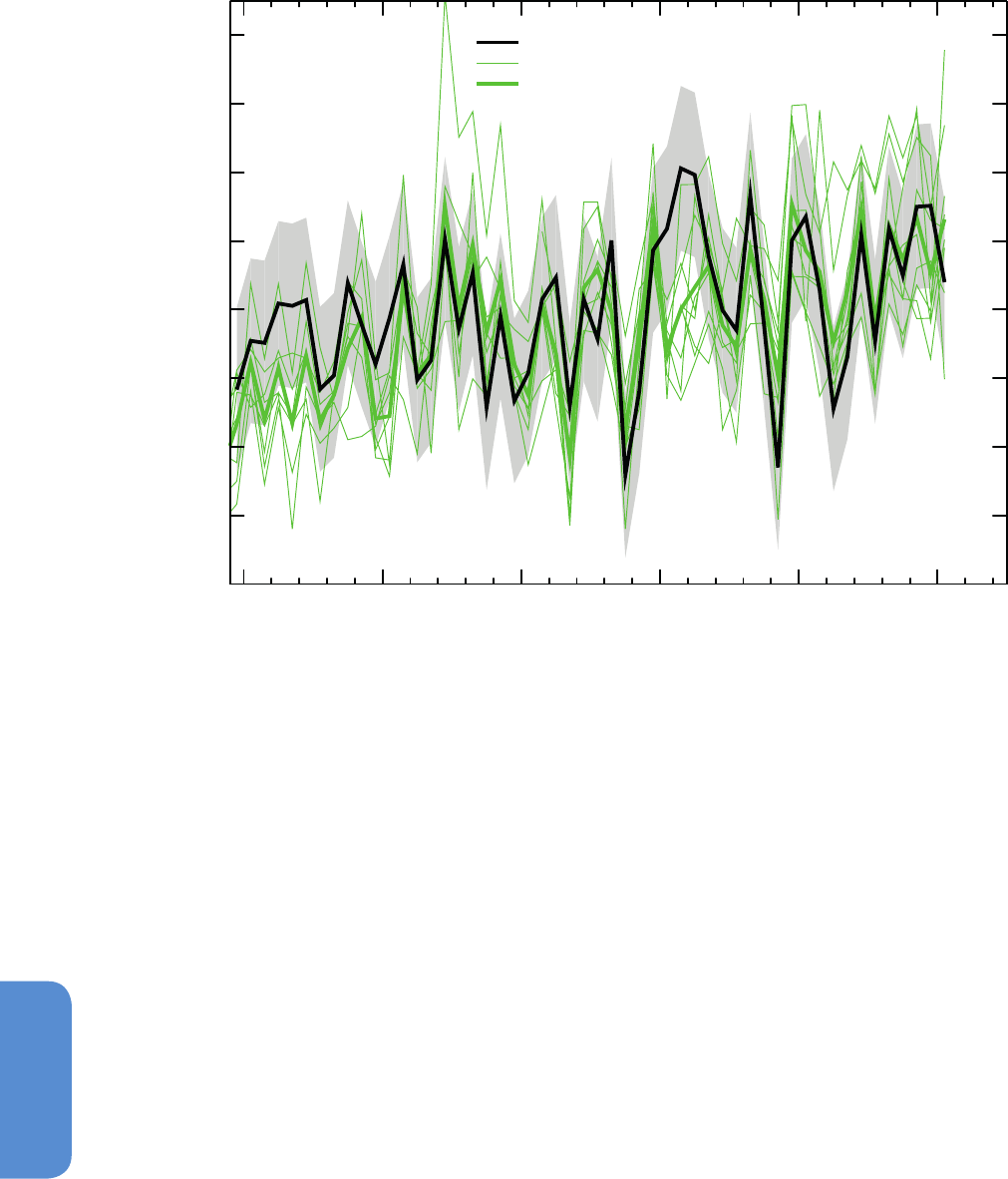
504
Chapter 6 Carbon and Other Biogeochemical Cycles
6
Year
Terrestrial CO sink (PgC yr
)
2
-1
6
5
4
3
2
1
0
-1
-2
1960 1970 1980 1990 2000 2010
Residual terrestrial sink (Table 6.1)
Process models (Table 6.6)
Process model average
Figure 6.16 | The black line and gray shading represent the estimated value of the residual land sink (PgC yr
–1
) and its uncertainty from Table 6.1, which is calculated from the dif-
ference between emissions from fossil fuel and land use change plus emissions from net land use change, minus the atmospheric growth rate and the ocean sink. The atmosphere-
to-land flux simulated by process land ecosystem models from Table 6.7 are shown in thin green, and their average in thick green. A positive atmosphere-to-land flux represents a
sink of CO
2
. The definition of the atmosphere-to-land flux simulated by these models is close to but not identical to the residual land sink from Table 6.1 (see Table 6.7).
Sensitivity of terrestrial carbon cycle to climate trends and variability.
Warming exerts a direct control on the net land–atmosphere CO
2
exchange because both photosynthesis and respiration are sensitive
to changes in temperature. From estimates of interannual variations
in the residual land sink, 1°C of positive global temperature anomaly
leads to a decrease of 4 PgC yr
–1
of the global land CO
2
sink (Figure
6.17). This observed interannual response is close to the response of
the models listed in Table 6.7 (–3.5 ± 1.5 PgC yr
–1
°C
–1
in Piao et al.,
2013), albeit individual models show a range going from –0.5 to –6.2
PgC yr
–1
°C
–1
. The sensitivity of atmospheric CO
2
concentration to cen-
tury scale temperature change was estimated at about 3.6 to 45.6 PgC
°C
–1
(or 1.7 to 21.4 ppm CO
2
°C
–1
) using the ice core observed CO
2
drop
during the Little Ice Age (see Section 6.2; Frank et al., 2010).
Terrestrial carbon cycle models used in AR5 generally underestimate
GPP in the water limited regions, implying that these models do not
correctly simulate soil moisture conditions, or that they are too sensi-
tive to changes in soil moisture (Jung et al., 2007). Most models (Table
6.7) estimated that the interannual precipitation sensitivity of the
global land CO
2
sink to be higher than that of the observed residual
land sink (–0.01 PgC yr
–1
mm
–1
; Figure 6.17).
Processes missing in terrestrial carbon cycle models. First, many models
do not explicitly take into account the various forms of disturbanc-
es or ecosystem dynamics: migration, fire, logging, harvesting, insect
outbreaks and the resulting variation in forest age structure which is
known to affect the net carbon exchange (Kurz et al., 2008c; Bellassen
et al., 2010; Higgins and Harte, 2012). Second, many key processes rel-
evant to decomposition of carbon are missing in models (Todd-Brown
et al., 2012), and particularly for permafrost carbon and for carbon in
boreal and tropical wetlands and peatlands, despite the large amount
of carbon stored in these ecosystems and their vulnerability to warming
and land use change (Tarnocai et al., 2009; Hooijer et al., 2010; Page et
al., 2011). However, progress has been made (Wania et al., 2009; Koven
et al., 2011; Schaefer et al., 2011). Third, nutrient dynamics are taken
into account only by few models despite the fact it is well established
that nutrient constrains NPP and nitrogen deposition enhances NPP
(Elser et al., 2007; Magnani et al., 2007; LeBauer and Treseder, 2008);
see Section 6.3.2.6.5. Very few models have phosphorus dynamics
(Zhang et al., 2011; Goll et al., 2012). Fourth, the negative effects of
elevated tropospheric ozone on NPP have not been taken into account
by most current carbon cycle models (Sitch et al., 2007). Fifth, transfer
of radiation, water and heat in the vegetation–soil–atmosphere con-
tinuum are treated very simply in the global ecosystem models. Finally,
processes that transport carbon at the surface (e.g., water and tillage
erosion; Quinton et al., 2010) and human managements including fer-
tilisation and irrigation (Gervois et al., 2008) are poorly or not repre-
sented at all. Broadly, models are still at their early stages in dealing
with land use, land use change and forestry.
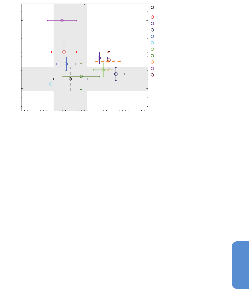
505
Carbon and Other Biogeochemical Cycles Chapter 6
6
−7 −5 −3 −1 1
−2
0
2
4
6
Sensitivity of Land CO
2
Sink Interannual Variations to
Temperature Interannual Variations (PgC yr
−1
o
C
−1
)
Sensitivity of Land CO
2
Sink Interannual Variations to
Precipitation Interannual Variations (PgC yr
−1
100 mm
−1
)
residual land sink
(see Fig 6.15 and Table 6.1)
CLM4C
CLM4CN
HYLAND
LPJ
LPJ−GUESS
OCN
ORCHIDEE
SDGVM
TRIFFID
VEGAS
Figure 6.17 | The response of interannual land CO
2
flux anomaly to per 1°C interannual temperature anomaly and per 100 mm interannual precipitation anomaly during
1980–2009. Black circles show climate sensitivity of land CO
2
sink estimated from the residual land sink (see Figure 6.15 and Table 6.1), which is the sum of fossil fuel and cement
emissions and land use change emissions minus the sum of observed atmospheric CO
2
growth rate and modeled ocean sink sink (Le Quéré et al., 2009; Friedlingstein and Prentice,
2010). Coloured circles show land CO
2
sink estimated by 10 process-based terrestrial carbon cycle models (CLM4C (Community Land Model for Carbon), CLM4CN (Community Land
Model for Carbon–Nitrogen), HYLAND (HYbrid LAND terrestrial ecosystem model), LPJ (Lund-Potsdam-Jena Dynamic Global Vegetation Model), LPJ–GUESS (LPJ–General Ecosystem
Simulator, OCN (Cycling of Carbon and Nitrogen on land, derived from ORCHIDEE model), ORCHIDEE (ORganizing Carbon and Hydrology in Dynamic EcosystEms model), SDGVM
(Sheffield Dynamic Global Vegetation Model), TRIFFID (Top-down Representation of Interactive Foliage and Flora Including Dynamics) and VEGAS (terrestrial vegetation and carbon
model)). Error bars show standard error of the sensitivity estimates. Dashed error bars indicate the estimated sensitivity by the regression approach is statistically insignificant (P >
0.05). Grey area denoted the area bounded by the estimated climate sensitivity of the residual land sink ± the standard error of the estimated climate sensitivity of the residual land
sink. The sensitivity of land CO
2
sink interannual variations to interannual variations of temperature (or precipitation) is estimated as the regression coefficient of temperature (or
precipitation) in a multiple regression of detrended anomaly of land CO
2
sink against detrended anomaly of annual mean temperature and annual precipitation.
6.3.3 Global Methane Budget
AR5 is the first IPCC assessment report providing a consistent synthesis
of the CH
4
budget per decade using multiple atmospheric CH
4
inver-
sion models (top-down) and process-based models and inventories
(bottom-up). Table 6.8 shows the budgets for the decades of 1980s,
1990s and 2000s. Uncertainties on emissions and sinks are listed using
minimum and maximum of each published estimate for each decade.
Bottom-up approaches are used to attribute decadal budgets to indi-
vidual processes emitting CH
4
(see Section 6.1.1.2 for a general over-
view). Top-down inversions provide an atmospheric-based constraint
mostly for the total CH
4
source per region, and the use of additional
observations (e.g., isotopes) allows inferring emissions per source type.
Estimates of CH
4
sinks in the troposphere by reaction with tropospheric
OH, in soils and in the stratosphere are also presented. Despite signif-
icant progress since the AR4, large uncertainties remain in the present
knowledge of the budget and its evolution over time.
6.3.3.1 Atmospheric Changes
Since the beginning of the Industrial Era, the atmospheric CH
4
concen-
tration increased by a factor of 2.5 (from 722 ppb to 1803 ppb in 2011).
CH
4
is currently measured by a network of more than 100 surface sites
(Blake et al., 1982; Cunnold et al., 2002; Langenfelds et al., 2002; Dlu-
gokencky et al., 2011), aircraft profiles (Brenninkmeijer et al., 2007),
satellite (Wecht et al., 2012; Worden et al., 2012) and before 1979 from
analyses of firn air and ice cores (see Sections 5.2.2 and Section 6.2,
and Figure 6.11). The growth of CH
4
in the atmosphere is largely in
response to increasing anthropogenic emissions. The vertically aver-
aged atmospheric CH
4
concentration field can be mapped by remote
sensing from the surface using Fourier Transform Infrared Spectroscopy
(FTIR) instruments (Total Carbon Column Observing Network, TCCON,
http://www.tccon.caltech.edu/) and from space by several satellite
instruments: Atmospheric Infrared Sounder (AIRS, since 2002; http://
airs.jpl.nasa.gov), Tropospheric Emission Spectrometer (TES, since
2004; http://tes.jpl.nasa.gov), Infrared Atmospheric Sounder Interfer-
ometer (IASI, since 2006; Crévoisier et al., 2009), Scanning Imaging
Spectrometer for Atmospheric Cartography (SCIAMACHY, 2003–2012;
Frankenberg et al., 2008), and Greenhouse Gases Observing Satel-
lite-Thermal And Near infrared Sensor for carbon Observation Fouri-
er-Transform Spectrometer (GOSAT-TANSO-FTS, since 2009; Morino et
al., 2011). As an example, SCIAMACHY shows the column CH
4
gradient
between the two hemispheres as well as increased concentrations over
Southeast Asia, due to emissions from agriculture, wetlands, waste and
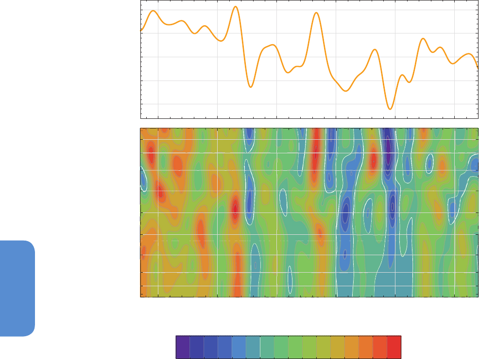
506
Chapter 6 Carbon and Other Biogeochemical Cycles
6
energy production (Frankenberg et al., 2008). In situ observations pro-
vide very precise measurements (~0.2%) but unevenly located at the
surface of the globe. Satellite data offer a global coverage at the cost
of a lower precision on individual measurements (~2%) and possible
biases (Bergamaschi et al., 2009).
The growth rate of CH
4
has declined since the mid-1980s, and a near
zero growth rate (quasi-stable concentrations) was observed during
1999–2006, suggesting an approach to steady state where the sum
of emissions are in balance with the sum of sinks (Dlugokencky et al.,
2003; Khalil et al., 2007; Patra et al., 2011; Figure 6.18). The reasons
for this growth rate decline after the mid-1980s are still debated, and
results from various studies provide possible scenarios: (1) a reduc-
tion of anthropogenic emitting activities such as coal mining, gas
industry and/or animal husbandry, especially in the countries of the
former Soviet Union (Dlugokencky et al., 2003; Chen and Prinn, 2006;
Savolainen et al., 2009; Simpson et al., 2012); (2) a compensation
between increasing anthropogenic emissions and decreasing wetland
emissions (Bousquet et al., 2006; Chen and Prinn, 2006); (3) significant
(Rigby et al., 2008) to small (Montzka et al., 2011) changes in OH con-
centrations and/or based on two different
13
CH
4
data sets; (4) reduced
emissions from rice paddies attributed to changes in agricultural prac-
tices (Kai et al., 2011); or (5) stable microbial and fossil fuel emissions
from 1990 to 2005 (Levin et al., 2012).
Since 2007, atmospheric CH
4
has been observed to increase again
(Rigby et al., 2008; Dlugokencky et al., 2009) with positive anoma-
lies of emissions of 21 Tg(CH
4
) yr
–1
and 18 Tg(CH
4
) yr
–1
estimated by
inversions during 2007 and 2008, respectively (Bousquet et al., 2011)
as compared to the 1999–2006 period. The increase of emissions in
2007–2008 was dominated by tropical regions (Bousquet et al., 2011),
with a major contribution from tropical wetlands and some contribu-
tion from high-latitude wetlands during the 2007 anomaly (Dlugo-
kencky et al., 2009; Bousquet et al., 2011). This increase is suggested by
the growth rate over latitude in Figure 6.18 (Dlugokencky et al., 2009).
The recent increase of CH
4
concentration since 2007 is also consistent
-5
0
5
10
15
1985 1990 1995 2000 2005 2010
ppb yr
-
1
(
)
1985 1990 1995 2000 2005 2010
90S
60S
45S
30S
15S
EQ
15N
30N
45N
60N
90N
Year
Latitude
-15 - 10 -5 0 5 10 15 20 25
ppb yr
-
1
(
)
Figure 6.18 | (Top) Globally averaged growth rate of atmospheric CH
4
in ppb yr
–1
determined from the National Oceanic and Atmospheric Administration–Earth System Research
Laboratory (NOAA–ESRL) network, representative for the marine boundary layer.(Bottom) Atmospheric growth rate of CH
4
as a function of latitude (Masarie and Tans, 1995;
Dlugokencky and Tans, 2013b).

507
Carbon and Other Biogeochemical Cycles Chapter 6
6
Tg(CH
4
) yr
–1
1980–1989 1990–1999 2000–2009
Top-Down Bottom-Up Top-Down Bottom-Up Top-Down Bottom-Up
Natural Sources 193 [150–267] 355 [244–466] 182 [167–197] 336 [230–465] 218 [179–273] 347 [238–484]
Natural wetlands 157 [115–231]
1,2,3
225 [183–266]
4,5
150 [144–160]
1,28,29
206 [169–265]
4,5,27
175 [142–
208]
1,29,33,34,35,36
217 [177–284]
4,5,27
Other sources 36 [35–36]
1,2
130 [61–200] 32 [23–37]
1,28,29
130 [61–200] 43 [37–65]
1,29,33,34,35,36
130 [61–200]
Freshwater (lakes and rivers) 40 [8–73]
6,7,8
40 [8–73]
6,7,8
40 [8–73]
6,7,8
Wild animals 15 [15–15]
9
15 [15–15]
9
15 [15–15]
9
Wildfires 3 [1–5]
9,10,11,12,13
3 [1–5]
9,10,11,12,13
3 [1–5]
9,10,11,12,13
Termites 11 [2–22]
9,10,14,15,x
11 [2–22]
9,10,14,15,x
11 [2–22]
9,10,14,15,x
Geological (incl. oceans) 54 [33–75]
10,16,17
54 [33–75]
10,16,17
54 [33–75]
10,16,17
Hydrates 6 [2–9]
9,18,19
6 [2–9]
9,18,19
6 [2–9]
9,18,19
Permafrost (excl. lakes
and wetlands)
1 [0–1]
10
1 [0–1]
10
1 [0–1]
10
Anthropogenic Sources 348 [305–383] 308 [292–323] 372 [290–453] 313 [281–347] 335 [273–409] 331 [304–368]
Agriculture and waste 208 [187–220]
1,2,3
185 [172–197]
20
239 [180–301]
1,28,29
187 [177–196]
20,30,31
209 [180–
241]
1,29,33,34,35,36
200 [187–224]
20,30,31
Rice 45 [41–47]
20
35 [32–37]
20,27,30,31
36 [33–40]
20,27,30,31
Ruminants 85 [81–90]
20
87 [82–91]
20,30,31
89 [87–94]
20,30,31
Landfills and waste 55 [50–60]
20
65 [63–68]
20,30,31
75 [67–90]
20,30,31
Biomass burning (incl. biofuels) 46 [43–55]
1,2,3
34 [31–37]
20,21,22a,38
38 [26–45]
1,28,29
42 [38–45]
13,20,21,22a,32,38
30 [24–45]
1,29,33,34,35,36
35 [32–39]
13,20,21,32,37,38
Fossil fuels 94 [75–108]
1,2,3
89 [89–89]
20
95 [84–107]
1,28,29
84 [66–96]
20,30,31
96 [77–
123]
1,29,33,34,35,36
96 [85–105]
20,30,31
Sinks
Total chemical loss 490 [450–533]
1,2,3
539 [411–671]
23,24,25,26
515 [491–554]
1,28,29
571 [521–621]
23,24,25,26
518 [510–
538]
1,29,33,34,36
604 [483–738]
23,24,25,26
Tropospheric OH 468 [382–567]
26
479 [457–501]
26
528 [454–617]
25,26
Stratospheric OH 46 [16–67]
23,25,26
67 [51–83]
23,25,26
51 [16–84]
23,25,26
Tropospheric Cl 25 [13–37]
24
25 [13–37]
24
25 [13–37]
24
Soils 21 [10–27]
1,2,3
28 [9–47]
27,34,36
27 [27–27]
1
28 [9–47]
27,34,36
32 [26–42]
1,33,34,35,36
28 [9–47]
27,34,36
Global
Sum of sources 541 [500–592] 663 [536–789] 554 [529–596] 649 [511–812] 553 [526–569] 678 [542–852]
Sum of sinks 511 [460–559] 567 [420–718] 542 [518–579] 599 [530–668] 550 [514–560] 632 [592–785]
Imbalance (sources
minus sinks)
30 [16–40] 12 [7–17] 3 [–4–19]
Atmospheric growth rate 34 17 6
Global top-down (year 2011) 2011 (AR5)
38
Burden (Tg CH
4
) 4954±10
Atmospheric loss (Tg CH
4
yr
-1
) 542±56
Atmos. increase (Tg CH
4
yr
-1
) 14±3
Total source (Tg CH
4
yr
-1
) 556±56
Anthropogenic source
(Tg CH
4
yr
-1
)
354±45
Natural source (Tg CH
4
yr
-1
) 202±35
References:
1
Bousquet et al. (2011)
2
Fung et al. (1991)
3
Hein et al. (1997)
4
Hodson et al. (2011)
5
Ringeval et al. (2011)
6
Bastviken et al. (2004)
7
Bastviken et al. (2011)
8
Walter et al. (2007)
9
Denman et al. (2007)
10
EPA (2010)
Table 6.8 | Global CH
4
budget for the past three decades (in Tg(CH
4
) yr
–1
) and present day (2011)
38
. The bottom-up estimates for the decade of 2000–2009 are used in the
Executive Summary and in Figure 6.2. T-D stands for Top-Down inversions and B-U for Bottom-Up approaches. Only studies covering at least 5 years of each decade have been
used. Reported values correspond to the mean of the cited references and therefore not always equal (max-min)/2; likewise, ranges [in brackets] represent minimum and maximum
values of the cited references. The sum of sources and sinks from B-U approaches does not automatically balance the atmospheric changes. For B-U studies, individual source
types are also presented. For T-D inversions, the 1980s decade starts in 1984. As some atmospheric inversions did not reference their global sink, balance with the atmosphere
and the sum of the sources has been assumed. One biomass burning estimate (Schultz et al., 2007) excludes biofuels (a). Stratospheric loss for B-U is the sum of the loss by OH
radicals, a 10 Tg yr
–1
loss due to O1D radicals (Neef et al., 2010) and a 20 to 35% contribution due to Cl radicals
24
(Allan et al., 2007). Present day budgets
39
adopt a global
mean lifetime of 9.14 yr (±10%).

508
Chapter 6 Carbon and Other Biogeochemical Cycles
6
with anthropogenic emission inventories, which show more (EDGAR
v4.2) or less (EPA, 2011a) rapidly increasing anthropogenic CH
4
emis-
sions in the period 2000–2008. This is related to increased energy
production in growing Asian economies (EDGAR, edgar.jrc.ec.europa.
eu; EPA, http://www.epa.gov/nonco2/econ-inv/international.html). The
atmospheric increase has continued after 2009, at a rate of 4 to 5 ppb
yr
–1
(Sussmann et al., 2012).
6.3.3.2 Methane Emissions
\The CH
4
growth rate results from the balance between emissions and
sinks. Methane emissions around the globe are biogenic, thermogenic
or pyrogenic in origin (Neef et al., 2010), and they can be the direct
result of either human activities and/or natural processes (see Section
6.1.1.2 and Table 6.8). Biogenic sources are due to degradation of
organic matter in anaerobic conditions (natural wetlands, ruminants,
waste, landfills, rice paddies, fresh waters, termites). Thermogenic
sources come from the slow transformation of organic matter into
fossil fuels on geological time scales (natural gas, coal, oil). Pyrogenic
sources are due to incomplete combustion of organic matter (biomass
and biofuel burning). Some sources can eventually combine a biogenic
and a thermogenic origin (e.g., natural geological sources such as oce-
anic seeps, mud volcanoes or hydrates). Each of these three types of
emissions is characterized by ranges in its isotopic composition in
13
C-
CH
4
: typically –55 to –70‰ for biogenic, –25 to –45‰ for thermogenic,
and –13 to –25‰ for pyrogenic. These isotopic distinctions provide a
basis for attempting to separate the relative contribution of different
methane sources using the top-down approach (Bousquet et al., 2006;
Neef et al., 2010; Monteil et al., 2011).
During the decade of the 2000s, natural sources of CH
4
account for 35
to 50% of the decadal mean global emissions (Table 6.8). The single
most dominant CH
4
source of the global flux and interannual variability
is CH
4
emissions from wetlands (177 to 284 Tg(CH
4
)
yr
–1
). With high
confidence, climate driven changes of emissions from wetlands are the
main drivers of the global inter-annual variability of CH
4
emissions.
The term ‘wetlands’ denotes here a variety of ecosystems emitting
CH
4
in the tropics and the high latitudes: wet soils, swamps, bogs and
peatlands. These emissions are highly sensitive to climate change and
variability, as shown, for instance, from the high CH
4
growth rate in
2007–2008 that coincides with positive precipitation and temperature
anomalies (Dlugokencky et al., 2009). Several process-based models of
methane emissions from wetlands have been developed and improved
since AR4 (Hodson et al., 2011; Ringeval et al., 2011; Spahni et al.,
2011; Melton et al., 2013), yet the confidence in modeled wetland
CH
4
emissions remains low, particularly because of limited observa-
tional data sets available for model calibration and evaluation. Spatial
distribution and temporal variability of wetlands also remains highly
unconstrained in spite the existence of some remote sensing products
(Papa et al., 2010). It has been observed that wetland CH
4
emissions
increase in response to elevated atmospheric CO
2
concentrations (van
Groenigen et al., 2011). van Groenigen et al. attribute such an increase
in CH
4
emissions from natural wetlands to increasing soil moisture due
to the reduced plant demand for water under higher CO
2
. However, the
sign and magnitude of the CH
4
emission response to changes in tem-
perature and precipitation vary among models but show, on average,
a decrease of wetland area and CH
4
flux with increasing temperature,
especially in the tropics, and a modest (~4%) increase of wetland area
and CH
4
flux with increasing precipitation (Melton et al., 2013).
In AR4, natural geological sources were estimated between 4 and 19
Tg(CH
4
) yr
–1
. Since then, Etiope et al. (2008) provided improved emis-
sion estimates from terrestrial (13 to 29 Tg(CH
4
) yr
–1
) and marine (~20
Tg(CH
4
) yr
–1
) seepages, mud volcanoes (6 to 9 Tg(CH
4
) yr
–1
), hydrates (5
to 10 Tg(CH
4
) yr
–1
) and geothermal and volcanic areas (3 to 6 Tg(CH
4
)
yr
–1
), which represent altogether between 42 and 64 Tg(CH
4
) yr
–1
(see
Table 6.8 for full range of estimates). This contribution from natural,
geological and partly fossil CH
4
is larger than in AR4 and consistent
with a
14
CH
4
reanalysis showing natural and anthropogenic fossil con-
tributions to the global CH
4
budget to be around 30% (medium confi-
dence) (Lassey et al., 2007) and not around 20% as previously estimat-
ed (e.g., AR4). However, such a large percentage was not confirmed by
an analysis of the global atmospheric record of ethane (Simpson et al.,
2012) which is co-emitted with geological CH
4
.
Of the natural sources of CH
4
, emissions from thawing permafrost and
CH
4
hydrates in the northern circumpolar region will become poten-
tially important in the 21st century because they could increase dra-
matically due to the rapid climate warming of the Arctic and the large
carbon pools stored there (Tarnocai et al., 2009; Walter Anthony et al.,
2012) (see Section 6.4.3.4). Hydrates are, however, estimated to rep-
resent only a very small emission, between 2 and 9 Tg(CH
4
) yr
–1
under
the current time period (Table 6.8). Supersaturation of dissolved CH
4
at
the bottom and surface waters in the East Siberian Arctic Shelf indicate
some CH
4
activity across the region, with a net sea–air flux of 10.5
Tg(CH
4
) yr
–1
which is similar in magnitude to the flux for the entire
ocean (Shakhova et al., 2010) but it is not possible to say whether this
source has always been present or is a consequence of recent Arctic
changes. The ebullition of CH
4
from decomposing, thawing lake sed-
iments in north Siberia with an estimated flux of ~4 Tg(CH
4
) yr
−1
is
another demonstration of the activity of this region and of its potential
importance in the future (Walter et al., 2006; van Huissteden et al.,
2011). The sum of all natural emission estimates other than wetlands
is still very uncertainbased on bottom-up studies [see Table 6.8, range
of 238 to 484 Tg(CH
4)
yr
–1
for 2000–2009].
Table 6.8 References (continued)
11
Hoelzemann et al. (2004)
12
Ito and Penner (2004)
13
van der Werf et al. (2010)
14
Sanderson (1996)
15
Sugimoto et al. (1998)
16
Etiope et al. (2008)
17
Rhee et al. (2009)
18
Dickens (2003)
19
Shakhova et al. (2010)
20
EDGAR4-database (2009)
21
Mieville et al. (2010)
22
Schultz et al. (2007)
(excluding biofuels)
23
Neef et al. (2010)
24
Allan et al. (2007)
25
Williams et al. (2012b)
26
Voulgarakis et al. (2013)
27
Spahni et al. (2011)
28
Chen and Prinn (2006)
29
Pison et al. (2009)
30
Dentener et al. (2005)
31
EPA (2011a)
32
van der Werf (2004)
33
Bergamaschi et al. (2009)
34
Curry (2007)
35
Spahni et al. (2011)
36
Ito and Inatomi (2012)
37
Wiedinmyer et al. (2011)
38
Andreae and Merlet (2001)
39
Prather et al. (2012), updated to
2011 (Table 2.1) and used in
Chapter 11 projections;
uncertainties evaluated as
68% confidence intervals, see
also Annex II.2.2 and II.4.2.

509
Carbon and Other Biogeochemical Cycles Chapter 6
6
Pyrogenic sources of CH
4
(biomass burning in Table 6.8) are assessed
to have a small contribution in the global flux for the 2000s (32 to
39 Tg(CH
4
) yr
−1
). Biomass burning of tropical and boreal forests (17 to
21 Tg(CH
4
) yr
−1
) play a much smaller role than wetlands in interannual
variability of emissions, except during intensive fire periods (Langen-
felds et al., 2002; Simpson et al., 2006). Only during the 1997–1998
record strong El Niño, burning of forests and peatland that took place
in Indonesia and Malaysia, released ~12 Tg(CH
4
) and contributed to the
observed growth rate anomaly
(Langenfelds et al., 2002; van der Werf
et al., 2004). Other smaller fire CH
4
emissions positive anomalies were
suggested over the northern mid-latitudes in 2002–2003, in particular
over Eastern Siberia in 2003 (van der Werf et al., 2010) and Russia in
2010. Traditional biofuel burning is estimated to be a source of 14 to 17
Tg(CH
4
) yr
–1
(Andreae and Merlet, 2001; Yevich and Logan, 2003).
Keppler at al. (2006) reported that plants under aerobic conditions
were able to emit CH
4
, and thus potentially could constitute a large
additional emission, which had not been previously considered in the
global CH
4
budget. Later studies do not support plant emissions as a
widespread mechanism (Dueck et al., 2007; Wang et al., 2008; Nisbet
et al., 2009) or show small to negligible emissions in the context of
the global CH
4
budget (Vigano et al., 2008; Nisbet et al., 2009; Bloom
et al., 2010). Alternative mechanisms have been suggested to explain
an apparent aerobic CH
4
production, which involve (1) adsorption
and desorption (Kirschbaum and Walcroft, 2008; Nisbet et al., 2009),
(2) degradation of organic matter under strong ultraviolet (UV) light
(Dueck et al., 2007; Nisbet et al., 2009) and (3) methane in the ground-
water emitted through internal air spaces in tree bodies (Terazawa
et al., 2007). Overall, a significant emission of CH
4
by plants under
aerobic conditions is very unlikely, and this source is not reported in
Table 6.8.
Anthropogenic CH
4
sources are estimated to range between 50% and
65% of the global emissions for the 2000s (Table 6.8). They include
rice paddies agriculture, ruminant animals, sewage and waste, land-
fills, and fossil fuel extraction, storage, transformation, transportation
and use (coal mining, gas and oil industries). Anthropogenic sources
are dominant over natural sources in top-down inversions (~65%) but
they are of the same magnitude in bottom-up models and inventories
(Table 6.8). Rice paddies emit between 33 to 40 Tg(CH
4
) yr
–1
and 90%
of these emissions come from tropical Asia, with more than 50% from
China and India (Yan et al., 2009). Ruminant livestock, such as cattle,
sheep, goats, etc. produce CH
4
by food fermentation in their anoxic
rumens with a total estimate of between 87 and 94 Tg(CH
4
) yr
–1
. Major
regional contributions of this flux come from India, China, Brazil and
the USA (EPA, 2006; Olivier and Janssens-Maenhout, 2012), EDGAR
v4.2. India, with the world’s largest livestock population emitted 11.8
Tg(CH
4
) yr
–1
in 2003, including emission from enteric fermentation
(10.7 Tg(CH
4
) yr
–1
) and manure management (1.1 Tg(CH
4
) yr
–1
; Chhabra
et al., 2013). Methanogenesis in landfills, livestock manure and waste
waters produces between 67 and 90 Tg(CH
4
) yr
–1
due to anoxic con-
ditions and a high availability of acetate, CO
2
and H
2
. Loss of natural
gas (~90% CH
4
) is the largest contributor to fossil fuel related fugitive
emissions, estimated between 85 and 105 Tg(CH
4
) yr
–1
in the USA (EPA,
2006; Olivier and Janssens-Maenhout, 2012), EDGAR v4.2.
6.3.3.3 Sinks of Atmospheric Methane
The main sink of atmospheric CH
4
is its oxidation by OH radicals, a
chemical reaction that takes place mostly in the troposphere and strat-
osphere (Table 6.8). OH removes each year an amount of CH
4
equiva-
lent to 90% of all surface emissions (Table 6.8), that is, 9% of the total
burden of CH
4
in the atmosphere, which defines a partial atmospheric
lifetime with respect to OH of 7 to 11 years for an atmospheric burden
of 4800 Tg(CH
4
) (4700 to 4900 TgCH
4
as computed by Atmospheric
Chemistry and Climate Model Intercomparison Project (ACCMIP)
atmospheric chemistry models in Voulgarakis et al. (2013), thus slightly
different from Figure 6.2; see Section 8.2.3.3 for ACCMIP models). A
recent estimate of the CH
4
lifetime is 9.1 ± 0.9 years (Prather et al.,
2012). A small sink of atmospheric CH
4
is suspected, but still debated,
in the marine boundary layer due to a chemical reaction with chlorine
(Allan et al., 2007). Another small sink is the reaction of CH
4
with Cl
radicals and O(1D) in the stratosphere (Shallcross et al., 2007; Neef
et al., 2010). Finally, oxidation in upland soils (with oxygen) by meth-
anotrophic bacterias removes about 9 to 47 Tg(CH
4
) yr
–1
(Curry, 2007;
Dutaur and Verchot, 2007; Spahni et al., 2011; Ito and Inatomi, 2012).
There have been a number of published estimates of global OH con-
centrations and variations over the past decade (Prinn et al., 2001;
Dentener et al., 2003; Bousquet et al., 2005; Prinn et al., 2005; Rigby
et al., 2008; Montzka et al., 2011). The very short lifetime of OH makes
it almost impossible to measure directly global OH concentrations in
the atmosphere. Chemistry transport models (CTMs), chemistry climate
models (CCMs) or proxy methods have to be used to obtain a global
mean value and time variations. For the 2000s, CTMs and CCMs (Young
et al., 2013) estimate a global chemical loss of methane due to OH
of 604 Tg(CH
4
) yr
–1
(509 to 764 Tg(CH
4
) yr
–1
). This loss is larger, albeit
compatible considering the large uncertainties, with a recent exten-
sive analysis by Prather et al. (2012) inferring a global chemical loss of
554 ± 56 Tg(CH
4
) yr
–1
. Top-down inversions using methyl-chloroform
(MCF) measurements to infer OH provide a smaller chemical loss of
518 Tg(CH
4
) yr
–1
with a more narrow range of 510 to 538 Tg(CH
4
) yr
–1
in the 2000s. However, inversion estimates probably do not account for
all sources of uncertainties (Prather et al., 2012).
CCMs and CTMs simulate small interannual variations of OH radicals,
typically of 1 to 3% (standard deviation over a decade) due to a high
buffering of this radical by atmospheric photochemical reactions (Voul-
garakis et al., 2013; Young et al., 2013). Atmospheric inversions show
much larger variations for the 1980s and the 1990s (5 to 10%), because
of their oversensitivity to uncertainties on MCF emissions, when meas-
urements of this tracer are used to reconstruct OH (Montzka et al.,
2011), although reduced variations are inferred after 1998 by Prinn et
al. (2005). For the 2000s, the reduction of MCF in the atmosphere, due
to the Montreal protocol (1987) and its further amendments, allows
a consistent estimate of small OH variations between atmospheric
inversions (<±5%) and CCMs/CTMs (<±3%). However, the very low
atmospheric values reached by MCF (few ppt in 2010) impose the
need to find another tracer to reconstruct global OH in the upcoming
years. Finally, evidence for the role of changes in OH concentrations in
explaining the increase in atmospheric methane since 2007 is variable,
ranging from a significant contribution (Rigby et al., 2008) to only a
small role (Bousquet et al., 2011).

510
Chapter 6 Carbon and Other Biogeochemical Cycles
6
6.3.3.4 Global Methane Budget for the 2000s
Based on the inversion of atmospheric measurements of CH
4
from sur-
face stations, global CH
4
emissions for the 2000s are of 553 Tg(CH
4
)
yr
–1
, with a range of 526 to 569 Tg(CH
4
) yr
–1
(Table 6.8). The total loss of
atmospheric methane is of 550 Tg(CH
4
) yr
–1
with a range of 514 to 560
Tg(CH
4
) yr
–1
, determining a small imbalance of about 3Tg(CH
4
) yr
–1
, in
line with the small growth rate of 6 Tg(CH
4
) yr
–1
observed for the 2000s.
Based on bottom-up models and inventories, a larger global CH
4
emis-
sions of 678 Tg(CH
4
)
yr
–1
are found, mostly because of the still debated
upward re-evaluation of geological (Etiope et al., 2008) and freshwa-
ter (Walter et al., 2007; Bastviken et al., 2011) emission sources. An
averaged total loss of 632 Tg(CH
4
) yr
–1
is found, by an ensemble of
Atmospheric Chemistry models (Lamarque et al., 2013) leading to an
imbalance of about 45 Tg(CH
4
) yr
–1
during the 2000s, as compared
to the observed mean growth rate of 6 Tg(CH
4
) yr
–1
(Table 6.8; Dlugo-
kencky et al., 2011). There is no constraint that applies to the sum of
emissions in the bottom-up approach, unlike for top-down inversions
when these have constrained OH fields (e.g., from MCF). Therefore,
top-down inversions can help constrain global CH
4
emissions in the
global budget, although they do not resolve the same level of detail in
the mix of sources than the bottom-up approaches, and thus provide
more limited information about processes (Table 6.8).
6.3.4 Global Nitrogen Budgets and Global Nitrous
Oxide Budget in the 1990s
The atmospheric abundance of N
2
O has been increasing mainly as a
result of agricultural intensification to meet the food demand for a
growing human population. Use of synthetic fertiliser (primarily from
the Haber–Bosch process) and manure applications increase the pro-
duction of N
2
O in soils and sediments, via nitrification and denitrifica-
tion pathways, leading to increased N
2
O emissions to the atmosphere.
Increased emissions occur not only in agricultural fields, but also in
aquatic systems after nitrogen leaching and runoff, and in natural
soils and ocean surface waters as a result of atmospheric deposition
of nitrogen originating from agriculture, fossil fuel combustion and
industrial activities. Food production is likely responsible for 80% of
the increase in atmospheric N
2
O (Kroeze et al., 1999; Davidson, 2009;
Williams and Crutzen, 2010; Syakila and Kroeze, 2011; Zaehle et al.,
2011; Park et al., 2012), via the addition of nitrogen fertilisers. Global
emissions of N
2
O are difficult to estimate owing to heterogeneity in
space and time. Table 6.9 presents global emissions based on upscaling
of local flux measurements at the surface. Modelling of the atmos-
pheric lifetime of N
2
O and atmospheric inversions constrain global and
regional N
2
O budgets (Hirsch et al., 2006; Huang et al., 2008; Rhee et
al., 2009; Prather et al., 2012), although there is uncertainty in these
estimates because of uncertainty in the dominant loss term of N
2
O,
that is, the destruction of N
2
O by photolysis and reaction with O(1D)
in the stratosphere. The long atmospheric lifetime of N
2
O (118 to 131
years, Volk et al., 1997; Hsu and Prather, 2010; Fleming et al., 2011; see
Chapter 8) implies that it will take more than a century before atmos-
pheric abundances stabilise after the stabilization of global emissions.
This is of concern not only because of its contribution to the radiative
forcing (see Glossary), but also because of the relative importance of
N
2
O and other GHGs in affecting the ozone layer (Ravishankara et al.,
2009; Fleming et al., 2011).
Since AR4 (Table 6.9 for the 1990s), a number of studies allow us to
update some of the N
2
O emission estimates. First and most important-
ly, the IPCC Guidelines were revised in 2006 (De Klein et al., 2007) and
in particular emission factors for estimating agricultural N
2
O emissions.
Applying these 2006 emission factors to global agricultural statistics
results in higher direct emissions from agriculture (from fertilised soils
and animal production) than in AR4, but into indirect emissions (asso-
ciated with leaching and runoff of Nr resulting in N
2
O emissions from
groundwater, riparian zones and surface waters) that are considerably
lower than reported in AR4 (Table 6.9). It should be noted that emis-
sions of N
2
O show large uncertainties when default emission factors
are applied at the global scale (Crutzen et al., 2008; Davidson, 2009;
Smith et al., 2012). Second, estimates of the anthropogenic source of
N
2
O from the open ocean have been made for the first time. These
emissions result from atmospheric deposition of anthropogenic Nr
(nitrogen oxides and ammonia/ammonium) (Duce et al., 2008; Sun-
tharalingam et al., 2012). This anthropogenic ocean N
2
O source was
implicitly included as part of the natural ocean N
2
O source in AR4, but
is now given as a separate anthropogenic source of 0.2 (0.1 to 0.4)
TgN yr
–1
in Table 6.9. Finally, a first estimate of global N
2
O uptake at
the surface is now available (Syakila et al., 2010; Syakila and Kroeze,
2011), based on reviews of measurements of N
2
O uptake in soils and
sediments (Chapuis-Lardy et al., 2007; Kroeze et al., 2007). The uncer-
tainty in this sink of N
2
O is large. On the global scale, this surface sink
is negligible, but at the local scale it may not be irrelevant.
6.3.4.1 Atmosphere Nitrous Oxide Burden and Growth Rate
The concentration of N
2
O is currently 20% higher than pre-industrial
levels (Figure 6.11; MacFarling-Meure et al., 2006). Figure 6.19 shows
the annual growth rate of atmospheric N
2
O estimated from direct
measurements (National Oceanic and Atmospheric Administration –
Global Monitoring Division (NOAA–GMD) network of surface stations).
On decadal time scales, the concentration of N
2
O has been increasing
at a rate of 0.73 ± 0.03 ppb yr
–1
. The interannual variability in mid- to
high-latitude N
2
O abundance in both the NH and SH was found to cor-
relate with the strength of the stratospheric Brewer–Dobson circula-
tion (Nevison et al., 2011). Variability in stratosphere to troposphere air
mass exchange, coupled with the stratospheric N
2
O sink is likely to be
responsible for a fraction of the interannual variability in tropospheric
N
2
O, but the understanding of this process is poor (Huang et al., 2008).
This removal process signal is obscured in the SH by the timing of oce-
anic thermal and biological ventilation signals (Nevison et al., 2011)
and terrestrial sources (Ishijima et al., 2009). These two factors may
thus also be important determinants of seasonal and interannual vari-
ability of N
2
O in the atmosphere. Quantitative understanding of terres-
trial N
2
O emissions variability is poor, although emissions are known
to be sensitive to soil water content (Ishijima et al., 2009). A first pro-
cess model-based estimate suggests that the mainly climate-driven
variability in the terrestrial source may account for only 0.07 ppb yr
–1
variability in atmospheric N
2
O growth rate, which would be difficult to
detect in the observed growth rate (Zaehle et al., 2011).
Most N
2
O is produced by biological (microbial) processes such as nitri-
fication and denitrification in terrestrial and aquatic systems, including
rivers, estuaries, coastal seas and the open ocean (Table 6.9; Freing et
al., 2012). In general, more N
2
O is formed when more reactive nitrogen

511
Carbon and Other Biogeochemical Cycles Chapter 6
6
Table 6.9 | Section 1 gives the global nitrogen budget (TgN yr
–1
): (a) creation of reactive nitrogen, (b) emissions of NO
x
, NH
3
in 2000s to atmosphere, (c) deposition of nitrogen to
continents and oceans, (d) discharge of total nitrogen to coastal ocean and (e) conversion of Nr to N
2
by denitrification. Section 2 gives the N
2
O budget for the year 2006, and for
the 1990s compared to AR4. Unit: Tg(N
2
O-N) yr
–1
.
SECTION 1 (NO
y
and NH
x
)
a. Conversion of N
2
to Nr 2005 2005 References
Anthropogenic sources
Fossil fuel combustion 30 (27–33) Fowler et al. (2013)
Haber–Bosch process
Fertiliser 100 (95–100) Galloway et al. (2008), Fowler et al. (2013)
Industrial feedstock 24 (22–26) Galloway et al. (2008), Fowler et al. (2013)
Biological nitrogen fixation (BNF) 60 (50–70) Herridge et al. (2008)
Anthropogenic total 210
Natural sources
BNF, terrestrial 58 (50–100) Vitousek et al. (2013)
BNF, marine 160 (140–177) Voss et al. (2013), Codispoti (2007)
Lightning 4 (3–5) AR4
Natural total 220
Total conversion of N
2
to reactive N 440
b. Emissions to Atmosphere
NO
x
NH
3
Fossil fuel combustion industrial processes 28.3 0.5 Dentener et al. (2006)
Agriculture 3.7 30.4 Dentener et al. (2006)
Biomass and biofuel burning 5.5 9.2 Dentener et al. (2006)
Anthropogenic total 37.5 40.1
Natural sources
Soils under natural vegetation 7.3 (5–8) 2.4 (1–10) AR4
Oceans —
8.2
(3.6)
AR4
Lightning 4 (3–5) — AR4
Natural total 11.3 10.6 AR4
Total sources 48.8 50.7
c. Deposition from the Atmosphere
NO
y
NH
x
Continents 27.1 36.1 Lamarque et al. (2010)
Oceans 19.8 17.0 Lamarque et al. (2010)
Total 46.9 53.1
d. Discharge to Coastal Ocean
Surface water N flux 45 Mayorga et al. (2010), Seitzinger et al. (2010)
e. Conversion of Nr to N
2
by Denitrification
Continents 109 (101–118) Bouwman et al. (2013)
(continued on next page)
is available. The production of N
2
O shows large spatial and temporal
variability. Emission estimates for tropical regions and for aquatic sys-
tems are relatively uncertain. Inverse modelling studies show that the
errors in emissions are large, especially in (sub)-tropical regions (e.g.,
Hirsch et al., 2006; Huang et al., 2008). Emissions from rivers, estuar-
ies and continental shelves have been the subject of debate for many
years (Seitzinger and Kroeze, 1998; De Klein et al., 2007). Recent stud-
ies confirm that rivers can be important sources of N
2
O, which could
be a reason to reconsider recent estimates of aquatic N
2
O emissions
(Beaulieu et al., 2011; Rosamond et al., 2012).
Table 6.9 does not include the formation of atmospheric N
2
O from
abiotic decomposition of ammonium nitrate in the presence of light,
appropriate relative humidity and a surface. This process recently has
been proposed as a potentially important source of N
2
O ( Rubasinghege
et al., 2011); however, a global estimate does not yet exist. Table 6.9
indicates that the global N
2
O emissions in the mid-1990s amount to
17.5 (8.1 to 30.7) TgN (N
2
O) yr
–1
. The uncertainty range is consistent
with that of atmospheric inversions studies (14.1 to 17.8) by Huang et
al. (2008). The estimates of anthropogenic N
2
O emissions of Table 6.9
are in line with the top-down estimates by Prather et al. (2012) of 6.5
± 1.3 TgN (N
2
O) yr
–1
, and somewhat higher than their estimates for

512
Chapter 6 Carbon and Other Biogeochemical Cycles
6
SECTION 2 (N
2
O)
AR5 (2006/2011) AR5 (mid-1990s) AR4 (1990s)
Anthropogenic sources
Fossil fuel combustion and industrial processes 0.7 (0.2–1.8)
a
0.7 (0.2–1.8)
a
0.7 (0.2–1.8)
Agriculture 4.1 (1.7–4.8)
b
3.7 (1.7–4.8)
b
2.8(1.7–4.8)
Biomass and biofuel burning 0.7(0.2–1.0)
a
0.7(0.2–1.0)
a
0.7(0.2–1.0)
Human excreta 0.2 (0.1–0.3)
a
0.2 (0.1–0.3)
a
0.2 (0.1–0.3)
Rivers, estuaries, coastal zones 0.6 (0.1–2.9)
c
0.6 (0.1–2.9)
c
1.7(0.5–2.9)
Atmospheric deposition on land 0.4 (0.3–0.9)
d
0.4 (0.3–0.9)
d
0.6 (0.3–0.9)
Atmospheric deposition on ocean 0.2 (0.1–0.4)
e
0.2 (0.1–0.4)
e
—
Surface sink –0.01 (0– -1)
f
–0.01 (0– -1)
f
—
Total anthropogenic sources 6.9 (2.7–11.1) 6.5 (2.7–11.1) 6.7 (2.7–11.1)
Natural sources
a
Soils under natural vegetation 6.6 (3.3–9.0) 6.6 (3.3–9.0) 6.6 (3.3–9.0)
Oceans 3.8(1.8–9.4) 3.8(1.8–9.4) 3.8(1.8–5.8)
Lightning — — —
Atmospheric chemistry 0.6 (0.3–1.2) 0.6 (0.3–1.2) 0.6 (0.3–1.2)
Total naturalsources 11.0 (5.4–19.6) 11.0 (5.4–19.6) 11.0 (5.4–19.6)
Total natural + anthropogenic sources 17.9 (8.1–30.7) 17.5 (8.1–30.7) 17.7 (8.5–27.7)
Stratospheric sink 14.3 (4.3–27.2)
g
Observed growth rate 3.61 (3.5–3.8)
h
Global top-down (year 2011)
i
Burden (Tg N) 1553
Atmospheric Loss 11.9±0.9
Atmospheric Increase 4.0±0.5
Total Source 15.8±1.0
Natural Source 9.1±1.0
Anthropogenic Source 6.7±1.3
Notes:
a
All units for N
2
O fluxes are in TgN (N
2
O) yr
–1
as in AR4 (not based on 2006 IPCC Guidelines). Lower end of range in the natural ocean from Rhee et al. (2009); higher end of the range from Bianchi
et al. (2012) and Olivier and Janssens-Maenhout (2012); natural soils in line with Stocker et al. (2013).
b
Direct soil emissions and emissions from animal production; calculated following 2006 IPCC Guidelines (Syakila and Kroeze, 2011); range from AR4 (Olivier and Janssens-Maenhout, 2012).
c
Following 2006 IPCC Guidelines (Kroeze et al., 2010; Syakila and Kroeze, 2011). Higher end of range from AR4; lower end of range from 1996 IPCC Guidelines (Mosier et al., 1998). Note that a
recent study indicates that emissions from rivers may be underestimated in the IPCC assessments (Beaulieu et al., 2011).
d
Following 2006 IPCC Guidelines (Syakila and Kroeze, 2011).
e
Suntharalingam et al. (2012).
f
Syakila et al. (2010).
g
The stratospheric sink regroups losses via photolysis and reaction with O(1D) that account for 90% and 10% of the sink, respectively (Minschwaner et al., 1993). The global magnitude of the
stratospheric sink was adjusted in order to be equal to the difference between the total sources and the observed growth rate. This value falls within literature estimates (Volk et al., 1997).
h
Data from Sections 6.1 and 6.3 (see Figure 6.4c). The range on the observed growth rate in this table is given by the 90% confidence interval of Figure 6.4c.
i
Based on Prather et al. (2012), updated to 2011 (Table 2.1) and used in Chapter 11 projections; uncertainties evaluated as 68% confidence intervals, N
2
O budget reduced based on recently
published longer lifetimes of 131±10 yrs, see Annex II.2.3 and II.4.3.
Table 6.9 (continued)
natural (9.1 ± 1.3 TgN (N
2
O) yr
–1
) and total (15.7 ± 1.1 TgN (N
2
O) yr
–1
)
emissions. Anthropogenic emissions have steadily increased over the
last two decades and were 6.9 (2.7 to 11.1) TgN (N
2
O) yr
–1
in 2006,
or 6% higher than the value in mid-1990s (Davidson, 2009; Zaehle et
al., 2011) (see also Figure 6.4c). Overall, anthropogenic N
2
O emissions
are now a factor of 8 greater than their estimated level in 1900. These
trends are consistent with observed increases in atmospheric N
2
O
(Syakila et al., 2010). Human activities strongly influence the source of
N
2
O, as nitrogen fertiliser used in agriculture is now the main source
of nitrogen for nitrification and denitrification (Opdyke et al., 2009).
Nitrogen stable isotope ratios confirm that fertilised soils are primar-
ily responsible for the historic increase in N
2
O (Röckmann and Levin,
2005; Sutka et al., 2006; Park et al., 2012).
6.3.4.2 Sensitivity of Nitrous Oxide Fluxes to Climate and
Elevated Carbon Dioxide
Previous studies suggested a considerable positive feedback between
N
2
O and climate (Khalil and Rasmussen, 1989) supported by observed
glacial–interglacial increases of ~70 ppb in atmospheric N
2
O (Flück-
iger et al., 1999). Climate change influences marine and terrestrial N
2
O
sources, but their individual contribution and even the sign of their
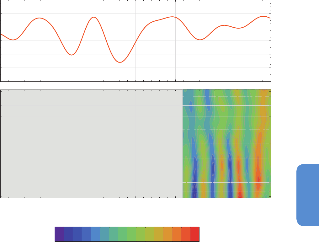
513
Carbon and Other Biogeochemical Cycles Chapter 6
6
Figure 6.19 | (Top) Globally averaged growth rate of atmospheric N
2
Oin ppb yr
–1
representative for the marine boundary layer. (Bottom) Atmospheric growth rate of N
2
Oas a
function of latitude.Sufficient observations are available only since the year 2002.Observations from the National Oceanic and Atmospheric Administration–Earth System Research
Laboratory (NOAA–ESRL) network(Masarie and Tans, 1995; Dlugokencky and Tans, 2013b).
0.0
0.2
0.4
0.6
0.8
1.0
1.2
1980 1990 2000 2010
0.0 0.5 1.0 1.5
ppb yr
-
1
(
)
ppb yr
-
1
(
)
1980 1985 1990 1995 2000 2005 2010
90S
60S
45S
30S
15S
EQ
15N
30N
45N
60N
90N
Year
Latitude
response to long-term climate variations are difficult to estimate (see
Section 6.2). Simulations by terrestrial biosphere models suggest a
moderate increase of global N
2
O emissions with recent climate chang-
es, related mainly to changes in land temperature (Zaehle and Dal-
monech, 2011; Xu-Ri et al., 2012), thus suggesting a possible posi-
tive feedback to the climate system. Nonetheless, the recent change
in atmospheric N
2
O is largely dominated to anthropogenic reactive
nitrogen (Nr) and industrial emissions (Holland et al., 2005; David-
son, 2009; Zaehle and Dalmonech, 2011). Stocker et al. (2013) have
found, using a global coupled model of climate and biogeochemical
cycles, that future climate change will amplify terrestrial N
2
O emissions
resulting from anthropogenic Nr additions, consistent with empirical
understanding (Butterbach-Bahl and Dannenmann, 2011). This result
suggests that the use of constant emission factors might underesti-
mate future N
2
O emission trajectories. Significant uncertainty remains
in the N
2
O–climate feedback from land ecosystems, given the poorly
known response of emission processes to the changes in seasonal and
frequency distribution of precipitation, and also because agricultural
emissions themselves may also be sensitive to climate.
N
2
O production will be affected by climate change through the effects
on the microbial nitrification and denitrification processes (Barnard et
al., 2005; Singh et al., 2010; Butterbach-Bahl and Dannenmann, 2011).
Warming experiments tend to show enhanced N
2
O emission (Lohila et
al., 2010; Brown et al., 2011; Chantarel et al., 2011; Larsen et al., 2011).
Elevated CO
2
predominantly increases N
2
O emissions(van Groenigen et
al., 2011); however, reductions have also been observed (Billings et al.,
2002; Mosier et al., 2002), induced by changes in soil moisture, plant
productivity and nitrogen uptake, as well as activity and composition
of soil microbial and fungal communities (Barnard et al., 2005; Singh
et al., 2010). The effect of interacting climate and atmospheric CO
2
change modulates and potentially dampens the individual responses
to each driver (Brown et al., 2011). A terrestrial biosphere model that
integrates the interacting effects of temperature, moisture and CO
2

514
Chapter 6 Carbon and Other Biogeochemical Cycles
6
changes is capable of qualitatively reproducing the observed sensitivi-
ties to these factors and their combinations (Xu-Ri et al., 2012). Thaw-
ing permafrost soils under particular hydrological settings may liberate
reactive nitrogen and turn into significant sources of N
2
O; however,
the global significance of this source is not established (Elberling et
al., 2010).
6.3.4.3 Global Nitrogen Budget
For base year 2010, anthropogenic activities created ~210 (190 to 230)
TgN of reactive nitrogen Nr from N
2
. This human-caused creation of
reactive nitrogen in 2010 is at least 2 times larger than the rate of nat-
ural terrestrial creation of ~58 TgN (50 to 100 TgN yr
–1
) (Table 6.9, Sec-
tion 1a). Note that the estimate of natural terrestrial biological fixation
(58 TgN yr
–1
) is lower than former estimates (100 TgN yr
–1
, Galloway
et al., 2004), but the ranges overlap, 50 to 100 TgN yr
–1
, vs. 90 to 120
TgN yr
–1
, respectively). Of this created reactive nitrogen, NO
x
and NH
3
emissions from anthropogenic sources are about fourfold greater than
natural emissions (Table 6.9, Section 1b). A greater portion of the NH
3
emissions is deposited to the continents rather than to the oceans, rel-
ative to the deposition of NO
y
, due to the longer atmospheric residence
time of the latter. These deposition estimates are lower limits, as they
do not include organic nitrogen species. New model and measurement
information (Kanakidou et al., 2012) suggests that incomplete inclu-
sion of emissions and atmospheric chemistry of reduced and oxidized
organic nitrogen components in current models may lead to system-
atic underestimates of total global reactive nitrogen deposition by up
to 35% (Table 6.9, Section 1c). Discharge of reactive nitrogen to the
coastal oceans is ~45 TgN yr
–1
(Table 6.9, Section 1d). Denitrification
converts Nr back to atmospheric N
2
. The current estimate for the pro-
duction of atmospheric N
2
is 110 TgN yr
–1
(Bouwman et al., 2013). Thus
of the ~280 TgN yr
–1
of Nr from anthropogenic and natural sources,
~40% gets converted to N
2
each year. The remaining 60% is stored in
terrestrial ecosystems, transported by rivers and by atmospheric trans-
port and deposition to the ocean, or emitted as N
2
O (a small fraction of
total Nr only despite the important forcing of increasing N
2
O emissions
for climate change). For the oceans, denitrification producing atmos-
pheric N
2
is 200 to 400 TgN yr
–1
, which is larger than the current uptake
of atmospheric N
2
by ocean biological fixation of 140 to 177 TgN yr
–1
(Table 6.9 Section 1e; Figure 6.4a).
6.4 Projections of Future Carbon and Other
Biogeochemical Cycles
6.4.1 Introduction
In this section, we assess coupled model projections of changes in the
evolution of CO
2
, CH
4
and N
2
O fluxes, and hence the role of carbon and
other biogeochemical cycles in future climate under socioeconomic
emission scenarios (see Box 6.4). AR4 reported how climate change
can affect the natural carbon cycle in a way that could feed back
onto climate itself. A comparison of 11 coupled climate–carbon cycle
models of different complexity (Coupled Carbon Cycle Climate–Model
Intercomparison Project (C4MIP); Friedlingstein et al., 2006) showed
that all 11 models simulated a positive feedback. There is substantial
quantitative uncertainty in future CO
2
and temperature, both across
coupled carbon–climate models (Friedlingstein et al., 2006; Plattner et
al., 2008) and within each model parametrizations (Falloon et al., 2011;
Booth et al., 2012; Higgins and Harte, 2012). This uncertainty on the
coupling between carbon cycle and climate is of comparable magni-
tude to the uncertainty caused by physical climate processes discussed
in Chapter 12 of this Report (Denman et al., 2007; Gregory et al., 2009;
Huntingford et al., 2009).
Other biogeochemical cycles and feedbacks play an important role in
the future of the climate system, although the carbon cycle represents
the strongest of these. Natural CH
4
emissions from wetland and fires
are sensitive to climate change (Sections 6.2, 6.4.7 and 6.3.3.2). The
fertilising effects of nitrogen deposition and rising CO
2
also affect CH
4
emissions by wetlands through increased plant productivity (Stocker
et al., 2013). Changes in the nitrogen cycle, in addition to interactions
with CO
2
sources and sinks, are very likely to affect the emissions of
N
2
O both on land and from the ocean (Sections 6.3.4.2 and 6.4.6)
and potentially on the rate of CH
4
oxidation (Gärdenäs et al., 2011). A
recent review highlighted the complexity of terrestrial biogeochemical
feedbacks on climate change (Arneth et al., 2010) and used the meth-
odology of Gregory et al. (2009) to express their magnitude in common
units of W m
–2
°C
–1
(Figure 6.20). A similar degree of complexity exists
in the ocean and in interactions between land, atmosphere and ocean
cycles. Many of these processes are not yet represented in coupled
climate–biogeochemistry models. Leuzinger et al. (2011) observed a
trend from manipulation experiments for higher-order interactions
between feedbacks to reduce the magnitude of response. Confidence
in the magnitude, and sometimes even the sign, of many of these feed-
backs between climate and carbon and other biogeochemical cycles
is low.
The response of land and ocean carbon storage to changes in climate,
atmospheric CO
2
and other anthropogenic activities (e.g., land use
change; Table 6.2) varies strongly on different time scales. This chapter
has assessed carbon cycle changes across many time scales from mil-
lennial (see Section 6.2) to interannual and seasonal (see Section 6.3),
and these are summarized in Table 6.10. A common result is that an
increase in atmospheric CO
2
will always lead to an increase in land and
ocean carbon storage, all other things being held constant. Cox et al.
(2013) find an empirical relationship between short-term interannual
variability and long-term land tropical carbon cycle sensitivity that may
offer an observational constraint on the climate–carbon cycle response
over the next century. Generally, however, changes in climate on dif-
ferent time scales do not lead to a consistent sign and magnitude of
the response in carbon storage change owing to the many different
mechanisms that operate. Thus, changes in carbon cycling on one time
scale cannot be extrapolated to make projections on different time
scales, but can provide valuable information on the processes at work
and can be used to evaluate and improve models.
6.4.2 Carbon Cycle Feedbacks in Climate Modelling
Intercomparison Project Phase 5 Models
6.4.2.1 Global Analysis
The carbon cycle response to future climate and CO
2
changes can be
viewed as two strong and opposing feedbacks (Gregory et al., 2009).
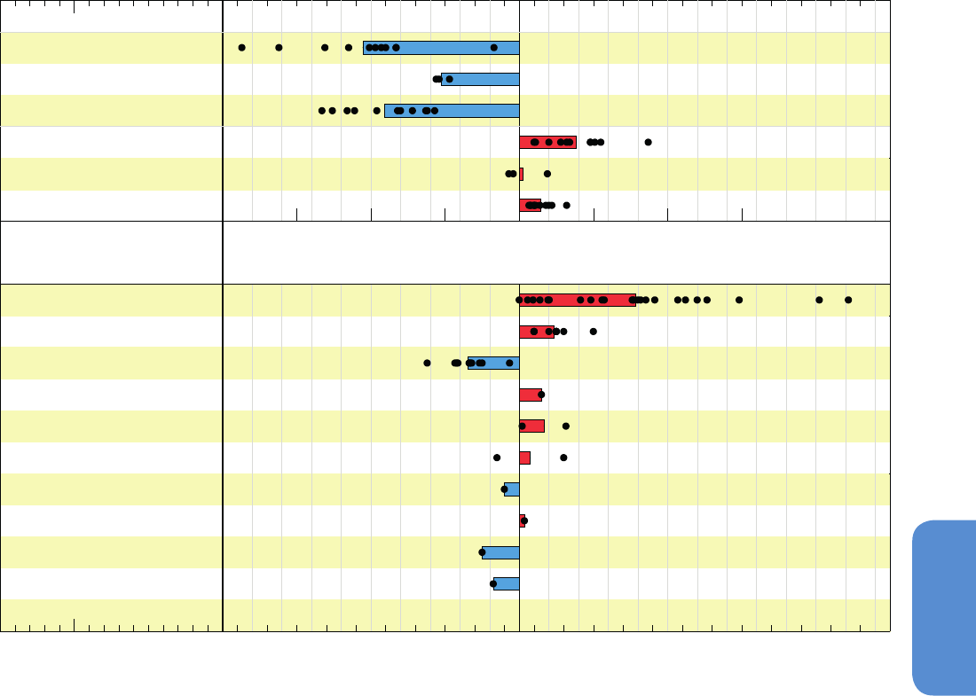
515
Carbon and Other Biogeochemical Cycles Chapter 6
6
Figure 6.20 | A synthesis of the magnitude of biogeochemical feedbacks on climate. Gregory et al. (2009) proposed a framework for expressing non-climate feedbacks in common
units (W m
–2
°C
–1
) with physical feedbacks, and Arneth et al. (2010) extended this beyond carbon cycle feedbacks to other terrestrial biogeochemical feedbacks. The figure shows
the results compiled by Arneth et al. (2010), with ocean carbon feedbacks from the C4MIP coupled climate–carbon models used for AR4 also added. Some further biogeochemical
feedbacks are also shown but this list is not exhaustive. Black dots represent single estimates, and coloured bars denote the simple mean of the dots with no weighting or assess-
ment being made to likelihood of any single estimate. There is low confidence in the magnitude of the feedbacks in the lower portion of the figure, especially for those with few, or
only one, dot. The role of nitrogen limitation on terrestrial carbon sinks is also shown—this is not a separate feedback, but rather a modulation to the climate–carbon and concentra-
tion–carbon feedbacks. These feedback metrics are also to be state or scenario dependent and so cannot always be compared like-for-like (see Section 6.4.2.2). Results have been
compiled from (a) Arneth et al. (2010), (b) Friedlingstein et al. (2006), (c) Hadley Centre Global Environmental Model 2-Earth System (HadGEM2-ES, Collins et al., 2011) simulations,
(d) Burke et al. (2013), (e) von Deimling et al. (2012), (f) Stocker et al. (2013), (g) Stevenson et al. (2006). Note the different x-axis scale for the lower portion of the figure.
-0.4 -0.2 0 0.2 0.4
W m
-2
K
-1
-0.4 -0.2 0 0.2 0.4
W m
-2
K
-1
-1.5 -1 -0.5 0 0.5 1 1.5
W m
-2
K
-1
Land C response to CO
2
(a,b)
including N-cycle
(a)
Ocean C response to CO
2
(b)
Land C response to climate
(a,b)
including N-cycle
(a)
Ocean C response to climate
(b)
Permafrost CO
2
(a,d,e)
Wetlands CH
4
(a,c,f)
Climate CH
4
lifetime
(c,g)
Climate on N
2
O
(f)
BVOC on ozone
(a)
fire
(a)
climate-aerosol
(c)
climate-ozone
(c)
climate-dust
(c)
climate-DMS
(c)
)(
)(
The climate–carbon response (γ) determines changes in carbon storage
due to changes in climate, and the concentration–carbon response (β)
determines changes in storage due to elevated CO
2
. Climate–carbon
cycle feedback responses have been analyzed for eight CMIP5 ESMs
that performed idealised simulations involving atmospheric CO
2
increasing at a prescribed rate of 1% yr
–1
(Arora et al., 2013; Box 6.4).
There is high confidence that increased atmospheric CO
2
will lead to
increased land and ocean carbon uptake but by an uncertain amount.
Models agree on the sign of land and ocean response to rising CO
2
but
show only medium and low agreement for the magnitude of ocean and
land carbon uptake respectively (Figure 6.21). Future climate change
will decrease land and ocean carbon uptake compared to the case
with constant climate (medium confidence). Models agree on the sign,
globally, of land and ocean response to climate change but show low
agreement on the magnitude of this response, especially for the land.
Land and ocean carbon uptake may differ in sign between different
regions and between models (Section 6.4.2.3). Inclusion of nitrogen
cycle processes in two of the land carbon cycle model components out
of these eight reduces the magnitude of the sensitivity to both CO
2
and
climate (Section 6.4.6.3) and increases the spread across the CMIP5
ensemble. The CMIP5 spread in ocean sensitivity to CO
2
and climate
appears reduced compared with C4MIP.
The role of the idealised experiment presented here is to study model
processes and understand what causes the differences between models.
Arora et al. (2013) assessed the global carbon budget from these ide-
alised simulations and found that the CO
2
contribution to changes in
land and ocean carbon storage sensitivity is typically four to five times
larger than the sensitivity to climate across the CMIP5 ESMs. The land
carbon-climate response (γ) is larger than the ocean carbon–climate

516
Chapter 6 Carbon and Other Biogeochemical Cycles
6
Box 6.4 | Climate–Carbon Cycle Models and Experimental Design
What are coupled climate–carbon cycle models and why do we need them?
Atmosphere–Ocean General Circulation Models (AOGCMs; see Glossary) have long been used for making climate projections, and
have formed the core of previous IPCC climate projection chapters (e.g., Meehl et al. (2007); see also Chapters 1, 9 and 12). For the 5th
Coupled Model Intercomparison Project (CMIP5), many models now have an interactive carbon cycle. What exactly does this mean,
how do they work and how does their use differ from previous climate models? AOGCMs typically represent the physical behaviour
of the atmosphere and oceans but atmospheric composition, such as the amount of CO
2
in the atmosphere, is prescribed as an input
to the model. This approach neglects the fact that changes in climate might affect the natural biogeochemical cycles, which control
atmospheric composition, and so there is a need to represent these processes in climate projections.
At the core of coupled climate–carbon cycle models is the physical climate model, but additional components of land and ocean
biogeochemistry respond to the changes in the climate conditions to influence in return the atmospheric CO
2
concentration. Input to
themodels comes in the form of anthropogenic CO
2
emissions, which can increase the CO
2
and then the natural carbon cycle exchanges
CO
2
between the atmosphere and land and ocean components. These ‘climate–carbon cycle models’ (‘Earth System Models’, ESMs; see
Glossary) provide a predictive link between fossil fuel CO
2
emissions and future CO
2
concentrations and climate and are an important
part of the CMIP5 experimental design (Hibbard et al., 2007; Taylor et al., 2012).
Apart from Earth System GCMs, so-called Earth System Models of Intermediate Complexity (EMICs) are often used to perform similar
experiments (Claussen et al., 2002; Plattner et al., 2008). EMICs have reduced resolution or complexity but run much more quickly and
can be used for longer experiments or large ensembles.
How are these models used?
The capability of ESMs to simulate carbon cycle processes and feedbacks, and in some models other biogeochemical cycles, allows for
a greater range of quantities to be simulated such as changes in natural carbon stores, fluxes or ecosystem functioning. There may also
be applications where it is desirable for a user to predefine the pathway of atmospheric CO
2
and prescribe it as a forcing to the ESMs.
Thus, numerical simulations with ESM models can be either ‘concentration driven’ or ‘emissions driven’.
Concentration-driven simulations follow the ‘traditional’ approach of prescribing the time-evolution of atmospheric CO
2
as an input to
the model. This is shown schematically in Box 6.4 Figure 1 (left-hand side). Atmospheric CO
2
concentration is prescribed as input to the
model from a given scenario and follows a predefined pathway regardless of changes in the climate or natural carbon cycle processes.
The processes between the horizontal dashed lines in the figure represent the model components which are calculated during the
concentration-driven simulation. Externally prescribed changes in atmospheric CO
2
concentration, which drive climate change, affect
land and ocean carbon storage. By construction, changes in land and ocean storage, however, do not feed back on the atmospheric CO
2
concentration or on climate. The changes in natural carbon fluxes and stores are output by the model.
So-called ‘compatible fossil fuel emissions’, E, can be diagnosed afterwards from mass conservation by calculating the residual between
the prescribed CO
2
pathway and the natural fluxes:
(6.1)
Land use change emissions cannot be diagnosed separately from a single simulation (see Section 6.4.3.2).
Emissions-driven simulations allow the full range of interactions in the models to operate and determine the evolution of atmospheric
CO
2
and climate as an internal part of the simulation itself (Box 6.4, Figure 1, right-hand side). In this case emissions of CO
2
are the
externally prescribed input to the model and the subsequent changes in atmospheric CO
2
concentration are simulated by it.
In emissions-driven experiments, the global atmospheric CO
2
growth rate is calculated within the model as a result of the net balance
between the anthropogenic emissions, E, and natural fluxes:
(6.2)
The effect of climate change on the natural carbon cycle will manifest itself either through changes in atmospheric CO
2
in the emis-
sions-driven experiments or in the compatible emissions in the concentration-driven experiments.
E =
dCO
2
dt
prescribed
+ (land_carbon_uptake + ocean_carbon_uptake)
dCO
2
dt
simulated
= E – (land_carbon_uptake + ocean_carbon_uptake)
(continued on next page)
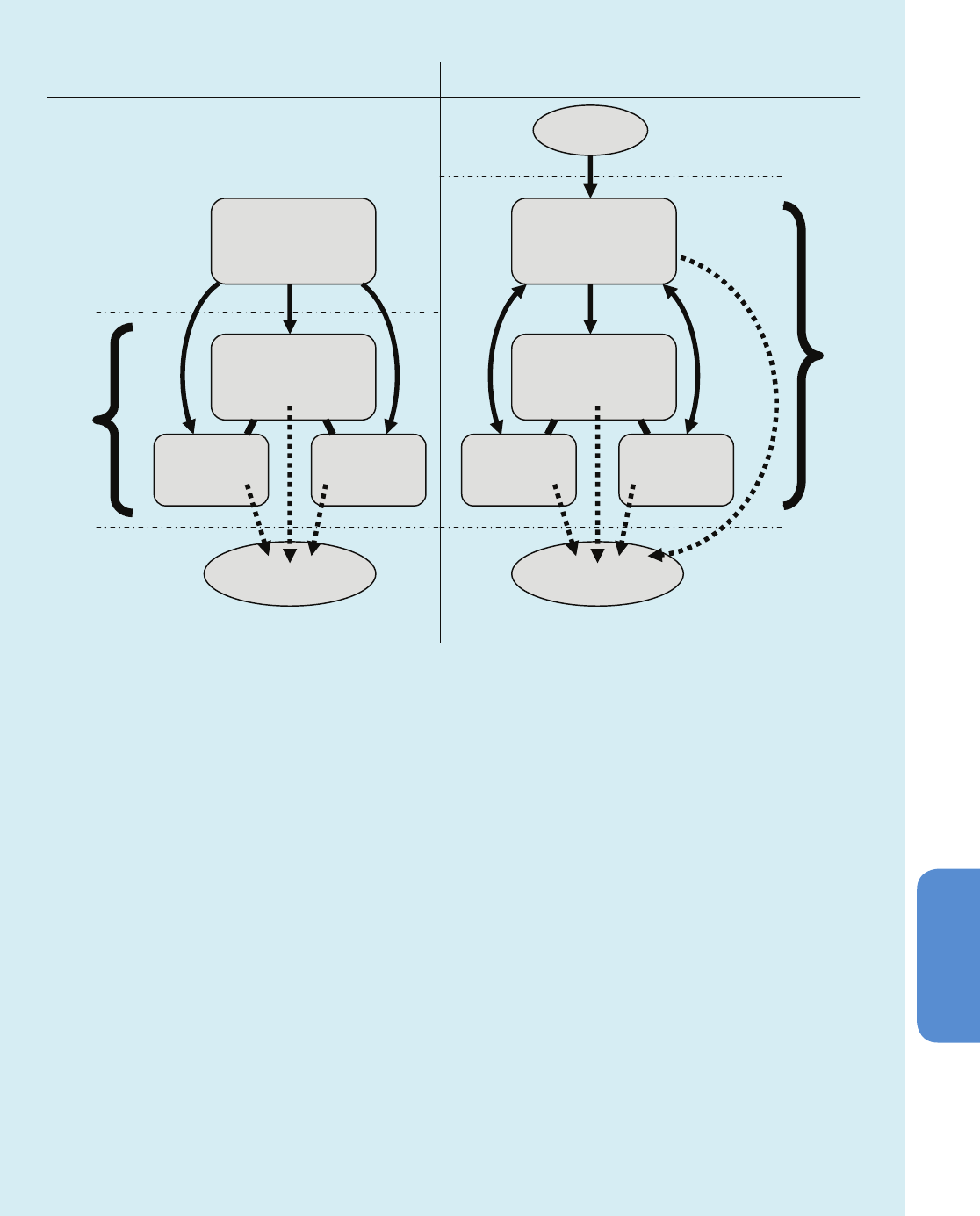
517
Carbon and Other Biogeochemical Cycles Chapter 6
6
Concentration-driven simulation experiments have the advantage that they can also be performed by GCMs without an interactive-
carbon cycle and have been used extensively in previous assessments (e.g., Prentice et al., 2001). For this reason, most of the Repre-
sentative Concentration Pathway (RCP) simulations (see Chapter 1) presented later in this chapter with carbon cycle models and in
Chapter 12 with models that do not all have an interactive carbon cycle are performed this way. Emissions-driven simulations have the
advantage of representing the full range of interactions in the coupled climate–carbon cycle models. The RCP8.5 pathway was repeated
by many ESM models as an emissions-driven simulation (Chapter 12).
Feedback Analysis
The ESMs are made up of many ‘components’, corresponding to different processes or aspects of the system. To understand their behav-
iour, techniques have been applied to assess different aspects of the models’ sensitivities (Friedlingstein et al., 2003, 2006; Arora et al.,
2013). The two dominant emerging interactions are the sensitivity of the carbon cycle to changes in CO
2
and its sensitivity to changes
in climate. These can be measured using two metrics: ‘beta’ (β) measures the strength of changes in carbon fluxes by land or ocean in
response to changes in atmospheric CO
2
;
‘gamma’ (γ) measures the strength of changes in carbon fluxes by land or ocean in response
to changes in climate. These metrics can be calculated as cumulative changes in carbon storage (as in Friedlingstein et al., 2006) or
instantaneous rates of change (Arora et al., 2013).
It is not possible to calculate these sensitivities in a single simulation, so it is necessary to perform ‘decoupled’ simulations in which some
processes in the models are artificially disabled in order to be able to evaluate the changes in other processes. See Table 1 in Box 6.4.
Box 6.4 (continued)
Output
nevirD snoissimEnevirD noitartnecnoC
Atmospheric
CO
2
Atmospheric
CO
2
Land
Carbon
Cycle
Climate System
Climate System
Ocean
Carbon
Cycle
Land
Carbon
Cycle
Ocean
Carbon
Cycle
CO
2
emissions
Internal model processes
Internal model processes
Output
Box 6.4, Figure 1 | Schematic representation of carbon cycle numerical experimental design. Concentration-driven (left) and emissions-driven (right) simulation
experiments make use of the same Earth System Models (ESMs), but configured differently. Concentration-driven simulations prescribe atmospheric CO
2
as a pre-
defined input to the climate and carbon cycle model components, but their output does not affect the CO
2
. Compatible emissions can be calculated from the output
of the concentration-driven simulations. Emissions-driven simulations prescribe CO
2
emissions as the input and atmospheric CO
2
is an internally calculated element
of the ESM.
(continued on next page)

518
Chapter 6 Carbon and Other Biogeochemical Cycles
6
A large positive value of β denotes that a model responds to increasing CO
2
by simulating large increases in natural carbon sinks.
Negative values of γ denote that a model response to climate warming is to reduce CO
2
uptake from the atmosphere, while a positive
value means warming acts to increase CO
2
uptake. β and γ values are not specified in a model, but are properties that emerge from
the suite of complex processes represented in the model. The values of the β and γ metrics diagnosed from simulations can vary from
place to place within the same model (see Section 6.4.2.3), although it is the average over the whole globe that determines the global
extent of the climate–carbon cycle feedback.
Such an idealised analysis framework should be seen as a technique for assessing relative sensitivities of models and understand-
ing their differences, rather than as absolute measures of invariant system properties. By design, these experiments exclude land use
change.
The complex ESMs have new components and new processes beyond conventional AO GCMs and thus require additional evaluation
to assess their ability to make climate projections. Evaluation of the carbon cycle model components of ESMs is presented in Section
6.3.2.5.6 for ocean carbon models and Section 6.3.2.6.6 for land carbon models. Evaluation of the fully coupled ESMs is presented in
Chapter 9.
Box 6.4, Table 1 | Configurations of simulations designed for feedback analysis by allowing some carbon–climate interactions to operate but holding others
constant. The curves denote whether increasing or constant CO
2
values are input to the radiation and carbon cycle model components. In a fully coupled simulation,
the carbon cycle components of the models experience both changes in atmospheric CO
2
(see Box 6.3 on fertilisation) and changes in climate. In ‘biogeochemically’
coupled experiments, the atmospheric radiation experiences constant CO
2
(i.e., the radiative forcing of increased CO
2
is not activated in the simulation) whereas the
carbon cycle model components experience increasing CO
2
. This experiment quantifies the strength of the effect of rising CO
2
concentration alone on the carbon cycle
(β). In a radiatively coupled experiment, the climate model’s radiation scheme experiences an increase in the radiative forcing of CO
2
(and hence produces a change
in climate) but CO
2
concentration is kept fixed to pre-industrial value as input to the carbon cycle model components. This simulation quantifies the effect of climate
change alone on the carbon cycle (γ).
Box 6.4 (continued)
CO
2
input to
radiation scheme
CO
2
input to carbon-
cycle scheme
Reason
Fully coupled Simulates the fully coupled system
‘Biogeochemically’
coupled
‘esmFixClim’
Isolates the carbon-cycle response to CO
2
(β) for land and oceans
Radiatively coupled
‘esmFdbk’
Isolates carbon-cycle response to climate
change (γ) for land and for oceans

519
Carbon and Other Biogeochemical Cycles Chapter 6
6
Time Period Duration Land Ocean Section
Climate CO
2
Land Use Climate CO
2
Seasonal cycle Weeks to months 3–8
a
2 1 6.3.2.5.1
+ +
Interannual
variability
Months to years 2–4
b
1 0.2 6.3.2.5.4
– + +
Historical
(1750–Present)
Decades to
centuries
150
c
–180 2 155 6.3.2.5.3, Table 6.1
– + ? +
21st Century
Decades to
centuries
100–400
d
–100 to +100
e
100–600
d
6.4.3
– + – +
Little Ice
Age (LIA)
f
Century +5 +2 to +30 6.2.3
– +
Holocene 10 kyr +300 –50 to –150 +270 to –220
g
6.2.2
+ +
Last Glacial
Maximum/
glacial cycles
>10 kyr +300 to +1000
h
–500 to –1200
h
6.2.1
+ + – +
Pulse
i
, 100 PgC 1 kyr +0 to +35 n/a +48 to +75 6.2.2
+ – +
Table 6.10 | Comparison of the sign and magnitude of changes in carbon storage (PgC) by land and ocean over different time scales. These changes are shown as approximate
numbers to allow a comparison across time scales. For more details see the indicated chapter section. An indication, where known, of what causes these changes (climate, CO
2
, land
use change) is also given with an indication of the sign: ‘+’ means that an increase in CO
2
or global-mean temperature is associated with an increase in carbon storage (positive β
or γ; see Section 6.4.2), and a ‘–’ means an increase in CO
2
or global-mean temperature is associated with a decrease in carbon storage (negative β or γ). The processes that oper-
ate to drive these changes can vary markedly, for example, from seasonal phenology of vegetation to long-term changes in ice sheet cover or ocean circulation impacting carbon
reservoirs. Some of these processes are ‘reversible’ in the context that they can increase and decrease cyclically, whereas some are ‘irreversible’ in the context that changes in one
sense might be much longer than in the opposite direction.
Notes:
a
Dominated by northern mid to high latitudes.
b
Dominated by the tropics.
c
‘Residual land sink’, Table 6.1.
d
Varies widely according to scenario. Climate effect estimated separately for RCP4.5 as –157 PgC (combined land and ocean), but not for other scenarios.
e
Future scenarios may increase or decrease area of anthropogenic land use.
f
Little Ice Age, 1500–1750.
g
Shown here are two competing drivers of Holocene ocean carbon changes: carbonate accumulation on shelves (coral growth) and carbonate compensation to pre-Holocene changes. These are
discussed in Section 6.2.2.
h
Defined as positive if increasing from LGM to present, negative if decreasing.
i
Idealised simulations with models to assess the response of the global carbon cycle to a sudden release of 100 PgC.
response in all models. Although land and ocean
contribute equally to
the total carbon–concentration response (β), the model spread in the
land response is greater than for the ocean.
6.4.2.2 Scenario Dependence of Feedbacks
The values of carbon-cycle feedback metrics can vary markedly for
different scenarios and as such cannot be used to compare model
simulations over different time periods, nor to inter-compare model
simulations with different scenarios (Arora et al., 2013). Gregory et al.
(2009) demonstrated how sensitive the feedback metrics are to the
rate of change of CO
2
for two models: faster rates of CO
2
increase lead
to reduced β values as the carbon uptake (especially in the ocean) lags
further behind the forcing. γ is much less sensitive to the scenario, as
both global temperature and carbon uptake lag the forcing.
6.4.2.3 Regional Feedback Analysis
The linear feedback analysis with the β and γ metrics of Friedlingstein
et al. (2006) has been applied at the regional scale to future carbon
uptake by Roy et al. (2011) and Yoshikawa et al. (2008). Figure 6.22
shows this analysis extended to land and ocean points for the CMIP5
models under the 1% yr
–1
CO
2
simulations.
6.4.2.3.1 Regional ocean response
Increased CO
2
is projected by the CMIP5 models to increase oceanic
CO
2
sinks almost everywhere (positive β) (high confidence) with the
exception of some very limited areas (Figure 6.22). The spatial distribu-
tion of the CO
2
ocean response, β
o
, is consistent between the models
and with the Roy et al. (2011) analysis. On average, the regions with
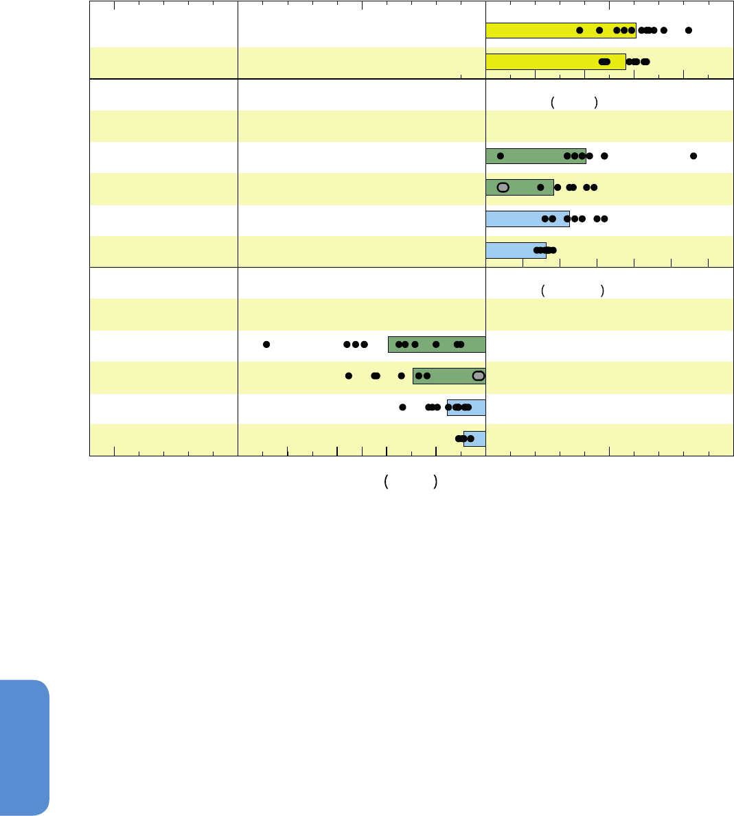
520
Chapter 6 Carbon and Other Biogeochemical Cycles
6
0.002 0.004 0.006 0.008
K ppm
-1
0.5 1.0 1.5 2.0 2.5 3.0
PgC ppm
-1
-200 -160 -120 -80 -40 0
PgC K
-1
Climate response
to CO
2
C4MIP
CMIP5
Land C
response to CO
2
Ocean C
response to CO
2
C4MIP
CMIP5
C4MIP
CMIP5
Land C
response to climate
Ocean C
response to climate
C4MIP
CMIP5
C4MIP
CMIP5
Figure 6.21 | Comparison of carbon cycle feedback metrics between the C4MIP ensemble of seven GCMs and four EMICs under the Special Report on Emission Scenario-A2
(SRES-A2) (Friedlingstein et al., 2006) and the eight CMIP5 models (Arora et al., 2013) under the 140-year 1% CO
2
increase per year scenario. Black dots represent a single model
simulation and coloured bars the mean of the multi-model results; grey dots are used for models with a coupled terrestrial nitrogen cycle. The comparison with C4MIP is for context,
but these metrics are known to be variable across different scenarios and rates of change (see Section 6.4.2.2). Some of the CMIP5 models are derived from models that contributed
to C4MIP and some are new to this analysis. Table 6.11 lists the main attributes of each CMIP5 model used in this analysis. The SRES A2 scenario is closer in rate of change to a
0.5% yr
–1
scenario and as such it should be expected that the CMIP5 γ terms are comparable, but the β terms are likely to be around 20% smaller for CMIP5 than for C4MIP due to
lags in the ability of the land and ocean to respond to higher rates of CO
2
increase (Gregory et al., 2009). This dependence on scenario (Section 6.4.2.2) reduces confidence in any
quantitative statements of how CMIP5 carbon cycle feedbacks differ from C4MIP. CMIP5 models used: Max Planck Institute–Earth System Model–Low Resolution (MPI–ESM–LR),
Beijing Climate Center–Climate System Model 1 (BCC–CSM1), Hadley Centre Global Environmental Model 2–Earth System (HadGEM2–ES), Institute Pierre Simon Laplace–Coupled
Model 5A–Low Resolution (IPSL–CM5A–LR), Canadian Earth System Model 2 (CanESM2), Norwegian Earth System Model– intermediate resolution with carbon cycle (NorESM–
ME), Community Earth System Model 1–Biogeochemical (CESM1–BGC), Model for Interdisciplinary Research On Climate–Earth System Model (MIROC–ESM).
the strongest increase of oceanic CO
2
sinks in response to higher
atmospheric CO
2
are the North Atlantic and the Southern Oceans. The
magnitude and distribution of β
o
in the ocean closely resemble the
distribution of historical anthropogenic CO
2
flux from inversion studies
and forward modelling studies (Gruber et al., 2009), with the dominant
anthropogenic CO
2
uptake in the Southern Ocean (Section 6.3.2.5).
Climate warming is projected by the CMIP5 models to reduce oceanic
carbon uptake in most oceanic regions (negative γ) (medium confi-
dence) consistent with the Roy et al. (2011) analysis (Figure 6.22).
This sensitivity of ocean CO
2
sinks to climate, γ
o
, is mostly negative
(i.e., a reduced regional ocean CO
2
sink in response to climate change)
but with regions of positive values in the Arctic, the Antarctic and in
the equatorial Pacific (i.e., climate change increases ocean CO
2
sink in
these regions). The North Atlantic Ocean and the mid-latitude Southern
Ocean have the largest negative γ
o
values. Reduced CO
2
uptake in
response to climate change in the sub-polar Southern Ocean and the
tropical regions has been attributed to warming induced decreased
CO
2
solubility, reduced CO
2
uptake in the mid latitudes to decreased
CO
2
solubility and decreased water mass formation which reduces the
absorption of anthropogenic CO
2
in intermediate and deep waters (Roy
et al., 2011). Increased uptake in the Arctic Ocean and the polar South-
ern Ocean is partly associated with a reduction in the fractional sea ice
coverage (Roy et al., 2011).
6.4.2.3.2 Regional land response
Increased CO
2
is projected by the CMIP5 models to increase land CO
2
sinks everywhere (positive β) (medium confidence). This response, β
L
,
has the largest values over tropical land, in humid rather than arid

521
Carbon and Other Biogeochemical Cycles Chapter 6
6
Model Modelling
Centre
Atmos
Resolution
Ocean
Resolution
Land-Carbon Ocean Carbon Reference
Model
Name
Dynamic
Vegetation
Cover?
No. of
PFTs
Incl. LUC?
Nitrogen-
Cycle
Fire
Model
Name
No. of
Plankton Types
Micronutrients?
BCC-CSM1.1 BCC ≈2.8
o
, L26 0.3–1
o
, L40 BCC_AVIM1.0 N 15 N N OCMIP2 n/a n/a Wu et al. (2013)
CanESM2 CCCma T63, L35 1.41° ×
0.94°, L40
CTEM N 9 Y N N CMOC 1 N Arora et al. (2011)
CESM1-BGC NSF-DOE-NCAR FV 0.9 × 1.25 1° CLM4 N 15 Y Y Y BEC 4 Y Long et al. (2013)
GFDL-ESM2G NOAA GFDL 2 × 2.5
o
, L24 1
o
, tri-polar,
1/3
o
at equa-
tor, L63.
LM3 Y 5 Y N Y TOPAZ2 6 y Dunne et al. (2012);
Dunne et al. (2013)
GFDL-ESM2M NOAA GFDL 2 × 2.5
o
, L24 1
o
, tri-polar,
1/3
o
at equa-
tor, L50.
LM3 Y 5 Y N Y TOPAZ2 6 y Dunne et al. (2012);
Dunne et al. (2013)
HadGEM2-ES MOHC N96 (~
1.6°), L38
1
o
, 1/3
o
at
equator, L40
JULES Y 5 Y N N Diat-
HadOCC
3 Y Collins et al. (2011);
Jones et al. (2011)
INMCM4 INM
IPSL-CM5A-LR IPSL 3.75 × 1.9 , L39 Zonal 2°,
Meridional
2°–0.5° L31
ORCHIDEE N 13 Y N Y PISCES 2 Y Dufresne et al. (2013)
MIROC-ESM MIROC T42, L80 Zonal: 1.4
o
,
Meridional:
0.5–1.7
o
,
Vertical:
L43+BBL1
SEIB-DGVM Y 13 Y N N NPZD
(Oschlies,
2001)
2 (Phyoto-
plankton and
Zoolo-plankton)
N Watanabe et al. (2011)
MPI-ESM-LR MPI-M T63 (~
1.9°), L47
ca.1.5°, L47 JSBACH Y 12 (8
natural)
Y N Y HAMOCC 2 Y Raddatz et al.
(2007), Brovkin et
al. (2009), Maier-
Reimer et al. (2005)
NorESM-ME NCC 1.9 × 2.5
o
, L26 1
o
, L53 CLM4 N 16 Y Y Y HAMOCC 2 N Iversen et al. (2013)
Table 6.11 | CMIP5 model descriptions in terms of carbon cycle attributes and processes.
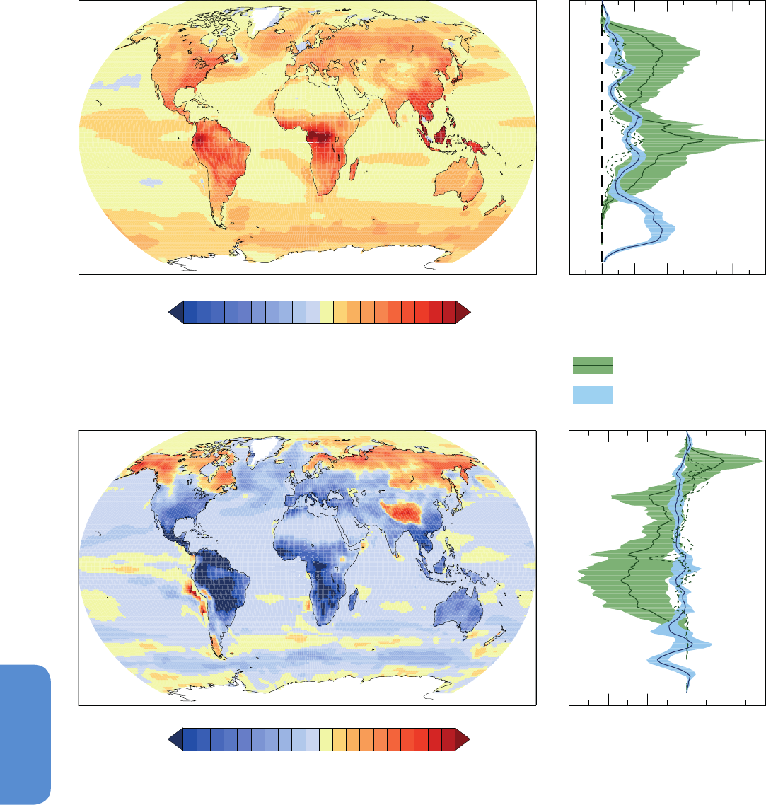
522
Chapter 6 Carbon and Other Biogeochemical Cycles
6
Figure 6.22 | The spatial distributions of multi-model-mean land and ocean β and γ for seven CMIP5 models using the concentration-driven idealised 1% yr
–1
CO
2
simulations.
For land and ocean, β and γ are defined from changes in terrestrial carbon storage and changes in air–sea integrated fluxes respectively, from 1 × CO
2
to 4 × CO
2
, relative to global
(not local) CO
2
and temperature change. In the zonal mean plots, the solid lines show the multi-model mean and shaded areas denote ±1 standard deviation. Models used: Beijing
Climate Center–Climate System Model 1 (BCC–CSM1), Canadian Earth System Model 2 (CanESM2), Community Earth System Model 1–Biogeochemical (CESM1–BGC), Hadley
Centre Global Environmental Model 2–Earth System (HadGEM2–ES), Institute Pierre Simon Laplace– Coupled Model 5A–Low Resolution (IPSL–CM5A-LR), Max Planck Institute–
Earth System Model–Low Resolution (MPI–ESM–LR), Norwegian Earth System Model 1 (Emissions capable) (NorESM1–ME). The dashed lines show the models that include a land
carbon component with an explicit representation of nitrogen cycle processes (CESM1-BGC, NorESM1-ME).
a. Regional carbon-concentration feedback
0 0.10 0.20
Land
Ocean
(10
6
kgC m
-1
ppm
-1
)
(kgC m
-2
ppm
-1
)
41220-4-12-20
b. Regional carbon-climate feedback
-10
01
0
(10
6
kgC m
-1
K
-1
)
(kgC m
-2
K
-1
)
0 0.5 1-0.5-1
x 10
-3

523
Carbon and Other Biogeochemical Cycles Chapter 6
6
regions, associated with enhanced carbon uptake in forested areas of
already high biomass. In the zonal totals, there is a secondary peak of
high β
L
values over NH temperate and boreal ecosystems, partly due to
a greater land area there but also coincident with large areas of forest.
Models agree on the sign of response but have low agreement on the
magnitude.
The climate effect alone is projected by the CMIP5 models to reduce
land CO
2
sinks in tropics and mid latitudes (negative γ) (medium
confidence). CMIP5 models show medium agreement that warming
may increase land carbon uptake in high latitudes but none of these
models include representation of permafrost carbon pools which are
projected to decrease in warmer conditions (Section 6.4.3.3); there-
fore confidence is low regarding the sign and magnitude of future
high-latitude land carbon response to climate change. Matthews et
al. (2005) showed that vegetation productivity is the major cause of
C4MIP model spread, but this manifests itself as changes in soil organ-
ic matter (Jones and Falloon, 2009).
6.4.3 Implications of the Future Projections for the
Carbon Cycle and Compatible Emissions
6.4.3.1 The RCP Future Carbon Dioxide Concentration
and Emissions Scenarios
The CMIP5 simulations include four future scenarios referred to as
Representative Concentration Pathways (RCPs; see Glossary) (Moss
et al., 2010): RCP2.6, RCP4.5, RCP6.0, RCP8.5 (see Chapter 1). These
future scenarios include CO
2
concentration and emissions, and have
been generated by four Integrated Assessment Models (IAMs) and are
labelled according to the approximate global radiative forcing level at
2100. These scenarios are described in more detail in Chapter 1 (Box
1.1) and Section 12.3 and also documented in Annex II.
van Vuuren et al. (2011) showed that the basic climate and carbon cycle
responses of IAMs is generally consistent with the spread of climate and
carbon cycle responses from ESMs. For the physical and biogeochemical
components of the RCP scenarios 4.5, 6.0 and 8.5, the underlying IAMs
are closely related. Only the Integrated Model to Assess the Global Envi-
ronment (IMAGE) IAM, which created RCP2.6, differs markedly by using
a more sophisticated carbon cycle sub-model for land and ocean. The
Model for the Assessment of Greenhouse-gas Induced Climate Change
6 (MAGICC6) simple climate model was subsequently used to generate
the CO
2
pathway for all four RCP scenarios using the CO
2
emissions
output by the four IAMs (Meinshausen et al., 2011).
6.4.3.2 Land Use Changes in Future Scenarios
ESMs and IAMs use a diversity of approaches for representing land
use changes, including different land use classifications, parameter
settings, and geographical scales. To implement land use change in a
consistent manner across ESMs, a ‘harmonized’ set of annual gridded
land use change during the period 1500–2100 was developed for input
to the CMIP5 ESMs (Hurtt et al., 2011).
Not all the CMIP5 ESMs used the full range of information available
from the land use change scenarios, such as wood harvest projections
or sub-grid scale shifting cultivation. Sensitivity studies indicated that
these processes, along with the start date of the simulation, all strongly
affect estimated carbon fluxes (Hurtt et al., 2011; Sentman et al., 2011).
Land use has been in the past and will be in the future a significant
driver of forest land cover change and terrestrial carbon storage. Land
use trajectories in the RCPs show very distinct trends and cover a wide
range of projections. These land use trajectories are very sensitive to
assumptions made by each individual IAM regarding the amount of
land needed for food production (Figure 6.23). The area of cropland
and pasture increases in RCP8.5 with the Model for Energy Supply
Strategy Alternatives and their General Environmental Impact (MES-
SAGE) IAM model, mostly driven by an increasing global population,
but cropland area also increases in the RCP2.6 with the IMAGE IAM
model, as a result of bio-energy production and increased food demand
as well. RCP6 with the AIM model shows an expansion of cropland but
a decline in pasture land. RCP4.5 with the Global Change Assessment
Model (GCAM) IAM is the only scenario to show a decrease in global
cropland. Several studies (Wise et al., 2009; Thomson et al., 2010;
Tilman et al., 2011) highlight the large sensitivity of future land use
requirements to assumptions such as increases in crop yield, changes
in diet, or how agricultural technology and intensification is applied.
Within the IAMs, land use change is translated into land use CO
2
emis-
sions as shown in Figure 6.23(b). Cumulative emissions for the 21st
century (Figure 6.23c) vary markedly across RCPs, with increasing crop-
land and pastureland areas in RCP2.6 and RCP8.5 giving rise to the
highest emissions from land use change, RCP4.5 to intermediate emis-
sions and RCP6.0 to close to zero net emissions. All scenarios suggest
that 21st century land use emissions will be less than half of those
from 1850 to the present day as rate of change of land conversion
stabilises in future.
The adoption of widely differing approaches among ESMs for the treat-
ment and diagnosis of land use and land cover change (LULCC) pro-
cesses in terrestrial carbon cycle models leads to substantial between-
model variation in the simulated impact on land carbon stocks. It is
not yet possible to fully quantify LULCC fluxes from the CMIP5 model
simulations. The harmonization process applied to LULCC data sets for
CMIP5 has been an important step toward consistency among IAMs;
however, among ESMs, and between IAMs and ESMs, assignment of
meaningful uncertainty ranges to present-day and future LULCC fluxes
and states remains a critical knowledge gap with implications for com-
patible emissions to achieve CO
2
pathways (Section 6.4.3.3; Jones et
al., 2013).
6.4.3.3 Projections of Future Carbon Cycle Response by
Earth System Models Under the Representative
Concentration Pathway Scenarios
Simulated changes in land and ocean carbon uptake and storage under
the four RCP scenarios are presented here using results from CMIP5
ESMs concentration-driven simulations (see Box 6.4). The implications
of these changes on atmospheric CO
2
and climate as simulated by
CMIP5 emissions-driven simulations are presented in Chapter 12.
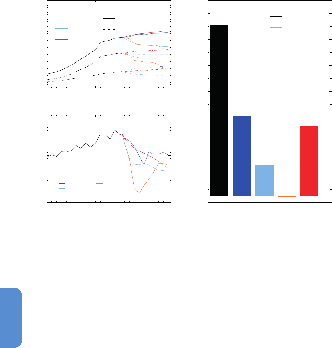
524
Chapter 6 Carbon and Other Biogeochemical Cycles
6
1850 1900 1950 2000 2050 2100
Year
0.0
0.1
0.2
0.3
0.4
0.5
Fraction of land
Global crop and pasture fraction
a
Historical
RCP2.6
RCP4.5
RCP6.0
RCP8.5
crop + pasture
pasture
crop
1850 1900 1950 2000 2050 2100
Year
-1.0
-0.5
0.0
0.5
1.0
1.5
PgC yr
-1
Land-use CO
2
emissions
b
Historical
RCP2.6
RCP4.5
RCP6.0
RCP8.5
Hist RCP2.6 RCP4.5 RCP6.0 RCP8.5
0
20
40
60
80
100
120
140
PgC
Cumulative land-use CO
2
emissions
c
Historical
RCP2.6
RCP4.5
RCP6.0
RCP8.5
( )
Figure 6.23 | Land use trends and CO
2
emissions according to the four different integrated assessment models (IAMs) used to define the RCP scenarios. Global changes in crop-
lands and pasture from the historical record and the RCP scenarios (top left), and associated annual land use emissions of CO
2
(bottom left). Bars (right panel) show cumulative
land use emissions for the historical period (defined here as 1850–2005) and the four RCP scenarios from 2006 to 2100.
The results of the concentration-driven CMIP5 ESMs simulations show
medium agreement on the magnitude of cumulative ocean carbon
uptake from 1850 to 2005 (Figure 6.24a): average 127 ± 28 PgC (1
standard deviation). The models show low agreement on the sign and
magnitude of changes in land carbon storage (Figure 6.24a): average
2 ± 74 PgC (1 standard deviation). These central estimates are very
close to observational estimates of 125 ± 25 PgC for the ocean and
–5 ± 40 PgC for the net cumulative land–atmosphere flux respectively
(see Table 6.12), but show a large spread across models. With very
high confidence, for all four RCP scenarios, all models project contin-
ued ocean uptake throughout the 21st century, with higher uptake
corresponding to higher concentration pathways. For RCP4.5, all the
models also project an increase in land carbon uptake, but for RCP2.6,
RCP6.0 and RCP8.5 a minority of models (4 out of 11 for RCP2.6, 1
out of 8 for RCP6.0 and 4 out of 15 for RCP8.5; Jones et al., 2013)
project a decrease in land carbon storage at 2100 relative to 2005.
Model spread in land carbon projections is much greater than model
spread in ocean carbon projections, at least in part due to different
treatment of land use change. Decade mean land and ocean fluxes are
documented in Annex II, Table AII.3.1a, b. Important processes missing
from many or all CMIP5 land carbon cycles include the role of nutrient
cycles, permafrost, fire and ecosystem acclimation to changing climate.
For this reason we assign low confidence to quantitative projections of
future land uptake.
The concentration-driven ESM simulations can be used to quantify
the compatible fossil fuel emissions required to follow the four RCP
CO
2
pathways (Jones et al., 2013; see Box 6.4, Figure 6.25, Table 6.12,
Annex II, Table AII.2.1a). There is significant spread between ESMs,
but general consistency between ESMs and compatible emissions
estimated by IAMs to define each RCP scenario. However, for RCP8.5
on average, the CMIP5 models project lower compatible emissions
than the MESSAGE IAM. The IMAGE IAM predicts that global negative
emissions are required to achieve the RCP2.6 decline in radiative forc-
ing from 3 W m
–2
to 2.6 W m
–2
by 2100. All models agree that strong
emissions reductions are required to achieve this after about 2020
(Jones et al., 2013). An average emission reduction of 50% (range 14
to 96%) is required by 2050 relative to 1990 levels. There is disagree-
ment between those ESMs that performed this simulation over the
necessity for global emissions in the RCP2.6 to become negative by
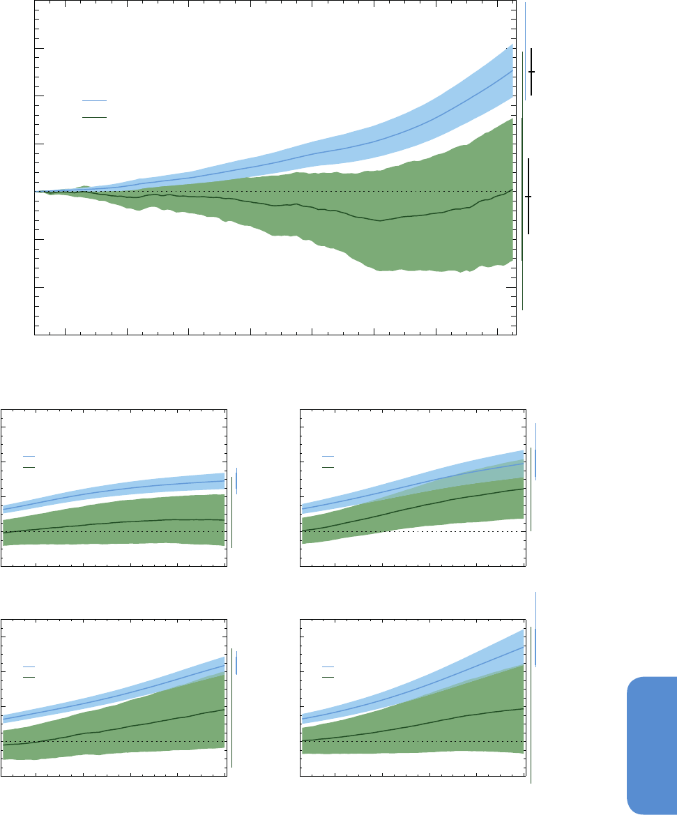
525
Carbon and Other Biogeochemical Cycles Chapter 6
6
1860 1880 1900 1920 1940 1960 1980 2000
Years
-150
-100
-50
0
50
100
150
200
Cumulative uptake (PgC)
Historical
a
ocean
land
2020 2040 2060 2080 2100
Years
-200
0
200
400
600
Cumulative uptake (PgC)
RCP2.6
b
ocean
land
2020 2040 2060 2080 2100
Years
-200
0
200
400
600
Cumulative uptake (PgC)
RCP4.5
c
ocean
land
2020 2040 2060 2080 2100
Years
-200
0
200
400
600
Cumulative uptake (PgC)
RCP6.0
d
ocean
land
2020 2040 2060 2080 2100
Years
-200
0
200
400
600
Cumulative uptake (PgC)
RCP8.5
e
ocean
land
Figure 6.24 | Cumulative land and ocean carbon uptake simulated for the historical period 1850–2005 (top) and for the four RCP scenarios up to 2100 (b–e). Mean (thick
line) and 1 standard deviation (shaded). Vertical bars on the right show the full model range as well as standard deviation. Black bars show observationally derived estimates for
2005. Models used: Canadian Earth System Model 2 (CanESM2), Geophysical Fluid Dynamics Laboratory–Earth System Model 2G (GFDL–ESM2G), Geophysical Fluid Dynamics
Laboratory–Earth System Model 2M (GFDL–ESM2M), Hadley Centre Global Environmental Model 2–Carbon Cycle (HadGEM2-CC), Hadley Centre Global Environmental Model
2–Earth System (HadGEM2-ES), Institute Pierre Simon Laplace–Coupled Model 5A–Low Resolution (IPSL–CM5A–LR), Institute Pierre Simon Laplace–Coupled Model 5A–Medium
Resolution (IPSL–CM5A–MR), Institute Pierre Simon Laplace–Coupled Model 5B–Low Resolution (IPSL–CM5B–LR), Model for Interdisciplinary Research On Climate–Earth System
Model (MIROC–ESM–CHEM), Model for Interdisciplinary Research On Climate–Earth System Model (MIROC–ESM), Max Planck Institute–Earth System Model–Low Resolution
(MPI–ESM–LR), Norwegian Earth System Model 1 (Emissions capable) (NorESM1–ME), Institute for Numerical Mathematics Coupled Model 4 (INMCM4), Community Earth System
Model 1–Biogeochemical (CESM1–BGC), Beijing Climate Center–Climate System Model 1.1 (BCC–CSM1.1). Not every model performed every scenario simulation.

526
Chapter 6 Carbon and Other Biogeochemical Cycles
6
Compatible Fossil Fuel
Emissions Diagnosed from
Concentration-Driven CMIP5 Simulations
Land Carbon Changes Ocean Carbon Changes
Historical /
RCP Scenario
CMIP5 ESM
Mean
CMIP5 ESM
Range
Historical /
RCP Scenario
CMIP5 ESM
Mean
CMIP5 ESM
Range
Historical /
RCP Scenario
CMIP5 ESM
Mean
CMIP5 ESM
Range
1850–2011 375
a
350 235–455 5 ± 40
b
10 –125 to 160 140 ± 25
b
140 110–220
RCP2.6 275 270 140–410
c
65 –50 to 195
c
150 105–185
RCP4.5 735 780 595–1005 230 55 to 450 250 185–400
RCP6.0 1165 1060 840–1250 200 –80 to 370 295 265–335
RCP8.5 1855 1685 1415–1910 180 –165 to 500 400 320–635
Table 6.12 | The range of compatible fossil fuel emissions (PgC) simulated by the CMIP5 models for the historical period and the four RCP scenarios, expressed as cumulative
fossil fuel emission. To be consistent with Table 6.1 budgets are calculated up to 2011 for historical and 2012–2100 for future scenarios, and values are rounded to the nearest
5 PgC.
Notes:
a
Historical estimates of fossil fuel are as prescribed to all CMIP5 ESMs in the emissions-driven simulations (Andres et al., 2011).
b
Estimate of historical net land and ocean carbon uptake from Table 6.1 but over the shorter 1850–2011 time period.
c
IAM breakdown of future carbon changes by land and ocean are not available.
the end of the 21st century to achieve this, with six ESMs simulat-
ing negative compatible emissions and four ESM models simulating
positive emissions from 2080 to 2100. The RCP2.6 scenario achieves
this negative emission rate through use of large-scale bio-energy with
carbon-capture and storage (BECCS). It is as likely as not that sustained
globally negative emissions will be required to achieve the reductions
in atmospheric CO
2
in the RCP2.6 scenario. This would be classed as a
carbon dioxide removal (CDR) form of geoengineering under the defi-
nition used in this IPCC report, and is discussed further in Section 6.5.2.
The ESMs themselves make no assumptions about how the compatible
emissions could or would be achieved, but merely compute the global
total emission that is required to follow the CO
2
concentration path-
way, accounting for the carbon cycle response to climate and CO
2
, and
for land use change CO
2
emissions.
The dominant cause of future changes in the airborne fraction of fossil
fuel emissions (see Section 6.3.2.4) is the emissions scenario and not
carbon cycle feedbacks (Jones et al., 2013; Figure 6.26). Models show
high agreement that 21st century cumulative airborne fraction will
increase under rapidly increasing CO
2
in RCP8.5 and decreases under
the peak-and-decline RCP2.6 scenarios. The airborne fraction declines
slightly under RCP4.5 and remains of similar magnitude in the RCP6.0
scenario. Between-model spread in changes in the land-fraction is
greater than between-scenario spread. Models show high agreement
that the ocean fraction will increase under RCP2.6 and remain of simi-
lar magnitude in the other RCP scenarios.
Several studies (Jones et al., 2006; Matthews, 2006; Plattner et al.,
2008; Miyama and Kawamiya, 2009) have shown that climate–carbon
cycle feedbacks affect the compatible fossil fuel CO
2
emissions that are
consistent with a given CO
2
concentration pathway. Using decoupled
RCP4.5 simulations (see Box 6.4) five CMIP5 ESMs agree that the cli-
mate impact on carbon uptake by both land and oceans will reduce the
compatible fossil fuel CO
2
emissions for that scenario by between 6%
and 29% between 2006 and 2100 respectively (Figure 6.27), equating
to an average of 157 ± 76 PgC (1 standard deviation) less carbon that
can be emitted from fossil fuel use if climate feedback (see Glossary) is
included. Compatible emissions would be reduced by a greater degree
under higher CO
2
scenarios that exhibit a greater degree of climate
change (Jones et al., 2006).
6.4.3.4 Permafrost Carbon
Current estimates of permafrost soil carbon stocks are ~1700 PgC
(Tarnocai et al., 2009), the single largest component of the terrestrial
carbon pool. Terrestrial carbon models project a land CO
2
sink with
warming at high northern latitudes; however none of the models
participating in C4MIP or CMIP5 included explicit representation of
permafrost soil carbon decomposition in response to future warming.
Including permafrost carbon processes into an ESM may change the
sign of the high northern latitude carbon cycle response to warm-
ing from a sink to a source (Koven et al., 2011). Overall, there is high
confidence that reductions in permafrost extent due to warming will
cause thawing of some currently frozen carbon. However, there is low
confidence on the magnitude of carbon losses through CO
2
and CH
4
emissions to the atmosphere. The magnitude of CO
2
and CH
4
emissions
to the atmosphere is assessed to range from 50 to 250 PgC between
2000 and 2100 for RCP8.5. The magnitude of the source of CO
2
to the
atmosphere from decomposition of permafrost carbon in response to
warming varies widely according to different techniques and scenarios.
Process models provide different estimates of the cumulative loss of
permafrost carbon: 7 to 17 PgC (Zhuang et al., 2006) (not considered
in the range given above because it corresponds only to contemporary
tundra soil carbon), 55 to 69 Pg (Koven et al., 2011), 126 to 254 PgC
(Schaefer et al., 2011) and 68 to 508 PgC (MacDougall et al., 2012)
(not considered in the range given above because this estimate is not
obtained from a concentration driven, but for emission driven RCP sce-
nario and it is the only study of that type so far). Combining observed
vertical soil carbon profiles with modeled thaw rates provides an esti-
mate that the total quantity of newly thawed soil carbon by 2100 will
be 246 PgC for RCP4.5 and 436 PgC for RCP8.5 (Harden et al., 2012),
although not all of this amount will be released to the atmosphere on
that time scale. Uncertainty estimates suggest the cumulative amount
of thawed permafrost carbon could range from 33 to 114 PgC (68%
range) under RCP8.5 warming (Schneider von Deimling et al., 2012),
or 50 to 270 PgC (5th to 95th percentile range) (Burke et al., 2013).
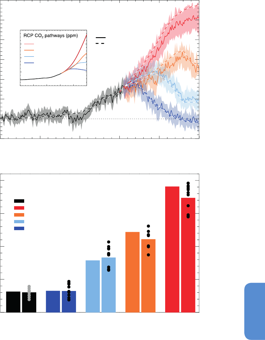
527
Carbon and Other Biogeochemical Cycles Chapter 6
6
1850 1900 1950 2000 2050 2100
Years
-5
0
5
10
15
20
25
30
(PgC yr
-1
)
Fossil-fuel emissions
RCP8.5
RCP6.0
RCP4.5
RCP2.6
CMIP5 mean
IAM scenario
1850 1900 1950 2000 2050 2100
200
400
600
800
1000
0
500
1000
1500
2000
(PgC)
Cumulative fossil-fuel emissions
Historical
ESMs
IMAGE
ESMs
GCAM
ESMs
AIM
ESMs
MESSAGE
ESMs
Historical emission inventories (1860-2005)
RCP8.5 (2006-2100)
RCP6.0 (2006-2100)
RCP4.5 (2006-2100)
RCP2.6 (2006-2100)
Figure 6.25 | Compatible fossil fuel emissions simulated by the CMIP5 ESMs for the four RCP scenarios. Top: time series of compatible emission rate (PgC yr
–1
). Dashed lines
represent the historical estimates and emissions calculated by the Integrated Assessment Models (IAMs) used to define the RCP scenarios, solid lines and plumes show results
from CMIP5 ESMs (model mean, with 1 standard deviation shaded). Bottom: cumulative emissions for the historical period (1860–2005) and 21st century (defined in CMIP5 as
2006–2100) for historical estimates and RCP scenarios. Dots denote individual ESM results, bars show the multi-model mean. In the CMIP5 model results, total carbon in the
land–atmosphere–ocean system can be tracked and changes in this total must equal fossil fuel emissions to the system (see Box 6.4). Models used: Canadian Earth System Model
2 (CanESM2), Geophysical Fluid Dynamics Laboratory–Earth System Model 2G (GFDL–ESM2G), Geophysical Fluid Dynamics Laboratory–Earth System Model 2M (GFDL–ESM2M),
Hadley Centre Global Environmental Model 2–Carbon Cycle(HadGEM2-CC), Hadley Centre Global Environmental Model 2–Earth System (HadGEM2-ES), Institute Pierre Simon
Laplace–Coupled Model 5A–Low Resolution (IPSL–CM5A–LR), Institute Pierre Simon Laplace–Coupled Model 5A–Medium Resolution (IPSL–CM5A–MR), Institute Pierre Simon
Laplace–Coupled Model 5B–Low Resolution (IPSL–CM5B–LR), Model for Interdisciplinary Research On Climate–Earth System Model (MIROC–ESM–CHEM), Model for Interdis-
ciplinary Research On Climate–Earth System Model (MIROC–ESM), Max Planck Institute–Earth System Model–Low Resolution (MPI–ESM–LR), Norwegian Earth System Model 1
(Emissions capable) (NorESM1–ME), Institute for Numerical Mathematics Coupled Model 4 (INMCM4), Community Earth System Model 1–Biogeochemical (CESM1–BGC), Beijing
Climate Center–Climate System Model 1.1 (BCC–CSM1.1). Not every model performed every scenario simulation.
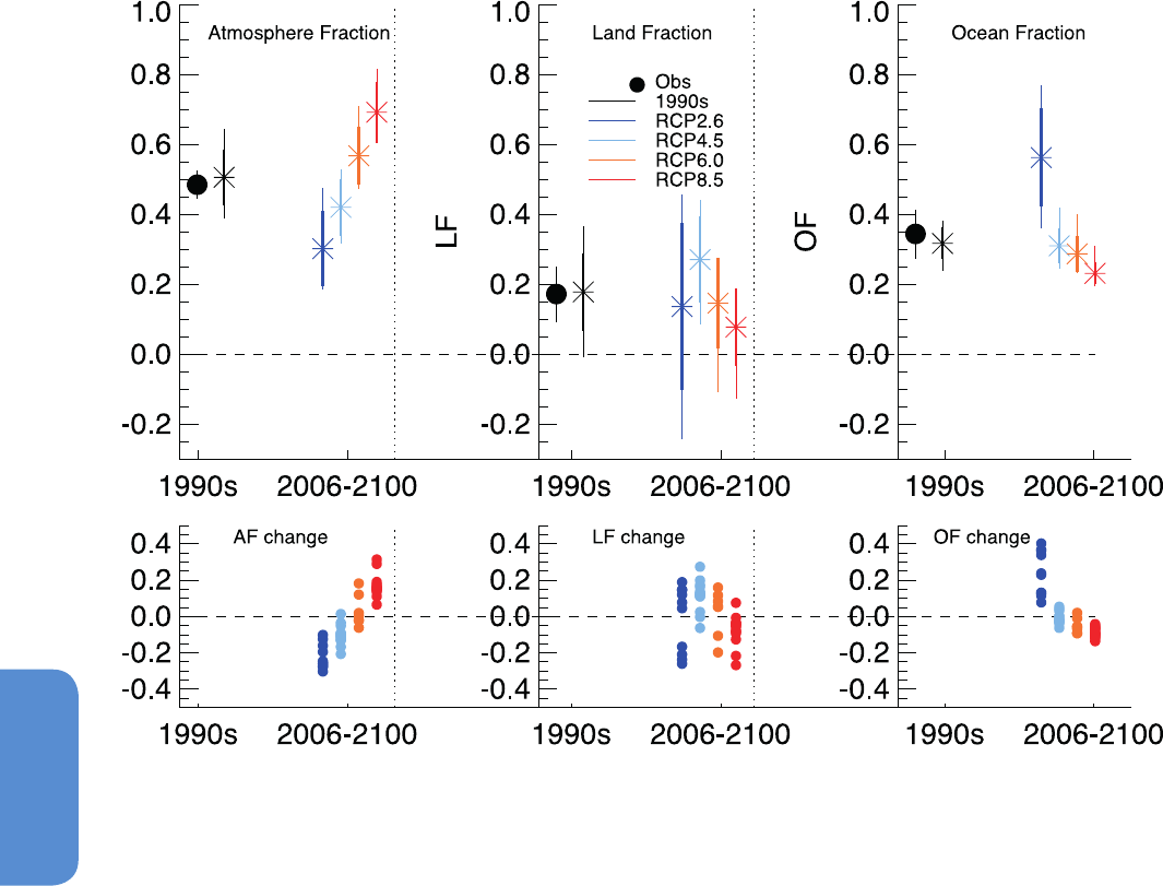
528
Chapter 6 Carbon and Other Biogeochemical Cycles
6
Figure 6.26 | Changes in atmospheric, land and ocean fraction of fossil fuel carbon emissions. The fractions are defined as the changes in storage in each component (atmosphere,
land, ocean) divided by the compatible fossil fuel emissions derived from each CMIP5 simulation for the four RCP scenarios. Solid circles show the observed estimate based on Table
6.1 for the 1990s. The coloured bars denote the cumulative uptake fractions for the 21st century under the different RCP scenarios for each model. Multi-model mean values are
shown as star symbols and the multi-model range (min-to-max) and standard deviation are shown by thin and thick vertical lines respectively. Owing to the difficulty of estimating
land use emissions from the ESMs this figure uses a fossil fuel definition of airborne fraction, rather than the preferred definition of fossil and land use emissions discussed in Sec-
tion 6.3.2.4. 21st century cumulative atmosphere, land and ocean fractions are shown here in preference to the more commonly shown instantaneous fractions because for RCP2.6
emissions reach and cross zero for some models and so an instantaneous definition of AF becomes singular at that point. Models used: Canadian Earth System Model 2 (CanESM2),
Geophysical Fluid Dynamics Laboratory–Earth System Model 2G (GFDL–ESM2G), Geophysical Fluid Dynamics Laboratory–Earth System Model 2M (GFDL–ESM2M), Hadley Centre
Global Environmental Model 2–Carbon Cycle (HadGEM2-CC), Hadley Centre Global Environmental Model 2–Earth System (HadGEM2-ES), Institute Pierre Simon Laplace–Coupled
Model 5A–Low Resolution (IPSL–CM5A–LR), Institute Pierre Simon Laplace–Coupled Model 5A–Medium Resolution (IPSL–CM5A–MR), Institute Pierre Simon Laplace–Coupled
Model 5B–Low Resolution (IPSL–CM5B–LR), Model for Interdisciplinary Research On Climate–Earth System Model (MIROC–ESM–CHEM), Model for Interdisciplinary Research On
Climate–Earth System Model (MIROC–ESM), Max Planck Institute–Earth System Model–Low Resolution (MPI–ESM–LR), Norwegian Earth System Model 1 (Emissions capable)
(NorESM1–ME), Institute for Numerical Mathematics Coupled Model 4 (INMCM4), Community Earth System Model 1–Biogeochemical (CESM1–BGC). Not every model performed
every scenario simulation.
Sources of uncertainty for the permafrost carbon feedback include the
physical thawing rates, the fraction of carbon that is released after
being thawed and the time scales of release, possible mitigating nutri-
ent feedbacks and the role of fine-scale processes such as spatial
variability in permafrost degradation. It is also uncertain how much
thawed carbon will decompose to CO
2
or to CH
4
(see Sections 6.4.7,
12.5.5.4 and 12.4.8.1).
6.4.4 Future Ocean Acidification
A fraction of CO
2
emitted to the atmosphere dissolves in the ocean,
reducing surface ocean pH and carbonate ion concentrations. The asso-
ciated chemistry response to a given change in CO
2
concentration is
known with very high confidence. Overall, given evidence from Chap-
ter 3 and model results from this chapter, it is virtually certain that the
increased storage of carbon by the ocean will increase acidification in
the future, continuing the observed trends of the past decades. Expect-
ed future changes are in line with what is measured at ocean time
series stations (see Chapter 3). Multi-model projections using ocean
process-based carbon cycle models discussed in AR4 demonstrate large
decreases in pH and carbonate ion concentration [CO
3
2–
] during the
21st century throughout the world oceans (Orr et al., 2005). The largest
decrease in surface [CO
3
2–
] occur in the warmer low and mid-latitudes,
which are naturally rich in this ion (Feely et al., 2009). However, it is
the low Ω
A
waters in the high latitudes and in the upwelling regions
that first become undersaturated with respect to aragonite (i.e., Ω
A
<1,
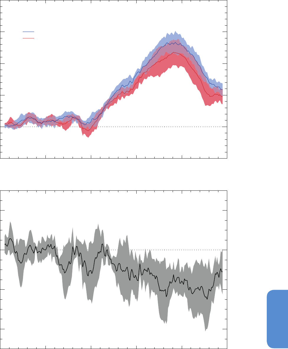
529
Carbon and Other Biogeochemical Cycles Chapter 6
6
1850 1900 1950 2000 2050 2100
Years
-5
0
5
10
15
20
(PgC yr
-1
)
RCP4.5 compatible fossil-fuel emissions
without climate feedback
with climate feedback
1850 1900 1950 2000 2050 2100
Years
-4
-2
0
2
(PgC yr
-1
)
Difference between simulations with and without feedbacks
Figure 6.27 | Compatible fossil fuel emissions for the RCP4.5 scenario (top) in the presence (red) and absence (blue) of the climate feedback on the carbon cycle, and the dif-
ference between them (bottom). Multi-model mean, 10-year smoothed values are shown, with 1 standard deviation shaded. This shows the impact of climate change on the
compatible fossil fuel CO
2
emissions to achieve the RCP4.5 CO
2
concentration pathway. Models used: Canadian Earth System Model 2 (CanESM2), Geophysical Fluid Dynamics
Laboratory–Earth System Model 2M (GFDL-ESM2M), Hadley Centre Global Environmental Model 2–Earth System (HadGEM2-ES), Institute Pierre Simon Laplace–Coupled Model
5A–Low Resolution (IPSL-CM5A-LR) and Model for Interdisciplinary Research On Climate–Earth System Model (MIROC–ESM).

530
Chapter 6 Carbon and Other Biogeochemical Cycles
6
Frequently Asked Questions
FAQ 6.1 | Could Rapid Release of Methane and Carbon Dioxide from Thawing Permafrost or
Ocean Warming Substantially Increase Warming?
Permafrost is permanently frozen ground, mainly found in the high latitudes of the Arctic. Permafrost, including
the sub-sea permafrost on the shallow shelves of the Arctic Ocean, contains old organic carbon deposits. Some are
relicts from the last glaciation, and hold at least twice the amount of carbon currently present in the atmosphere as
carbon dioxide (CO
2
). Should a sizeable fraction of this carbon be released as methane and CO
2
, it would increase
atmospheric concentrations, which would lead to higher atmospheric temperatures. That in turn would cause yet
more methane and CO
2
to be released, creating a positive feedback, which would further amplify global warming.
The Arctic domain presently represents a net sink of CO
2
—sequestering around 0.4 ± 0.4 PgC yr
–1
in growing vegeta-
tion representing about 10% of the current global land sink. It is also a modest source of methane (CH
4
): between
15 and 50 Tg(CH
4
) yr
–1
are emitted mostly from seasonally unfrozen wetlands corresponding to about 10% of the
global wetland methane source. There is no clear evidence yet that thawing contributes significantly to the current
global budgets of these two greenhouse gases. However, under sustained Arctic warming, modelling studies and
expert judgments indicate with medium agreement that a potential combined release totalling up to 350 PgC as
CO
2
equivalent could occur by the year 2100.
Permafrost soils on land, and in ocean shelves, con-
tain large pools of organic carbon, which must be
thawed and decomposed by microbes before it can
be released—mostly as CO
2
. Where oxygen is limited,
as in waterlogged soils, some microbes also produce
methane.
On land, permafrost is overlain by a surface ‘active
layer’, which thaws during summer and forms part of
the tundra ecosystem. If spring and summer tempera-
tures become warmer on average, the active layer will
thicken, making more organic carbon available for
microbial decomposition. However, warmer summers
would also result in greater uptake of carbon diox-
ide by Arctic vegetation through photosynthesis. That
means the net Arctic carbon balance is a delicate one
between enhanced uptake and enhanced release of
carbon.
Hydrological conditions during the summer thaw are
also important. The melting of bodies of excess ground
ice may create standing water conditions in pools and
lakes, where lack of oxygen will induce methane pro-
duction. The complexity of Arctic landscapes under
climate warming means we have low confidence in
which of these different processes might dominate on
a regional scale. Heat diffusion and permafrost melt-
ing takes time—in fact, the deeper Arctic permafrost can be seen as a relict of the last glaciation, which is still slowly
eroding—so any significant loss of permafrost soil carbon will happen over long time scales.
Given enough oxygen, decomposition of organic matter in soil is accompanied by the release of heat by microbes
(similar to compost), which, during summer, might stimulate further permafrost thaw. Depending on carbon and
ice content of the permafrost, and the hydrological regime, this mechanism could, under warming, trigger rela-
tively fast local permafrost degradation. (continued on next page)
CO
2
uptake
24-100 TgC yr
-1
CH
4
outgassing
1-12 TgCH
4
yr
-1
CH
4
from lakes and bogs
31-100 TgCH
4
yr
-1
CO
2
uptake by
land vegetation
0.3-0.6 PgC yr
-1
Permafrost soils
1500-1850 PgC
CH
4
hydrates
3-130 PgCH
4
Arctic ocean shelves
and shelf slopes
CH
4
hydrates 2-65 PgCH
4
Arctic ocean floor
CH
4
hydrates
30-170 PgCH
4
Flux to sediment
~2 TgC yr
-1
Flux to sediment
~8 TgC yr
-1
C transport by rivers
~80 TgC yr
-1
FAQ 6.1, Figure 1 | A simplified graph of current major carbon pools and flows
in the Arctic domain, including permafrost on land, continental shelves and ocean.
(Adapted from McGuire et al., 2009; and Tarnocai et al., 2009.) TgC = 10
12
gC,
and PgC = 10
15
gC.

531
Carbon and Other Biogeochemical Cycles Chapter 6
6
Modelling studies of permafrost dynamics and greenhouse gas emissions indicate a relatively slow positive feed-
back, on time scales of hundreds of years. Until the year 2100, up to 250 PgC could be released as CO
2
, and up to
5 Pg as CH
4
. Given methane’s stronger greenhouse warming potential, that corresponds to a further 100 PgC of
equivalent CO
2
released until the year 2100. These amounts are similar in magnitude to other biogeochemical feed-
backs, for example, the additional CO
2
released by the global warming of terrestrial soils. However, current models
do not include the full complexity of Arctic processes that occur when permafrost thaws, such as the formation of
lakes and ponds.
Methane hydrates are another form of frozen carbon, occurring in deep permafrost soils, ocean shelves, shelf slopes
and deeper ocean bottom sediments. They consist of methane and water molecule clusters, which are only stable in
a specific window of low temperatures and high pressures. On land and in the ocean, most of these hydrates origi-
nate from marine or terrestrial biogenic carbon, decomposed in the absence of oxygen and trapped in an aquatic
environment under suitable temperature–pressure conditions.
Any warming of permafrost soils, ocean waters and sediments and/or changes in pressure could destabilise those
hydrates, releasing their CH
4
to the ocean. During larger, more sporadic releases, a fraction of that CH
4
might also
be outgassed to the atmosphere. There is a large pool of these hydrates: in the Arctic alone, the amount of CH
4
stored as hydrates could be more than 10 times greater than the CH
4
presently in the global atmosphere.
Like permafrost thawing, liberating hydrates on land is a slow process, taking decades to centuries. The deeper
ocean regions and bottom sediments will take still longer—between centuries and millennia to warm enough to
destabilise the hydrates within them. Furthermore, methane released in deeper waters has to reach the surface
and atmosphere before it can become climatically active, but most is expected to be consumed by microorganisms
before it gets there. Only the CH
4
from hydrates in shallow shelves, such as in the Arctic Ocean north of Eastern
Siberia, may actually reach the atmosphere to have a climate impact.
Several recent studies have documented locally significant CH
4
emissions over the Arctic Siberian shelf and from
Siberian lakes. How much of this CH
4
originates from decomposing organic carbon or from destabilizing hydrates is
not known. There is also no evidence available to determine whether these sources have been stimulated by recent
regional warming, or whether they have always existed—it may be possible that these CH
4
seepages have been
present since the last deglaciation. In any event, these sources make a very small contribution to the global CH
4
budget—less than 5%. This is also confirmed by atmospheric methane concentration observations, which do not
show any substantial increases over the Arctic.
However modelling studies and expert judgment indicate that CH
4
and CO
2
emissions will increase under Arctic
warming, and that they will provide a positive climate feedback. Over centuries, this feedback will be moderate: of
a magnitude similar to other climate–terrestrial ecosystem feedbacks. Over millennia and longer, however, CO
2
and
CH
4
releases from permafrost and shelves/shelf slopes are much more important, because of the large carbon and
methane hydrate pools involved.
where Ω
A
= [Ca
+2
][CO
3
2–
]/K
sp
, where K
sp
is the solubility product for
the metastable form of CaCO
3
known as aragonite; a value of Ω
A
<1
thus indicates aragonite undersaturation). This aragonite undersatura-
tion in surface waters is reached before the end of the 21st century in
the Southern Ocean as highlighted in AR4, but occurs sooner and is
more intense in the Arctic (Steinacher et al., 2009). Ten percent of Arctic
surface waters are projected to become undersaturated when atmo-
spheric CO
2
reaches 428 ppm (by 2025 under all IPCC SRES scenarios).
That proportion increases to 50% when atmospheric CO
2
reaches 534
ppm (Steinacher et al., 2009). By 2100 under the A2 scenario, much of
the Arctic surface is projected to become undersaturated with respect
to calcite (Feely et al., 2009). Surface waters would then be corrosive
to all CaCO
3
minerals. These general trends are confirmed by the latest
projections from the CMIP5 Earth System models (Figure 6.28 and
6.29). Between 1986–2005 and 2081–2100, decrease in global-mean
surface pH is 0.065 (0.06 to 0.07) for RCP2.6, 0.145 (0.14 to 0.15) for
RCP4.5, 0.203 (0.20 to 0.21) for RCP6.0 and 0.31 (0.30 to 0.32) for
RCP8.5 (range from CMIP5 models spread).
Surface CaCO
3
saturation also varies seasonally, particularly in the
high latitudes, where observed saturation is higher in summer and
lower in winter (Feely et al., 1988; Merico et al., 2006; Findlay et al.,
FAQ 6.1 (continued)
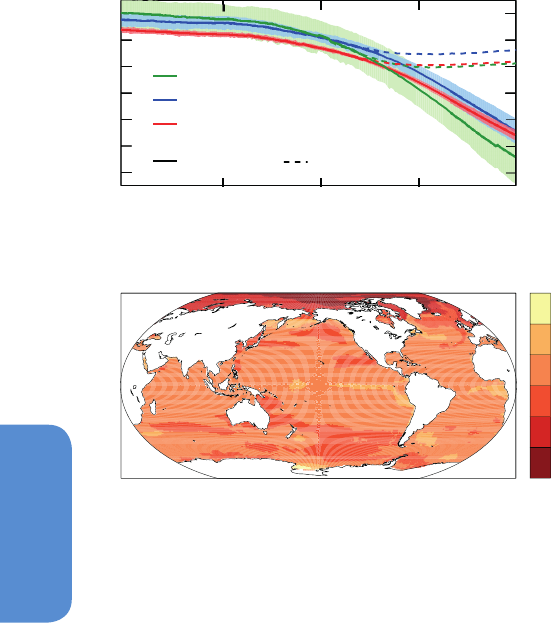
532
Chapter 6 Carbon and Other Biogeochemical Cycles
6
a. Surface pH
b. Surface pH in 2090s (RCP8.5, changes from 1990s)
1900 1950 2000 2050 2100
7.6
7.7
7.8
7.9
8.0
8.1
8.2
-0.2
-0.3
-0.4
-0.5
Arctic (>70°N)
S.Ocean (<60°S)
Tropics (20°S-20°N)
RCP8.5
RCP2.6
2008). Future projections using ocean carbon cycle models indicate
that undersaturated conditions will be reached first in winter (Orr et
al., 2005). In the Southern Ocean, it is projected that wintertime under-
saturation with respect to aragonite will begin when atmospheric
CO
2
will reach 450 ppm, within 1-3 decades, which is about 100 ppm
sooner (~30 years under the IS92a scenario) than for the annual mean
undersaturation (McNeil and Matear, 2008). As well, aragonite under-
saturation will be first reached during wintertime in parts (10%) of
the Arctic when atmospheric CO
2
will reach 410 ppm, within a decade
(Steinacher et al., 2009). Then, aragonite undersaturation will become
widespread in these regions at atmospheric CO
2
levels of 500–600
ppm (Figure 6.28).
Although projected changes in pH are generally largest at the surface,
the greatest pH changes in the subtropics occur between 200 and 300
m where subsurface increased loads of anthropogenic CO
2
are similar
to surface changes but the carbonate buffering capacity is lower (Orr,
2011). This more intense projected subsurface pH reduction is consis-
tent with the observed subsurface changes in pH in the subtropical
North Pacific (Dore et al., 2009; Byrne et al., 2010; Ishii et al., 2011). As
Figure 6.28 | Projected ocean acidification from 11 CMIP5 Earth System Models under
RCP8.5 (other RCP scenarios have also been run with the CMIP5 models): (a) Time
series of surface pH shown as the mean (solid line) and range of models (filled), given
as area-weighted averages over the Arctic Ocean (green), the tropical oceans (red) and
the Southern Ocean (blue). (b) Maps of the median model’s change in surface pH from
1850 to 2100. Panel (a) also includes mean model results from RCP2.6 (dashed lines).
Over most of the ocean, gridded data products of carbonate system variables (Key et
al., 2004) are used to correct each model for its present-day bias by subtracting the
model-data difference at each grid cell following (Orr et al., 2005). Where gridded data
products are unavailable (Arctic Ocean, all marginal seas, and the ocean near Indone-
sia), the results are shown without bias correction. The bias correction reduces the range
of model projections by up to a factor of 4, e.g., in panel (a) compare the large range
of model projections for the Arctic (without bias correction) to the smaller range in the
Southern Ocean (with bias correction).
subsurface saturation states decline, the horizon separating undersatu-
rated waters below from supersaturated waters above is projected to
move upward (shoal). By 2100 under the RCP8.5 scenario, the median
projection from 11 CMIP5 models is that this interface (aragonite sat-
uration horizon) will shoal from 200 m up to 40 m in the subarctic
Pacific, from 1000 m up to the surface in the Southern Ocean, and from
2850 m to 150 m in the North Atlantic (Figure 6.29), consistent with
results from previous model comparison (Orr et al., 2005; Orr, 2011).
Under the SRES A2 scenario, the volume of ocean with supersaturated
waters is projected to decline from 42% in the preindustrial Era to
25% in 2100 (Steinacher et al., 2009). Yet even if atmospheric CO
2
does
not go above 450 ppm, most of the deep ocean volume is projected
to become undersaturated with respect to both aragonite and calcite
after several centuries (Caldeira and Wickett, 2005). Nonetheless, the
most recent projections under all RCPs scenarios but RCP8.5 illustrate
that limiting atmospheric CO
2
will greatly reduce the level of ocean
acidification that will be experienced (Joos et al., 2011).
In the open ocean, future reductions in surface ocean pH and CaCO
3
(calcite and aragonite) saturation states are controlled mostly by the
invasion of anthropogenic carbon. Other effects due to future climate
change counteract less than 10% of the reductions in CaCO
3
satura-
tion induced by the invasion of anthropogenic carbon (Orr et al., 2005;
McNeil and Matear, 2006; Cao et al., 2007). Warming dominates other
effects from climate-change by reducing CO
2
solubility and thus by
enhancing [CO
3
2–
]. An exception is the Arctic Ocean where reductions
in pH and CaCO
3
saturation states are projected to be exacerbated
by effects from increased freshwater input due to sea ice melt, more
precipitation, and greater air–sea CO
2
fluxes due to less sea ice cover
(Steinacher et al., 2009; Yamamoto et al., 2012). The projected effect
of freshening is consistent with current observations of lower satura-
tion states and lower pH values near river mouths and in areas under
substantial fresh-water influence (Salisbury et al., 2008; Chierici and
Fransson, 2009; Yamamoto-Kawai et al., 2009).
Regional ocean carbon cycle models project that some nearshore sys-
tems are also highly vulnerable to future pH decrease. In the California
Current System, an eastern boundary upwelling system, observations
and model results show that strong seasonal upwelling of carbon-
rich waters (Feely et al., 2008) renders surface waters as vulnerable
to future ocean acidification as those in the Southern Ocean (Gruber
et al., 2012). In the Northwestern European Shelf Seas, large spatio-
temporal variability is enhanced by local effects from river input and
organic matter degradation, exacerbating acidification from anthropo-
genic CO
2
invasion (Artioli et al., 2012). In the Gulf of Mexico and East
China Sea, coastal eutrophication, another anthropogenic perturba-
tion, has been shown to enhance subsurface acidification as additional
respired carbon accumulates at depth (Cai et al., 2011).
6.4.5 Future Ocean Oxygen Depletion
It is very likely that global warming will lead to declines in dissolved O
2
in the ocean interior through warming-induced reduction in O
2
solubil-
ity and increased ocean stratification. This will have implications for
nutrient and carbon cycling, ocean productivity and marine habitats
(Keeling et al., 2010).
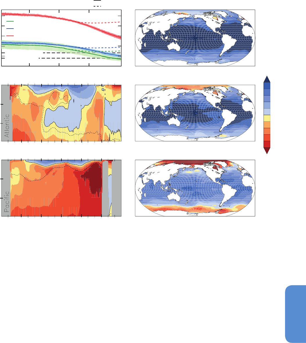
533
Carbon and Other Biogeochemical Cycles Chapter 6
6
a. Surface CO
3
2-
(μmol kg
-1
)
1900 1950 2000 2050 2100
Arctic (>70°N)
S.Ocean (<60°S)
Tropics (20°S-20°N)
RCP8.5
RCP2.6
0
100
200
Calcite Saturation
Aragonite Saturation
b. Surface Ω
Aragonite
RCP8.5 2010
0
1000
2000
3000
0
1000
2000
3000
Depth (m)
0° 30°N 60°N 90°N90°S 60°S 30°S
d. Surface Ω
Aragonite
RCP8.5 2050
f. Surface Ω
Aragonite
RCP8.5 2100
e. Ω
Aragonite
RCP8.5 2100
c. Ω
Aragonite
RCP8.5 2100
0.5
1
2
3
2.5
1.2
1.5
0.6
0.7
0.8
0.9
Figure 6.29 | Projected aragonite saturation state from 11 CMIP5 Earth System Models under RCP8.5 scenario: (a) time series of surface carbonate ion concentration shown as
the mean (solid line) and range of models (filled), given as area-weighted averages over the Arctic Ocean (green), the tropical oceans (red), and the Southern Ocean (blue); maps
of the median model’s surface Ω
A
in (b) 2010, (d) 2050 and (f) 2100; and zonal mean sections (latitude vs. depth) of Ω
A
in 2100 over the (c) Atlantic and (e) Pacific, while the ASH
is shown in 2010 (dotted line) as well as 2100 (solid line). Panel (a) also includes mean model results from RCP2.6 (dashed lines). As for Figure 6.28, gridded data products of
carbonate system variables (Key et al., 2004) are used to correct each model for its present-day bias by subtracting the model-data difference at each grid cell following (Orr et al.,
2005). Where gridded data products are unavailable (Arctic Ocean, all marginal seas, and the ocean near Indonesia), results are shown without bias correction.
Future changes in dissolved O
2
have been investigated using models of
various complexity (see references in Table 6.13). The global ocean dis-
solved oxygen will decline significantly under future scenarios (Cocco
et al., 2013). Simulated declines in mean dissolved O
2
concentration for
the global ocean range from 6 to 12 μmol kg
–1
by the year 2100 (Table
6.13), with a projection of 3 to 4 μmol kg
–1
in one model with low cli-
mate sensitivity (Frölicher et al., 2009). This general trend is confirmed
by the latest projections from the CMIP5 Earth System models, with
reductions in mean dissolved O
2
concentrations from 1.5 to 4% (2.5
to 6.5 μmol kg
–1
) in 2090s relative to 1990s for all RCPs (Figure 6.30a).
Most modelling studies (Table 6.13) explain the global decline in dis-
solved oxygen by enhanced surface ocean stratification leading to
reductions in convective mixing and deep water formation and by a
contribution of 18 to 50% from ocean warming-induced reduction in
solubility. These two effects are in part compensated by a small increase
in O
2
concentration from projected reductions in biological export
production production (Bopp et al., 2001; Steinacher et al., 2010) or
changes in ventilation age of the tropical thermocline (Gnanadesikan
et al., 2007). The largest regional decreases in oxygen concentration
(~20 to 100 μmol kg
–1
) are projected for the intermediate (200 to 400
m) to deep waters of the North Atlantic, North Pacific and Southern
Ocean for 2100 (Plattner et al., 2002; Matear and Hirst, 2003; Frölicher
et al., 2009; Matear et al., 2010; Cocco et al., 2013), which is confirmed
by the latest CMIP5 projections (Figure 6.30c and 6.30d).
It is as likely as not that the extent of open-ocean hypoxic (dissolved
oxygen <60 to 80 μmol kg
–1
) and suboxic (dissolved oxygen <5 μmol
kg
–1
) waters will increase in the coming decades. Most models show
even some increase in oxygen in most O
2
-poor waters and thus a slight
decrease in the extent of suboxic waters under the SRES-A2 scenario
(Cocco et al., 2013), as well as under RCP8.5 scenario (see the model-

534
Chapter 6 Carbon and Other Biogeochemical Cycles
6
Study
Ocean Carbon
Cycle Model
Forcing
Mean [O
2
] Decrease
(μmol kg
–1
)
a,b
Solubility
Contribution (%)
Sarmiento et al. (1998) GFDL 7
c
Matear et al. (2000) CSIRO IS92a 18
Plattner et al. (2002) Bern 2D SRES A1 12 35
Bopp et al. (2002) IPSL SRES A2
d
4 25
Matear and Hirst (2003) CSIRO IS92a 9 26
Schmittner et al. (2008) UVic SRES A2 9
Oschlies et al. (2008) UVic SRES A2 9
UVic-variable C:N SRES A2 12
Frölicher et al. (2009) NCAR CSM1.4-CCCM SRES A2 4 50
SRES B1 3
Shaffer et al. (2009) DCESS SRES A2 10
e
Table 6.13 | Model configuration and projections for global marine O
2
depletion by 2100 (adapted from Keeling et al. (2010).
Notes:
a
Assuming a total ocean mass of 1.48 × 10
21
kg.
b
Relative to pre-industrial baseline in 1750.
c
Model simulation ends at 2065.
d
Radiative forcing of non-CO
2
GHGs is excluded from this simulation.
e
For simulations with reduced ocean exchange.
CCCM = Coupled-Climate-Carbon Model; CSIRO = Commonwealth Scientific and Industrial Research Organisation; DCESS = Danish Center for Earth System Science; GFDL = Geophysical Fluid
Dynamics Laboratory; IPSL = Institute Pierre Simon Laplace; NCAR = National Center for Atmospheric Research; IS92 = IPCC scenarios for 1992; SRES = Special Report on Emission Scenarios; UVic
= University of Victoria.
mean increase of sub-surface O
2
in large parts of the tropical Indian
and Atlantic Oceans, Figure 6.30d). This rise in oxygen in most sub-
oxic waters has been shown to be caused in one model study by an
increased supply of oxygen due to lateral diffusion (Gnanadesikan
et al., 2012). Given limitations of global ocean models in simulating
today’s O
2
distribution (Cocco et al., 2013), as well as reproducing the
measured changes in O
2
concentrations over the past 50 years (see
Chapter 3, and Stramma et al., 2012), the model projections are uncer-
tain, especially concerning the evolution of O
2
in and around oxygen
minimum zones.
A number of biogeochemical ocean carbon cycle feedbacks, not yet
included in most marine biogeochemical models (including CMIP5
models, see Section 6.3.2.5.6), could also impact future trends of ocean
deoxygenation. For example, model experiments which include a pCO
2
-
sensitive C:N drawdown in primary production, as suggested by some
mesocosm experiments (Riebesell et al., 2007), project future increases
of up to 50% in the volume of the suboxic waters by 2100 (Oschlies
et al., 2008; Tagliabue et al., 2011). In addition, future marine hypoxia
could be amplified by changes in the CaCO
3
to organic matter ‘rain
ratio’ in response to rising pCO
2
(Hofmann and Schellnhuber, 2009).
Reduction in biogenic calcification due to ocean acidification would
weaken the strength of CaCO
3
mineral ballasting effect, which could
lead organic material to be remineralized at a shallower depth exacer-
bating the future expansion of shallow hypoxic waters.
The modeled estimates do not take into account processes that are
specific to the coastal ocean and may amplify deoxygenation. Recent
observations for the period 1976–2000 have shown that dissolved O
2
concentrations have declined at a faster rate in the coastal ocean (–0.28
μmol kg
–1
yr
–1
) than the open ocean (–0.02 μmol kg
–1
y
–1
, and a faster
rate than in the period 1951–1975, indicating a worsening of hypoxia
(Gilbert et al., 2010). Hypoxia in the shallow coastal ocean (apart from
continental shelves in Eastern Boundary Upwelling Systems) is largely
eutrophication driven and is controlled by the anthropogenic flux of
nutrients (N and P) and organic matter from rivers. If continued indus-
trialisation and intensification of agriculture yield larger nutrient loads
in the future, eutrophication should intensify (Rabalais et al., 2010),
and further increase the coastal ocean deoxygenation.
On longer time scales beyond 2100, ocean deoxygenation is projected
to increase with some models simulating a tripling in the volume of
suboxic waters by 2500 (Schmittner et al., 2008). Ocean deoxygen-
ation and further expansion of suboxic waters could persist on millen-
nial time scales, with average dissolved O
2
concentrations projected
to reach minima of up to 56 μmol kg
–1
below pre-industrial levels
in experiments with high CO
2
emissions and high climate sensitivity
(Shaffer et al., 2009).
A potential expansion of hypoxic or suboxic water over large parts
of the ocean is likely to impact the marine cycling of important nutri-
ents, particularly nitrogen. The intensification of low oxygen waters has
been suggested to lead to increases in water column denitrification
and N
2
O emissions (e.g., Codispoti, 2010; Naqvi et al., 2010). Recent
works, however, suggest that oceanic N
2
O production is dominated
by nitrification with a contribution of 7% by denitrification (Freing et
al., 2012), Figure 6.4c) and that ocean deoxygenation in response to
anthropogenic climate change could leave N
2
O production relatively
unchanged (Bianchi et al., 2012).
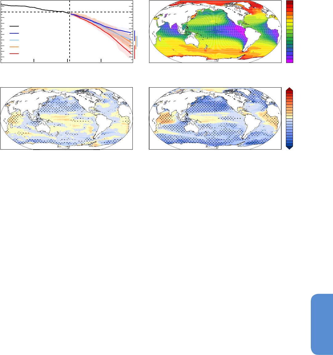
535
Carbon and Other Biogeochemical Cycles Chapter 6
6
a. Ocean oxygen content change (%) b. Oxygen concentrations (200-600m) 1990s
c. 2090s, changes from 1990s RCP2.6
d. 2090s, changes from 1990s RCP8.5
(mmol m
-3
)
280
240
80
40
0
200
160
120
320
40
30
-10
-20
-30
20
10
0
50
-40
-50
RCP2.6
RCP4.5
RCP6.0
RCP8.5
1900 1950 2000 2050 2100
-4
-3
-2
-1
0
1
Historical
Figure 6.30 | (a) Simulated changes in dissolved O
2
(mean and model range as shading) relative to 1990s for RCP2.6, RCP4.5, RCP6.0 and RCP8.5. (b) Multi-model mean dis-
solved O
2
(μmol m
–3
) in the main thermocline (200 to 600 m depth average) for the 1990s, and changes in 2090s relative to 1990s for RCP2.6 (c) and RCP8.5 (d). To indicate
consistency in the sign of change, regions are stippled where at least 80% of models agree on the sign of the mean change. These diagnostics are detailed in Cocco et al. (2013)
in a previous model intercomparison using the SRES-A2 scenario and have been applied to CMIP5 models here. Models used: Community Earth System Model 1–Biogeochemical
(CESM1-BGC), Geophysical Fluid Dynamics Laboratory–Earth System Model 2G (GFDL-ESM2G), Geophysical Fluid Dynamics Laboratory–Earth System Model 2M (GFDL-ESM2M),
Hadley Centre Global Environmental Model 2–Earth System (HadGEM2-ES), Institute Pierre Simon Laplace–Coupled Model 5A–Low Resolution (IPSL-CM5A-LR), Institute Pierre
Simon Laplace–Coupled Model 5A–Medium Resolution (IPSL-CM5A-MR), Max Planck Institute–Earth System Model–Low Resolution (MPI-ESM-LR), Max Planck Institute–Earth
System Model–Medium Resolution (MPI-ESM-MR), Norwegian Earth System Model 1 (Emissions capable) (NorESM1).
6.4.6 Future Trends in the Nitrogen Cycle and Impact
on Carbon Fluxes
6.4.6.1 Projections for Formation of Reactive Nitrogen by
Human Activity
Since the 1970s, food production, industrial activity and fossil fuel
combustion have resulted in the creation of more reactive nitrogen
(Nr) than natural terrestrial processes (Section 6.1; Box 6.2, Figure 1).
Building on the general description of the set of AR4 Special Report on
Emission (SRES) scenarios, Erisman et al. (2008) estimated anthropo-
genic nitrogen fertiliser consumption throughout the 21st century. Five
driving parameters (population growth, consumption of animal pro-
tein, agricultural efficiency improvement and additional biofuel pro-
duction) are used to project future nitrogen demands for four scenarios
(A1, B1, A2 and B2) (Figure 6.31). Assigning these drivers to these four
SRES scenarios, they estimated a production of Nr for agricultural use
of 90 to 190 TgN yr
–1
by 2100, a range that spans from slightly less to
almost twice as much current fertiliser consumption rates (Section 6.1,
Figure 6.4a, Figure 1 in Box 6.2).
Despite the uncertainties and the non-inclusion of many important
drivers, three of the scenarios generated by the Erisman et al. (2008)
model point towards an increase in future production of reactive
nitrogen. In particular, the A1 scenario which assumes a world with
rapid economic growth, a global population that peaks mid-century
and rapid introduction of new and more efficient technologies ends
up as the potentially largest contributor to nitrogen use, as a result of
large amounts of biofuels required and the fertiliser used to produce
it. This increase in nitrogen use is assumed to be largely in line with
the RCP2.6 scenario, where it appears to have rather limited adverse
effects like increasing N
2
O emissions (van Vuuren et al., 2011).
N
2
O emissions are projected to increase from increased anthropogen-
ic Nr production. It is thus likely that N
2
O emissions from soils will
increase due to the increased demand for feed/food and the reliance of
agriculture on nitrogen fertilisers. This is illustrated by the comparison
of emissions from 1900 to those in 2000 and 2050, using the IAM
IMAGE model that served to define the RCP2.6 pathway (Figure 6.32).
The anthropogenic N
2
O emission map IN 2050 shown in Figure 6.32 is
established from the RCP4.5 scenario; the RCP8.5 and RCP6 scenarios
have much higher emissions, and RCP2.6 much lower (van Vuuren et
al., 2011). A spatially explicit inventory of soil nitrogen budgets in live-
stock and crop production systems using the IMAGE model (Bouwman
et al., 2011) shows that between 1900 and 1950, the global soil Nr
budget surplus almost doubled to 36 TgN yr
–1
, and further increased to
138 TgN yr
–1
between 1950 and 2000. The IMAGE model scenario from
Bouwman et al. (2011) shown in Figure 6.32 portrays a world with a
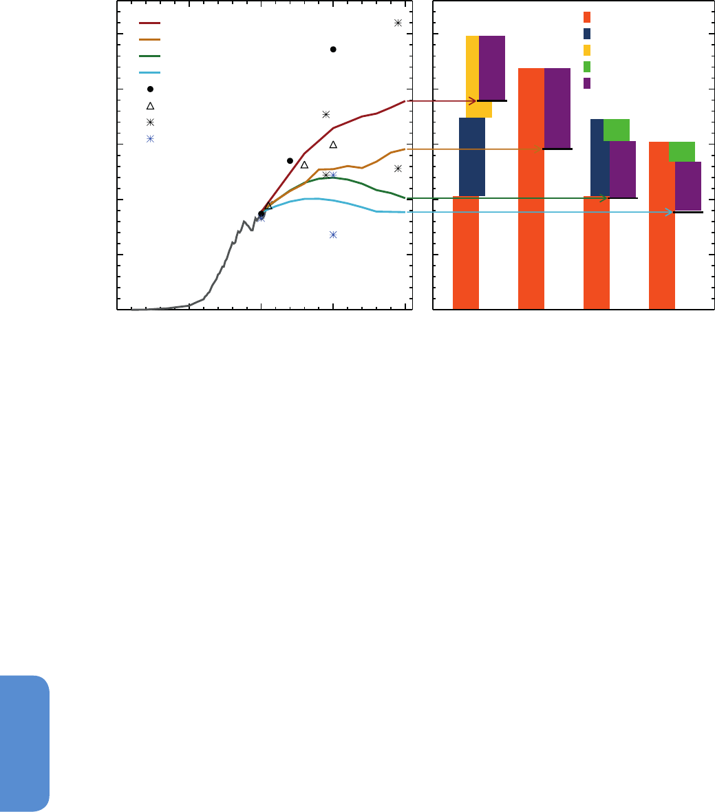
536
Chapter 6 Carbon and Other Biogeochemical Cycles
6
1900 1950 2000 2050 2100
Year
0
50
100
150
200
250
Global fertilizer Nr demand (Tg N yr
-1
)
SRES A1 + biofuel
SRES A2
SRES B1
SRES B2
Tilman et al. 2001
FAO 2012
Bodirsky et al. 2012
Bouwman et al. 2009
A1 A2 B1 B2
0
50
100
150
200
250
population
food equity
biofuels
diet optimization
efficiency increase
further increasing global crop production (+82% for 2000–2050) and
livestock production (+115%). Despite the assumed rapid increase
in nitrogen use efficiency in crop (+35%) and livestock (+35%) pro-
duction, global agricultural Nr surpluses are projected to continue to
increase (+23%), and associated emissions of N
2
O to triple compared
to 1900 levels.
Regional to global scale model simulations suggest a strong effect
of climate variability on interannual variability of land N
2
O emissions
(Tian et al., 2010; Zaehle et al., 2011; Xu-Ri et al., 2012). Kesik et al.
(2006) found for European forests that higher temperatures and lower
soil moisture will decrease future N
2
O emissions under scenarios of
climate change, despite local increases of emission rates by up to 20%.
Xu-Ri et al. (2012) show that local climate trends result in a spatially
diverse pattern of increases and decreases of N
2
O emissions, which
globally integrated result in a net climate response of N
2
O emissions
of 1 TgN yr
–1
per 1°C of land temperature warming. Using a further
development of this model, Stocker et al. (2013) estimate increases in
terrestrial N
2
O from a pre-industrial terrestrial source of 6.9 TgN (N
2
O)
yr
–1
to 9.8 to 11.1 TgN (N
2
O) yr
–1
(RCP 2.6) and 14.2 to 17.0 TgN (N
2
O)
yr
–1
(RCP 8.5) by 2100. Of these increases, 1.1 to 2.4 TgN (N
2
O) yr
–1
(RCP 2.6) or 4.7 to 7.7 TgN (N
2
O) yr
–1
(RCP 8.5) are due to the inter-
acting effects of climate and CO
2
on N
2
O emissions from natural and
agricultural ecosystems. An independent modelling study suggested a
climate change related increase of N
2
O emissions between 1860 and
2100 by 3.1 TgN (N
2
O) yr
–1
for the A2 SRES scenario (Zaehle, 2013)
implying a slightly lower sensitivity of soil N
2
O emissions to climate of
0.5 TgN (N
2
O) yr
–1
per 1°C warming. While the present-day contribu-
tion of these climate-mediated effects on the radiative forcing from
N
2
O is likely to be small (0.016 W m
–2
°C
–1
; Zaehle and Dalmonech,
Figure 6.31 | Global nitrogen fertiliser consumption scenarios (left) and the impact of individual drivers on 2100 consumption (right). This resulting consumption is always
the sum (denoted at the end points of the respective arrows) of elements increasing as well as decreasing nitrogen consumption. Other relevant estimates are presented for
comparison. The A1, B1, A2 and B2 scenarios draw from the assumptions of the IPCC Special Report on Emission Scenarios (SRES) emission scenario storylines as explained in
Erisman et al. (2008).
2011). Modelling results (Stocker et al., 2013) suggest that the climate
and CO
2
-related amplification of terrestrial N
2
O emissions imply a
larger feedback of 0.03 to 0.05 W m
–2
°C
–1
by 2100.
With the continuing increases in the formation of Nr from anthropo-
genic activities will come increased Nr emissions and distribution of
Nr by waters and the atmosphere. For the atmosphere, the main driver
of future global nitrogen deposition is the emission trajectories of NO
y
and NH
3
. For all RCP scenarios except RCP2.6, nitrogen deposition is
projected to remain relatively constant globally although there is a
projected increase in NH
x
deposition and decrease in NO
y
deposition.
On a regional basis, future decreases of NH
x
and NOx are projected
in North America and northern Europe, and increases in Asia (Figure
6.33). Spatially, projected changes in total nitrogen deposition driven
primarily by increases in NH
x
emissions occur over large regions of the
world for all RCPs, with generally the largest in RCP8.5 and the small-
est in RCP2.6 (Figure 6.33) (Supplementary Material has RCP4.5 and
RCP6.0). Previous IPCC scenarios (SRES A2 or IS92a) project a near
doubling of atmospheric nitrogen deposition over some world biodi-
versity hotspots with half of these hotspots subjected to deposition
rates greater than 15 kgN ha
–1
yr
–1
(critical load threshold value) over
at least 10% of their total area (Dentener et al., 2005; Phoenix et al.,
2006; Bleeker et al., 2011).
Large uncertainties remain in our understanding and modelling of
changes in Nr emissions, atmospheric transport and deposition pro-
cesses, lead to low confidence in the projection of future Nr deposition
fluxes, particularly in regions remote from anthropogenic emissions
(Dentener et al., 2006). The large spread between atmospheric GCM
models associated with precipitation projections confounds extraction
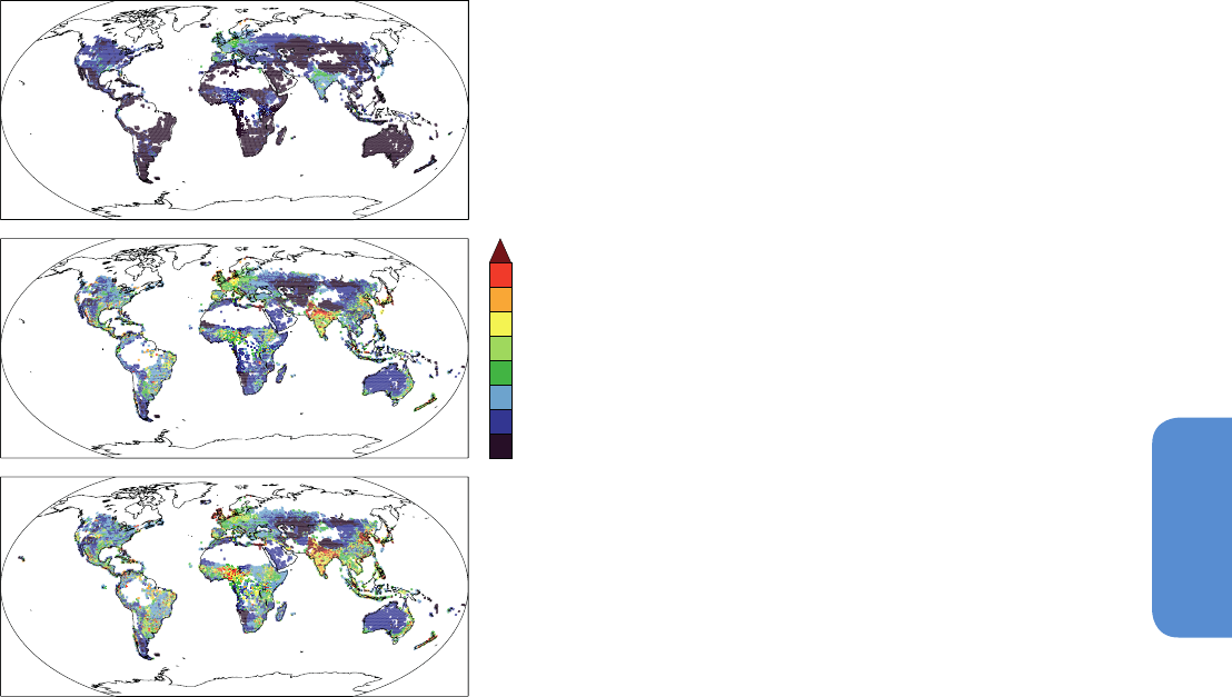
537
Carbon and Other Biogeochemical Cycles Chapter 6
6
Figure 6.32 | N
2
O emissions in 1900, 2000 and projected to 2050 (Bouwman et al.,
2011). This spatially explicit soil nutrient budget and nitrogen gas emission scenario
was elaborated with the Integrated Model to Assess the Global Environment (IMAGE)
model on the basis of the International Assessment of Agricultural Knowledge, Science
and Technology for Development (IAASTD) baseline scenario (McIntyre et al., 2009).
of a climate signal in deposition projections (Langner et al., 2005;
Hedegaard et al., 2008).
6.4.6.2. Projected Changes in Sulphur Deposition
Given the tight coupling between the atmospheric nitrogen and sul-
phur cycles, and the impact on climate (Section 7.3) this Chapter also
presents scenarios for sulphur deposition. Deposition of SO
x
is pro-
jected to decrease in all RCP pathways (Figures 6.33 and 6.34). By
contrast, scenarios established prior to RCPs indicated decreases of
sulphur deposition in North America and Europe, but increases in South
America, Africa, South and East Asia (Dentener et al., 2006; Tagaris et
al., 2008). In all RCPs, sulphur deposition is lower by 2100 than in 2000
in all regions, with the largest decreases in North America, Europe and
Asia (RCP2.6 and RCP 8.5 are seen in Figure 6.34; RCP4.5 and RCP6.0
are in the Supplementary Material) (Lamarque et al., 2011). Future hot
spots of deposition are still evident in East and South East Asia, espe-
cially for RCP6.0.
Projected future increase of Nr input into terrestrial ecosystems also
yields increased flux of Nr from rivers into coastal systems. As illus-
trated by the Global NEWS 2 model for 2050, by the base year 2000,
N
2
O emissions (kgN km
-2
y
-1
)
a. 1900
b. 2000
4
3
0
2
1
c. 2050
the discharge of dissolved inorganic nitrogen (DIN) to marine coastal
waters was >500 kg N km
–2
of watershed area for most watershed
systems downstream of either high population or extensive agricul-
tural activity (Mayorga et al., 2010; Seitzinger et al., 2010). Additional
information and the supporting figure are found in the Supplementary
Material.
6.4.6.3 Impact of Future Changes in Reactive Nitrogen on
Carbon Uptake and Storage
Anthropogenic Nr addition and natural nitrogen-cycle responses to
global changes will have an important impact on the global carbon
cycle. As a principal nutrient for plant growth, nitrogen can both limit
future carbon uptake and stimulate it depending on changes in Nr
availability. A range of global terrestrial carbon cycle models have
been developed since AR4 that integrate nitrogen dynamics into the
simulation of land carbon cycling (Thornton et al., 2007; Wang et al.,
2007, 2010a; Sokolov et al., 2008; Xu-Ri and Prentice, 2008; Churkina
et al., 2009; Jain et al., 2009; Fisher et al., 2010; Gerber et al., 2010;
Zaehle and Friend, 2010; Esser et al., 2011). However, only two ESMs in
CMIP5 (CESM1-BGC and NorESM1-ME) include a description of nitro-
gen–carbon interactions.
In response to climate warming, increased decomposition of soil
organic matter increases nitrogen mineralisation, (high confidence)
which can enhance Nr uptake and carbon storage by vegetation. Gen-
erally, higher C:N ratio in woody vegetation compared to C:N ratio
of soil organic matter causes increased ecosystem carbon storage as
increased Nr uptake shifts nitrogen from soil to vegetation (Melillo et
al., 2011). In two studies (Sokolov et al., 2008; Thornton et al., 2009),
this effect was strong enough to turn the carbon–climate interaction
into a small negative feedback, that is, an increased land CO
2
uptake
in response to climate warming (positive γ
L
values in Figure 6.20),
whereas in another study that described carbon–nitrogen interactions
(Zaehle et al., 2010b) the carbon–climate interaction was reduced but
remained positive, that is, decreased land CO
2
uptake in response to
climate change (negative γ
L
values in Figures 6.20, 6.21 and 6.22). The
two CMIP5 ESMs which include terrestrial carbon–nitrogen interac-
tions (Table 6.11) also simulate a small but positive climate–carbon
feedback.
Consistent with the observational evidence (Finzi et al., 2006; Palmroth
et al., 2006; Norby et al., 2010), modelling studies have shown a strong
effect of Nr availability in limiting the response of plant growth and
land carbon storage to elevated atmospheric CO
2
(e.g., Sokolov et al.,
2008; Thornton et al., 2009; Zaehle and Friend, 2010). These analyses
are affected by the projected future trajectories of anthropogenic Nr
deposition. The effects of Nr deposition counteract the nitrogen limita-
tion of CO
2
fertilisation (Churkina et al., 2009; Zaehle et al., 2010a).
Estimates of the total net carbon storage on land due to Nr deposition
between 1860 and 2100 range between 27 and 66 PgC (Thornton et
al., 2009; Zaehle et al., 2010a).
It is very likely that, at the global scale, nutrient limitation will reduce
the global land carbon storage projected by CMIP5 carbon-cycle only
models. Only two of the current CMIP5 ESM models explicitly con-
sider carbon–nitrogen interactions (CESM1-BGC and NorESM1-ME).
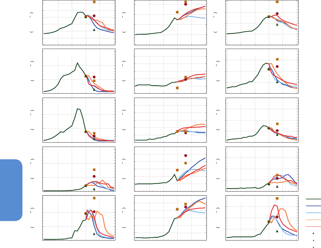
538
Chapter 6 Carbon and Other Biogeochemical Cycles
6
SO
x
Deposition NH
x
Deposition
NO
y
Deposition
0
20
40
60
80
100
120
TgSyr
1
World
0
20
40
60
80
TgNyr
1
World
0
20
40
60
80
TgNyr
1
World
0
5
10
15
TgSyr
1
North America
0
2
4
6
8
10
12
TgNyr
1
North America
0
2
4
6
8
TgNyr
1
North America
0
5
10
15
TgSyr
1
Europe
0
2
4
6
8
10
12
TgNyr
1
Europe
0
2
4
6
8
TgNyr
1
Europe
0
5
10
15
TgSyr
1
South Asia
0
2
4
6
8
10
12
TgNyr
1
South Asia
0
2
4
6
8
TgNyr
1
South Asia
1850 1900 1950 2000 2050 2100
0
5
10
15
Year
TgSyr
1
East Asia
1850 1900 1950 2000 2050 2100
0
2
4
6
8
10
12
Year
TgNyr
1
East Asia
1850 1900 1950 2000 2050 2100
0
2
4
6
8
Year
TgNyr
1
East Asia
Historical
RCP 2.6
RCP 4.5
RCP 6.0
RCP 8.0
CLE
A2
MFR
Figure 6.33 | Deposition of SO
x
(left, TgS yr
–1
), NH
x
(middle, TgN yr
–1
) and NO
y
(right, TgN yr
–1
) from 1850 to 2000 and projections of deposition to 2100 under the four RCP
emission scenarios (Lamarque et al., 2011; van Vuuren et al., 2011). Also shown are the 2030 scenarios using the SRES B1/A2 energy scenario with assumed current legislation and
maximum technically feasible air pollutant reduction controls (Dentener et al., 2006).
The effect of the nitrogen limitations on terrestrial carbon sequestra-
tion in the results of the other CMIP5 models may be approximated
by comparing the implicit Nr requirement given plausible ranges of
terrestrial C:N stoichiometry (Wang and Houlton, 2009) to plausible
increases in terrestrial Nr supply due to increased biological nitrogen
fixation (Wang and Houlton, 2009) and anthropogenic Nr deposition
(Figure 6.35). For the ensemble of CMIP5 projections under the RCP
8.5 scenario, this implies a lack of available nitrogen of 1.3 to 13.1
PgN which would reduce terrestrial C sequestration by an average of
137 PgC over the period 1860–2100, with a range of 41 to 273 PgC
among models. This represents an ensemble mean reduction in land
carbon sequestration of 55%, with a large spread across models (14
to 196%). Inferred reductions in ensemble-mean land carbon sink over
the same period for RCPs 6.0, 4.5 and 2.6 are 109, 117 and 85 PgC,
respectively. Between-model variation in these inferred reduced land
carbon sinks is similar for all RCPs, with ranges of 57 to 162 PgC, 38 to
208 PgC, and 32 to 171 PgC for RCPs 6.0, 4.5 and 2.6, respectively. The
influence of nutrient addition for agriculture and pasture management
is not addressed in this analysis. Results from the two CMIP5 models
with explicit carbon–nitrogen interactions show even lower land
carbon sequestration than obtained by this approximation method
(Figure 6.35). More models with explicit carbon–nitrogen interactions
are needed to understand between-model variation and construct an
ensemble response.
The positive effect on land carbon storage due to climate-increased
Nr mineralization is of comparable magnitude to the land carbon stor-
age increase associated with increased anthropogenic Nr deposition.
Models disagree, however, which of the two factors is more important,
with both effects dependent on the choice of scenario. Crucially, the
effect of nitrogen limitation on vegetation growth and carbon storage
under elevated CO
2
is the strongest effect of the natural and disturbed
nitrogen cycle on terrestrial carbon dynamics (Bonan and Levis, 2010;
Zaehle et al., 2010a). In consequence, the projected atmospheric CO
2
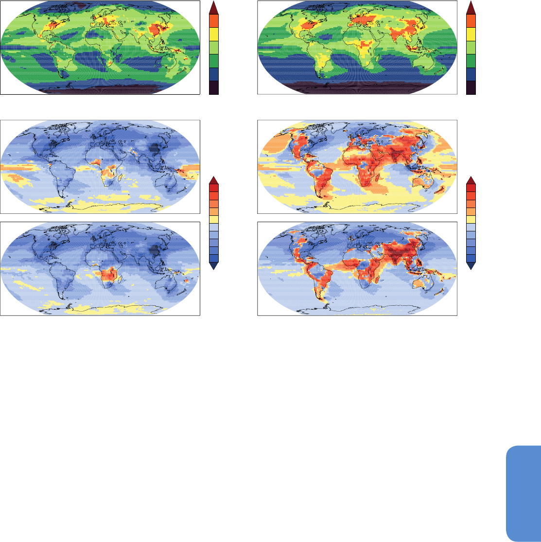
539
Carbon and Other Biogeochemical Cycles Chapter 6
6
Figure 6.34 | Spatial variability of nitrogen and SO
x
deposition in 1990s with projections to the 2090s (shown as difference relative to the 1990s), using the RCP2.6 and RCP8.5
scenarios, kgN km
–2
yr
–1
, adapted fromLamarque et al. (2011).Note that no information on the statistical significance of the shown differences is available. This is of particular
relevancefor areaswith small changes. The plots for all four of the RCP scenarios are in the Supplementary Material.
SO
x
deposition (kgS km
-2
y
-1
)N deposition (kgN km
-2
y
-1
)
1990s 1990s
2090s, changes from 1990s 2090s, changes from 1990s
RCP8.5
RCP2.6
RCP8.5
RCP2.6
5000
1000
50
10
0
1000
100
10
-1000
-100
-10
100
500
5000
1000
50
10
0
100
500
a.
b.
c.
d.
e.
f.
1000
100
10
-1000
-100
-10
concentrations (and thus degree of climate change) in 2100 are higher
in projections with models describing nitrogen limitations than in
those same models without these interactions. The influence of current
and future nitrogen deposition on the ocean sink for anthropogenic
carbon is estimated to be rather small, with less than 5% of the ocean
carbon sink in 2100 attributable to fertilisation from anthropogenic Nr
deposition over the oceans (Reay et al., 2008).
None of the CMIP5 models include phosphorus as a limiting nutrient
for land ecosystems, although this limitation and interactions with Nr
availability are observed in many systems (Elser et al., 2007). Limita-
tion by Nr availability alone may act as a partial surrogate for com-
bined nitrogen–phosphorus limitation (Thornton et al., 2009; Section
6.4.8.2), but are likely to underestimate the overall nutrient limitation,
especially in lowland tropical forest.
6.4.7 Future Changes in Methane Emissions
Future atmospheric CH
4
concentrations are sensitive to changes in both
emissions and OH oxidation. Atmospheric chemistry is not covered in
this chapter and we assess here future changes in natural CH
4
emis-
sions in response to climate change (e.g., O’Connor et al., 2010; Figure
6.36). Projected increases in future fire occurrence (Section 6.4.8.1)
suggest that CH
4
from fires may increase (low confidence). Future
changes in anthropogenic emissions due to anthropogenic alteration
of wetlands (e.g., peatland drainage) may also be important but are
not assessed here.
6.4.7.1 Future Methane Emissions from Wetlands
Overall, there is medium confidence that emissions of CH
4
from
wetlands are likely to increase in the future under elevated CO
2
and
warmer climate. Wetland extent is determined by geomorphology and
soil moisture, which depends on precipitation, evapotranspiration,
drainage and runoff. All of these may change in the future. Increas-
ing temperature can lead to higher rates of evapotranspiration, reduc-
ing soil moisture and therefore affect wetland extent, and temporary
increasing aeration of existing wetlands with further consequences to
methane emissions. Regional projections of precipitation changes are
especially uncertain (see Chapter 12).
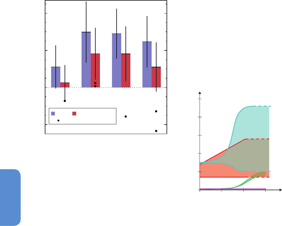
540
Chapter 6 Carbon and Other Biogeochemical Cycles
6
RCP2.6 RCP4.5 RCP6.0 RCP8.5
-200
0
200
400
Land C ssequestration, 1860-2100 (PgC)
CMIP5
explicit C-N result
CMIP5 with
inferred N constraint
Figure 6.35 | Estimated influence of nitrogen availability on total land carbon seques-
tration over the period 1860–2100 (based on analysis method of Wang and Houlton
(2009). Blue bars show, for each RCP scenario, the multi-model ensemble mean of
land carbon sequestration, based on the carbon-only subset of CMIP5 models (Cana-
dian Earth System Model 2 (CanESM2), Geophysical Fluid Dynamics Laboratory–Earth
System Model 2G (GFDL-ESM2G), Geophysical Fluid Dynamics Laboratory–Earth System
Model 2M (GFDL-ESM2M), Hadley Centre Global Environmental Model 2–Carbon
Cycle(HadGEM2-CC), Hadley Centre Global Environmental Model 2–Earth System (Had-
GEM2-ES), Institute Pierre Simon Laplace–Coupled Model 5A–Low Resolution (IPSL-
CM5A-LR), Institute Pierre Simon Laplace– Coupled Model 5A–Medium Resolution
(IPSL-CM5A-MR), Institute Pierre Simon Laplace–Coupled Model 5B–Low Resolution
(IPSL-CM5B-LR), Max Planck Institute–Earth System Model–Low Resolution (MPI-ESM-
LR): not all models produced results for all scenarios). Red bars show, for each scenario,
the mean land carbon sequestration from the same ensemble of carbon-only models
after correcting for inferred constraints on carbon uptake due to limited availability of
nitrogen. Black bars show ± one standard deviation around the means. Black symbols
show individual model results from the two CMIP5 models with explicit carbon–nitro-
gen interactions (Community Earth System Model 1–Biogeochemical (CESM1-BGC)
and Norwegian Earth System Model 1 (Emissions capable) (NorESM1-ME)). These two
models have nearly identical representations of land carbon–nitrogen dynamics, and
differences between them here (for RCP4.5 and RCP8.5, where both models contrib-
uted results) are due to differences in coupled system climate. All simulations shown
here used prescribed atmospheric CO
2
concentrations.
100
1,000
200
400
600
Timescale (yr)
Emissions
rate (TgCH
4
yr
-1
)
Anthropogenic
Wildfires
0
800
110
1000
Terrestrial permafrost
Wetlands
Figure 6.36 | Schematic synthesis of the magnitude and time scales associated with
possible future CH
4
emissions (adapted from O’Connor et al., 2010). Uncertainty in
these future changes is large, and so this figure demonstrates the relative magnitude
of possible future changes. Anthropogenic emissions starting at a present-day level of
300 Tg(CH
4
) yr
–1
(consistent with Table 6.8) and increasing or decreasing according to
RCP8.5 and RCP2.6 are shown for reference. Wetland emissions are taken as 140 to
280 Tg(CH
4
) yr
–1
present day values (Table 6.8) and increasing by between 0 and 100%
(Section 6.4.7.1; Figure 6.37). Permafrost emissions may become important during the
21st century. CH
4
release from marine hydrates and subsea permafrost may also occur
but uncertainty is sufficient to prevent plotting emission rates here. Large CH
4
hydrate
release to the atmosphere is not expected during the 21st century. No quantitative
estimates of future changes in CH
4
emissions from wildfires exist, so plotted here are
continued present-day emissions of 1 to 5 Tg(CH
4
) yr
–1
(Table 6.8).
Direct effects on wetland CH
4
emissions include: higher NPP under
higher temperature and higher atmospheric CO
2
concentrations lead-
ing to more substrate for methanogenesis (White et al., 2008); higher
CH
4
production rates under higher temperature; and changes in CH
4
oxidation through changed precipitation that alters water table posi-
tion (Melton et al., 2013). Wetland CH
4
emissions are also affected by
changes in wetland area which may either increase (due to thawing
permafrost or reduced evapotranspiration) or decrease (due to reduced
precipitation or increased evaporation) regionally. In most models, ele-
vated CO
2
has a stronger enhancement effect on CH
4
emissions than
climate change. However, large uncertainties exist concerning the lack
of wetland specific plant functional types in most models and the lack
of understanding how wetland plants will react to CO
2
fertilisation
(e.g., Berendse et al., 2001; Boardman et al., 2011; Heijmans et al.,
2001, 2002a, 2002b).
Since AR4, several modelling studies have attempted to quantify the
sensitivity of global wetland CH
4
emissions to environmental changes
(see Figure 6.37). The studies cover a wide range of simulation results
but there is high agreement between model results that the com-
bined effect of CO
2
increase and climate change by the end of the
21st century will increase wetland CH
4
emissions. Using a common
experimental protocol with spatially uniform changes in precipita-
tion, temperature and CO
2
(“WETCHIMP”; Melton et al., 2013) seven
models predict that the effect of increased temperature alone (red bars
in Figure 6.37) may cause an increase or decrease of wetland CH
4
emis-
sions, while the effect of increased precipitation alone (green bars in
Figure 6.37) is always an increase, although generally small. The effect
of increased atmospheric CO
2
concentration (fertilisation of NPP; Box
6.3; blue bars in Figure 6.37) always resulted in an increase of emis-
sions (22 to 162%). Other studies assessed the effects of temperature
and precipitation together (orange bars in Figure 6.37) and often found
an increase in wetland CH
4
emissions (Eliseev et al., 2008; Gedney et
al., 2004; Shindell et al., 2004; Volodin, 2008) although Ringeval et al.
(2011) found a net decrease. The combined effect of climate and CO
2
resulted in an increase of wetland CH
4
emissions from 40% (Volodin
(2008); fixed wetland area) to 68% (Ringeval et al., 2011); variable
wetland area).
The models assessed here do not consider changes in soil hydrologi-
cal properties caused by changes in organic matter content. Positive
feedbacks from increased drainage due to organic carbon loss may
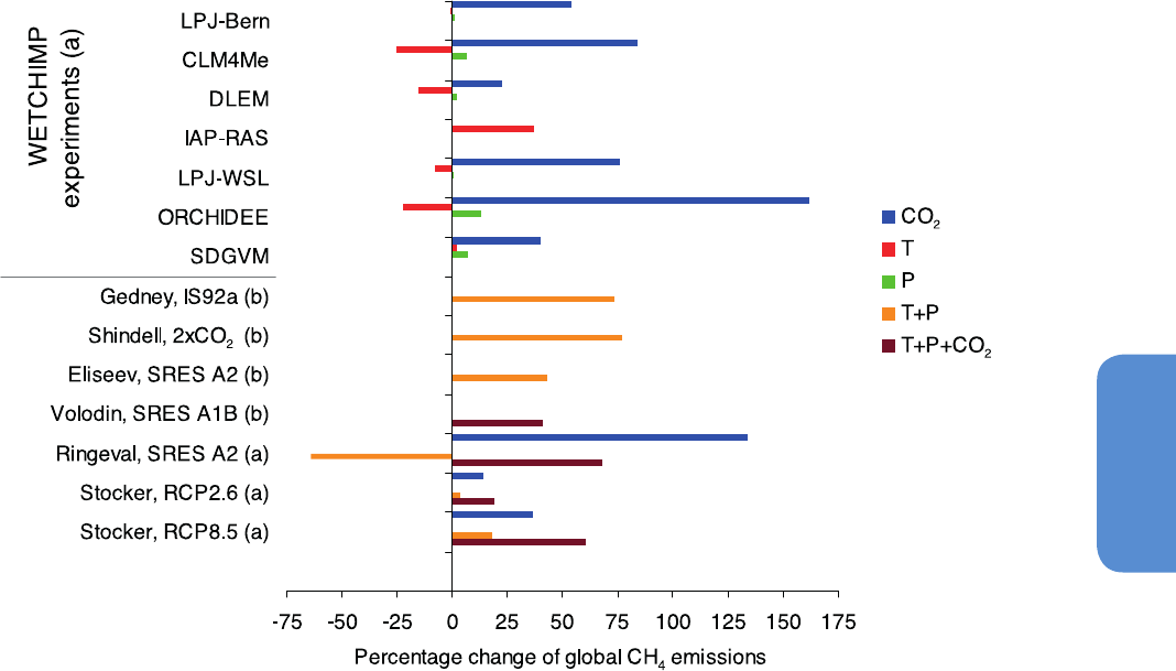
541
Carbon and Other Biogeochemical Cycles Chapter 6
6
Figure 6.37 | Relative changes of global CH
4
emissions from either pre-industrial (a) or present-day (b) conditions and environmental changes that reflect potential conditions
in 2100. The first seven models took part in the WETCHIMP intercomparison project and were run under a common protocol (Melton et al., 2013). Bars represent CH
4
emission
changes associated with temperature-only changes (T), precipitation only (P), CO
2
only (CO
2
) or combinations of multiple factors. Other studies as listed in the figure used different
future scenarios: Eliseev et al. (2008), Gedney et al. (2004), Ringeval et al. (2011), Shindell et al. (2004), Volodin (2008), Stocker et al. (2013).
accelerate peat decomposition rates (Ise et al., 2008). However, carbon
accumulation due to elevated NPP in wetland and permafrost regions
may to some extent offset CH
4
emissions (Frolking and Roulet, 2007;
Turetsky et al., 2007). None of the studies or models assessed here
considers CH
4
emissions from mangroves.
The models also do not agree in their simulations of present day wet-
land extent or CH
4
emissions, and there are not adequate data sets to
evaluate them thoroughly at the grid scale (typically 0.5°) (Melton et
al., 2013). Hence despite high agreement between models of a strong
positive response of wetland CH
4
emission rates to increasing atmo-
spheric CO
2
we assign low confidence to quantitative projections of
future wetland CH
4
emissions.
Soil CH
4
oxidation of about 30 Tg(CH
4
) yr
–1
(Table 6.8) represents the
smallest of the three sinks for atmospheric methane (see Table 6.8) but
is also sensitive to future environmental changes. Soil CH
4
oxidation is
projected to increase by up to 23% under the SRES A1B due to rising
atmospheric CH
4
concentrations, higher soil temperature and lower soil
moisture (Curry, 2007, 2009).
6.4.7.2 Future Methane Emissions from Permafrost Areas
Permafrost thaw may lead to increased drainage and a net reduction
in lakes and wetlands, a process that has already begun to be seen in
lakes in the discontinuous permafrost zone (Smith et al., 2005; Jones
et al., 2011) and has been projected to continue under future scenarios
(Avis et al., 2011). Alternatively, small lakes or ponds and wetland
growth may occur in continuous permafrost areas underlain by ice-rich
material subject to thermokarst (Christensen et al., 2004; Jorgenson et
al., 2006; Plug and West, 2009; Jones et al., 2011).
There is high agreement between land surface models that permafrost
extent is expected to reduce during the 21st century, accompanying
particularly rapid warming at high latitudes (Chapter 12). However,
estimates vary widely as to the pace of degradation (Lawrence and
Slater, 2005; Burn and Nelson, 2006; Lawrence et al., 2008). The LPJ-
WHyMe model projected permafrost area loss of 30% (SRES B1) and
47% (SRES A2) by 2100 (Wania, 2007). Marchenko et al. (2008) calcu-
late that by 2100, 57% of Alaska will lose permafrost within the top
2 m. For the RCP scenarios, the CMIP5 multi-model ensemble shows a
wide range of projections for permafrost loss: 15 to 87% under RCP4.5
and 30 to 99% under RCP8.5 (Koven et al., 2013).
Hydrological changes may lead to tradeoffs between the CO
2
and CH
4
balance of ecosystems underlain by permafrost, with methane produc-
tion rates being roughly an order of magnitude less than rates of oxic
decomposition to CO
2
but CH
4
having a larger greenhouse warming
potential (Frolking and Roulet, 2007). The extent of permafrost thaw
simulated by climate models has been used to estimate possible sub-
sequent carbon release (Burke et al., 2013; Harden et al., 2012; Section
6.4.3.4) but few studies explicitly partition this into CO
2
or CH
4
release

542
Chapter 6 Carbon and Other Biogeochemical Cycles
6
to the atmosphere. Schneider von Deimling et al. (2012) estimate cumu-
lative CH
4
emissions by 2100 between 131 and 533 Tg(CH
4
) across
the 4 RCPs. CMIP5 projections of permafrost thaw do not consider
changes in pond or lake formation. Thawing of unsaturated Yedoma
carbon deposits (which contain large, but uncertain amounts of organ-
ic carbon in permafrost in northeast Siberia; Schirrmeister et al., 2011)
was postulated to produce significant CH
4
emissions (Khvorostyanov et
al., 2008), however more recent estimates with Yedoma carbon lability
constrained by incubation observations (Dutta et al., 2006) argue for
smaller emissions at 2100 (Koven et al., 2011).
6.4.7.3 Future Methane Hydrate Emissions
Substantial quantities of methane are believed to be stored within sub-
marine hydrate deposits at continental margins (see also Section 6.1,
FAQ 6.1). There is concern that warming of overlying waters may melt
these deposits, releasing CH
4
into the ocean and atmosphere systems.
Overall, it is likely that subsequent emissions to the atmosphere caused
by hydrate destabilisation would be in the form of CO
2
, due to CH
4
oxidation in the water column.
Considering a potential warming of bottom waters by 1°C, 3°C and
5°C during the next 100 years, Reagan and Moridis (2007) found
that hydrates residing in a typical deep ocean setting (4°C and 1000
m depth) would be stable and in shallow low-latitude settings (6°C
and 560 m) any sea floor CH
4
fluxes would be oxidized within the
sediments. Only in cold-shallow Arctic settings (0.4°C and 320 m)
would CH
4
fluxes exceed rates of benthic sediment oxidation. Simula-
tions of heat penetration through the sediment by Fyke and Weaver
(2006) suggest that changes in the gas hydrate stability zone will be
small on century time scales except in high-latitude regions of shal-
low ocean shelves. In the longer term, Archer et al. (2009a) estimated
that between 35 and 940 PgC could be released over several thousand
years in the future following a 3°C seafloor warming.
Using multiple climate models (Lamarque, 2008), predicted an upper
estimate of the global sea floor flux of between 560 and 2140 Tg(CH
4
)
yr
–1
, mostly in the high latitudes. Hunter et al. (2013) also found 21st
century hydrate dissociation in shallow Arctic waters and comparable
in magnitude to Biastoch et al. (2011), although maximum CH
4
sea
floor fluxes were smaller than Lamarque (2008), with emissions from
330 to 450 Tg(CH
4
) yr
–1
for RCP 4.5 to RCP8.5. Most of the sea floor flux
of CH
4
is expected to be oxidised in the water column into dissolved
CO
2
. Mau et al. (2007) suggest only 1% might be released to the atmo-
sphere but this fraction depends on the depth of water and ocean con-
ditions. Elliott et al. (2011) demonstrated significant impacts of such
sea floor release on marine hypoxia and acidity, although atmospheric
CH
4
release was small.
Observations of CH
4
release along the Svalbard margin seafloor (West-
brook et al., 2009) suggest observed regional warming of 1°C during
the last 30 years is driving hydrate disassociation, an idea supported by
modelling (Reagan and Moridis, 2009). However, these studies do not
consider subsea-permafrost hydrates suggested recently to be region-
ally significant sources of atmospheric CH
4
(Shakhova et al., 2010).
There was no positive excursion in the methane concentration recorded
in ice cores from the largest known submarine landslide, the Storegga
slide of Norway 8200 years ago. Large methane hydrate release due to
marine landslides is unlikely as any given landslide could release only
a tiny fraction of the global inventory (Archer, 2007).
There is low confidence in modelling abilities to simulate transient
changes in hydrate inventories, but large CH
4
release to the atmo-
sphere during this century is unlikely.
6.4.8 Other Drivers of Future Carbon Cycle Changes
6.4.8.1 Changes in Fire under Climate Change/Scenarios of
Anthropogenic Fire Changes
Regional studies for boreal regions suggest an increase in future fire
risk (e.g., Amiro et al., 2009; Balshi et al., 2009; Flannigan et al., 2009a;
Spracklen et al., 2009; Tymstra et al., 2007; Westerling et al., 2011;
Wotton et al., 2010) with implications for carbon and nutrient storage
(Certini, 2005). Kurz et al. (2008b) and Metsaranta et al. (2010) indi-
cated that increased fire activity has the potential to turn the Canadi-
an forest from a sink to a source of atmospheric CO
2
. Models predict
spatially variable responses in fire activity, including strong increases
and decreases, due to regional variations in the climate–fire relation-
ship, and anthropogenic interference (Scholze et al., 2006; Flannigan et
al., 2009b; Krawchuk et al., 2009; Pechony and Shindell, 2010; Kloster
et al., 2012). Wetter conditions can reduce fire activity, but increased
biomass availability can increase fire emissions (Scholze et al., 2006;
Terrier et al., 2013). Using a land surface model and future climate
projections from two GCMs, Kloster et al. (2012) projected fire carbon
emissions in 2075–2099 that exceed present-day emissions by 17 to
62% (0.3 to 1.0 PgC yr
–1
) depending on scenario.
Future fire activity will also depend on anthropogenic factors espe-
cially related to land use change. For the Amazon it is estimated that
at present 58% of the area is too humid to allow deforestation fires
but climate change might reduce this area to 37% by 2050 (Le Page
et al., 2010). Golding and Betts (2008) estimated that future Amazon
forest vulnerability to fire may depend nonlinearly on combined cli-
mate change and deforestation.
6.4.8.2 Other Biogeochemical Cycles and Processes
Impacting Future Carbon Fluxes
6.4.8.2.1 Phosphorus
On centennial time scales, the phosphoros (P) limitation of terrestrial
carbon uptake could become more severe than the nitrogen limitation
because of limited phosphorus sources. Model simulations have shown
a shift after 2100 from nitrogen to phosphorus limitation at high lati-
tudes (Goll et al., 2012).
6.4.8.2.2 Elevated surface ozone
Plants are known to suffer damage due to exposure to levels of ozone
(O
3
) above about 40 ppb (Ashmore, 2005). Model simulations of plant
O
3
damage on the carbon cycle have found a reduction in terrestrial
carbon storage between 2005 and 2100 ranging from 4 to 140 PgC
(Felzer et al., 2005) and up to 260 PgC (Sitch et al., 2007).
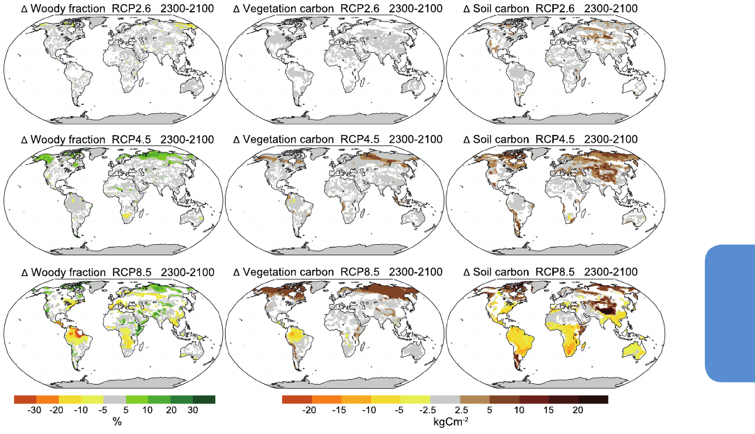
543
Carbon and Other Biogeochemical Cycles Chapter 6
6
6.4.8.2.3 Iron deposition to oceans
Changes in iron deposition may have affected ocean carbon uptake
in the past (Section 6.2.1.1), but future projections of iron deposition
from desert dust over the ocean are uncertain, even about the sign of
changes (Tegen et al., 2004; Mahowald et al., 2009). Tagliabue et al.
(2008) found relatively little impact of varying aeolian iron input on
ocean CO
2
fluxes, but Mahowald et al. (2011) show projected changes
in ocean productivity as large as those due to CO
2
increases and cli-
mate change.
6.4.8.2.4 Changes in the diffuse fraction of solar radiation
at the surface
Mercado et al. (2009) estimated that variations in the diffuse frac-
tion, associated largely with the ‘global dimming’ period (Stanhill and
Cohen, 2001), enhanced the land carbon sink by approximately 25%
between 1960 and 1999. Under heavily polluted or dark cloudy skies,
plant productivity may decline as the diffuse effect is insufficient to
offset decreased surface irradiance (UNEP, 2011). Under future scenar-
ios involving reductions in aerosol emissions (Figures 6.33 and 6.34),
the diffuse-radiation enhancement of carbon uptake will decline.
6.4.9 The Long-term Carbon Cycle and Commitments
With very high confidence, the physical, biogeochemical carbon cycle in
the ocean and on land will continue to respond to climate change and
rising atmospheric CO
2
concentrations created during the 21st century.
Long-term changes in vegetation structure and induced carbon storage
potentially show larger changes beyond 2100 than during the 21st
century as the long time scale response of tree growth and ecosystem
migrations means that by 2100 only a part of the eventual commit-
ted change will be realized (Jones et al., 2009). Holocene changes in
tree-line lagged changes in climate by centuries (MacDonald et al.,
2008). Long-term ‘commitments’ to ecosystems migration also carry
long-term committed effects to changes in terrestrial carbon storage
(Jones et al., 2010; Liddicoat et al., 2013) and permafrost (O’Connor et
al., 2010; Sections 6.4.3.3 and 6.4.7).
Warming of high latitudes is common to most climate models (Chapter
12) and this may enable increased productivity and northward expan-
sion of boreal forest ecosystems into present tundra regions depending
on nutrient availability (Kellomäki et al., 2008; Kurz et al., 2008a; Mac-
Donald et al., 2008). CMIP5 simulations by two ESMs with dynamic
vegetation for extended RCP scenarios to 2300 (Meinshausen et al.,
2011) allow analysis of this longer term response of the carbon cycle.
Increases in tree cover and terrestrial carbon storage north of 60°N are
shown in Figure 6.38.
Figure 6.38 | Maps of changes in woody cover fraction, %, (left) and terrestrial carbon storage, kg C m
–2
(vegetation carbon, middle; soil carbon, right) between years 2100
and 2300 averaged for two models, Hadley Centre Global Environmental Model 2-Earth System (HadGEM2-ES) and Max Planck Institute–Earth System Model (MPI-ESM), which
simulate vegetation dynamics for three RCP extension scenarios 2.6 (top), 4.5 (middle), and 8.5 (bottom). Note the RCP6.0 extension was not a CMIP5 required simulation. Model
results were interpolated on 1° × 1° grid; white colour indicates areas where models disagree in sign of changes. Anthropogenic land use in these extension scenarios is kept
constant at 2100 levels, so these results show the response of natural ecosystems to the climate change.
( )
( )

544
Chapter 6 Carbon and Other Biogeochemical Cycles
6
Frequently Asked Questions
FAQ 6.2 | What Happens to Carbon Dioxide After It Is Emitted into the Atmosphere?
Carbon dioxide (CO
2
), after it is emitted into the atmosphere, is firstly rapidly distributed between atmosphere, the
upper ocean and vegetation. Subsequently, the carbon continues to be moved between the different reservoirs
of the global carbon cycle, such as soils, the deeper ocean and rocks. Some of these exchanges occur very slowly.
Depending on the amount of CO
2
released, between 15% and 40% will remain in the atmosphere for up to 2000
years, after which a new balance is established between the atmosphere, the land biosphere and the ocean. Geo-
logical processes will take anywhere from tens to hundreds of thousands of years—perhaps longer—to redistribute
the carbon further among the geological reservoirs. Higher atmospheric CO
2
concentrations, and associated climate
impacts of present emissions, will, therefore, persist for a very long time into the future.
CO
2
is a largely non-reactive gas, which is rapidly mixed throughout the entire troposphere in less than a year.
Unlike reactive chemical compounds in the atmosphere that are removed and broken down by sink processes, such
as methane, carbon is instead redistributed among the different reservoirs of the global carbon cycle and ultimately
recycled back to the atmosphere on a multitude of time scales. FAQ 6.2, Figure 1 shows a simplified diagram of the
global carbon cycle. The open arrows indicate typical timeframes for carbon atoms to be transferred through the
different reservoirs.
Before the Industrial Era, the global carbon cycle was
roughly balanced. This can be inferred from ice core
measurements, which show a near constant atmo-
spheric concentration of CO
2
over the last several
thousand years prior to the Industrial Era. Anthro-
pogenic emissions of carbon dioxide into the atmo-
sphere, however, have disturbed that equilibrium. As
global CO
2
concentrations rise, the exchange process-
es between CO
2
and the surface ocean and vegetation
are altered, as are subsequent exchanges within and
among the carbon reservoirs on land, in the ocean
and eventually, the Earth crust. In this way, the added
carbon is redistributed by the global carbon cycle,
until the exchanges of carbon between the different
carbon reservoirs have reached a new, approximate
balance.
Over the ocean, CO
2
molecules pass through the
air-sea interface by gas exchange. In seawater, CO
2
interacts with water molecules to form carbonic acid,
which reacts very quickly with the large reservoir of
dissolved inorganic carbon—bicarbonate and carbon-
ate ions—in the ocean. Currents and the formation of
sinking dense waters transport the carbon between the surface and deeper layers of the ocean. The marine biota
also redistribute carbon: marine organisms grow organic tissue and calcareous shells in surface waters, which, after
their death, sink to deeper waters, where they are returned to the dissolved inorganic carbon reservoir by dissolu-
tion and microbial decomposition. A small fraction reaches the sea floor, and is incorporated into the sediments.
The extra carbon from anthropogenic emissions has the effect of increasing the atmospheric partial pressure of CO
2
,
which in turn increases the air-to-sea exchange of CO
2
molecules. In the surface ocean, the carbonate chemistry
quickly accommodates that extra CO
2
. As a result, shallow surface ocean waters reach balance with the atmosphere
within 1 or 2 years. Movement of the carbon from the surface into the middle depths and deeper waters takes
longer—between decades and many centuries. On still longer time scales, acidification by the invading CO
2
dis-
solves carbonate sediments on the sea floor, which further enhances ocean uptake. However, current understand-
ing suggests that, unless substantial ocean circulation changes occur, plankton growth remains roughly unchanged
because it is limited mostly by environmental factors, such as nutrients and light, and not by the availability of
inorganic carbon it does not contribute significantly to the ocean uptake of anthropogenic CO
2
. (continued on next page)
FAQ 6.2, Figure 1 | Simplified schematic of the global carbon cycle showing
the typical turnover time scales for carbon transfers through the major reservoirs.
VolcanismAtmosphere
Fossil fuel
emissions
>10,000 yrs
Soils
Sediments
Fossil fuel
reserves
Rocks
Earth crust
Gas exchange
from 1-10 yrs
Deep sea
from
100-2000 yrs
Surface ocean
from 10-500 yrs
from 1-100 yrs
Vegetation
Respiration
Photosynthesis
Weathering
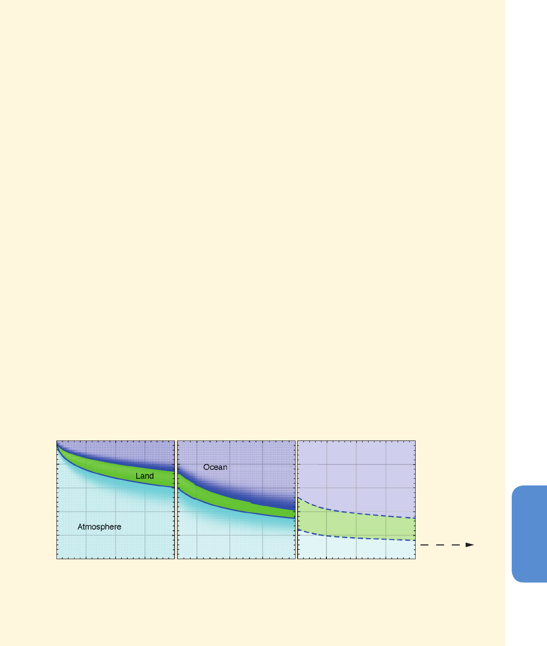
545
Carbon and Other Biogeochemical Cycles Chapter 6
6
On land, vegetation absorbs CO
2
by photosynthesis and converts it into organic matter. A fraction of this carbon is
immediately returned to the atmosphere as CO
2
by plant respiration. Plants use the remainder for growth. Dead
plant material is incorporated into soils, eventually to be decomposed by microorganisms and then respired back
into the atmosphere as CO
2
. In addition, carbon in vegetation and soils is also converted back into CO
2
by fires,
insects, herbivores, as well as by harvest of plants and subsequent consumption by livestock or humans. Some
organic carbon is furthermore carried into the ocean by streams and rivers.
An increase in atmospheric CO
2
stimulates photosynthesis, and thus carbon uptake. In addition, elevated CO
2
con-
centrations help plants in dry areas to use ground water more efficiently. This in turn increases the biomass in veg-
etation and soils and so fosters a carbon sink on land. The magnitude of this sink, however, also depends critically
on other factors, such as water and nutrient availability.
Coupled carbon-cycle climate models indicate that less carbon is taken up by the ocean and land as the climate
warms constituting a positive climate feedback. Many different factors contribute to this effect: warmer seawater,
for instance, has a lower CO
2
solubility, so altered chemical carbon reactions result in less oceanic uptake of excess
atmospheric CO
2
. On land, higher temperatures foster longer seasonal growth periods in temperate and higher
latitudes, but also faster respiration of soil carbon.
The time it takes to reach a new carbon distribution balance depends on the transfer times of carbon through the
different reservoirs, and takes place over a multitude of time scales. Carbon is first exchanged among the ‘fast’
carbon reservoirs, such as the atmosphere, surface ocean, land vegetation and soils, over time scales up to a few
thousand years. Over longer time scales, very slow secondary geological processes—dissolution of carbonate sedi-
ments and sediment burial into the Earth’s crust—become important.
FAQ 6.2, Figure 2 illustrates the decay of a large excess amount of CO
2
(5000 PgC, or about 10 times the cumulative
CO
2
emitted so far since the beginning of the industrial Era) emitted into the atmosphere, and how it is redistrib-
uted among land and the ocean over time. During the first 200 years, the ocean and land take up similar amounts
of carbon. On longer time scales, the ocean uptake dominates mainly because of its larger reservoir size (~38,000
PgC) as compared to land (~4000 PgC) and atmosphere (589 PgC prior to the Industrial Era). Because of ocean
chemistry the size of the initial input is important: higher emissions imply that a larger fraction of CO
2
will remain
in the atmosphere. After 2000 years, the atmosphere will still contain between 15% and 40% of those initial CO
2
emissions. A further reduction by carbonate sediment dissolution, and reactions with igneous rocks, such as silicate
weathering and sediment burial, will take anything from tens to hundreds of thousands of years, or even longer.
FAQ 6.2, Figure 2 | Decay of a CO
2
excess amount of 5000 PgC emitted at time zero into the atmosphere, and its subsequent redistribution into land and ocean
as a function of time, computed by coupled carbon-cycle climate models. The sizes of the colour bands indicate the carbon uptake by the respective reservoir. The first
two panels show the multi-model mean from a model intercomparison project (Joos et al., 2013). The last panel shows the longer term redistribution including ocean
dissolution of carbonaceous sediments as computed with an Earth System Model of Intermediate Complexity (after Archer et al., 2009b).
5000
4000
3000
2000
1000
0
050 100 150 200 500 10001500200040006000800010 000
(PgC)
Ocean invasion
Land uptake
Ocean invasion
Time (Years)
Land
Atmosphere
Ocean
Reaction with CaCO
3
Reactions with
igneous rocks
FAQ 6.2 (continued)

546
Chapter 6 Carbon and Other Biogeochemical Cycles
6
Increases in fire disturbance or insect damage may drive loss of forest
in temperate regions (Kurz et al., 2008c), but this process is poorly
represented or not accounted at all in models. Recent evidence from
models (Huntingford et al., 2013) and studies on climate variability
(Cox et al., 2013) suggests that large scale loss of tropical forest as pre-
viously projected in some models (Cox et al., 2004; Scholze et al., 2006)
is unlikely, but depends strongly on the predicted future changes in
regional temperature (Galbraith et al., 2010) and precipitation (Good
et al., 2011, 2013), although both models here simulate reduced tree
cover and carbon storage for the RCP8.5 scenario. ESMs also poorly
simulate resilience of ecosystems to climate changes and usually do
not account for possible existence of alternative ecosystem states such
as tropical forest or savannah (Hirota et al., 2011).
Regional specific changes in ecosystem composition and carbon stor-
age are uncertain but it is very likely that ecosystems will continue to
change for decades to centuries following stabilisation of GHGs and
climate change.
6.5 Potential Effects of Carbon Dioxide
Removal Methods and Solar Radiation
Management on the Carbon Cycle
6.5.1 Introduction to Carbon Dioxide Removal Methods
To slow or perhaps reverse projected increases in atmospheric CO
2
(Section 6.4), several methods have been proposed to increase the
removal of atmospheric CO
2
and enhance the storage of carbon in
land, ocean and geological reservoirs. These methods are categorized
as ‘Carbon Dioxide Removal (CDR)’ methods (see Glossary). Another
class of methods involves the intentional manipulation of planetary
solar absorption to counter climate change, and is called the ‘Solar
Radiation Management (SRM)’ (discussed in Chapter 7, Section 7.7;
see Glossary). In this section, CDR methods are discussed from the
aspect of the carbon cycle processes (Section 6.5.2) and their impacts
and side effects on carbon cycle and climate (Section 6.5.3). A brief
discussion on the indirect carbon cycle effects of SRM methods is given
in Section 6.5.4. Most of the currently proposed CDR methods are sum-
marized in Table 6.14 and some are illustrated schematically in Chapter
7 (Section 7.7; FAQ 7.3 Figure 1). Since some CDR methods might oper-
ate on large spatial scales they are also called ‘Geoengineering’ pro-
posals (Keith, 2001). Removal of CH
4
and N
2
O has also been proposed
to reduce climate change (Stolaroff et al., 2012). While the science of
geoengineering methods is assessed in this section (CDR) and Chapter
7 (SRM), the benefits and risks of SRM are planned to be assessed in
Chapter 19 of AR5 WGII report. Further, Chapter 6 of AR5 WGIII report
plans to assess the cost and socioeconomic implications of some CDR
and SRM methods for climate stabilization pathways.
Large-scale industrial methods such as carbon capture and storage
(CCS), biofuel energy production (without CCS) and reducing emis-
sions from deforestation and degradation (REDD) cannot be called
CDR methods since they reduce fossil fuel use or land use change CO
2
emissions to the atmosphere but they do not involve a net removal of
CO
2
that is already in the atmosphere. However, direct air capture of
CO
2
using industrial methods (Table 6.14; and FAQ 7.3 Figure 1) will
remove CO
2
from the atmosphere and is thus considered as a CDR
method. The distinction between CDR and mitigation (see Glossary) is
not clear and there could be some overlap between the two.
Insofar as the CDR-removed CO
2
is sequestered in a permanent res-
ervoir, CDR methods could potentially reduce direct consequences
of high CO
2
levels, including ocean acidification (see Section 6.4.4)
(Matthews et al., 2009). However, the effects of CDR methods that
propose to manipulate carbon cycle processes are slow (see Box 6.1)
and hence the consequent climate effects would be slow. The climate
system has a less than 5-years relaxation (e-folding) time scale for an
assumed instantaneous reduction in radiative forcing to preindustrial
levels (Held et al., 2010). While the climate effect of SRM could be
rapid (Shepherd et al., 2009) given this time scale, at present, there
is no known CDR method, including industrial direct air capture that
can feasibly reduce atmospheric CO
2
to pre-industrial levels within a
similar time scale. Therefore, CDR methods do not present an option for
rapidly preventing climate change when compared to SRM. It is likely
that CDR would have to be deployed at large-scale for at least one
century to be able to significantly reduce atmospheric CO
2
.
Important carbon cycle science considerations for evaluating CDR
methods include the associated carbon storage capacity, the perma-
nence of carbon storage and potential adverse side effects (Shepherd
et al., 2009). Geological reservoirs could store several thousand PgC
and the ocean may be able to store a few thousand PgC of anthropo-
genic carbon in the long-term (Metz et al., 2005; House et al., 2006;
Orr, 2009) (see Box 6.1 and Archer et al., 2009b). The terrestrial bio-
sphere may have a typical potential to store carbon equivalent to the
cumulative historical land use loss of 180 ± 80 PgC (Table 6.1; Section
6.5.2.1).
In this assessment, we use “permanence” to refer to time scales larger
than tens of thousands of years. CDR methods associated with either
permanent or non-permanent carbon sequestration (see Table 6.14)
have very different climate implications (Kirschbaum, 2003). Perma-
nent sequestration methods have the potential to reduce the radia-
tive forcing of CO
2
over time. By contrast, non-permanent sequestra-
tion methods will release back the temporarily sequestered carbon as
CO
2
to the atmosphere, after some delayed time interval (Herzog et
al., 2003). As a consequence, elevated levels of atmospheric CO
2
and
climate warming will only be delayed and not avoided by the imple-
mentation of non-permanent CDR methods (Figure 6.39). Neverthe-
less, CDR methods that could create a temporary CO
2
removal (Table
6.14) may still have value (Dornburg and Marland, 2008) by reducing
the cumulative impact of higher temperature.
Another important carbon cycle consequence of CDR methods is the
‘rebound effect’ (see Glossary). In the Industrial Era (since 1750) about
half of the CO
2
emitted into the atmosphere from fossil fuel emissions
has been taken up by land and ocean carbon reservoirs (see Section 6.3
and Table 6.1). As for current CO
2
emissions and the consequent CO
2
rise, which are currently opposed by uptake of CO
2
by natural reservoirs,
any removal of CO
2
from the atmosphere by CDR will be opposed by
release of CO
2
from natural reservoirs (Figure 6.40). It is thus virtually
certain that the removal of CO
2
by CDR will be partially offset by out-
gassing of CO
2
from the ocean and land ecosystems. Therefore, return-

547
Carbon and Other Biogeochemical Cycles Chapter 6
6
Carbon Cycle
Process to
be Modified
Intentionally
CDR Method Name
Nature of
CDR Removal
Process
Storage Location Storage Form
Some Carbon Cycle and
Climate Implications
Enhanced biological
production and
storage on land
Afforestation / reforestation
a
Improved forest management
b
Sequestration of wood in buildings
c
Biomass burial
d
No till agriculture
e
Biochar
f
Conservation agriculture
g
Fertilisation of land plants
h
Creation of wetlands
i
Biomass Energy with Carbon
Capture and Storage (BECCS)
j
Biological
a,b,h
Land (biomass, soils)
d
Land/ocean floor
e, f,g
Land (soils)
i
Land (wetland soils)
j
Ocean / geological
formations
a,b,c,d,e,f,g,h,i
Organic
j
Inorganic
a,b,c,d,e,f,g,h,i,j
Alters surface albedo
and evapotranspiration
a,b,c,e,f,g,h,i
Lack of permanence
d
Potentially permanent if buried on
the ocean floor
j
Permanent if stored in geological reservoir
Enhanced biological
production and
storage in ocean
Ocean iron fertilisation
k
Algae farming and burial
l
Blue carbon (mangrove, kelp farming)
m
Modifying ocean upwelling to bring
nutrients from deep ocean to surface
ocean
n
Biological Ocean
k,n
Inorganic
l,m
Organic
k
May lead to expanded regions with
low oxygen concentration, increased
N
2
O production, deep ocean acidi-
fication and disruptions to marine
ecosystems and regional carbon cycle
n
Disruptions to regional carbon cycle
Accelerated
weathering
Enhanced weathering over land
o
Enhanced weathering over ocean
p
Chemical
o
Soils and oceans
p
Ocean
o,p
Inorganic
o
Permanent removal; likely to change
pH of soils, rivers, and ocean
p
Permanent removal; likely
to change pH of ocean
Others
Direct-air capture with storage Chemical Ocean/geological formations Inorganic Permanent removal if stored
in geological reservoirs
Table 6.14 | Examples of CDR methods and their implications for carbon cycle and climate. The list is non-exhaustive. A ‘rebound’ effect and a thermal inertia of climate system
are associated with all CDR methods.
Notes
Superscripts in column 2 refer to the corresponding superscripts in columns 4, 5 and 6 of the same row.
ing to pre-industrial CO
2
levels would require permanently sequester-
ing an amount of carbon equal to total anthropogenic CO
2
emissions
that have been released before the time of CDR, roughly twice as much
the excess of atmospheric CO
2
above pre-industrial level (Lenton and
Vaughan, 2009; Cao and Caldeira, 2010b; Matthews, 2010).
6.5.2 Carbon Cycle Processes Involved in Carbon
Dioxide Removal Methods
The CDR methods listed in Table 6.14 rely primarily on human man-
agement of carbon cycle processes to remove CO
2
: (1) enhanced net
biological uptake and subsequent sequestration by land ecosystems,
(2) enhanced biological production in ocean and subsequent seques-
tration in the ocean and (3) accelerated chemical weathering reactions
over land and ocean. The exceptional CDR method is industrial direct
air capture of CO
2
, for example, relying on chemistry methods. CO
2
removed by CDR is expected to be stored in organic form on land and
in inorganic form in ocean and geological reservoirs (Table 6.14). This
management of the carbon cycle however has other implications on
ecosystems and biogeochemical cycles. The principle of different CDR
methods listed in Table 6.14 is described below and the characteristics
of some CDR methods are summarized in Table 6.15.
Some of the RCP scenarios used as a basis for future projections in this
Assessment Report already include some CDR methods. To achieve
the RCP2.6 CO
2
peak and decline the IMAGE integrated assessment
model simulates widespread implementation of BECCS technology to
achieve globally negative emissions after around 2080 (see Section
6.4.3). RCP4.5 also assumes some use of BECCS to stabilise CO
2
con-
centration by 2100. Therefore it should be noted that potentials for
CDR assessed in this section cannot be seen as additional potential
for CO
2
removal from the low RCPs as this is already included in those
scenarios.
6.5.2.1 Enhanced Carbon Sequestration by Land Ecosystems
The key driver of these CDR methods is net primary productivity on
land that currently produces biomass at a rate of approximately 50
to 60 PgC yr
–1
(Nemani et al., 2003). The principle of these CDR meth-
ods is to increase net primary productivity and/or store a larger frac-
tion of the biomass produced into ecosystem carbon pools with long
turnover times, for example, under the form of wood or refractory
organic matter in soils (Table 6.14). One variant is to harvest biomass
for energy production and sequester the emitted CO
2
(BECCS). BECCS
technology has not been tested at industrial scale, but is commonly
included in Integrated Assessment Models and future scenarios that
aim to achieve low CO
2
concentrations.
Estimates of the global potential for enhanced primary productivity
over land are uncertain because the potential of any specific method
will be severely constrained by competing land needs (e.g., agriculture,
biofuels, urbanization and conservation) and sociocultural consider-
ations. An order of magnitude of the upper potential of afforestation/
reforestation would be the restoration of all the carbon released by
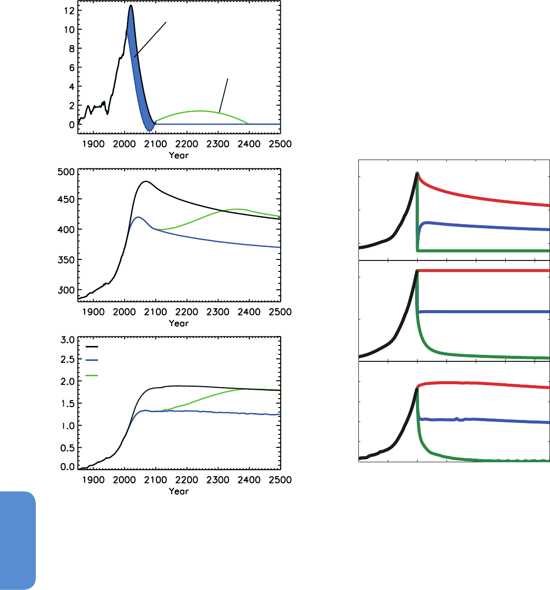
548
Chapter 6 Carbon and Other Biogeochemical Cycles
6
Figure 6.39 | Idealised model simulations (Matthews, 2010) to illustrate the effects of
CDR methods associated with either permanent or non-permanent carbon sequestra-
tion. There is an emission of 1000 PgC in the reference case (black line) between 1800
and 2100, corresponding approximately to RCP4.5 scenario (Section 6.4). Permanent
sequestration of 380 PgC, assuming no leakage of sequestered carbon would reduce cli-
mate change (blue line, compared to black line). By contrast, a non-permanent seques-
tration CDR method where carbon will be sequestered and later on returned to the
atmosphere in three centuries would not. In this idealised non-permanent sequestration
example scenario, climate change would only be delayed but the eventual magnitude of
climate change will be equivalent to the no-sequestration case (green line, compared to
black). Figure adapted from Figure 5 of Matthews (2010).
CDR-removed emissions
Re-release of CDR-removed CO
2
from non-permanent reservoirs
1000 PgC emitted; no CDR
CDR & permanent storage of 380 PgC
CDR & non-permanent storage of 380 PgC
Atmospheric CO
2
(ppm)CO
2
emissions (PgC yr
-1
)
Temperature change (°C)
Figure 6.40 | Idealised simulations with a simple global carbon cycle model (Cao and
Caldeira, 2010b) to illustrate the ‘rebound effect’. Effects of an instantaneous cessa-
tion of CO
2
emissions in the year 2050 (amber line), one-time removal of the excess
of atmospheric CO
2
over pre-industrial levels (blue line) and removal of this excess of
atmospheric CO
2
followed by continued removal of all the CO
2
that degasses from the
ocean (green line) are shown. For the years 1850–2010 observed atmospheric CO
2
con-
centrations are prescribed and CO
2
emissions are calculated from CO
2
concentrations
and modeled carbon uptake. For the years 2011–2049, CO
2
emissions are prescribed
following the SRES A2 scenario. Starting from year 2050, CO
2
emission is either set to
zero or calculated from modeled CO
2
concentrations and CO
2
uptake. To a first approxi-
mation, a cessation of emissions would prevent further warming but would not lead to
significant cooling on the century time scale. A one-time removal of excess atmospheric
CO
2
would eliminate approximately only half of the warming experienced at the time
of the removal because of CO
2
that outgases from the ocean (the rebound effect).
To bring atmospheric CO
2
back to pre-industrial levels permanently, would require the
removal of all previously emitted CO
2
, that is, an amount equivalent to approximately
twice the excess atmospheric CO
2
above pre-industrial level. (Figure adapted from Cao
and Caldeira, 2010b.)
300
400
500
1850 1950 2050 2150 2250 2350 2450
0.0
0.5
1.0
1.5
2.0
Year
0
500
1000
Zero emissions
One−time removal
Sustained removal
Atmospheric CO
2
(ppm)
Implied emissions
(PgC)
∆ Temperature
(ºC)
historical land use (180 ± 80 PgC; Table 6.1; Section 6.3.2.2). House
et al. (2002) estimated that the atmospheric CO
2
concentration by
2100 would be lowered by only about 40 to 70 ppm in that scenario
(accounting for the ‘rebound’ effect).
The capacity for enhancing the soil carbon content on agricultural and
degraded lands was estimated by one study at 50 to 60% of the his-
torical soil carbon released, that is 42 to 78 PgC (Lal, 2004a). The pro-
posed agricultural practices are the adoption of conservation tillage
with cover crops and crop residue mulch, conversion of marginal lands
into restorative land uses and nutrient cycling including the use of

549
Carbon and Other Biogeochemical Cycles Chapter 6
6
Table 6.15 | Characteristics of some CDR methods from peer-reviewed literature. Note that a variety of economic, environmental, and other constraints could also limit their
implementation and net potential.
compost and manure. Recent estimates suggest a cumulative potential
of 30 to 60 PgC of additional storage over 25 to 50 years (Lal, 2004b).
Finally, biochar and biomass burial methods aim to store organic
carbon into very long turnover time ecosystem carbon pools. The
maximum sustainable technical potential of biochar cumulative
sequestration is estimated at 130 PgC over a century by one study
(Woolf et al., 2010). The residence time of carbon converted to biochar
and the additional effect of biochar on soil productivity are uncertain,
and further research is required to assess the potential of this method
(Shepherd et al., 2009).
6.5.2.2 Enhanced Carbon Sequestration in the Ocean
The principle here is to enhance the primary productivity of phyto-
plankton (biological pump; Section 6.1.1) so that a fraction of the extra
Carbon Dioxide
Removal Method
Means of
Removing
CO
2
from
Atmosphere
Carbon
Storage /
Form
Time Scale of
Carbon Storage
Physical Potential
of CO
2
Removed
in a Century
a
Reference Unintended Side Effects
Afforestation and
reforestation
Biological Land /organic Decades to centuries 40–70 PgC House et al. (2002)
Canadell and
Raupach (2008)
Alters surface energy budget, depend-
ing on location; surface warming will
be locally increased or decreased;
hydrological cycle will be changed
Bio-energy with car-
bon-capture and stor-
age (BECCS); biomass
energy with carbon
capture and storage
Biological Geological or
ocean /inorganic
Effectively perma-
nent for geologic,
centuries for ocean
125 PgC See the footnote
b
Same as above
Biochar creation and
storage in soils
Biological Land /organic Decades to centuries 130 PgC Woolf et al. (2010) Same as above
Ocean fertilisation
by adding nutrients
to surface waters
Biological Ocean /
inorganic
Centuries to millennia 15–60 PgC
280 PgC
Aumont and Bopp (2006),
Jin and Gruber (2003)
Zeebe and Archer (2005)
Cao and Caldeira (2010a)
Expanded regions with low oxygen
concentration; enhanced N
2
O
emissions; altered production of
dimethyl sulphide and non-CO
2
greenhouse gases; possible
disruptions to marine ecosystems
and regional carbon cycles
Ocean-enhanced
upwelling bringing
more nutrients to
surface waters
Biological Ocean /
inorganic
Centuries to millennia 90 PgC
1–2 PgC
Oschlies et al. (2010a);
Lenton and Vaughan
(2009), Zhou and
Flynn (2005)
Likely to cause changes to regional
ocean carbon cycle opposing CO
2
removal, e.g., compensatory
downwelling in other regions
Land-based increased
weathering
Geochemical Ocean (and
some soils) /
inorganic
Centuries to mil-
lennia for carbon-
ates, permanent for
silicate weathering
No determined limit
100 PgC
Kelemen and Matter
(2008), Schuiling and
Krijgsman (2006)
Köhler et al. (2010)
pH of soils and rivers will increase
locally, effects on terrestrial/
freshwater ecosystems
Ocean-based
increased weathering
Geochemical Ocean /
inorganic
Centuries to mil-
lennia for carbon-
ates, permanent for
silicate weathering
No determined limit Rau (2008),
Kheshgi (1995)
Increased alkalinity effects
on marine ecosystems
Direct air capture
Chemical Geological or
ocean /inorganic
Effectively perma-
nent for geologic,
centuries for ocean
No determined limit Keith et al. (2006),
Shaffer (2010)
Not known
organic carbon produced gets transported to the deep ocean. Some
of the inorganic carbon in the surface ocean that is removed by the
export of net primary productivity below the surface layer will be sub-
sequently replaced by CO
2
pumped from the atmosphere, thus remov-
ing atmospheric CO
2
. Ocean primary productivity is limited by nutrients
(e.g., iron, nitrogen and phosphorus). Enhanced biological production
in ocean CDR methods (Table 6.14) is obtained by adding nutrients
that would otherwise be limiting (Martin, 1990). The expected increase
in the downward flux of carbon can be partly sequestered as Dissolved
Inorganic Carbon (DIC) after mineralization in the intermediate and
deep waters. In other ocean-based CDR methods, algae and kelp farm-
ing and burial, carbon would be stored in organic form.
The effectiveness of ocean CDR through iron addition depends on the
resulting increase of productivity and the fraction of this extra carbon
exported to deep and intermediate waters, and its fate. Small-scale
Notes:
a
Physical potential does not account for economic or environmental constraints of CDR methods; for example, the value of the physical potential for afforestation and reforestation does not
consider the conflicts with land needed for agricultural production. Potentials for BECCS and biochar are highly speculative.
b
If 2.5 tC yr
–1
per hectare can be harvested on a sustainable basis (Kraxner et al., 2003) on about 4% (~500 million hectares, about one tenth of global agricultural land area) of global land (13.4
billion hectares) for BECCS, approximately 1.25 PgC yr
–1
could be removed or about 125 PgC in this century. Future CO
2
concentration pathways, especially RCP2.6 and RCP4.5 include some
CO
2
removal by BECCS (Chapter 6 of AR5 WGIII) and hence the potentials estimated here cannot add on to existing model results (Section 6.4).

550
Chapter 6 Carbon and Other Biogeochemical Cycles
6
(~10 km
2
) experiments (Boyd et al., 2007) have shown only limited
transient effects of iron addition in removing atmospheric CO
2
. An
increased productivity was indeed observed, but this effect was moder-
ated either by other limiting elements, or by compensatory respiration
from increased zooplankton grazing. Most of the carbon produced by
primary productivity is oxidized (remineralized into DIC) in the surface
layer, so that only a small fraction is exported to the intermediate and
deep ocean (Lampitt et al., 2008) although some studies indicate little
remineralization in the surface layer (Jacquet et al., 2008). A recent
study (Smetacek et al., 2012) finds that at least half the extra carbon in
plankton biomass generated by artificial iron addition sank far below
a depth of 1000 m, and that a substantial portion is likely to have
reached the sea floor. There are some indications that sustained natu-
ral iron fertilisation may have a higher efficiency in exporting carbon
from surface to intermediate and deep ocean than short term blooms
induced by artificial addition of iron (Buesseler et al., 2004; Blain et al.,
2007; Pollard et al., 2009). Thus, there is no consensus on the efficiency
of iron fertilisation from available field experiments.
Using ocean carbon models (see Section 6.3.2.5.6), the maximum
drawdown of atmospheric CO
2
have been estimated from 15 ppm
(Zeebe and Archer, 2005) to 33 ppm (Aumont and Bopp, 2006) for an
idealised continuous (over 100 years) global ocean iron fertilisation,
which is technically unrealistic. In other idealised simulations of ocean
fertilisation in the global ocean or only in the Southern Ocean (Joos
et al., 1991; Peng and Broecker, 1991; Watson et al., 1994; Cao and
Caldeira, 2010a), atmospheric CO
2
was reduced by less than 100 ppm
for ideal conditions. Jin and Gruber (2003) obtained an atmospheric
drawdown of more than 60 ppm over 100 years from an idealised iron
fertilisation scenario over the entire Southern Ocean. The radiative
benefit from lower CO
2
could be offset by a few percent to more than
100% from an increase in N
2
O emissions (Jin and Gruber, 2003). All the
above estimates of maximum potential CO
2
removal account for the
rebound effect from oceans but not from the land (thus overestimate
the atmospheric CO
2
reduction).
One ocean CDR variant is to artificially supply more nutrients to the
surface ocean in upwelling areas (Lovelock and Rapley, 2007; Karl
and Letelier). The amount of carbon sequestered by these enhanced
upwelling methods critically depends on their location (Yool et al.,
2009). Idealised simulations suggest an atmospheric CO
2
removal at
a net rate of about 0.9 PgC yr
–1
(Oschlies et al., 2010b). This ocean-
based CDR method has not been tested in the field, unlike iron addition
experiments.
6.5.2.3 Accelerated Weathering
The removal of CO
2
by the weathering of silicate and carbonate miner-
als (Berner et al., 1983; Archer et al., 2009b) occurs on time scales from
thousands to tens of thousands of years (see Box 6.1) and at a rate
of ~ 0.3 PgC yr
–1
(Figure 6.1; Gaillardet et al., 1999; Hartmann et al.,
2009). This rate is currently much too small to offset the rate at which
fossil fuel CO
2
is being emitted (Section 6.3).
The principle of accelerated weathering CDR on land is to dissolve
artificially silicate minerals so drawdown of atmospheric CO
2
and
geochemical equilibrium restoration could proceed on a much faster
(century) time scale. For instance, large amounts of silicate minerals
such as olivine ((Mg,Fe)
2
SiO
4
) could be mined, crushed, transported to
and distributed on agricultural lands, to remove atmospheric CO
2
and
form carbonate minerals in soils and/or bicarbonate ions that would
be transported to the ocean by rivers (Schuiling and Krijgsman, 2006)l.
Alternatively, CO
2
removal by weathering reactions might be enhanced
by exposing minerals such as basalt or olivine to elevated CO
2
, with
potential CO
2
removal rates exceeding 0.25 PgC yr
–1
(Kelemen and
Matter, 2008). In the idealised case where olivine could be spread as a
fine powder over all the humid tropics, potential removal rates of up to
1 PgC yr
–1
have been estimated, despite limitations by the saturation
concentration of silicic acid (Köhler et al., 2010). For the United King-
dom, the potential from silicate resources was estimated to be more
than 100 PgC (Renforth, 2012).
Fossil fuel CO
2
released to the atmosphere leads to the addition of
anthropogenic CO
2
in the ocean (Section 6.3.2.5). This anthropogenic
CO
2
will eventually dissolve ocean floor carbonate sediments to reach
geochemical equilibrium on a 10 kyr time scale (Archer et al., 1997).
The principle of ocean based weathering CDR methods is to accelerate
this process. For instance, carbonate rocks could be crushed, reacted
with CO
2
(e.g., captured at power plants) to produce bicarbonate
ions that would be released to the ocean (Rau and Caldeira, 1999;
Caldeira and Rau, 2000; Rau, 2008). Alternatively, carbonate miner-
als could be directly released into the ocean (Kheshgi, 1995; Harvey,
2008). Strong bases, derived from silicate rocks, could also be released
to ocean (House et al., 2007) to increase alkalinity and drawdown
of atmospheric CO
2
. Carbonate minerals such as limestone could be
heated to produce lime (Ca(OH)
2
); this lime could be added to the
ocean to increase alkalinity as well (Kheshgi, 1995). While the level of
confidence is very high for the scientific understanding of weathering
chemical reactions, it is low for its effects and risks at planetary scale
(Section 6.5.3.3).
6.5.2.4 Carbon Dioxide Removal by Direct Industrial Capture
of Atmospheric Carbon Dioxide
Direct Air Capture refers to the chemical process by which a pure CO
2
stream is produced by capturing CO
2
from ambient air. The captured
CO
2
could be sequestered in geological reservoirs or the deep ocean. At
least three methods have been proposed to capture CO
2
from the atmo-
sphere: (1) adsorption on solids (Gray et al., 2008; Lackner, 2009, 2010;
Lackner et al., 2012); (2) absorption into highly alkaline solutions (Sto-
laroff et al., 2008; Mahmoudkhani and Keith, 2009) and (3) absorption
into moderate alkaline solution with a catalyst (Bao and Trachtenberg,
2006). The main limitation to direct air capture is the thermodynamic
barrier due to the low concentration of CO
2
in ambient air.
6.5.3 Impacts of Carbon Dioxide Removal Methods
on Carbon Cycle and Climate
One impact common to all CDR methods is related to the thermal iner-
tia of the climate system. Climate warming will indeed continue for at
least decades after CDR is applied. Therefore, temperature (and climate
change) will lag a CDR-induced decrease in atmospheric CO
2
(Boucher
et al., 2012). Modelling the impacts of CDR on climate change is still in
its infancy. Some of the first studies (Wu et al., 2010; Cao et al., 2011)

551
Carbon and Other Biogeochemical Cycles Chapter 6
6
showed that the global hydrological cycle could intensify in response
to a reduction in atmospheric CO
2
concentrations.
6.5.3.1 Impacts of Enhanced Land Carbon Sequestration
In the case of land-based CDR, biomass in forests is a non-permanent
ecosystem carbon pool and hence there is a risk that this carbon may
return to the atmosphere, for example, by disturbances such as fire, or
by future land use change. When considering afforestation/reforesta-
tion, it is also important to account for biophysical effects on climate
that come together with carbon sequestration because afforestation/
reforestation changes the albedo (see Glossary), evapotranspiration
and the roughness of the surface (Bonan, 2008; Bernier et al., 2011).
Modelling studies show that afforestation in seasonally snow covered
boreal and temperate regions will decrease the land surface albedo
and have a net (biophysical plus biogeochemical) warming effect,
whereas afforestation in low latitudes (Tropics) is likely to enhance
latent heat flux from evapotranspiration and have a net cooling effect
(Bonan et al., 1992; Betts, 2000; Bala et al., 2007; Montenegro et al.,
2009; Bathiany et al., 2010). Consequently, the location of land eco-
system based CDR methods needs to be considered carefully when
evaluating their effects on climate (Bala et al., 2007; Arora and Monte-
negro, 2011; Lee et al., 2011; Pongratz et al., 2011b). In addition CDR
in land ecosystems is likely to increase N
2
O emissions (Li et al., 2005).
Enhanced biomass production may also require more nutrients (fertilis-
ers) which are associated with fossil fuel CO
2
emission from industrial
fertiliser production and Nr impacts. Biochar-based CDR could reduce
N
2
O emissions but may increase CO
2
and CH
4
emissions from agricul-
tural soils (Wang et al., 2012b). Addition of biochar could also promote
a rapid loss of forest humus and soil carbon in some ecosystems during
the first decades (Wardle et al., 2008).
6.5.3.2 Impacts of Enhanced Carbon Sequestration in the Ocean
In the case of ocean-based CDR using fertilisation, adding macronu-
trients such as nitrogen and phosphate in the fertilised region could
lead to a decrease in production ‘downstream’ of the fertilised region
(Gnanadesikan et al., 2003; Gnanadesikan and Marinov, 2008; Watson
et al., 2008). Gnanadesikan et al. (2003) simulated a decline in export
production of 30 tC for every ton removed from the atmosphere. A
sustained global-ocean iron fertilisation for SRES A2 CO
2
emission sce-
nario was also found to acidify the deep ocean (pH decrease of about
0.1 to 0.2) while mitigating surface pH change by only 0.06 (Cao and
Caldeira, 2010a). Other environmental risks associated with ocean
fertilisation include expanded regions with low oxygen concentration
(Oschlies et al., 2010a), increased N
2
O emission (Jin and Gruber, 2003),
increased production of dimethylsulphide (DMS), isoprene, CO, N
2
O,
CH
4
and other non-CO
2
GHGs (Oschlies et al., 2010a) and possible dis-
ruptions to marine ecosystems (Denman, 2008).
In the case of enhanced ocean upwelling CDR methods there could be
disturbance to the regional carbon balances, since the extra-upwelling
will be balanced by extra-downwelling at another location. Along with
growth-supporting nutrients, enhanced concentrations of DIC will also
be brought to surface waters and partially offset the removal of CO
2
by increased biological pump. Further, in case artificially enhanced
upwelling would be stopped, atmospheric CO
2
concentrations could
rise rapidly because carbon removed from the atmosphere and stored
in soils in the cooler climate caused by artificial upwelling could be
rapidly released back (Oschlies et al., 2010b). The level of confidence
on the impacts of the enhanced upwelling is low.
6.5.3.3 Impact of Enhanced Weathering
In the case of weathering-based CDR, the pH and carbonate mineral
saturation of soils, rivers and ocean surface waters will increase where
CDR is implemented. Köhler et al. (2010) simulated that the pH of the
Amazon river would rise by 2.5 units if the dissolution of olivine in the
entire Amazon basin was used to remove 0.5 PgC yr
–1
from the atmo-
sphere. In the marine environment, elevated pH and increased alka-
linity could potentially counteract the effects of ocean acidification,
which is beneficial. Changes in alkalinity could also modify existing
ecosystems. There is uncertainty in our understanding of the net effect
on ocean CO
2
uptake but there will be a partial offset of the abiotic
effect by calcifying species. As for other CDR methods, the confidence
level on the carbon cycle impacts of enhanced weathering is low.
6.5.4 Impacts of Solar Radiation Management on the
Carbon Cycle
Solar radiation management (SRM) methods aim to reduce incoming
solar radiation at the surface (discussed in Section 7.7 and in AR5,
WG2, Chapter 19). Balancing reduced outgoing radiation by reduced
incoming radiation may be able to cool global mean temperature but
may lead to a less intense global hydrological cycle (Bala et al., 2008)
with regionally different climate impacts (Govindasamy et al., 2003;
Matthews and Caldeira, 2007; Robock et al., 2008; Irvine et al., 2010;
Ricke et al., 2010). Therefore, SRM will not prevent the effects of cli-
mate change on the carbon and other biogeochemical cycles.
SRM could reduce climate warming but will not interfere with the
direct biogeochemical effects of elevated CO
2
on the carbon cycle. For
example, ocean acidification caused by elevated CO
2
(Section 6.4.4)
and the CO
2
fertilisation of productivity (Box 6.3) will not be altered
by SRM (Govindasamy et al., 2002; Naik et al., 2003; Matthews and
Caldeira, 2007). Similarly, SRM will not interfere with the stomatal
response of plants to elevated CO
2
(the CO
2
-physiological effect) that
leads to a decline in evapotranspiration, causing land temperatures to
warm and runoff to increase (Gedney et al., 2006; Betts et al., 2007;
Matthews and Caldeira, 2007; Piao et al., 2007; Cao et al., 2010; Fyfe
et al., 2013).
However, due to carbon–climate feedbacks (Section 6.4), the imple-
mentation of SRM could affect the carbon cycle. For instance, carbon
uptake by land and ocean could increase in response to SRM by reduc-
ing the negative effects of climate change on carbon sinks (Matthews
and Caldeira, 2007). For instance, for the SRES A2 scenario with SRM,
a lower CO
2
concentration of 110 ppm by year 2100 relative to a
baseline case without SRM has been simulated by Matthews and Cal-
deira (2007). Land carbon sinks may be enhanced by increasing the
amount of diffuse relative to direct radiation (Mercado et al., 2009) if
SRM causes the fraction of diffuse light to increase (e.g., injection of
aerosols into the stratosphere). However, reduction of total incoming
solar radiation could decrease terrestrial CO
2
sinks as well.

552
Chapter 6 Carbon and Other Biogeochemical Cycles
6
6.5.5 Synthesis
CDR methods are intentional large scale methods to remove atmo-
spheric CO
2
either by managing the carbon cycle or by direct industrial
processes (Table 6.14). In contrast to SRM methods, CDR methods that
manage the carbon cycle are unlikely to present an option for rap-
idly preventing climate change. The maximum (idealised) potential for
atmospheric CO
2
removal by individual CDR methods is compiled in
Table 6.15. In this compilation, note that unrealistic assumptions about
the scale of deployment, such as fertilising the entire global ocean, are
used, and hence large potentials are simulated. The ‘rebound effect’
in the natural carbon cycle is likely to diminish the effectiveness of all
the CDR methods (Figure 6.40). The level of confidence on the effects
of both CDR and SRM methods on carbon and other biogeochemical
cycles is very low.
Acknowledgements
We wish to acknowledge Anna Peregon (LSCE, France) for investing
countless hours compiling and coordinating input from all of the Chap-
ter 6 Lead Authors. She was involved in the production of every aspect
of the chapter and we could not have completed our task on time
without her help. We also thank Brett Hopwood (ORNL, USA) for skilful
and artistic edits of several graphical figures representing the global
biogeochemical cycles in the Chapter 6 Introduction. We also thank
Silvana Schott (Max Planck Institute for Biogeochemistry, Germany) for
graphics artwork for several of the figures in Chapter 6.

553
Carbon and Other Biogeochemical Cycles Chapter 6
6
References
Achard, F., H. D. Eva, P. Mayaux, H.-J. Stibig, and A. Belward, 2004: Improved
estimates of net carbon emissions from land cover change in the tropics for the
1990s. Global Biogeochem. Cycles, 18, GB2008.
Adair, E. C., P. B. Reich, S. E. Hobbie, and J. M. H. Knops, 2009: Interactive effects
of time, CO
2
, N, and diversity on total belowground carbon allocation and
ecosystem carbon storage in a grassland community. Ecosystems, 12, 1037–
1052.
Adkins, J. F., K. McIntyre, and D. P. Schrag, 2002: The salinity, temperature and δ
18
O
of the glacial deep ocean. Science, 298, 1769–1773.
Ahn, J. and E. J. Brook, 2008: Atmospheric CO
2
and climate on millennial time scales
during the last glacial period. Science, 322, 83–85.
Ahn, J., et al., 2012: Atmospheric CO
2
over the last 1000 years: A high resolution
record from the West Antarctic Ice Sheet (WAIS) Divide ice core. Global
Biogeochem. Cycles, 26, GB2027.
Ainsworth, E. A. and S. P. Long, 2004: What have we learned from 15 years of
free-air CO
2
enrichment (FACE)? A meta-analytic review of the responses of
photosynthesis, canopy properties and plant production to rising CO
2
. New
Phytologist, 165, 351–372.
Ainsworth, E. A., C. R. Yendrek, S. Sitch, W. J. Collins, and L. D. Emberson, 2012: The
effects of tropospheric ozone on net primary productivity and implications for
climate change. Annu. Rev. Plant Biol., 63, 637–661.
Allan, W., H. Struthers, and D. C. Lowe, 2007: Methane carbon isotope effects
caused by atomic chlorine in the marine boundary layer: Global model results
compared with Southern Hemisphere measurements. J. Geophys. Res. Atmos.,
112, D04306.
Amiro, B. D., A. Cantin, M. D. Flannigan, and W. J. de Groot, 2009: Future emissions
from Canadian boreal forest fires. Can. J. Forest Res., 39, 383–395.
Anderson, R. F., M. Q. Fleisher, Y. Lao, and G. Winckler, 2008: Modern CaCO
3
preservation in equatorial Pacific sediments in the context of late-Pleistocene
glacial cycles. Mar. Chem., 111, 30–46.
Andreae, M. O. and P. Merlet, 2001: Emission of trace gases and aerosols from
biomass burning. Global Biogeochem. Cycles, 15, 955–966.
Andres, R. J., J. S. Gregg, L. Losey, G. Marland, and T. A. Boden, 2011: Monthly, global
emissions of carbon dioxide from fossil fuel consumption. Tellus B, 63, 309–327.
Andres, R. J., et al., 2012: A synthesis of carbon dioxide emissions from fossil-fuel
combustion. Biogeosciences, 9, 1845–1871.
Aranjuelo, I., et al., 2011: Maintenance of C sinks sustains enhanced C assimilation
during long-term exposure to elevated [CO
2
] in Mojave Desert shrubs. Oecologia,
167, 339–354.
Archer, D., 2007: Methane hydrate stability and anthropogenic climate change.
Biogeosciences, 4, 521–544.
Archer, D. and E. Maier-Reimer, 1994: Effect of deep-sea sedimentary calcite
preservation on atmospheric CO
2
concentration. Nature, 367, 260–263.
Archer, D. and V. Brovkin, 2008: The millennial atmospheric lifetime of anthropogenic
CO
2
. Clim. Change, 90, 283–297.
Archer, D., H. Kheshgi, and E. Maier-Reimer, 1997: Multiple timescales for
neutralization of fossil fuel CO
2
. Geophys. Res. Lett., 24, 405–408.
Archer, D., H. Kheshgi, and E. Maier-Reimer, 1998: Dynamics of fossil fuel CO
2
neutralization by marine CaCO
3
. Global Biogeochem. Cycles, 12, 259–276.
Archer, D., B. Buffett, and V. Brovkin, 2009a: Ocean methane hydrates as a slow
tipping point in the global carbon cycle. Proc. Natl. Acad. Sci. U.S.A., 106, 20596–
20601.
Archer, D., A. Winguth, D. Lea, and N. Mahowald, 2000: What caused the glacial/
interglacial atmospheric pCO
2
cycles? Rev. Geophys., 38, 159–189.
Archer, D., et al., 2009b: Atmospheric lifetime of fossil fuel carbon dioxide. Annu. Rev.
Earth Planet. Sci., 37, 117–134.
Archer, D. E., P. A. Martin, J. Milovich, V. Brovkin, G.-K. Plattner, and C. Ashendel,
2003: Model sensitivity in the effect of Antarctic sea ice and stratification on
atmospheric pCO
2
. Paleoceanography, 18, 1012.
Archibald, S., D. P. Roy, B. W. van Wilgen, and R. J. Scholes, 2009: What limits fire?
An examination of drivers of burnt area in Southern Africa. Global Change Biol.,
15, 613–630.
Arneth, A., et al., 2010: Terrestrial biogeochemical feedbacks in the climate system.
Nature Geosci., 3, 525–532.
Arora, V. K., and G. J. Boer, 2010: Uncertainties in the 20th century carbon budget
associated with land use change. Global Change Biol., 16, 3327–3348.
Arora, V. K., and A. Montenegro, 2011: Small temperature benefits provided by
realistic afforestation efforts. Nature Geosci., 4, 514–518.
Arora, V. K., et al., 2011: Carbon emission limits required to satisfy future
representative concentration pathways of greenhouse gases. Geophys. Res.
Lett., 38, L05805.
Arora, V. K., et al., 2013: Carbon-concentration and carbon-climate feedbacks in
CMIP5 Earth system models. J. Clim., 26, 5289-5314.
Artioli, Y., et al., 2012: The carbonate system in the North Sea: Sensitivity and model
validation. J. Mar. Syst., 102–104, 1–13.
Ashmore, M. R., 2005: Assessing the future global impacts of ozone on vegetation.
Plant Cell Environ., 28, 949–964.
Assmann, K. M., M. Bentsen, J. Segschneider, and C. Heinze, 2010: An isopycnic
ocean carbon cycle model. Geosci. Model Dev., 3, 143–167.
Aufdenkampe, A. K., et al., 2011: Rivering coupling of biogeochemical cycles
between land, oceans and atmosphere. Front. Ecol. Environ., 9, 23–60.
Aumont, O., and L. Bopp, 2006: Globalizing results from ocean in situ iron fertilization
studies. Global Biogeochem. Cycles, 20, GB2017.
Avis, C. A., A. J. Weaver, and K. J. Meissner, 2011: Reduction in areal extent of high-
latitude wetlands in response to permafrost thaw. Nature Geosci., 4, 444–448.
Ayres, R. U., W. H. Schlesinger, and R. H. Socolow, 1994: Human impacts on the
carbon and nitrogen cycles.In: Industrial Ecology and Global Change [R. H.
Socolow, C. Andrews, F. Berkhout and V. Thomas (eds.)]. Cambridge University
Press, Cambridge, United Kingdom, and New York, NY, USA, pp. 121–155.
Bacastow, R. B., and C. D. Keeling, 1979: Models to predict future atmospheric CO
2
concentrations. In: Workshop on the Global Effects of Carbon Dioxide from Fossil
Fuels. United States Department of Energy, Washington, DC, pp. 72–90.
Baccini, A., et al., 2012: Estimated carbon dioxide emissions from tropical
deforestation improved by carbon-density maps. Nature Clim. Change, 2, 182–
185.
Bader, M., E. Hiltbrunner, and C. Körner, 2009: Fine root responses of mature
deciduous forest trees to free air carbon dioxide enrichment (FACE). Funct. Ecol.,
23, 913–921.
Baker, A., S. Cumberland, and N. Hudson, 2008: Dissolved and total organic and
inorganic carbon in some British rivers. Area, 40, 117–127.
Baker, D. F., et al., 2006: TransCom 3 inversion intercomparison: Impact of transport
model errors on the interannual variability of regional CO
2
fluxes, 1988–2003.
Global Biogeochem. Cycles, 20, GB1002.
Bala, G., P. B. Duffy, and K. E. Taylor, 2008: Impact of geoengineering schemes on the
global hydrological cycle. Proc. Natl. Acad. Sci. U.S.A., 105, 7664–7669.
Bala, G., K. Caldeira, M. Wickett, T. J. Phillips, D. B. Lobell, C. Delire, and A. Mirin, 2007:
Combined climate and carbon-cycle effects of large-scale deforestation. Proc.
Natl. Acad. Sci. U.S.A., 104, 6550–6555.
Baldocchi, D. D., et al., 2001: FLUXNET: A new tool to study the temporal and spatial
variability of ecosystem-scale carbon dioxide, water vapor and energy flux
densities. Bull. Am. Meteorol. Soc., 82, 2415–2435.
Ballantyne, A. P., C. B. Alden, J. B. Miller, P. P. Tans, and J. W. C. White, 2012: Increase
in observed net carbon dioxide uptake by land and oceans during the last 50
years. Nature, 488, 70–72.
Balshi, M. S., A. D. McGuire, P. Duffy, M. D. Flannigan, D. W. Kicklighter, and J. Melillo,
2009: Vulnerability of carbon storage in North American boreal forests to
wildfires during the 21st century. Global Change Biol., 15, 1491–1510.
Bao, L. H., and M. C. Trachtenberg, 2006: Facilitated transport of CO
2
across a liquid
membrane: Comparing enzyme, amine, and alkaline. J. Membr. Sci., 280, 330–
334.
Barnard, R., P. W. Leadley, and B. A. Hungate, 2005: Global change, nitrification, and
denitrification: A review. Global Biogeochem. Cycles, 19, GB1007.
Barnes, R. T., and P. A. Raymond, 2009: The contribution of agricultural and urban
activities to inorganic carbon fluxes within temperate watersheds. Chem. Geol.,
266, 318–327.
Barnosky, A. D., 2008: Colloquium Paper: Megafauna biomass tradeoff as a driver
of Quaternary and future extinctions. Proc. Natl. Acad. Sci. U.S.A., 105, 11543–
11548.
Bastviken, D., J. Cole, M. Pace, and L. Tranvik, 2004: Methane emissions from lakes:
Dependence of lake characteristics, two regional assessments, and a global
estimate. Global Biogeochem. Cycles, 18, GB4009.

554
Chapter 6 Carbon and Other Biogeochemical Cycles
6
Bastviken, D., L. J. Tranvik, J. A. Downing, P. M. Crill, and A. Enrich-Prast, 2011:
Freshwater methane emissions offset the continental carbon sink. Science, 331,
50.
Bathiany, S., M. Claussen, V. Brovkin, T. Raddatz, and V. Gayler, 2010: Combined
biogeophysical and biogeochemical effects of large-scale forest cover changes
in the MPI earth system model. Biogeosciences, 7, 1383–1399.
Batjes, N. H., 1996: Total carbon and nitrogen in the soils of the world. Eur. J. Soil
Sci., 47, 151–163.
Battin, T. J., S. Luyssaert, L. A. Kaplan, A. K. Aufdenkampe, A. Richter, and L. J. Tranvik,
2009: The boundless carbon cycle Nature Geosci., 2, 598–600.
Beaugrand, G., M. Edwards, and L. Legendre, 2010: Marine biodiversity, ecosystem
functioning, and carbon cycles. Proc. Natl. Acad. Sci. U.S.A., 107, 10120–10124.
Beaulieu, J. J., et al., 2011: Nitrous oxide emission from denitrification in stream and
river networks. Proc. Natl. Acad. Sci. U.S.A., 108, 214–219.
Beer, C., et al., 2010: Terrestrial gross carbon dioxide uptake: Global distribution and
covariation with climate. Science, 329, 834-838.
Bellassen, V., G. Le Maire, J. F. Dhote, P. Ciais, and N. Viovy, 2010: Modelling forest
management within a global vegetation model. Part 1: Model structure and
general behaviour. Ecol. Model., 221, 2458–2474.
Bellassen, V., N. Viovy, S. Luyssaert, G. Le Maire, M.-J. Schelhaas, and P. Ciais, 2011:
Reconstruction and attribution of the carbon sink of European forests between
1950 and 2000. Global Change Biol., 17, 3274–3292.
Bennington, V., G. A. McKinley, S. Dutkiewicz, and D. Ullman, 2009: What does
chlorophyll variability tell us about export and air-sea CO
2
flux variability in the
North Atlantic? Global Biogeochem. Cycles, 23, GB3002.
Berendse, F., et al., 2001: Raised atmospheric CO
2
levels and increased N deposition
cause shifts in plant species composition and production in Sphagnum bogs.
Global Change Biol., 7, 591–598.
Bergamaschi, P., et al., 2009: Inverse modeling of global and regional CH
4
emissions
using SCIAMACHY satellite retrievals. J. Geophys. Res., 114, D22301.
Berger, W. H., 1982: Increase of carbon dioxide in the atmosphere during deglaciation:
The coral-reef hypothesis. Naturwissenschaften, 69, 87–88.
Berner, R. A., 1992: Weathering, plants, and the long-term carbon-cycle. Geochim.
Cosmochim. Acta, 56, 3225–3231.
Berner, R. A., A. C. Lasaga, and R. M. Garrels, 1983: The carbonate-silicate
geochemical cycle and its effect on atmospheric carbon dioxide over the past
100 million years. Am. J. Sci., 283, 641–683.
Bernier, P. Y., R. L. Desjardins, Y. Karimi-Zindashty, D. E. Worth, A. Beaudoin, Y. Luo,
and S. Wang, 2011: Boreal lichen woodlands: A possible negative feedback to
climate change in Eastern North America. Agr. Forest Meteorol., 151, 521–528.
Betts, R. A., 2000: Offset of the potential carbon sink from boreal forestation by
decreases in surface albedo. Nature, 408, 187–190.
Betts, R. A., et al., 2007: Projected increase in continental runoff due to plant
responses to increasing carbon dioxide. Nature, 448, 1037–1041.
Bianchi, D., J. P. Dunne, J. L. Sarmiento, and E. D. Galbraith, 2012: Data-based
estimates of suboxia, denitrification and N
2
O production in the ocean and their
sensitivity to dissolved O
2
. Global Biogeochem. Cycles, 26, GB2009.
Biastoch, A., et al., 2011: Rising Arctic Ocean temperatures cause gas hydrate
destabilization and ocean acidification. Geophys. Res. Lett., 38, L08602.
Billings, S. A., S. M. Schaeffer, and R. D. Evans, 2002: Trace N gas losses and N
mineralization in Mojave desert soils exposed to elevated CO
2
. Soil Biol.
Biochem., 34, 1777–1784.
Bird, M. I., J. Lloyd, and G. D. Farquhar, 1996: Terrestrial carbon storage from the last
glacial maximum to the present. Chemosphere, 33, 1675–1685.
Blain, S., et al., 2007: Effect of natural iron fertilization on carbon sequestration in
the Southern Ocean. Nature, 446, 1070–1074.
Blake, D. R., E. W. Mayer, S. C. Tyler, Y. Makide, D. C. Montague, and F. S. Rowland,
1982: Global increase in atmospheric methane concentrations between 1978
and 1980. Geophys. Res. Lett., 9, 477–480.
Bleeker, A., W. K. Hicks, F. Dentener, and J. Galloway, 2011: Nitrogen deposition as
a threat to the World’s protected areas under the Convention on Biological
Diversity. Environ. Pollut., 159, 2280–2288.
Bloom, A. A., J. Lee-Taylor, S. Madronich, D. J. Messenger, P. I. Palmer, D. S. Reay,
and A. R. McLeod, 2010: Global methane emission estimates from ultraviolet
irradiation of terrestrial plant foliage. New Phytologist, 187, 417–425.
Blunier, T., J. Chappellaz, J. Schwander, B. Stauffer, and D. Raynaud, 1995: Variations
in atmospheric methane concentration during the Holocene epoch. Nature, 374,
46–49.
Boardman, C. P., V. Gauci, J. S. Watson, S. Blake, and D. J. Beerling, 2011: Contrasting
wetland CH
4
emission responses to simulated glacial atmospheric CO
2
in
temperate bogs and fens. New Phytologist, 192, 898–911.
Bock, M., J. Schmitt, L. Moller, R. Spahni, T. Blunier, and H. Fischer, 2010: Hydrogen
isotopes preclude marine hydrate CH
4
emissions at the onset of Dansgaard-
Oeschger events. Science, 328, 1686–1689.
Boden, T., G. Marland, and R. Andres, 2011: Global CO
2
emissions from fossil-
fuel burning, cement manufacture, and gas flaring: 1751–2008 (accessed
at 2011.11.10). Oak Ridge National Laboratory, U. S. Department of Energy,
Carbon Dioxide Information Analysis Center, Oak Ridge, TN, U.S.A., doi:10.3334/
CDIAC/00001_V2011, http://cdiac.ornl.gov/trends/emis/overview_2008.html.
Bonan, G. B., 2008: Ecological Climatology: Concepts and Applications. Cambridge
University Press, New York, NY, USA.
Bonan, G. B., and S. Levis, 2010: Quantifying carbon-nitrogen feedbacks in the
Community Land Model (CLM4). Geophys. Res. Lett., 37, L07401.
Bonan, G. B., D. Pollard, and S. L. Thompson, 1992: Effects of boreal forest vegetation
on global climate. Nature, 359, 716–718.
Bond-Lamberty, B., and A. Thomson, 2010: Temperature-associated increases in the
global soil respiration record. Nature, 464, 579–U132.
Booth, B. B. B., et al., 2012: High sensitivity of future global warming to land carbon
cycle processes. Environ. Res. Lett., 7, 024002.
Bopp, L., K. E. Kohfeld, C. Le Quéré, and O. Aumont, 2003: Dust impact on marine
biota and atmospheric CO
2
during glacial periods. Paleoceanography, 18, 1046.
Bopp, L., C. Le Quéré, M. Heimann, A. C. Manning, and P. Monfray, 2002: Climate-
induced oceanic oxygen fluxes: Implications for the contemporary carbon
budget. Global Biogeochem. Cycles, 16, 1022.
Bopp, L., et al., 2001: Potential impact of climate change on marine export
production. Global Biogeochem. Cycles, 15, 81–99.
Boucher, O., et al., 2012: Reversibility in an Earth System model in response to CO
2
concentration changes. Environ. Res. Lett., 7, 024013.
Bousquet, P., D. A. Hauglustaine, P. Peylin, C. Carouge, and P. Ciais, 2005: Two
decades of OH variability as inferred by an inversion of atmospheric transport
and chemistry of methyl chloroform. Atmos. Chem. Phys., 5, 2635–2656.
Bousquet, P., P. Peylin, P. Ciais, C. Le Quéré, P. Friedlingstein, and P. P. Tans, 2000:
Regional changes in carbon dioxide fluxes of land and oceans since 1980.
Science, 290, 1342–1346.
Bousquet, P., et al., 2006: Contribution of anthropogenic and natural sources to
atmospheric methane variability. Nature, 443, 439–443.
Bousquet, P., et al., 2011: Source attribution of the changes in atmospheric methane
for 2006–2008. Atmos. Chem. Phys., 11, 3689–3700.
Bouttes, N., D. Paillard, D. M. Roche, V. Brovkin, and L. Bopp, 2011: Last Glacial
Maximum CO
2
and d
13
C successfully reconciled. Geophys. Res. Lett., 38, L02705.
Bouttes, N., et al., 2012: Impact of oceanic processes on the carbon cycle during the
last termination. Clim. Past, 8, 149–170.
Bouwman, A. F., et al., 2013: Global trends and uncertainties in terrestrial
denitrification and N
2
O emissions. Philos. Trans. R. Soc. London Ser. B, 368,
20130112.
Bouwman, L., et al., 2011: Exploring global changes in nitrogen and phosphorus
cycles in agriculture induced by livestock production over the 1900–2050
period. Proc. Natl. Acad. Sci. U.S.A., doi:10.1073/pnas.1012878108.
Boyd, P. W., et al., 2007: Mesoscale iron enrichment experiments 1993–2005:
Synthesis and future directions. Science, 315, 612–617.
Bozbiyik, A., M. Steinacher, F. Joos, T. F. Stocker, and L. Menviel, 2011: Fingerprints of
changes in the terrestrial carbon cycle in response to large reorganizations in
ocean circulation. Clim. Past, 7, 319–338.
Brenninkmeijer, C. A. M., et al., 2007: Civil Aircraft for the regular investigation of
the atmosphere based on an instrumented container: The new CARIBIC system.
Atmos. Chem. Phys., 7, 4953–4976.
Bridgham, S. D., J. P. Megonigal, J. K. Keller, N. B. Bliss, and C. Trettin, 2006: The carbon
balance of North American wetlands. Wetlands, 26, 889–916.
Broecker, W. S., and T.-H. Peng, 1986: Carbon cycle: 1985 glacial to interglacial
changes in the operation of the global carbon cycle. Radiocarbon, 28, 309–327.
Broecker, W. S., E. Clark, D. C. McCorkle, T.-H. Peng, I. Hajdas, and G. Bonani, 1999:
Evidence for a reduction in the carbonate ion content of the deep sea during the
course of the Holocene. Paleoceanography, 14, 744–752.
Brovkin, V., A. Ganopolski, D. Archer, and S. Rahmstorf, 2007: Lowering of glacial
atmospheric CO
2
in response to changes in oceanic circulation and marine
biogeochemistry. Paleoceanography, 22, PA4202.

555
Carbon and Other Biogeochemical Cycles Chapter 6
6
Brovkin, V., J. H. Kim, M. Hofmann, and R. Schneider, 2008: A lowering effect of
reconstructed Holocene changes in sea surface temperatures on the atmospheric
CO
2
concentration. Global Biogeochem. Cycles, 22, GB1016.
Brovkin, V., T. Raddatz, C. H. Reick, M. Claussen, and V. Gayler, 2009: Global
biogeophysical interactions between forest and climate. Geophys. Res. Lett., 36,
L07405.
Brovkin, V., S. Sitch, W. von Bloh, M. Claussen, E. Bauer, and W. Cramer, 2004: Role of
land cover changes for atmospheric CO
2
increase and climate change during the
last 150 years. Global Change Biol., 10, 1253–1266.
Brovkin, V., J. Bendtsen, M. Claussen, A. Ganopolski, C. Kubatzki, V. Petoukhov, and A.
Andreev, 2002: Carbon cycle, vegetation, and climate dynamics in the Holocene:
Experiments with the CLIMBER-2 model. Global Biogeochem. Cycles, 16, 1139.
Brovkin, V., et al., 2010: Sensitivity of a coupled climate-carbon cycle model to large
volcanic eruptions during the last millennium. Tellus B, 62, 674–681.
Brown, J. R., et al., 2011: Effects of multiple global change treatments on soil N
2
O
fluxes. Biogeochemistry, 109, 85–100.
Brzezinski, M. A., et al., 2002: A switch from Si(OH)
4
to NO
3
depletion in the glacial
Southern Ocean. Geophys. Res. Lett., 29, 1564.
Buesseler, K. O., J. E. Andrews, S. M. Pike, and M. A. Charette, 2004: The effects of
iron fertilization on carbon sequestration in the Southern Ocean. Science, 304,
414–417.
Burke, E. J., C. D. Jones, and C. D. Koven, 2013: Estimating the permafrost-carbon-
climate response in the CMIP5 climate models using a simplified approach. J.
Clim., 26, 4897-4909.
Burn, C. R., and F. E. Nelson, 2006: Comment on “A projection of severe near-surface
permafrost degradation during the 21st century” by David M. Lawrence and
Andrew G. Slater. Geophys. Res. Lett., 33, L21503.
Butterbach-Bahl, K., and M. Dannenmann, 2011: Denitrification and associated soil
N
2
O emissions due to agricultural activities in a changing climate. Curr. Opin.
Environ. Sustain., 3, 389–395.
Byrne, R. H., S. Mecking, R. A. Feely, and X. W. Liu, 2010: Direct observations of basin-
wide acidification of the North Pacific Ocean. Geophys. Res. Lett., 37, L02601.
Cadule, P., et al., 2010: Benchmarking coupled climate-carbon models against long-
term atmospheric CO
2
measurements. Global Biogeochem. Cycles, 24, GB2016.
Cai, W.-J., et al., 2011: Acidification of subsurface coastal waters enhanced by
eutrophication. Nature Geosci, 4, 766–770.
Caldeira, K., and G. H. Rau, 2000: Accelerating carbonate dissolution to sequester
carbon dioxide in the ocean: Geochemical implications. Geophys. Res. Lett., 27,
225–228.
Caldeira, K., and M. E. Wickett, 2005: Ocean model predictions of chemistry changes
from carbon dioxide emissions to the atmosphere and ocean. J. Geophys. Res.
Oceans, 110, C09S04.
Canadell, J. G., and M. R. Raupach, 2008: Managing forests for climate change
mitigation. Science, 320, 1456–1457.
Canadell, J. G., et al., 2007a: Saturation of the terrestrial carbon sink. In: Terrestrial
Ecosystems in a Changing World. [J. G. Canadell, D. Pataki and L. Pitelka (eds.)].
The IGBP Series. Springer-Verlag, Berlin and Heidelberg, Germany, pp. 59–78,
Canadell, J. G., et al., 2007b: Contributions to accelerating atmospheric CO
2
growth
from economic activity, carbon intensity, and efficiency of natural sinks. Proc.
Natl. Acad. Sci. U.S.A., 104, 18,866–18,870.
Canfield, D. E., A. N. Glazer, and P. G. Falkowski, 2010: The evolution and future of
Earth’s nitrogen cycle. Science, 330, 192–196.
Cao, L., and K. Caldeira, 2010a: Can ocean iron fertilization mitigate ocean
acidification? Clim. Change, 99, 303–311.
Cao, L., and K. Caldeira, 2010b: Atmospheric carbon dioxide removal: Long-term
consequences and commitment. Environ. Res. Lett., 5, 024011.
Cao, L., K. Caldeira, and A. K. Jain, 2007: Effects of carbon dioxide and climate
change on ocean acidification and carbonate mineral saturation. Geophys. Res.
Lett., 34, L05607.
Cao, L., G. Bala, and K. Caldeira, 2011: Why is there a short-term increase in global
precipitation in response to diminished CO
2
forcing? Geophys. Res. Lett., 38,
L06703.
Cao, L., G. Bala, K. Caldeira, R. Nemani, and G. Ban-Weiss, 2010: Importance of
carbon dioxide physiological forcing to future climate change. Proc. Natl. Acad.
Sci. U.S.A., 107, 9513–9518.
Carcaillet, C., et al., 2002: Holocene biomass burning and global dynamics of the
carbon cycle. Chemosphere, 49, 845–863.
Certini, G., 2005: Effects of fire on properties of forest soils: A review. Oecologia,
143, 1–10.
Chambers, J. Q., J. I. Fisher, H. Zeng, E. L. Chapman, D. B. Baker, and G. C. Hurtt, 2007:
Hurricane Katrina’s carbon footprint on U.S. Gulf Coast forests. Science, 318,
1107.
Chantarel, A. M., J. M. G. Bloor, N. Deltroy, and J.-F. Soussana, 2011: Effects of climate
change drivers on nitrous oxide fluxes in an upland temperate grassland.
Ecosystems, 14, 223–233.
Chapuis-Lardy, L., N. Wrage, A. Metay, J. L. Chotte, and M. Bernoux, 2007: Soils, a
sink for N
2
O? A review. Global Change Biol., 13, 1–17.
Chen, Y. H., and R. G. Prinn, 2006: Estimation of atmospheric methane emissions
between 1996 and 2001 using a three-dimensional global chemical transport
model. J. Geophys. Res. Atmos., 111, D10307.
Chhabra, A., K. R. Manjunath, S. Panigrahy, and J. S. Parihar, 2013: Greenhouse gas
emissions from Indian livestock. Clim. Change, 117, 329–344.
Chierici, M., and A. Fransson, 2009: Calcium carbonate saturation in the surface
water of the Arctic Ocean: Undersaturation in freshwater influenced shelves.
Biogeosciences, 6, 2421–2431.
Christensen, T. R., et al., 2004: Thawing sub-arctic permafrost: Effects on vegetation
and methane emissions. Geophys. Res. Lett., 31, L04501.
Churkina, G., V. Brovkin, W. von Bloh, K. Trusilova, M. Jung, and F. Dentener, 2009:
Synergy of rising nitrogen depositions and atmospheric CO
2
on land carbon
uptake moderately offsets global warming. Global Biogeochem. Cycles, 23,
GB4027.
Ciais, P., P. Rayner, F. Chevallier, P. Bousquet, M. Logan, P. Peylin, and M. Ramonet,
2010: Atmospheric inversions for estimating CO
2
fluxes: methods and
perspectives. Clim. Change, 103, 69–92(24).
Ciais, P., et al., 2012: Large inert carbon pool in the terrestrial biosphere during the
Last Glacial Maximum. Nature Geosci., 5, 74–79.
Ciais, P., et al., 2008: Carbon accumulation in European forests. Nature Geosci., 1,
425–429.
Ciais, P., et al., 2005: Europe-wide reduction in primary productivity caused by the
heat and drought in 2003. Nature, 437, 529–533.
Clark, D. B., D. A. Clark, and S. F. Oberbauer, 2010: Annual wood production in a
tropical rain forest in NE Costa Rica linked to climatic variation but not to
increasing CO
2
. Global Change Biol., 16, 747–759.
Claussen, M., et al., 2002: Earth system models of intermediate complexity: Closing
the gap in the spectrum of climate system models. Clim. Dyn., 18, 579–586.
Cocco, V., et al., 2013: Oxygen and indicators of stress for marine life in multi-model
global warming projections. Biogeosciences, 10, 1849–1868.
Codispoti, L. A., 2007: An oceanic fixed nitrogen sink exceeding 400 Tg N a
−1
vs
the concept of homeostasis in the fixed-nitrogen inventory. Biogeosciences, 4,
233–253.
Codispoti, L. A., 2010: Interesting Times for Marine N
2
O. Science, 327, 1339–1340.
Cole, J. J., et al., 2007: Plumbing the global carbon cycle: Integrating inland waters
into the terrestrial carbon budget. Ecosystems, 10, 171–184.
Collins, W. J., et al., 2011: Development and evaluation of an Earth-System model—
HadGEM2. Geosci. Model Dev., 4, 1051–1075.
Conrad, R., 1996: Soil microorganisms as controllers of atmospheric trace gases (H
2
,
CO, CH
4
, OCS, N
2
O, and NO). Microbiol. Rev., 60, 609–640.
Conway, T., and P. Tans, 2011: Global CO
2
. National Oceanic and Atmospheric
Administration, Earth System Research Library, Silver Spring, MD, USA.
Conway, T. J., P. P. Tans, L. S. Waterman, K. W. Thoning, D. R. Kitzis, K. A. Masarie, and
N. Zhang, 1994: Evidence for interannual variability of the carbon cycle from
the National Oceanic and Atmospheric Administration Climate Monitoring and
Diagnostics Laboratory Global Air Sampling Network. J. Geophys. Res. Atmos.,
99, 22831–22855.
Corbière, A., N. Metzl, G. Reverdin, C. Brunet, and A. Takahashi, 2007: Interannual
and decadal variability of the oceanic carbon sink in the North Atlantic subpolar
gyre. Tellus B, 59, 168–178.
Cox, P., and C. Jones, 2008: Climate change. Illuminating the modern dance of
climate and CO
2
. Science, 321, 1642–1644.
Cox, P. M., 2001: Description of the TRIFFID dynamic global vegetation model.
Technical Note 24. Hadley Centre, Met Office, Exeter, Devon, UK.
Cox, P. M., R. A. Betts, M. Collins, P. P. Harris, C. Huntingford, and C. D. Jones, 2004:
Amazonian forest dieback under climate-carbon cycle projections for the 21st
century. Theor. Appl. Climatol., 78, 137–156.
Cox, P. M., D. Pearson, B. B. Booth, P. Friedlingstein, C. Huntingford, C. D. Jones, and
C. M. Luke, 2013: Sensitivity of tropical carbon to climate change constrained by
carbon dioxide variability. Nature, 494, 341–344.

556
Chapter 6 Carbon and Other Biogeochemical Cycles
6
Crévoisier, C., D. Nobileau, A. M. Fiore, R. Armante, A. Chédin, and N. A. Scott, 2009:
Tropospheric methane in the tropics – first year from IASI hyperspectral infrared
observations. Atmos. Chem. Phys., 9, 6337–6350.
Crutzen, P. J., A. R. Mosier, K. A. Smith, and W. Winiwarter, 2008: N
2
O release from
agro-biofuel production negates global warming reduction by replacing fossil
fuels. Atmos. Chem. Phys., 8, 389–395.
Cunnold, D. M., et al., 2002: In situ measurements of atmospheric methane at GAGE/
AGAGE sites during 1985–2000 and resulting source inferences. J. Geophys. Res.
Atmos., 107, ACH20–1, CiteID 4225.
Curry, C. L., 2007: Modeling the soil consumption of methane at the global scale.
Global Biogeochem. Cycles, 21, GB4012.
Curry, C. L., 2009: The consumption of atmospheric methane by soil in a simulated
future climate. Biogeosciences, 6, 2355–2367.
Daniau, A. L., et al., 2012: Predictability of biomass burning in response to climate
changes. Global Biogeochem. Cycles, 26, Gb4007.
Davidson, E. A., 2009: The contribution of manure and fertilizer nitrogen to
atmospheric nitrous oxide since 1860. Nature Geosci., 2, 659–662.
Davidson, E. A., et al., 2012: Excess nitrogen in the U.S. environnement: Trends,
risks, and solutions. Issues of Ecology, Report number 15. Ecological Society of
America, Washington, DC.
Dawes, M. A., S. Hättenschwiler, P. Bebi, F. Hagedorn, I. T. Handa, C. Körner, and C.
Rixen, 2011: Species-specific tree growth responses to 9 years of CO
2
enrichment
at the alpine treeline. J. Ecol., 99, 383–394.
De Klein, C., et al., 2007: N
2
O emissions from managed soils, and CO
2
emissions from
lime and urea application. In: 2006 IPCC Guidelines for National Greenhouse
Gas Inventories, Vol. 4 [M. Gytarsky, T. Higarashi, W. Irving, T. Krug and J. Penman
(eds.)]. Intergovernmental Panel on Climate Change, Geneva, Switzerland, pp.
11.1–11.54.
DeFries, R., and C. Rosenzweig, 2010: Toward a whole-landscape approach for
sustainable land use in the tropics. Proc. Natl. Acad. Sci. U.S.A., 107, 19627–
19632.
DeFries, R. S., R. A. Houghton, M. C. Hansen, C. B. Field, D. L. Skole, and J. Townshend,
2002: Carbon emissions from tropical deforestation and regrowth based on
satellite observations for the 1980s and 1990s. Proc. Natl. Acad. Sci. U.S.A., 99,
14256–14261.
Delmas, R. J., J.-M. Ascencio, and M. Legrand, 1980: Polar ice evidence that
atmospheric CO
2
20,000–yr BP was 50% of present. Nature, 284, 155–157.
Denman, K. L., 2008: Climate change, ocean processes and ocean iron fertilization.
Mar. Ecol. Prog. Ser., 364, 219–225.
Denman, K. L., et al., 2007: Couplings between changes in the climate system
and biogeochemistry. In: Climate Change 2007: The Physical Science Basis.
Contribution of Working Group I to the Fourth Assessment Report of the
Intergovernmental Panel on Climate Change [Solomon, S., D. Qin, M. Manning,
Z. Chen, M. Marquis, K. B. Averyt, M. Tignor and H. L. Miller (eds.)] Cambridge
University Press, Cambridge, United Kingdom and New York, NY, USA, 499-587.
Dentener, F., W. Peters, M. Krol, M. van Weele, P. Bergamaschi, and J. Lelieveld, 2003:
Interannual variability and trend of CH
4
lifetime as a measure for OH changes in
the 1979–1993 time period. J. Geophys. Res. Atmos., 108, 4442.
Dentener, F., et al., 2005: The impact of air pollutant and methane emission controls
on tropospheric ozone and radiative forcing: CTM calculations for the period
1990–2030. Atmos. Chem. Phys., 5, 1731–1755.
Dentener, F., et al., 2006: The global atmospheric environment for the next
generation. Environ. Sci. Technol., 40, 3586–3594.
Deutsch, C., J. L. Sarmiento, D. M. Sigman, N. Gruber, and J. P. Dunne, 2007: Spatial
coupling of nitrogen inputs and losses in the ocean. Nature, 445, 163–167.
Dickens, G. R., 2003: A methane trigger for rapid warming? Science, 299, 1017.
Dlugokencky, E., and P. P. Tans, 2013a: Recent CO
2,
NOAA, ESRS. Retrieved from
www.esrl.noaa.gov/gmd/ccgg/trends/global.html, accessed 01-02-2013.
Dlugokencky, E., and P. P. Tans, 2013b: Globally averaged marine surface annual
mean data, NOAA/ESRL. Retrieved from www.esrl.noaa.gov/gmd/ccgg/trends/,
accessed 01-02-2013.
Dlugokencky, E. J., E. G. Nisbet, R. Fisher, and D. Lowry, 2011: Global atmospheric
methane: Budget, changes and dangers. Philos. Trans. R. Soc. London Ser. A, 369,
2058–2072.
Dlugokencky, E. J., P. M. Lang, A. M. Crotwell, and K. A. Masarie, 2012: Atmospheric
methane dry air mole fractions from the NOAA ESRL Carbon Cycle Cooperative
Global Air Sampling Network, 1983–2011, version 2012-09-24. Version 2010-
08-12 ed.
Dlugokencky, E. J., S. Houweling, L. Bruhwiler, K. A. Masarie, P. M. Lang, J. B. Miller,
and P. P. Tans, 2003: Atmospheric methane levels off: Temporary pause or a new
steady-state? Geophys. Res. Lett., 30, 1992.
Dlugokencky, E. J., et al., 2009: Observational constraints on recent increases in the
atmospheric CH
4
burden. Geophys. Res. Lett., 36, L18803.
Dolman, A. J., et al., 2012: An estimate of the terrestrial carbon budget of Russia
using inventory based, eddy covariance and inversion methods. Biogeosciences,
9, 5323–5340.
Doney, S. C., et al., 2009: Mechanisms governing interannual variability in upper-
ocean inorganic carbon system and air-sea CO
2
fluxes: Physical climate and
atmospheric dust. Deep-Sea Res. Pt. II, 56, 640–655.
Dore, J. E., R. Lukas, D. W. Sadler, M. J. Church, and D. M. Karl, 2009: Physical and
biogeochemical modulation of ocean acidification in the central North Pacific.
Proc. Natl. Acad. Sci. U.S.A., 106, 12235–12240.
Dornburg, V., and G. Marland, 2008: Temporary storage of carbon in the biosphere
does have value for climate change mitigation: A response to the paper by Miko
Kirschbaum. Mitigat. Adapt. Strat. Global Change, 13, 211–217.
Duce, R. A., et al., 2008: Impacts of atmospheric anthropogenic nitrogen on the open
ocean. Science, 320, 893–897.
Dueck, T. A., et al., 2007: No evidence for substantial aerobic methane emission by
terrestrial plants: A
13
C-labelling approach. New Phytologist, 175, 29–35.
Dufresne, J.-L., et al., 2013: Climate change projections using the IPSL-CM5 Earth
System Model: From CMIP3 to CMIP5. Clim. Dyn., 40, 2123-2165.
Dukes, J. S., et al., 2005: Responses of grassland production to single and multiple
global environmental changes. PloS Biol., 3, 1829–1837.
Dunne, J. P., et al., 2012: GFDL’s ESM2 global coupled climate-carbon Earth System
Models Part I: Physical formulation and baseline simulation characteristics. J.
Clim., 25, 6646–6665.
Dunne, J. P., et al., 2013: GFDL’s ESM2 global coupled climate-carbon Earth System
Models. Part II: Carbon system formation and baseline simulation characteristics.
J. Clim., 26, 2247-2267.
Dutaur, L., and L. V. Verchot, 2007: A global inventory of the soil CH
4
sink. Global
Biogeochem. Cycles, 21, GB4013.
Dutta, K., E. A. G. Schuur, J. C. Neff, and S. A. Zimov, 2006: Potential carbon release
from permafrost soils of Northeastern Siberia. Global Change Biol., 12, 2336–
2351.
Eby, M., K. Zickfeld, A. Montenegro, D. Archer, K. J. Meissner, and A. J. Weaver, 2009:
Lifetime of anthropogenic climate change: Millennial time scales of potential
CO
2
and surface temperature perturbations. J. Clim., 22, 2501–2511.
Eby, M., et al., 2013: Historical and idealized climate model experiments: An EMIC
intercomparison. Clim. Past, 9, 1–30.
EDGAR4–database, 2009: Emission Database for Global Atmospheric Research
(EDGAR), release version 4.0. http://edgar.jrc.ec.europa.eu, 2009. European
Commission. Joint Research Centre (JRC) / Netherlands Environmental
Assessment Agency (PBL).
Elberling, B., H. H. Christiansen, and B. U. Hansen, 2010: High nitrous oxide
production from thawing permafrost. Nature Geosci., 3, 332–335.
Eliseev, A. V., I. I. Mokhov, M. M. Arzhanov, P. F. Demchenko, and S. N. Denisov, 2008:
Interaction of the methane cycle and processes in wetland ecosystems in a
climate model of intermediate complexity. Izvestiya Atmos. Ocean. Phys., 44,
139–152.
Elliott, S., M. Maltrud, M. Reagan, G. Moridis, and P. Cameron-Smith, 2011: Marine
methane cycle simulations for the period of early global warming. J. Geophys.
Res. Biogeosci., 116, G01010.
Elser, J. J., et al., 2007: Global analysis of nitrogen and phosphorus limitation of
primary producers in freshwater, marine and terrestrial ecosystems. Ecol. Lett.,
10, 1135–1142.
Elsig, J., et al., 2009: Stable isotope constraints on Holocene carbon cycle changes
from an Antarctic ice core. Nature, 461, 507–510.
Emerson, S., and J. I. Hedges, 1988: Processes controlling the organic carbon content
of open ocean sediments. Paleoceanography, 3, 621–634.
EPA, 2006: Global anthropogenic non-CO
2
greenhouse gas emissions. United
States Environmental Protection Agency (US EPA, Washington, DC) Report EPA-
430-R-06-003. Retrieved from http://nepis.epa.gov/EPA/html/DLwait.htm?url=/
Adobe/PDF/2000ZL5G.PDF.
EPA, 2010: Methane and nitrous oxide emissions from natural sources. United States
Environmental Protection Agency (EPA) Report. Washington, DC. http://www.
epa.gov/outreach/pdfs/Methane-and-Nitrous-Oxide-Emissions-From-Natural-
Sources.pdf

557
Carbon and Other Biogeochemical Cycles Chapter 6
6
EPA, 2011a: Global anthropogenic non-CO
2
greenhouse gas emissions: 1990–2030,
United States Environmental Protection Agency (US EPA) Report. Washington,
DC. http://www.epa.gov/climatechange/Downloads/EPAactivities/EPA_Global_
NonCO2_Projections_Dec2012.pdf
EPA, 2011b: Reactive nitrogen in the United States: An analysis of inputs, flows,
consequences, and management options. Report EPA-SAB-11-013, Washington, DC,
140 pp. http://yosemite.epa.gov/sab/sabproduct.nsf/WebBOARD/INCFullReport/
$File/Final%20INC%20Report_8_19_11%28without%20signatures%29.pdf
Erisman, J. W., M. S. Sutton, J. N. Galloway, Z. Klimont, and W. Winiwarter, 2008: A
century of ammonia synthesis. Nature Geosci., 1, 1–4.
Erisman, J. W., J. Galloway, S. Seitzinger, A. Bleeker, and K. Butterbach-Bahl, 2011:
Reactive nitrogen in the environment and its effect on climate change. Curr.
Opin. Environ. Sustain., 3, 281–290.
Esser, G., J. Kattge, and A. Sakalli, 2011: Feedback of carbon and nitrogen cycles
enhances carbon sequestration in the terrestrial biosphere. Global Change Biol.,
17, 819–842.
Etheridge, D. M., L. P. Steele, R. L. Langenfelds, R. J. Francey, J.-M. Barnola, and V. I.
Morgan, 1996: Natural and anthropogenic changes in atmospheric CO
2
over
the last 1000 years from air in Antarctic ice and firn. J. Geophys. Res., 101,
4115–4128.
Etiope, G., K. R. Lassey, R. W. Klusman, and E. Boschi, 2008: Reappraisal of the fossil
methane budget and related emission from geologic sources. Geophys. Res.
Lett., 35, L09307.
Evans, C. D., D. T. Monteith, and D. M. Cooper, 2005: Long-term increses in
surface water dissolved organic carbon: Observations, possible causes and
environmental impacts. Environ. Pollut., 137, 55–71.
Falloon, P., C. Jones, M. Ades, and K. Paul, 2011: Direct soil moisture controls of
future global soil carbon changes: An important source of uncertainty. Global
Biogeochem. Cycles, 25, GB3010.
Fan, S.-M., T. L. Blaine, and J. L. Sarmiento, 1999: Terrestrial carbon sink in the
Northern Hemisphere estimated from the atmospheric CO
2
difference between
Manna Loa and the South Pole since 1959. Tellus B, 51, 863–870.
FAO, 2005: Global Forest Resource Assessment 2005. Progress toward sustainable
forest management. FAO Forestry Paper 147. Food and Agriculture Organization
of the United Nations, Rome, Italy, pp. 129–147.
FAO, 2010: Global Forest Resources Assessment 2010. Main report. FAO Forestry
Paper 163, Food and Agriculture Organization of the United Nations, Rome, Italy,
340 pp.
Feely, R. A., S. C. Doney, and S. R. Cooley, 2009: Ocean acidification: Present
conditions and future changes in a high-CO
2
world. Oceanography, 22, 36–47.
Feely, R. A., C. L. Sabine, J. M. Hernandez-Ayon, D. Ianson, and B. Hales, 2008:
Evidence for upwelling of corrosive “acidified” water onto the continental shelf.
Science, 320, 1490–1492.
Feely, R. A., R. H. Byrne, J. G. Acker, P. R. Betzer, C.-T. A. Chen, J. F. Gendron, and M. F.
Lamb, 1988: Winter-summer variations of calcite and aragonite saturation in the
northeast Pacific. Mar. Chem., 25, 227–241.
Feely, R. A., T. Takahashi, R. Wanninkhof, M. J. McPhaden, C. E. Cosca, S. C.
Sutherland, and M. E. Carr, 2006: Decadal variability of the air-sea CO
2
fluxes in
the equatorial Pacific Ocean. J. Geophys. Res. Oceans, 111, C08S90.
Felzer, B., et al., 2005: Past and future effects of ozone on carbon sequestration and
climate change policy using a global biogeochemical model. Clim. Change, 73,
345–373.
Ferretti, D. F., et al., 2005: Unexpected changes to the global methane budget over
the past 2000 years. Science, 309, 1714–1717.
Findlay, H. S., T. Tyrrell, R. G. J. Bellerby, A. Merico, and I. Skjelvan, 2008: Carbon
and nutrient mixed layer dynamics in the Norwegian Sea. Biogeosciences, 5,
1395–1410.
Findlay, S. E. G., 2005: Increased carbon transport in the Hudson River: Unexpected
consequence of nitrogen deposition? Front. Ecol. Environ., 3, 133–137.
Finzi, A. C., et al., 2006: Progressive nitrogen limitation of ecosystem processes under
elevated CO
2
in a warm-temperate forest. Ecology, 87, 15–25.
Finzi, A. C., et al., 2007: Increases in nitrogen uptake rather than nitrogen-use
efficiency support higher rates of temperate forest productivity under elevated
CO
2
. Proc. Natl. Acad. Sci. U.S.A., 104, 14014–14019.
Fischer, H., et al., 2008: Changing boreal methane sources and constant biomass
burning during the last termination. Nature, 452, 864–867.
Fisher, J. B., S. Sitch, Y. Malhi, R. A. Fisher, C. Huntingford, and S. Y. Tan, 2010: Carbon
cost of plant nitrogen acquisition: A mechanistic, globally applicable model of
plant nitrogen uptake, retranslocation, and fixation. Global Biogeochem. Cycles,
24, GB1014.
Flannigan, M. D., B. Stocks, M. Turetsky, and M. Wotton, 2009a: Impacts of climate
change on fire activity and fire management in the circumboreal forest. Global
Change Biol., 15, 549–560.
Flannigan, M. D., M. A. Krawchuk, W. J. de Groot, B. M. Wotton, and L. M. Gowman,
2009b: Implications of changing climate for global wildland fire. Int. J. Wildland
Fire, 18, 483–507.
Fleming, E. L., C. H. Jackman, R. S. Stolarski, and A. R. Douglass, 2011: A model study
of the impact of source gas changes on the stratosphere for 1850–2100. Atmos.
Chem. Phys., 11, 8515–8541.
Flückiger, J., A. Dällenbach, T. Blunier, B. Stauffer, T. F. Stocker, D. Raynaud, and J.-M.
Barnola, 1999: Variations in atmospheric N
2
O concentration during abrupt
climate changes. Science, 285, 227–230.
Flückiger, J., et al., 2002: High-resolution Holocene N
2
O ice core record and its
relationship with CH
4
and CO
2
. Global Biogeochem. Cycles, 16, 1–10.
Flückiger, J., et al., 2004: N
2
O and CH
4
variations during the last glacial epoch: Insight
into global processes. Global Biogeochem. Cycles, 18, GB1020.
Foley, J. A., C. Monfreda, N. Ramankutty, and D. Zaks, 2007: Our share of the
planetary pie. Proc. Natl. Acad. Sci. U.S.A., 104, 12585–12586.
Foley, J. A., et al., 2011: Solutions for a cultivated planet. Nature, 478, 337–342.
Fowler, D., et al., 2013: The global nitrogen cycle in the 21th century. Philos. Trans. R.
Soc. London Ser. B, 368, 20130165.
Francey, R. J., et al., 2013: Atmospheric verification of anthropogenic CO
2
emission
trends. Nature Clim. Change, 3, 520-524.
Frank, D. C., J. Esper, C. C. Raible, U. Buntgen, V. Trouet, B. Stocker, and F. Joos, 2010:
Ensemble reconstruction constraints on the global carbon cycle sensitivity to
climate. Nature, 463, 527–U143.
Frankenberg, C., et al., 2011: Global column-averaged methane mixing ratios from
2003 to 2009 as derived from SCIAMACHY: Trends and variability. J. Geophys.
Res., 116, D04302.
Frankenberg, C., et al., 2008: Tropical methane emissions: A revised view from
SCIAMACHY onboard ENVISAT. Geophys. Res. Lett., 35, L15811.
Freing, A., D. W. R. Wallace, and H. W. Bange, 2012: Global oceanic production of
nitrous oxide. Philos. Trans. R. Soc. London Ser. B, 367, 1245–1255.
Friedli, H., H. Lötscher, H. Oeschger, U. Siegenthaler, and B. Stauffer, 1986: Ice core
record of the
13
C/
12
C ratio of atmospheric CO
2
in the past two centuries. Nature,
324, 237–238.
Friedlingstein, P., and I. C. Prentice, 2010: Carbon-climate feedbacks: A review of
model and observation based estimates. Curr. Opin. Environ. Sustain., 2, 251–
257.
Friedlingstein, P., J. L. Dufresne, P. M. Cox, and P. Rayner, 2003: How positive is the
feedback between climate change and the carbon cycle? Tellus B, 55, 692–700.
Friedlingstein, P., et al., 2010: Update on CO
2
emissions. Nature Geosci., 3, 811–812.
Friedlingstein, P., et al., 2006: Climate-carbon cycle feedback analysis: Results from
the C
4
MIP model intercomparison. J. Clim., 19, 3337–3353.
Friis, K., A. Körtzinger, J. Patsch, and D. W. R. Wallace, 2005: On the temporal increase
of anthropogenic CO
2
in the subpolar North Atlantic. Deep-Sea Res. Pt. I, 52,
681–698.
Frölicher, T. L., F. Joos, and C. C. Raible, 2011: Sensitivity of atmospheric CO
2
and
climate to explosive volcanic eruptions. Biogeosciences, 8, 2317–2339.
Frölicher, T. L., F. Joos, C. C. Raible, and J. L. Sarmiento, 2013: Atmospheric CO
2
response to volcanic eruptions: The role of ENSO, season, and variability. Global
Biogeochem. Cycles, 27, 239-251.
Frölicher, T. L., F. Joos, G. K. Plattner, M. Steinacher, and S. C. Doney, 2009: Natural
variability and anthropogenic trends in oceanic oxygen in a coupled carbon
cycle–climate model ensemble. Global Biogeochem. Cycles, 23, GB1003.
Frolking, S., and N. T. Roulet, 2007: Holocene radiative forcing impact of northern
peatland carbon accumulation and methane emissions. Global Change Biol., 13,
1079–1088.
Fuller, D. Q., et al., 2011: The contribution of rice agriculture and livestock pastoralism
to prehistoric methane levels: An archaeological assessment. The Holocene, 21,
743–759.
Fung, I., M. Prather, J. John, J. Lerner, and E. Matthews, 1991: Three-dimensional
model synthesis of the global methane cycle. J. Geophys. Res., 96, 13033–13065.
Fyfe, J. C., and O. A. Saenko, 2006: Simulated changes in the extratropical Southern
Hemisphere winds and currents. Geophys. Res. Lett., 33, L06701.

558
Chapter 6 Carbon and Other Biogeochemical Cycles
6
Fyfe, J. C., J. N. S. Cole, V. K. Arora, and J. F. Scinocca, 2013: Biogeochemical carbon
coupling influences global precipitation in geoengineering experiments.
Geophys. Res. Lett., 40, 651–655.
Fyke, J. G., and A. J. Weaver, 2006: The effect of potential future climate change on
the marine methane hydrate stability zone. J. Clim., 19, 5903–5917.
Gaillard, M. J., et al., 2010: Holocene land-cover reconstructions for studies on land
cover-climate feedbacks. Clim. Past, 6, 483–499.
Gaillardet, J., B. Dupre, P. Louvat, and C. J. Allegre, 1999: Global silicate weathering
and CO
2
consumption rates deduced from the chemistry of large rivers. Chem.
Geol., 159, 3–30.
Galbraith, D., P. E. Levy, S. Sitch, C. Huntingford, P. Cox, M. Williams, and P. Meir,
2010: Multiple mechanisms of Amazonian forest biomass losses in three
dynamic global vegetation models under climate change. New Phytologist, 187,
647–665.
Galloway, J. N., J. D. Aber, J. W. Erisman, S. P. Seitzinger, R. W. Howarth, E. B. Cowling,
and B. J. Cosby, 2003: The nitrogen cascade. BioScience, 53, 341–356.
Galloway, J. N., et al., 2008: Transformation of the nitrogen cycle: Recent trends,
questions, and potential solutions. Science, 320, 889.
Galloway, J. N., et al., 2004: Nitrogen cycles: Past, present and future. Biogeochemistry,
70, 153–226.
Gao, H., et al., 2012: Intensive and extensive nitrogen loss from intertidal permeable
sediments of the Wadden Sea Limnol. Oceanogr., 57, 185–198.
Gärdenäs, A. I., et al., 2011: Knowledge gaps in soil carbon and nitrogen
interactions—From molecular to global scale. Soil Biol. Biochem., 43, 702–717.
GEA, 2006: Energy resources and potentials. In: Global Energy Assessment—Toward
a Sustainable Future. Cambridge University Press, Cambridge, United Kingdom,
and New York, NY, USA, 425-512.
Gedalof, Z., and A. A. Berg, 2010: Tree ring evidence for limited direct CO
2
fertilization
of forests over the 20th century. Global Biogeochem. Cycles, 24, Gb3027.
Gedney, N., P. M. Cox, and C. Huntingford, 2004: Climate feedback from wetland
methane emissions. Geophys. Res. Lett., 31, L20503.
Gedney, N., P. M. Cox, R. A. Betts, O. Boucher, C. Huntingford, and P. A. Stott, 2006:
Detection of a direct carbon dioxide effect in continental river runoff records.
Nature, 439, 835–838.
Gerber, S., L. O. Hedin, M. Oppenheimer, S. W. Pacala, and E. Shevliakova, 2010:
Nitrogen cycling and feedbacks in a global dynamic land model. Global
Biogeochem. Cycles, 24, GB1001.
Gerber, S., F. Joos, P. Brugger, T. F. Stocker, M. E. Mann, S. Sitch, and M. Scholze, 2003:
Constraining temperature variations over the last millennium by comparing
simulated and observed atmospheric CO
2
. Clim. Dyn., 20, 281–299.
Gervois, S., P. Ciais, N. de Noblet-Ducoudre, N. Brisson, N. Vuichard, and N. Viovy,
2008: Carbon and water balance of European croplands throughout the 20th
century. Global Biogeochem. Cycles, 22, GB003018.
Gilbert, D., N. N. Rabalais, R. J. Diaz, and J. Zhang, 2010: Evidence for greater oxygen
decline rates in the coastal ocean than in the open ocean. Biogeosciences, 7,
2283–2296.
Gloor, M., J. L. Sarmiento, and N. Gruber, 2010: What can be learned about carbon
cycle climate feedbacks from the CO
2
airborne fraction? Atmos. Chem. Phys.,
10, 7739–7751.
Gloor, M., et al., 2012: The carbon balance of South America: A review of the status,
decadal trends and main determinants. Biogeosciences, 9, 5407–5430.
Gloor, M., et al., 2009: Does the disturbance hypothesis explain the biomass increase
in basin-wide Amazon forest plot data? Global Change Biol., 15, 2418–2430.
Gnanadesikan, A., and I. Marinov, 2008: Export is not enough: Nutrient cycling and
carbon sequestration. Mar. Ecol. Prog. Ser., 364, 289–294.
Gnanadesikan, A., J. L. Sarmiento, and R. D. Slater, 2003: Effects of patchy ocean
fertilization on atmospheric carbon dioxide and biological production. Global
Biogeochem. Cycles, 17, 1050.
Gnanadesikan, A., J. L. Russell, and F. Zeng, 2007: How does ocean ventilation
change under global warming? Ocean Sci., 3, 43–53.
Gnanadesikan, A., J. P. Dunne, and J. John, 2012: Understanding why the volume of
suboxic waters does not increase over centuries of global warming in an Earth
System Model. Biogeosciences, 9, 1159–1172.
Goldewijk, K. K., 2001: Estimating global land use change over the past 300 years:
The HYDE Database. Global Biogeochem. Cycles, 15, 417–433.
Goldewijk, K. K., A. Beusen, G. van Drecht, and M. de Vos, 2011: The HYDE 3.1
spatially explicit database of human-induced global land-use change over the
past 12,000 years. Global Ecol. Biogeogr., 20, 73–86.
Golding, N., and R. Betts, 2008: Fire risk in Amazonia due to climate change in
the HadCM3 climate model: Potential interactions with deforestation. Global
Biogeochem. Cycles, 22, GB4007.
Goll, D. S., et al., 2012: Nutrient limitation reduces land carbon uptake in
simulations with a model of combined carbon, nitrogen and phosphorus cycling.
Biogeosciences, 9, 3547–3569.
Good, P., C. Jones, J. Lowe, R. Betts, and N. Gedney, 2013: Comparing tropical
forest projections from two generations of Hadley Centre Earth System Models,
HadGEM2–ES and HadCM3LC. J. Clim., 26, 495–511.
Good, P., C. Jones, J. Lowe, R. Betts, B. Booth, and C. Huntingford, 2011: Quantifying
environmental drivers of future tropical forest extent. J. Clim., 24, 1337–1349.
Govindasamy, B., K. Caldeira, and P. B. Duffy, 2003: Geoengineering Earth’s radiation
balance to mitigate climate change from a quadrupling of CO
2
. Global Planet.
Change, 37, 157–168.
Govindasamy, B., S. Thompson, P. B. Duffy, K. Caldeira, and C. Delire, 2002: Impact
of geoengineering schemes on the terrestrial biosphere. Geophys. Res. Lett., 29,
2061.
Graven, H. D., N. Gruber, R. Key, S. Khatiwala, and X. Giraud, 2012: Changing controls
on oceanic radiocarbon: New insights on shallow-to-deep ocean exchange and
anthropogenic CO
2
uptake. J. Geophys. Res. Oceans, 117, C10005.
Gray, M. L., K. J. Champagne, D. Fauth, J. P. Baltrus, and H. Pennline, 2008: Performance
of immobilized tertiary amine solid sorbents for the capture of carbon dioxide.
Int. J. Greenh. Gas Control, 2, 3–8.
Gregg, J. S., R. J. Andres, and G. Marland, 2008: China: Emissions pattern of the world
leader in CO
2
emissions from fossil fuel consumption and cement production.
Geophys. Res. Lett., 35, L08806.
Gregory, J. M., C. D. Jones, P. Cadule, and P. Friedlingstein, 2009: Quantifying carbon
cycle feedbacks. J. Clim., 22, 5232–5250.
Groszkopf, T., et al., 2012: Doubling of marine dinitrogen-fixation rates based on
direct measurements. Nature, 488, 361–364.
Gruber, N., and J. N. Galloway, 2008: An Earth-system perspective of the global
nitrogen cycle. Nature, 451, 293–296.
Gruber, N., C. Hauri, Z. Lachkar, D. Loher, T. L. Frölicher, and G. K. Plattner, 2012: Rapid
progression of ocean acidification in the California Current System. Science,
337, 220–223.
Gruber, N., et al., 2009: Oceanic sources, sinks, and transport of atmospheric CO
2
.
Global Biogeochem. Cycles, 23, GB1005.
Gurney, K. R., and W. J. Eckels, 2011: Regional trends in terrestrial carbon exchange
and their seasonal signatures. Tellus B, 63, 328–339.
Hamilton, S. K., A. L. Kurzman, C. Arango, L. Jin, and G. P. Robertson, 2007: Evidence
for carbon sequestration by agricultural liming. Global Biogeochem. Cycles, 21,
GB2021.
Hansell, D. A., C. A. Carlson, D. J. Repeta, and R. Schlitzer, 2009: Dissolved organic
matter in the ocean: A controversy stimulates new insights. Oceanography, 22,
202–211.
Hansen, M. C., S. V. Stehman, and P. V. Potapov, 2010: Quantification of global gross
forest cover loss. Proc. Natl. Acad. Sci. U.S.A., 107, 8650–8655.
Harden, J. W., et al., 2012: Field information links permafrost carbon to physical
vulnerabilities of thawing. Geophys. Res. Lett., 39, L15704.
Harris, N. L., et al., 2012: Baseline map of carbon emissions from deforestation in
tropical regions. Science, 336, 1573–1576.
Harrison, K. G., 2000: Role of increased marine silica input on paleo-pCO
2
levels.
Paleoceanography, 15, 292–298.
Hartmann, J., N. Jansen, H. H. Dürr, S. Kempe, and P. Köhler, 2009: Global CO
2–
consumption by chemical weathering: What is the contribution of highly active
weathering regions? Global Planet. Change, 69, 185–194.
Harvey, L. D. D., 2008: Mitigating the atmospheric CO
2
increase and ocean
acidification by adding limestone powder to upwelling regions. J. Geophys. Res.,
113, C04028.
Haverd, V., et al., 2013: The Australian terrestrial carbon budget. Biogeosciences,
10, 851–869.
Hedegaard, G. B., J. Brandt, J. H. Christensen, L. M. Frohn, C. Geels, K. M. Hansen,
and M. Stendel, 2008: Impacts of climate change on air pollution levels in the
Northern Hemisphere with special focus on Europe and the Arctic. Atmos. Chem.
Phys., 8, 3337–3367.
Heijmans, M. M. P. D., W. J. Arp, and F. Berendse, 2001: Effects of elevated CO
2
and
vascular plants on evapotranspiration in bog vegetation. Global Change Biol.,
7, 817–827.

559
Carbon and Other Biogeochemical Cycles Chapter 6
6
Heijmans, M. M. P. D., H. Klees, and F. Berendse, 2002a: Competition between
Sphagnum magellanicum and Eriophorum angustifolium as affected by raised
CO
2
and increased N deposition. Oikos, 97, 415–425.
Heijmans, M. M. P. D., H. Klees, W. de Visser, and F. Berendse, 2002b: Response of
a Sphagnum bog plant community to elevated CO
2
and N supply. Plant Ecol.,
162, 123–134.
Hein, R., P. J. Crutzen, and M. Heimann, 1997: An inverse modeling approach to
investigate the global atmospheric methane cycle. Global Biogeochem. Cycles,
11, 43–76.
Held, I. M., M. Winton, K. Takahashi, T. Delworth, F. Zeng, and G. K. Vallis, 2010:
Probing the fast and slow components of global warming by returning abruptly
to preindustrial forcing. J. Clim., 23, 2418–2427.
Herridge, D. F., M. B. Peoples, and R. M. Boddey, 2008: Global inputs of biological
nitrogen fixation in agricultural systems. Plant Soil, 311, 1–18.
Herzog, H., K. Caldeira, and J. Reilly, 2003: An issue of permanence: Assessing the
effectiveness of temporary carbon storage. Clim. Change, 59, 293–310.
Hibbard, K. A., G. A. Meehl, P. M. Cox, and P. Friedlingstein, 2007: A strategy for
climate change stabilization experiments. EOS Trans. Am. Geophys. Union, 88,
217-221.
Hickler, T., B. Smith, I. C. Prentice, K. Mjöfors, P. Miller, A. Arneth, and M. T. Sykes,
2008: CO
2
fertilization in temperate FACE experiments not representative of
boreal and trophical forests. Global Change Biol., 14, 1531–1542.
Hietz, P., B. L. Turner, W. Wanek, A. Richter, C. A. Nock, and S. J. Wright, 2011: Long-
term change in the nitrogen cycle of tropical forests. Science, 334, 664-666.
Higgins, P. A. T., and J. Harte, 2012: Carbon cycle uncertainty increases climate
change risks and mitigation challenges. J. Clim., 25, 7660–7668.
Hirota, M., M. Holmgren, E. H. Van Nes, and M. Scheffer, 2011: Global resilience of
tropical forest and savanna to critical transitions. Science, 334, 232–235.
Hirsch, A. I., A. M. Michalak, L. M. Bruhwiler, W. Peters, E. J. Dlugokencky, and P. P.
Tans, 2006: Inverse modeling estimates of the global nitrous oxide surface flux
from 1998 to 2001. Global Biogeochem. Cycles, 20, GB1008.
Hodson, E. L., B. Poulter, N. E. Zimmermann, C. Prigent, and J. O. Kaplan, 2011: The
El Nino-Southern Oscillation and wetland methane interannual variability.
Geophys. Res. Lett., 38, L08810.
Hoelzemann, J. J., M. G. Schultz, G. P. Brasseur, C. Granier, and M. Simon, 2004:
Global Wildland Fire Emission Model (GWEM): Evaluating the use of global area
burnt satellite data. J. Geophys. Res. Atmos., 109, D14S04.
Hofmann, M., and H.-J. Schellnhuber, 2009: Oceanic acidification affects marine
carbon pump and triggers extended marine oxygen holes. Proc. Natl. Acad. Sci.
U.S.A., 106, 3017–3022.
Holland, E. A., J. Lee-Taylor, C. D. Nevison, and J. Sulzman, 2005: Global N cycle:
Fluxes and N
2
O mixing ratios originating from human activity. Data set. Oak
Ridge National Laboratory Distributed Active Archive Center, Oak Ridge National
Laboratory, Oak Ridge, TN. Retrieved from http://www.daac.ornl.gov
Hönisch, B., N. G. Hemming, D. Archer, M. Siddall, and J. F. McManus, 2009:
Atmospheric carbon dioxide concentration across the mid-Pleistocene transition.
Science, 324, 1551–1554.
Hooijer, A., S. Page, J. G. Canadell, M. Silvius, J. Kwadijk, H. Wösten, and J. Jauhiainen,
2010: Current and future CO
2
emissions from drained peatlands in Southeast
Asia. Biogeosciences, 7, 1505–1514.
Hopcroft, P. O., P. J. Valdes, and D. J. Beerling, 2011: Simulating idealized Dansgaard-
Oeschger events and their potential impacts on the global methane cycle. Quat.
Sci. Rev., 30, 3258–3268.
Houghton, R. A., 2003: Revised estimates of the annual net flux of carbon to the
atmosphere from changes in land use and land management 1850–2000. Tellus
B, 55, 378–390.
Houghton, R. A., 2010: How well do we know the flux of CO
2
from land-use change?
Tellus B, 62, 337–351.
Houghton, R. A., et al., 2012: Carbon emissions from land use and land-cover
change. Biogeosciences, 9, 5125–5142.
House, J. I., I. C. Prentice, and C. Le Quéré, 2002: Maximum impacts of future
reforestation or deforestation on atmospheric CO
2
. Global Change Biol., 8,
1047–1052.
House, K. Z., D. P. Schrag, C. F. Harvey, and K. S. Lackner, 2006: Permanent carbon
dioxide storage in deep-sea sediments. Proc. Natl. Acad. Sci. U.S.A., 103, 14255.
House, K. Z., C. H. House, D. P. Schrag, and M. J. Aziz, 2007: Electrochemical
acceleration of chemical weathering as an energetically feasible approach to
mitigating anthropogenic climate change. Environ. Sci. Technol., 41, 8464–8470.
Hsu, J., and M. J. Prather, 2010: Global long-lived chemical modes excited in a 3-D
chemistry transport model: Stratospheric N
2
O, NOy, O
3
and CH
4
chemistry.
Geophys. Res. Lett., 37, L07805.
Huang, J., et al., 2008: Estimation of regional emissions of nitrous oxide from 1997
to 2005 using multinetwork measurements: A chemical transport model, and an
inverse method. J. Geophys. Res., 113, D17313.
Huber, C., et al., 2006: Isotope calibrated Greenland temperature record over Marine
Isotope Stage 3 and its relation to CH
4
. Earth Planet. Sci. Lett., 243, 504–519.
Hunter, S. J., A. M. Haywood, D. S. Goldobin, A. Ridgwell, and J. G. Rees, 2013:
Sensitivity of the global submarine hydrate inventory to scenarious of future
climate change. Earth Planet. Sci. Lett., 367, 105–115.
Huntingford, C., J. A. Lowe, B. B. B. Booth, C. D. Jones, G. R. Harris, L. K. Gohar,
and P. Meir, 2009: Contributions of carbon cycle uncertainty to future climate
projection spread. Tellus B, 61, 355–360.
Huntingford, C., et al., 2013: Simulated resilience of tropical rainforests to CO
2–
induced climate change. Nature Geosci., 6, 268–273.
Hurtt, G. C., et al., 2011: Harmonization of land-use scenarios for the period 1500–
2100: 600 years of global gridded annual land-use transitions, wood harvest,
and resulting secondary lands. Clim. Change, 109, 117–161.
Huybers, P., and C. Langmuir, 2009: Feedback between deglaciation, volcanism, and
atmospheric CO
2
. Earth Planet. Sci. Lett., 286, 479–491.
Indermühle, A., et al., 1999: Holocene carbon-cycle dynamics based on CO
2
trapped
in ice at Taylor Dome, Antarctica. Nature, 398, 121–126.
Irvine, P. J., A. Ridgwell, and D. J. Lunt, 2010: Assessing the regional disparities in
geoengineering impacts. Geophys. Res. Lett., 37, L18702.
Ise, T., A. L. Dunn, S. C. Wofsy, and P. R. Moorcroft, 2008: High sensitivity of peat
decomposition to climate change through water-table feedback. Nature Geosci.,
1, 763–766.
Ishii, M., N. Kosugi, D. Sasano, S. Saito, T. Midorikawa, and H. Y. Inoue, 2011: Ocean
acidification off the south coast of Japan: A result from time series observations
of CO
2
parameters from 1994 to 2008. J. Geophys. Res. Oceans, 116, C06022.
Ishii, M., et al., 2009: Spatial variability and decadal trend of the oceanic CO
2
in the
western equatorial Pacific warm/fresh water. Deep-Sea Res. Pt. II, 56, 591–606.
Ishijima, K., T. Nakazawa, and S. Aoki, 2009: Variations of atmospheric nitrous oxide
concentration in the northern and western Pacific. Tellus B, 61, 408–415.
Ito, A., and J. E. Penner, 2004: Global estimates of biomass burning emissions based
on satellite imagery for the year 2000. J. Geophys. Res., 109, D14S05.
Ito, A., and M. Inatomi, 2012: Use of a process-based model for assessing the
methane budgets of global terrestrial ecosystems and evaluation of uncertainty.
Biogeosciences, 9, 759–773.
Iudicone, D., et al., 2011: Water masses as a unifying framework for understanding
the Southern Ocean Carbon Cycle. Biogeosciences, 8, 1031–1052.
Iversen, T., et al., 2013: The Norwegian Earth System Model, NorESM1–M. Part 2:
Climate response and scenario projections. Geosci. Model Dev., 6, 389–415.
Jaccard, S. L., and E. D. Galbraith, 2012: Large climate-driven changes of oceanic
oxygen concentrations during the last deglaciation. Nature Geosci., 5, 151-156.
Jaccard, S. L., G. H. Haug, D. M. Sigman, T. F. Pedersen, H. R. Thierstein, and U. Rδhl,
2005: Glacial/interglacial changes in subarctic North Pacific stratification.
Science, 308, 1003–1006.
Jacobson, A. R., S. E. Mikaloff Fletcher, N. Gruber, J. L. Sarmiento, and M. Gloor, 2007:
A joint atmosphere-ocean inversion for surface fluxes of carbon dioxide: 2.
Regional results. Global Biogeochem. Cycles, 21, GB1020.
Jacquet, S. H. M., N. Savoye, F. Dehairs, V. H. Strass, and D. Cardinal, 2008: Mesopelagic
carbon remineralization during the European Iron Fertilization Experiment.
Global Biogeochem. Cycles, 22, 1–9.
Jain, A., X. J. Yang, H. Kheshgi, A. D. McGuire, W. Post, and D. Kicklighter, 2009: Nitrogen
attenuation of terrestrial carbon cycle response to global environmental factors.
Global Biogeochem. Cycles, 23, GB4028.
Jin, X., and N. Gruber, 2003: Offsetting the radiative benefit of ocean iron fertilization
by enhancing N
2
O emissions. Geophys. Res. Lett., 30, 24, 2249.
Jones, C., S. Liddicoat, and J. Lowe, 2010: Role of terrestrial ecosystems in determining
CO
2
stabilization and recovery behaviour. Tellus B, 62, 682–699.
Jones, C., M. Collins, P. M. Cox, and S. A. Spall, 2001: The carbon cycle response to
ENSO: A coupled climate-carbon cycle model study. J. Clim., 14, 4113–4129.
Jones, C., J. Lowe, S. Liddicoat, and R. Betts, 2009: Committed terrestrial ecosystem
changes due to climate change. Nature Geosci., 2, 484–487.
Jones, C., et al., 2013: 21th Century compatible CO
2
emissions and airborne fraction
simulated by CMIP5 Earth System models under 4 Representative Concentration
Pathways. J. Clim., 26, 4398-4413.

560
Chapter 6 Carbon and Other Biogeochemical Cycles
6
Jones, C. D., and P. M. Cox, 2001: Modeling the volcanic signal in the atmospheric
CO
2
record. Global Biogeochem. Cycles, 15, 453–465.
Jones, C. D., and P. Falloon, 2009: Sources of uncertainty in global modelling of
future soil organic carbon storage. In: Uncertainties in Environmental Modelling
and Consequences for Policy Making [P. Bavaye, J. Mysiak and M. Laba (eds.)].
Springer Science+Business Media, New York, NY, USA and Heidelberg, Germany,
pp. 283–315.
Jones, C. D., P. M. Cox, and C. Huntingford, 2006: Impact of climate carbon cycle
feedbacks on emission scenarios to achieve stabilization. In: Avoiding Dangerous
Climate Change [H. J. Schellnhuber, W. Cramer, N. Nakicenovic, T. Wigley and G.
Yohe (eds.)]. Cambridge University Press, Cambridge, United Kingdom, and New
York, NY, USA, pp. 323–332.
Jones, C. D., et al., 2011: The HadGEM2–ES implementation of CMIP5 centennial
simulations. Geosci. Model Dev., 4, 543–570.
Joos, F., and R. Spahni, 2008: Rates of change in natural and anthropogenic radiative
forcing over the past 20,000 years. Proc. Natl. Acad. Sci. U.S.A., 105, 1425–1430.
Joos, F., J. L. Sarmiento, and U. Siegenthaler, 1991: Estimates of the effect of
Southern-Ocean iron fertilization on atmospheric CO
2
concentrations. Nature,
349, 772–775.
Joos, F., T. L. Frölicher, M. Steinacher, and G.-K. Plattner, 2011: Impact of climate
change mitigation on ocean acidification projections. In: Ocean Acidification
[J. P. Gattuso and L. Hansson (eds.)]. Oxford University Press, Oxford, United
Kingdom, and New York, NY, USA, pp. 273-289.
Joos, F., S. Gerber, I. C. Prentice, B. L. Otto-Bliesner, and P. J. Valdes, 2004: Transient
simulations of Holocene atmospheric carbon dioxide and terrestrial carbon since
the Last Glacial Maximum. Global Biogeochem. Cycles, 18, Gb2002.
Joos, F., et al., 2013: Carbon dioxide and climate impulse response functions for the
computation of greenhouse gas metrics: A multi-model analysis. Atmos. Chem.
Phys., 13, 2793–2825.
Jorgenson, M. T., Y. L. Shur, and E. R. Pullman, 2006: Abrupt increase in permafrost
degradation in Arctic Alaska. Geophys. Res. Lett., 33, L02503.
Jung, M., et al., 2007: Assessing the ability of three land ecosystem models to
simulate gross carbon uptake of forests from boreal to Mediterranean climate in
Europe. Biogeosciences, 4, 647–656.
Jung, M., et al., 2011: Global patterns of land-atmosphere fluxes of carbon dioxide,
latent heat, and sensible heat derived from eddy covariance, satellite, and
meteorological observations. J. Geophys. Res. Biogeosci., 116, G00J07.
Jungclaus, J. H., et al., 2010: Climate and carbon-cycle variability over the last
millennium. Clim. Past, 6, 723–737.
Kai, F. M., S. C. Tyler, J. T. Randerson, and D. R. Blake, 2011: Reduced methane growth
rate explained by decreased Northern Hemisphere microbial sources. Nature,
476, 194–197.
Kanakidou, M., et al., 2012: Atmospheric fluxes of organic N and P to the global
ocean. Global Biogeochem. Cycles, 26, GB3026.
Kaplan, J. O., G. Folberth, and D. A. Hauglustaine, 2006: Role of methane and biogenic
volatile organic compound sources in late glacial and Holocene fluctuations of
atmospheric methane concentrations. Global Biogeochem. Cycles, 20, Gb2016.
Kaplan, J. O., I. C. Prentice, W. Knorr, and P. J. Valdes, 2002: Modeling the dynamics of
terrestrial carbon storage since the Last Glacial Maximum. Geophys. Res. Lett.,
29, 31-1-31-4.
Kaplan, J. O., K. M. Krumhardt, E. C. Ellis, W. F. Ruddiman, C. Lemmen, and K. Klein
Goldewijk, 2011: Holocene carbon emissions as a result of anthropogenic land
cover change. Holocene, 21, 775–791.
Karl, D. M., and R. M. Letelier, 2008: Nitrogen fixation-enhanced carbon sequestration
in low nitrate, low chlorophyll seascapes. Mar. Ecol. Prog. Ser., 364, 257–268.
Kato, E., T. Kinoshita, A. Ito, M. Kawamiya, and Y. Yamagata, 2013: Evaluation of
spatially explicit emission scenario of land-use change and biomass burning
using a process-based biogeochemical model. J. Land Use Sci., 8, 104–122.
Keeling, C. D., 1960: The concentration and isotopic abundances of carbon dioxide in
the atmosphere. Tellus B, 12, 200–203.
Keeling, C. D., S. C. Piper, and M. Heimann, 1989: A three dimensional model of
atmospheric CO
2
transport based on observed winds: 4. Mean annual gradients
and interannual variations. In: Aspects of Climate Variability in the Pacific and
the Western Americas [D. H. Peterson (ed.)]. Geophysical Monograph Series, Vol.
55. American Geophysical Union, Washington, DC, pp. 305–363.
Keeling, C. D., R. B. Bacastow, A. E. Bainbridge, C. A. Ekdahl, P. R. Guenther, L. S.
Waterman, and J. F. S. Chin, 1976: Atmospheric carbon-dioxide variations at
Mauna-Loa Observatory, Hawaii. Tellus, 28, 538–551.
Keeling, C. D., S. C. Piper, R. B. Bacastow, M. Wahlen, T. P. Whorf, M. Heimann, and
H. A. Meijer, 2005: Atmospheric CO
2
and
13
CO
2
exchange with the terrestrial
biosphere and oceans from 1978 to 2000: Observations and carbon cycle
implications. In: A History of Atmospheric CO
2
and Its Effects on Plants, Animals,
and Ecosystems [J. R. Ehleringer, T. E. Cerling and M. D. Dearing (eds.)]. Springer
Science+Business Media, New York, NY, USA, and Heidelberg, Germany, pp.
83–113.
Keeling, R. F., and S. R. Shertz, 1992: Seasonal and interannual variations in
atmospheric oxygen and implications for the global carbon cycle. Nature, 358,
723–727.
Keeling, R. F., S. C. Piper, and M. Heimann, 1996: Global and hemispheric CO
2
sinks
deduced from changes in atmospheric O
2
concentration. Nature, 381, 218–221.
Keeling, R. F., A. Körtzinger, and N. Gruber, 2010: Ocean deoxygenation in a warming
world. Annu. Rev. Mar. Sci., 2, 199–229.
Keenan, T. F., et al., 2012: Terrestrial biosphere model performance for inter-annual
variability of land-atmosphere CO
2
exchange. Global Change Biol., 18, 1971–
1987.
Keith, D. W., 2001: Geoengineering. Nature, 409, 420.
Keith, D. W., M. Ha-Duong, and J. K. Stolaroff, 2006: Climate strategy with CO
2
capture from the air. Clim. Change, 74, 17–45.
Kelemen, P. B., and J. Matter, 2008: In situ carbonation of peridotite for CO
2
storage.
Proc. Natl. Acad. Sci. U.S.A., 105, 17295–17300.
Kellomäki, S., H. Peltola, T. Nuutinen, K. T. Korhonen, and H. Strandman, 2008:
Sensitivity of managed boreal forests in Finland to climate change, with
implications for adaptive management. Philos. Trans. R. Soc. London Ser. B, 363,
2341–2351.
Keppler, F., J. T. G. Hamilton, M. Braδ, and T. Röckmann, 2006: Methane emissions
from terrestrial plants under aerobic conditions. Nature, 439, 187–191.
Kesik, M., et al., 2006: Future scenarios of N
2
O and NO emissions from European
forest soils. J. Geophys. Res. Biogeosci., 111, G02018.
Key, R. M., et al., 2004: A global ocean carbon climatology: Results from Global Data
Analysis Project (GLODAP). Global Biogeochem. Cycles, 18, GB4031.
Khalil, M. A. K., and R. A. Rasmussen, 1989: Climate-induced feedbacks for the
global cycles of methane and nitrous oxide. Tellus B, 41, 554–559.
Khalil, M. A. K., C. L. Butenhoff, and R. A. Rasmussen, 2007: Atmospheric methane:
Trends and cycles of sources and sinks. Environ. Sci. Technol., 41, 2131–2137.
Khatiwala, S., F. Primeau, and T. Hall, 2009: Reconstruction of the history of
anthropogenic CO
2
concentrations in the ocean. Nature, 462, 346–349.
Kheshgi, H. S., 1995: Sequestering atmospheric carbon-dioxide by increasing ocean
alkalinity. Energy, 20, 915–922.
Khvorostyanov, D., P. Ciais, G. Krinner, and S. Zimov, 2008: Vulnerability of east
Siberia’s frozen carbon stores to future warming. Geophys. Res. Lett., 35, L10703.
Kim, J. H., et al., 2004: North Pacific and North Atlantic sea-surface temperature
variability during the Holocene. Quat. Sci. Rev., 23, 2141–2154.
King, A. W., D. J. Hayes, D. N. Huntzinger, T. O. West, and W. M. Post, 2012: North
America carbon dioxide sources and sinks: Magnitude, attribution, and
uncertainty. Front. Ecol. Environ., 10, 512–519.
Kirschbaum, M. U. F., 2003: Can trees buy time? An assessment of the role of
vegetation sinks as part of the global carbon cycle. Clim. Change, 58, 47–71.
Kirschbaum, M. U. F., and A. Walcroft, 2008: No detectable aerobic methane efflux
from plant material, nor from adsorption/desorption processes. Biogeosciences,
5, 1551–1558.
Kleinen, T., V. Brovkin, and R. J. Schuldt, 2012: A dynamic model of wetland extent
and peat accumulation: Results for the Holocene. Biogeosciences, 9, 235–248.
Kleinen, T., V. Brovkin, W. von Bloh, D. Archer, and G. Munhoven, 2010: Holocene
carbon cycle dynamics. Geophys. Res. Lett., 37, L02705.
Kloster, S., N. M. Mahowald, J. T. Randerson, and P. J. Lawrence, 2012: The impacts of
climate, land use, and demography on fires during the 21st century simulated by
CLM-CN. Biogeosciences, 9, 509–525.
Knorr, W., 2009: Is the airborne fraction of anthropogenic emissions increasing?
Geophys. Res. Lett., 36, L21710.
Kohfeld, K. E., and A. Ridgwell, 2009: Glacial-interglacial variability in atmospheric
CO
2
. In: Surface Ocean–Lower Atmospheres Processes [C. Le Quéré and E. S.
Saltzman (eds.)]. American Geophysical Union, Washington, DC, pp. 251-286.
Köhler, P., J. Hartmann, and D. A. Wolf-Gladrow, 2010: Geoengineering potential of
artificially enhanced silicate weathering of olivine. Proc. Natl. Acad. Sci. U.S.A.,
107, 20228–20233.

561
Carbon and Other Biogeochemical Cycles Chapter 6
6
Köhler, P., H. Fischer, G. Munhoven, and R. E. Zeebe, 2005: Quantitative interpretation
of atmospheric carbon records over the last glacial termination. Global
Biogeochem. Cycles, 19, GB4020.
Konijnendijk, T. Y. M., S. L. Weber, E. Tuenter, and M. van Weele, 2011: Methane
variations on orbital timescales: A transient modeling experiment. Clim. Past,
7, 635–648.
Koven, C. D., W. J. Riley, and A. Stern, 2013: Analysis of permafrost thermal dynamics
and response to climate change in the CMIP5 Earth System Models. J. Clim., 26,
1877-1900.
Koven, C. D., et al., 2011: Permafrost carbon-climate feedbacks accelerate global
warming. Proc. Natl. Acad. Sci. U.S.A., 108, 14769–14774.
Krawchuk, M. A., M. A. Moritz, M.-A. Parisien, J. Van Dorn, and K. Hayhoe, 2009:
Global pyrogeography: The current and future distribution of wildfire. PLoS ONE,
4, e5102.
Kraxner, F., S. Nilsson, and M. Obersteiner, 2003: Negative emissions from BioEnergy
use, carbon capture and sequestration (BECS)—the case of biomass production
by sustainable forest management from semi-natural temperate forests.
Biomass Bioenerg., 24, 285–296.
Krinner, G., et al., 2005: A dynamic global vegetation model for studies of the coupled
atmosphere-biosphere system. Global Biogeochem. Cycles, 19, GB1015.
Krishnamurthy, A., J. K. Moore, N. Mahowald, C. Luo, S. C. Doney, K. Lindsay, and C.
S. Zender, 2009: Impacts of increasing anthropogenic soluble iron and nitrogen
deposition on ocean biogeochemistry. Global Biogeochem. Cycles, 23, GB3016.
Kroeze, C., A. Mosier, and L. Bouwman, 1999: Closing the global N
2
O budget: A
retrospective analysis 1500–1994. Global Biogeochem. Cycles, 13, 1–8.
Kroeze, C., L. Bouwman, and C. P. Slomp, 2007: Sinks for N
2
O at the Earth’s surface.
In: Greenhouse Gas Sinks [D. S. Raey , M. Hewitt, J. Grace and K. A. Smith (eds.)].
CAB International, pp. 227–243.
Kroeze, C., E. Dumont, and S. P. Seitzinger, 2010: Future trends in emissions of N
2
O
from rivers and estuaries. J. Integrat. Environ. Sci., 7, 71–78.
Kurahashi-Nakamura, T., A. Abe-Ouchi, Y. Yamanaka, and K. Misumi, 2007:
Compound effects of Antarctic sea ice on atmospheric pCO
2
change during
glacial-interglacial cycle. Geophys. Res. Lett., 34, L20708.
Kurz, W. A., G. Stinson, and G. Rampley, 2008a: Could increased boreal forest
ecosystem productivity offset carbon losses from increased disturbances? Philos.
Trans. R. Soc. London Ser. B, 363, 2261–2269.
Kurz, W. A., G. Stinson, G. J. Rampley, C. C. Dymond, and E. T. Neilson, 2008b: Risk of
natural disturbances makes future contribution of Canada’s forests to the global
carbon cycle highly uncertain. Proc. Natl. Acad. Sci. U.S.A., 105, 1551–1555.
Kurz, W. A., et al., 2008c: Mountain pine beetle and forest carbon feedback to
climate change. Nature, 452, 987–990.
Kwon, E. Y., F. Primeau, and J. L. Sarmiento, 2009: The impact of remineralization
depth on the air-sea carbon balance. Nature Geosci., 2, 630–635.
Lackner, K. S., 2009: Capture of carbon dioxide from ambient air. Eur. Phys. J. Spec.
Topics, 176, 93–106.
Lackner, K. S., 2010: Washing carbon out of the air. Sci. Am., 302, 66–71.
Lackner, K. S., S. Brennan, J. M. Matter, A.-H. A. Park, A. Wright, and B. van der Zwaan,
2012: The urgency of the development of CO
2
capture from ambient air. Proc.
Natl. Acad. Sci. U.S.A., 109, 13156–13162.
Lal, R., 2004a: Soil carbon sequestration impacts on global climate change and food
security. Science, 304, 1623–1627.
Lal, R., 2004b: Soil carbon sequestration to mitigate climate change. Geoderma,
123, 1–22.
Lamarque, J.-F., 2008: Estimating the potential for methane clathrate instability in
the 1%-CO
2
IPCC AR-4 simulations. Geophys. Res. Lett., 35, L19806.
Lamarque, J.-F., et al., 2010: Historical (1850–2000) gridded anthropogenic and
biomass burning emissions of reactive gases and aerosols: Methodology and
application. Atmos. Chem. Phys., 10, 7017–7039.
Lamarque, J.-F., et al., 2013: The Atmospheric Chemistry and Climate Model
Intercomparison Project (ACCMIP): Overview and description of models,
simulations and climate diagnostics. Geosci. Model Dev., 6, 179–206.
Lamarque, J. F., et al., 2011: Global and regional evolution of short-lived radiatively-
active gases and aerosols in the Representative Concentration Pathways. Clim.
Change, 109, 191–212.
Lampitt, R. S., et al., 2008: Ocean fertilization: A potential means of geoengineering?
Philos. Trans. R. Soc. London Ser. A, 366, 3919–3945.
Langenfelds, R. L., R. J. Francey, B. C. Pak, L. P. Steele, J. Lloyd, C. M. Trudinger, and C.
E. Allison, 2002: Interannual growth rate variations of atmospheric CO
2
and its
d
13
C, H
2
, CH
4
, and CO between 1992 and 1999 linked to biomass burning. Global
Biogeochem. Cycles, 16, 1048.
Langner, J., R. Bergstrom, and V. Foltescu, 2005: Impact of climate change on surface
ozone and deposition of sulphur and nitrogen in Europe. Atmos. Environ., 39,
1129–1141.
Larsen, K. S., et al., 2011: Reduced N cycling in response to elevated CO
2
, warming,
and drought in a Danish heathland: Synthesizing results of the CLIMAITE project
after two years of treatments. Global Change Biol., 17, 1884–1899.
Lassey, K. R., D. C. Lowe, and A. M. Smith, 2007: The atmospheric cycling of
radiomethane and the “fossil fraction” of the methane source. Atmos. Chem.
Phys., 7, 2141–2149.
Law, R. M., R. J. Matear, and R. J. Francey, 2008: Comment on “Saturation of the
Southern Ocean CO
2
sink due to recent climate change”. Science, 319, 570a.
Lawrence, D., et al., 2011: Parameterization improvements and functional and
structural advances in version 4 of the Community Land Model. J. Adv. Model.
Earth Syst., 3, M03001, 27 pp.
Lawrence, D. M., and A. G. Slater, 2005: A projection of severe near-surface permafrost
degradation during the 21st century. Geophys. Res. Lett., 32, L24401.
Lawrence, D. M., A. G. Slater, V. E. Romanovsky, and D. J. Nicolsky, 2008: Sensitivity
of a model projection of near-surface permafrost degradation to soil column
depth and representation of soil organic matter. J. Geophys. Res. Earth Surf.,
113, F02011.
Le Page, Y., G. R. van der Werf, D. C. Morton, and J. M. C. Pereira, 2010: Modeling fire-
driven deforestation potential in Amazonia under current and projected climate
conditions. J. Geophys. Res. Biogeosci., 115, G03012.
Le Quéré, C., T. Takahashi, E. T. Buitenhuis, C. Rodenbeck, and S. C. Sutherland, 2010:
Impact of climate change and variability on the global oceanic sink of CO
2
.
Global Biogeochem. Cycles, 24, GB4007.
Le Quéré, C., et al., 2007: Saturation of the southern ocean CO
2
sink due to recent
climate change. Science, 316, 1735–1738.
Le Quéré, C., et al., 2009: Trends in the sources and sinks of carbon dioxide. Nature
Geosci., 2, 831–836.
Le Quéré, C., et al., 2013: The global carbon budget 1959–2011. Earth Syst. Sci. Data,
5, 165–186.
LeBauer, D. S., and K. K. Treseder, 2008: Nitrogen limitation of net primary productivity
in terrestrial ecosystems is globally distributed. Ecology, 89, 371–379.
Lee, X., et al., 2011: Observed increase in local cooling effect of deforestation at
higher latitudes. Nature, 479, 384–387.
Lemmen, C., 2009: World distribution of land cover changes during Pre- and
Protohistoric Times and estimation of induced carbon releases. Geomorphol.
Relief Proc. Environ., 4, 303–312.
Lenton, A., and R. J. Matear, 2007: Role of the Southern Annular Mode (SAM) in
Southern Ocean CO
2
uptake. Global Biogeochem. Cycles, 21, Gb2016.
Lenton, T. M., and C. Britton, 2006: Enhanced carbonate and silicate weathering
accelerates recovery from fossil fuel CO
2
perturbations. Global Biogeochem.
Cycles, 20, Gb3009.
Lenton, T. M., and N. E. Vaughan, 2009: The radiative forcing potential of different
climate geoengineering options. Atmos. Chem. Phys., 9, 5539–5561.
Lepistö, A., P. Kortelainen, and T. Mattsson, 2008: Increased organic C and N leaching
in a northern boreal river basin in Finland. Global Biogeochem. Cycles, 22,
GB3029.
LeQuere, C., T. Takahashi, E. T. Buitenhuis, C. Rodenbeck, and S. C. Sutherland, 2010:
Impact of climate change and variability on the global oceanic sink of CO2.
Global Biogeochem. Cycles, 24.
Leuzinger, S., Y. Q. Luo, C. Beier, W. Dieleman, S. Vicca, and C. Körner, 2011: Do global
change experiments overestimate impacts on terrestrial ecosystems? Trends
Ecol. Evol., 26, 236–241.
Levin, I., et al., 2010: Observations and modelling of the global distribution and long-
term trend of atmospheric
14
CO
2
. Tellus B, 62, 26–46.
Levin, I., et al., 2012: No inter-hemispheric δ
13
CH
4
trend observed. Nature, 486, E3–
E4.
Levine, J. G., E. W. Wolff, P. O. Hopcroft, and P. J. Valdes, 2012: Controls on the
tropospheric oxidizing capacity during an idealized Dansgaard-Oeschger event,
and their implications for the rapid rises in atmospheric methane during the last
glacial period. Geophys. Res. Lett., 39, L12805.
Levine, J. G., et al., 2011: Reconciling the changes in atmospheric methane sources
and sinks between the Last Glacial Maximum and the pre-industrial era.
Geophys. Res. Lett., 38, L23804.

562
Chapter 6 Carbon and Other Biogeochemical Cycles
6
Levy, P. E., M. G. R. Cannell, and A. D. Friend, 2004: Modelling the impact of future
changes in climate, CO
2
concentration and land use on natural ecosystems and
the terrestrial carbon sink. Global Environ. Change, 14, 21–30.
Lewis, S. L., P. M. Brando, O. L. Phillips, G. M. van der Heijden, and D. Nepstad, 2011:
The 2010 Amazon drought. Science, 331, 554.
Lewis, S. L., et al., 2009: Increasing carbon storage in intact African tropical forests.
Nature, 457, 1003–1006.
Li, C., S. Frolking, and K. Butterbach-Bahl, 2005: Carbon sequestration can increase
nitrous oxide emissions. Clim. Change, 72, 321–338.
Liberloo, M., et al., 2009: Coppicing shifts CO
2
stimulation of poplar productivity
to above-ground pools: A synthesis of leaf to stand level results from the POP/
EUROFACE experiment. New Phytologist, 182, 331–346.
Liddicoat, S., C. Jones, and E. Robertson, 2013: CO
2
emissions determined by
HadGEM2–ES to be compatible with the Representative Concentration Pathway
scenarious and their extension. J. Clim., 26, 4381-4397.
Lohila, A., M. Aurela, J. Hatakka, M. Pihlatie, K. Minkkinen, T. Penttilä, and T. Laurila,
2010: Responses of N
2
O fluxes to temperature, water table and N deposition in
a northern boreal fen. Eur. J. Soil Sci., 61, 651–661.
Long, M. C., K. Lindsay, S. Peacock, J. K. Moore, and S. C. Doney, 2013: Twentieth-
century oceanic carbon uptake and storage in CESM1(BGC). J. Clim., 26, 6775-
6800.
Loose, B., and P. Schlosser, 2011: Sea ice and its effect on CO
2
flux between the
atmosphere and the Southern Ocean interior. J. Geophys. Res. Oceans, 116, C11.
Loulergue, L., et al., 2008: Orbital and millennial-scale features of atmospheric CH
4
over the past 800,000 years. Nature, 453, 383–386.
Lourantou, A., and N. Metzl, 2011: Decadal evolution of carbon sink within a strong
bloom area in the subantarctic zone. Geophys. Res. Lett., 38, L23608.
Lourantou, A., J. Chappellaz, J.-M. Barnola, V. Masson-Delmotte, and D. Raynaud,
2010a: Changes in atmospheric CO
2
and its carbon isotopic ratio during the
penultimate deglaciation. Quat. Sci. Rev., 29, 1983–1992.
Lourantou, A., et al., 2010b: Constraint of the CO
2
rise by new atmospheric carbon
isotopic measurements during the last deglaciation. Global Biogeochem. Cycles,
24, GB2015.
Lovelock, J. E., and C. G. Rapley, 2007: Ocean pipes could help the Earth to cure itself.
Nature, 449, 403–403.
Lovenduski, N. S., N. Gruber, and S. C. Doney, 2008: Towards a mechanistic
understanding of the decadal trends in the Southern Ocean carbon sink. Global
Biogeochem. Cycles, 22, GB3016.
Lovenduski, N. S., N. Gruber, S. C. Doney, and I. D. Lima, 2007: Enhanced CO
2
outgassing in the Southern Ocean from a positive phase of the Southern Annular
Mode. Global Biogeochem. Cycles, 21, Gb2026.
Lucht, W., et al., 2002: Climatic control of the high-latitude vegetation greening
trend and Pinatubo effect. Science, 296, 1687–1689.
Luo, Y., D. Hui, and D. Zhang, 2006: Elevated carbon dioxide stimulates net
accumulations of carbon and nitrogen in terrestrial ecosystems: A meta-analysis.
Ecology, 87, 53–63.
Luo, Y., et al., 2004: Progressive nitrogen limitation of ecosystem responses to rising
atmospheric carbon dioxide. BioScience, 54, 731–739.
Lüthi, D., et al., 2008: High-resolution carbon dioxide concentration record 650,000–
800,000 years before present. Nature, 453, 379–382.
Luyssaert, S., et al., 2010: The European carbon balance. Part 3: Forests. Global
Change Biol., 16, 1429–1450.
Luyssaert, S., et al., 2012: The European land and inland water CO
2
, CO, CH
4
and N
2
O
balance between 2001 and 2005. Biogeosciences, 9, 3357–3380.
MacDonald, G. M., K. V. Kremenetski, and D. W. Beilman, 2008: Climate change and
the northern Russian treeline zone. Philos. Trans. R. Soc. London Ser. B, 363,
2285–2299.
MacDougall, A. H., C. A. Avis, and A. J. Weaver, 2012: Significant contribution to
climate warming from the permafrost carbon feedback. Nature Geosci., 5,
719–721.
MacFarling-Meure, C., et al., 2006: Law Dome CO
2
, CH
4
and N
2
O ice core records
extended to 2000 years BP. Geophys. Res. Lett., 33, L14810.
Magnani, F., et al., 2007: The human footprint in the carbon cycle of temperate and
boreal forests. Nature, 447, 848–850.
Mahmoudkhani, M., and D. W. Keith, 2009: Low-energy sodium hydroxide recovery
for CO
2
capture from atmospheric air - Thermodynamic analysis. Int. J. Greenh.
Gas Cont., 3, 376–384.
Mahowald, N., et al., 1999: Dust sources and deposition during the last glacial
maximum and current climate: A comparison of model results with paleodata
from ice cores and marine sediments. J. Geophys. Res. Atmos, 104, 15895–
15916.
Mahowald, N., et al., 2011: Desert dust and anthropogenic aerosol interactions
in the Community Climate System Model coupled-carbon-climate model.
Biogeosciences, 8, 387–414.
Mahowald, N. M., D. R. Muhs, S. Levis, P. J. Rasch, M. Yoshioka, C. S. Zender, and C.
Luo, 2006: Change in atmospheric mineral aerosols in response to climate: Last
glacial period, preindustrial, modern, and doubled carbon dioxide climates. J.
Geophys. Res. Atmos., 111, D10202.
Mahowald, N. M., et al., 2009: Atmospheric iron deposition: Global ddistribution,
variability, and human perturbations. Annu. Rev. Mar. Sci., 1, 245–278.
Mahowald, N. M., et al., 2010: Observed 20th century desert dust variability: Impact
on climate and biogeochemistry. Atmos. Chem. Phys., 10, 10875–10893.
Maier-Reimer, E., I. Kriest, J. Segschneider, and P. Wetzel, 2005: The HAMburg Ocean
Carbon Cycle model HAMOCC 5.1 – Technical description, Release 1.1. Max-
Planck Institute for Meteorology, Hamburg, Germany.
Manning, A. C., and R. F. Keeling, 2006: Global oceanic and land biotic carbon sinks
from the Scripps atmospheric oxygen flask sampling network. Tellus B, 58,
95–116.
Marchenko, S. S., V. Romanovsky, and G. S. Tipenko, 2008: Numerical modeling of
spatial permafrost dynamics in Alaska, Proceedings of the Ninth International
Conference on Permafrost, University of Alaska Fairbanks, June 29–July 3, 2008,
1125–1130.
Marland, G., and R. M. Rotty, 1984: Carbon dioxide emissions from fossil fuels: A
procedure for estimation and results for 1950–1982. Tellus B, 36, 232–261.
Marlon, J. R., et al., 2008: Climate and human influences on global biomass burning
over the past two millennia. Nature Geosci., 1, 697–702.
Marlon, J. R., et al., 2012: Long-term perspective on wildfires in the western USA.
Proc. Natl. Acad. Sci. U.S.A., 109, E535–E543.
Martin, J. H., 1990: Glacial-interglacial CO
2
change: The iron hypothesis.
Paleoceanography, 5, 1–13.
Masarie, K. A., and P. P. Tans, 1995: Extension and integration of atmospheric carbon-
dioxide data into a globally consistent measurement record. J. Geophys. Res.
Atmos., 100, 11593–11610.
Mason Earles, J., S. Yeh, and K. E. Skog, 2012: Timing of carbon emissions from global
forest clearance. Nature Clim. Change, 2, 682–685.
Matear, R. J., and B. I. McNeil, 2003: Decadal accumulation of anthropogenic CO
2
in
the Southern Ocean: A comparison of CFC-age derived estimates to multiple-
linear regression estimates. Global Biogeochem. Cycles, 17, 1113.
Matear, R. J., and A. C. Hirst, 2003: Long-term changes in dissolved oxygen
concentrations in the ocean caused by protracted global warming. Global
Biogeochem. Cycles, 17, 1125.
Matear, R. J., A. C. Hirst, and B. I. McNeil, 2000: Changes in dissolved oxygen in the
Southern Ocean with climate change. Geochem. Geophys. Geosyst., 1, 1050.
Matear, R. J., Y.-P. Wang, and A. Lenton, 2010: Land and ocean nutrient and carbon
cycle interactions. Curr. Opin. Environ. Sustain., 2, 258–263.
Matsumoto, K., 2007: Biology-mediated temperature control on atmospheric pCO
2
and ocean biogeochemistry. Geophys. Res. Lett., 34, L20605.
Matsumoto, K., J. L. Sarmiento, and M. A. Brzezinski, 2002: Silicic acid leakage from
the Southern Ocean: A possible explanation for glacial atmospheric pCO
2
. Global
Biogeochem. Cycles, 16, 1031.
Matsumoto, K., et al., 2004: Evaluation of ocean carbon cycle models with data-
based metrics. Geophys. Res. Lett., 31, L007303.
Matthews, H. D., 2006: Emissions targets for CO
2
stabilization as modified by carbon
cycle feedbacks. Tellus B, 58, 591–602.
Matthews, H. D., 2010: Can carbon cycle geoengineering be a useful complement to
ambitious climate mitigation? Carbon Management, 1, 135–144.
Matthews, H. D., and K. Caldeira, 2007: Transient climate-carbon simulations of
planetary geoengineering. Proc. Natl. Acad. Sci. U.S.A., 104, 9949–9954.
Matthews, H. D., A. J. Weaver, and K. J. Meissner, 2005: Terrestrial carbon cycle
dynamics under recent and future climate change. J. Clim., 18, 1609–1628.
Matthews, H. D., L. Cao, and K. Caldeira, 2009: Sensitivity of ocean acidification to
geoengineered climate stabilization. Geophys. Res. Lett., 36, L10706.
Mau, S., D. Valentine, J. Clark, J. Reed, R. Camilli, and L. Washburn, 2007: Dissolved
methane distributions and air-sea flux in the plume of a massive seep field, Coal
Oil Point, California. Geophys. Res. Lett., 34, L22603.

563
Carbon and Other Biogeochemical Cycles Chapter 6
6
Mayorga, E., et al., 2010: Global nutrient export from WaterSheds 2 (NEWS 2): Model
development and implementation. Environ. Model. Software, 25, 837–853.
McCarthy, H. R., et al., 2010: Re-assessment of plant carbon dynamics at the Duke
free-air CO
2
enrichment site: Interactions of atmospheric CO
2
with nitrogen and
water availability over stand development. New Phytologist, 185, 514–528.
McGuire, A. D., et al., 2009: Sensitivity of the carbon cycle in the Arctic to climate
change. Ecol. Monogr., 79, 523–555.
McGuire, A. D., et al., 2012: An assessment of the carbon balance of Arctic tundra:
Comparisons among observations, process models, and atmospheric inversions.
Biogeosciences, 9, 3185–3204.
McInerney, F. A., and S. L. Wing, 2011: The Paleocene-Eocene thermal maximum: A
perturbation of carbon cycle, climate, and biosphere with implications for the
future. Annu. Rev. Earth Planet. Sci., 39, 489–516.
McIntyre, B. D., H. R. Herren, J. Wakhungu, and R. T. Watson, 2009: International
assessment of agricultural knowledge, science and technology for development
(IAASTD): Global report. International Assessment of Agricultural Knowledge,
Science and Technology for Development, 590 pp.
McKinley, G. A., A. R. Fay, T. Takahashi, and N. Metzl, 2011: Convergence of
atmospheric and North Atlantic carbon dioxide trends on multidecadal
timescales. Nature Geosci., 4, 606–610.
McKinley, G. A., et al., 2006: North Pacific carbon cycle response to climate variability
on seasonal to decadal timescales. J. Geophys. Res. Oceans, 111, C07s06.
McNeil, B. I., and R. J. Matear, 2006: Projected climate change impact on oceanic
acidification. Carbon Bal. Manag., 1.
McNeil, B. I., and R. J. Matear, 2008: Southern Ocean acidification: A tipping point
at 450–ppm atmospheric CO
2
. Proc. Natl. Acad. Sci. U.S.A., 105, 18860–18864.
McNeil, B. I., R. J. Matear, R. M. Key, J. L. Bullister, and J. L. Sarmiento, 2003:
Anthropogenic CO
2
uptake by the ocean based on the global chlorofl uorocarbon
data set. Science, 299, 235–239.
Medlyn, B. E., 2011: Comment on “Drought-induced reductions in global terrestrial
net primary production from 2000 through 2009”. Science, 333, 1093.
Meehl, G. H., et al., 2007: Global Climate Projections. In: Climate Change 2007: The
Physical Science Basis. Contribution of Working Group I to the Fourth Assessment
Report of the Intergovernmental Panel on Climate Change [Solomon, S., D. Qin,
M. Manning, Z. Chen, M. Marquis, K. B. Averyt, M. Tignor and H. L. Miller (eds.)]
Cambridge University Press, Cambridge, United Kingdom and New York, NY,
USA, pp. 747–846.
Meinshausen, M., et al., 2011: The RCP greenhouse gas concentrations and their
extensions from 1765 to 2300. Clim. Change, 109, 213–241.
Melillo, J. M., et al., 2011: Soil warming, carbon-nitrogen interactions, and forest
carbon budgets. Proc. Natl. Acad. Sci. U.S.A., 108, 9508–9512.
Melton, J. R., et al., 2013: Present state of global wetland extent and wetland
methane modelling: Conclusions from a model intercomparison project
(WETCHIMP). Biogeosciences, 10, 753-788.
Menviel, L., and F. Joos, 2012: Toward explaining the Holocene carbon dioxide and
carbon isotope records: Results from transient ocean carbon cycle-climate
simulations. Paleoceanography, 27, PA1207.
Menviel, L., F. Joos, and S. P. Ritz, 2012: Simulating atmospheric CO
2
, C
13
and the
marine carbonate cycle during the last Glacial-Interglacial cycle: Possible role for
a deepening of the mean remineralization depth and an increase in the oceanic
nutrient inventory. Quat. Sci. Rev., 56, 46–68.
Menviel, L., A. Timmermann, A. Mouchet, and O. Timm, 2008: Meridional
reorganizations of marine and terrestrial productivity during Heinrich events.
Paleoceanography, 23, PA1203.
Mercado, L. M., N. Bellouin, S. Sitch, O. Boucher, C. Huntingford, M. Wild, and P. M.
Cox, 2009: Impact of changes in diffuse radiation on the global land carbon sink.
Nature, 458, 1014–1017.
Merico, A., T. Tyrrell, and T. Cokacar, 2006: Is there any relationship between
phytoplankton seasonal dynamics and the carbonate system? J. Mar. Syst., 59,
120–142.
Metsaranta, J. M., W. A. Kurz, E. T. Neilson, and G. Stinson, 2010: Implications of
future disturbance regimes on the carbon balance of Canada’s managed forest
(2010–2100). Tellus B, 62, 719–728.
Metz, B., O. Davidson, H. C. De Coninck, M. Loss, and L. A. Meyer, 2005: IPCC Special
Report on Carbon Dioxide Capture and Storage Cambridge University Press,
Cambridge, United Kingdom, and New York, NY, USA, 442 pp.,
Metzl, N., 2009: Decadal increase of oceanic carbon dioxide in Southern Indian
Ocean surface waters (1991–2007). Deep-Sea Res. Pt. II, 56, 607–619.
Metzl, N., et al., 2010: Recent acceleration of the sea surface fCO
2
growth rate in
the North Atlantic subpolar gyre (1993–2008) revealed by winter observations.
Global Biogeochem. Cycles, 24, GB4004.
Mieville, A., et al., 2010: Emissions of gases and particles from biomass burning
during the 20th century using satellite data and an historical reconstruction.
Atmos. Environ., 44, 1469–1477.
Mikaloff-Fletcher, S. E., et al., 2006: Inverse estimates of anthropogenic CO
2
uptake,
transport, and storage by the ocean. Global Biogeochem. Cycles, 20, GB2002.
Minschwaner, K., R. J. Salawitch, and M. B. McElroy, 1993: Absorption of solar
radiation by O
2
: Implications for O
3
and lifetimes of N
2
O, CFCl
3
, and CF
2
Cl
2
. J.
Geophys. Res. Atmos., 98, 10543–10561.
Mischler, J. A., et al., 2009: Carbon and hydrogen isotopic composition of methane
over the last 1000 years. Global Biogeochem. Cycles, 23, GB4024.
Mitchell, L. E., E. J. Brook, T. Sowers, J. R. McConnell, and K. Taylor, 2011: Multidecadal
variability of atmospheric methane, 1000–1800 C.E. J. Geophys. Res. Biogeosci.,
116, G02007.
Miyama, T., and M. Kawamiya, 2009: Estimating allowable carbon emission for CO
2
concentration stabilization using a GCM-based Earth system model. Geophys.
Res. Lett., 36, L19709.
Monnin, E., et al., 2001: Atmospheric CO
2
concentrations over the last glacial
termination. Science, 291, 112–114.
Monnin, E., et al., 2004: Evidence for substantial accumulation rate variability in
Antarctica during the Holocene through synchronization of CO
2
in the Taylor
Dome, Dome C and DML ice cores. Earth Planet. Sci. Lett., 224, 45–54.
Monteil, G., S. Houweling, E. J. Dlugockenky, G. Maenhout, B. H. Vaughn, J. W. C.
White, and T. Rockmann, 2011: Interpreting methane variations in the past two
decades using measurements of CH
4
mixing ratio and isotopic composition.
Atmos. Chem. Phys., 11, 9141–9153.
Monteith, D. T., et al., 2007: Dissolved organic carbon trends resulting from changes
in atmospheric deposition chemistry. Nature, 450, 537–U539.
Montenegro, A., V. Brovkin, M. Eby, D. Archer, and A. J. Weaver, 2007: Long term fate
of anthropogenic carbon. Geophys. Res. Lett., 34, L19707.
Montenegro, A., M. Eby, Q. Z. Mu, M. Mulligan, A. J. Weaver, E. C. Wiebe, and M. S.
Zhao, 2009: The net carbon drawdown of small scale afforestation from satellite
observations. Global Planet. Change, 69, 195–204.
Montzka, S. A., M. Krol, E. Dlugokencky, B. Hall, P. Joeckel, and J. Lelieveld, 2011: Small
interannual variability of global atmospheric hydroxyl. Science, 331, 67–69.
Mooney, S. D., et al., 2011: Late Quaternary fire regimes of Australasia. Quat. Sci.
Rev., 30, 28–46.
Morford, S. L., B. Z. Houlton, and R. A. Dahlgren, 2011: Increased forest ecosystem
carbon and nitrogen storage from nitrogen rich bedrock. Nature, 477, 78–81.
Morino, I., et al., 2011: Preliminary validation of column-averaged volume mixing
ratios of carbon dioxide and methane retrieved from GOSAT short-wavelength
infrared spectra. Atmos. Measure. Techn., 3, 5613–5643.
Mosier, A., C. Kroeze, C. Nevison, O. Oenema, S. Seitzinger, and O. van Cleemput,
1998: Closing the global N
2
O budget: Nitrous oxide emissions through the
agricultural nitrogen cycle - OECD/IPCC/IEA phase II development of IPCC
guidelines for national greenhouse gas inventory methodology. Nutr. Cycl.
Agroecosyst., 52, 225–248.
Mosier, A. R., J. A. Morgan, J. Y. King, D. R. LeCain, and D. G. Milchunas, 2002: Soil-
atmosphere exchange of CH
4
, CO
2
, NOx, and N
2
O in the Colorado shortgrass
steppe under elevated CO
2
. Plant Soil, 240, 201–211.
Moss, R. H., et al., 2010: The next generation of scenarios for climate change research
and assessment. Nature, 463, 747–756.
Munhoven, G., 2002: Glacial-interglacial changes of continental weathering:
Estimates of the related CO
2
and HCO
3–
flux variations and their uncertainties.
Global Planet. Change, 33, 155–176.
Murata, A., Y. Kumamoto, S. Watanabe, and M. Fukasawa, 2007: Decadal increases
of anthropogenic CO
2
in the South Pacific subtropical ocean along 32 degrees S.
J. Geophys. Res. Oceans, 112, C05033.
Murata, A., Y. Kumamoto, K.-i. Sasaki, S. Watanabe, and M. Fukasawa, 2009: Decadal
increases of anthropogenic CO
2
along 149 degrees E in the western North
Pacific. J. Geophys. Res. Oceans, 114, C04018.
Murata, A., Y. Kumamoto, K. Sasaki, S. Watanabe, and M. Fukasawa, 2010: Decadal
increases in anthropogenic CO
2
along 20 degrees S in the South Indian Ocean. J.
Geophys. Res. Oceans, 115, C12055.
Myneni, R. B., et al., 2001: A large carbon sink in the woody biomass of Northern
forests. Proc. Natl. Acad. Sci. U.S.A., 98, 14784–14789.

564
Chapter 6 Carbon and Other Biogeochemical Cycles
6
Nabuurs, G. J., et al., 2008: Hotspots of the European forests carbon cycle. Forest
Ecol. Manage., 256, 194–200.
Naegler, T., and I. Levin, 2009: Observation-based global biospheric excess
radiocarbon inventory 1963–2005. J. Geophys. Res., 114, D17302.
Naik, V., D. J. Wuebbles, E. H. De Lucia, and J. A. Foley, 2003: Influence of geoengineered
climate on the terrestrial biosphere. Environ. Manage., 32, 373–381.
Naqvi, S. W. A., H. W. Bange, L. Farias, P. M. S. Monteiro, M. I. Scranton, and J. Zhang,
2010: Coastal hypoxia/anoxia as a source of CH
4
and N
2
O. Biogeosciences, 7,
2159–2190.
Neef, L., M. van Weele, and P. van Velthoven, 2010: Optimal estimation of the
present-day global methane budget. Global Biogeochem. Cycles, 24, GB4024.
Neftel, A., H. Oeschger, J. Schwander, B. Stauffer, and R. Zumbrunn, 1982: Ice core
sample measurements give atmospheric CO
2
content during the past 40,000 yr.
Nature, 295, 220–223.
Nemani, R. R., et al., 2003: Climate-driven increases in global terrestrial net primary
production from 1982 to 1999. Science, 300, 1560–1563.
Nevison, C. D., et al., 2011: Exploring causes of interannual variability in the seasonal
cycles of tropospheric nitrous oxide. Atmos. Chem. Phys., 11, 3713–3730.
Nevle, R. J., and D. K. Bird, 2008: Effects of syn-pandemic fire reduction and
reforestation in the tropical Americas on atmospheric CO
2
during European
conquest. Palaeogeogr. Palaeoclimatol. Palaeoecol. 264, 25–38.
Nevle, R. J., D. K. Bird, W. F. Ruddiman, and R. A. and Dull, 2011: Neotropical human
landscape interactions, fire, and atmospheric CO
2
during European conquest.
Holocene, 21, 853–864.
Newingham, B. A., C. H. Vanier, T. N. Charlet, K. Ogle, S. D. Smith, and R. S. Nowak,
2013: No cumulative effect of ten years of elevated CO
2
on perennial plant
biomass components in the Mojave Desert. Global Change Biol., 19, 2168-2181..
Nisbet, R. E. R., et al., 2009: Emission of methane from plants. Proc. R. Soc. Ser. B,
276, 1347–1354.
Norby, R. J., 1998: Nitrogen deposition: A component of global change analysis. New
Phytologist, 139, 189–200.
Norby, R. J., J. M. Warren, C. M. Iversen, B. E. Medlyn, and R. E. McMurtrie, 2010: CO
2
enhancement of forest productivity constrained by limited nitrogen availability.
Proc. Natl. Acad. Sci. U.S.A., 107, 19368–19373.
Norby, R. J., et al., 2005: Forest response to elevated CO
2
is conserved across a broad
range of productivity. Proc. Natl. Acad. Sci. U.S.A., 102, 18052–18056.
Nowak, R. S., D. S. Ellsworth, and S. D. Smith, 2004: Functional responses of plants to
elevated atmospheric CO
2
—do photosynthetic and productivity data from FACE
experiments support early predictions? New Phytologist, 162, 253–280.
O’Connor, F. M., et al., 2010: Possible role of wetlands, permafrost, and methane
hydrates in the methane cycle under future climate change: A review. Rev.
Geophys., 48, RG4005.
Oh, N.-H., and P. A. Raymond, 2006: Contribution of agricultural liming to riverine
bicarbonate export and CO
2
sequestration in the Ohio River basin. Global
Biogeochem. Cycles, 20, GB3012.
Oleson, K. W., et al., 2010: Technical description of version 4.0 of the Community
Land Model (CLM), NCAR Technical Note NCAR/TN-478+STR, National Center
for Atmospheric Research, Boulder, CO, USA, 257 pp.
Olivier, J., J. Aardenne, F. Dentener, L. Ganzeveld, and J. Peters, 2005: Recent trends
in global greenhouse emissions: Regional trends 1970–2000 and spatial
distribution of key sources in 2000. Environ. Sci., 2, 81–99.
Olivier, J. G. J., and G. Janssens-Maenhout, 2012: Part III: Greenhouse gas emissions:
1. Shares and trends in greenhouse gas emissions; 2. Sources and Methods;
Total greenhouse gas emissions. In: CO
2
Emissions from Fuel Combustion, 2012
Edition. International Energy Agency (IEA), Paris, France, III.1–III.51.
Olofsson, J., and T. Hickler, 2008: Effects of human land-use on the global carbon
cycle during the last 6,000 years. Veget. Hist. Archaeobot., 17, 605–615.
Olsen, A., et al., 2006: Magnitude and origin of the anthropogenic CO
2
increase and
13
C Suess effect in the Nordic seas since 1981. Global Biogeochem. Cycles, 20,
GB3027.
Opdyke, M. R., N. E. Ostrom, and P. H. Ostrom, 2009: Evidence for the predominance
of denitrification as a source of N
2
O in temperate agricultural soils based on
isotopologue measurements. Global Biogeochem. Cycles, 23, Gb4018.
Orr, F. M. J., 2009: Onshore geologic storage of CO
2
. Science, 325, 1656–1658.
Orr, J. C., 2011: Recent and future changes in ocean carbonate chemistry. In: Ocean
Acidification [J.-P. Gattuso and L. Hansson (eds.)]. Oxford University Press,
Oxford, United Kingdom, and New York, NY, USA, pp. 41-66.
Orr, J. C., et al., 2001: Estimates of anthropogenic carbon uptake from four three-
dimensional global ocean models. Global Biogeochem. Cycles, 15, 43–60.
Orr, J. C., et al., 2005: Anthropogenic ocean acidification over the twenty-first century
and its impact on calcifying organisms. Nature, 437, 681–686.
Oschlies, A., 2001: Model-derived estimates of new production: New results point
towards lower values. Deep-Sea Res. Pt. II, 48, 2173–2197.
Oschlies, A., K. G. Schulz, U. Riebesell, and A. Schmittner, 2008: Simulated 21st
century’s increase in oceanic suboxia by CO
2–
enhanced biotic carbon export.
Global Biogeochem. Cycles, 22, GB4008.
Oschlies, A., W. Koeve, W. Rickels, and K. Rehdanz, 2010a: Side effects and
accounting aspects of hypothetical large-scale Southern Ocean iron fertilization.
Biogeosciences, 7, 4017–4035.
Oschlies, A., M. Pahlow, A. Yool, and R. J. Matear, 2010b: Climate engineering by
artificial ocean upwelling: Channelling the sorcerer’s apprentice. Geophys. Res.
Lett., 37, L04701.
Otto, D., D. Rasse, J. Kaplan, P. Warnant, and L. Francois, 2002: Biospheric carbon
stocks reconstructed at the Last Glacial Maximum: Comparison between general
circulation models using prescribed and computed sea surface temperatures.
Global Planet. Change, 33, 117–138.
Pacala, S. W., et al., 2001: Consistent land- and atmosphere-based U.S. carbon sink
estimates. Science, 292, 2316–2320.
Page, S. E., J. O. Rieley, and C. J. Banks, 2011: Global and regional importance of the
tropical peatland carbon pool. Global Change Biol., 17, 798–818.
Page, S. E., F. Siegert, J. O. Rieley, H.-D. V. Boehm, A. Jaya, and S. Limin, 2002: The
amount of carbon released from peat and forest fires in Indonesia during 1997.
Nature, 420, 61–65.
Palmroth, S., et al., 2006: Aboveground sink strength in forests controls the allocation
of carbon below ground and its [CO
2
]-induced enhancement. Proc. Natl. Acad.
Sci. U.S.A., 103, 19362–19367.
Pan, Y. D., et al., 2011: A large and persistent carbon sink in the world’s forests.
Science, 333, 988–993.
Papa, F., C. Prigent, F. Aires, C. Jimenez, W. B. Rossow, and E. Matthews, 2010:
Interannual variability of surface water extent at the global scale, 1993–2004. J.
Geophys. Res.Atmos., 115, D12111.
Parekh, P., F. Joos, and S. A. Müller, 2008: A modeling assessment of the interplay
between aeolian iron fluxes and iron-binding ligands in controlling carbon
dioxide fluctuations during Antarctic warm events. Paleoceanography, 23,
PA4202.
Park, G.-H., et al., 2010: Variability of global net air-sea CO
2
fluxes over the last three
decades using empirical relationships. Tellus B, 62, 352–368.
Park, S., et al., 2012: Trends and seasonal cycles in the isotopic composition of
nitrous oxide since 1940. Nature Geosci., 5, 261–265.
Patra, P. K., et al., 2013: The carbon budget of South Asia. Biogeosciences, 10, 513–
527.
Patra, P. K., et al., 2011: TransCom model simulations of CH
4
and related species:
Linking transport, surface flux and chemical loss with CH
4
variability in the
troposphere and lower stratosphere. Atmos. Chem. Phys., 11, 12813–12837.
Pechony, O., and D. T. Shindell, 2010: Driving forces of global wildfires over the
past millennium and the forthcoming century. Proc. Natl. Acad. Sci. U.S.A., 107,
19167–19170.
Peng, T.-H., and W. S. Broecker, 1991: Dynamic limitations on the Antarctic iron
fertilization strategy. Nature, 349, 227–229.
Peng, T.-H., R. Wanninkhof, J. L. Bullister, R. A. Feely, and T. Takahashi, 1998:
Quantification of decadal anthropogenic CO
2
uptake in the ocean based on
dissolved inorganic carbon measurements. Nature, 396, 560–563.
Peng, T. H., R. Wanninkhof, and R. A. Feely, 2003: Increase of anthropogenic CO
2
in
the Pacific Ocean over the last two decades. Deep-Sea Res. Pt. II, 50, 3065–3082.
Peñuelas, J., J. G. Canadell, and R. Ogaya, 2011: Increased water-use-efficiency
during the 20th century did not translate into enhanced tree growth. Global
Ecol. Biogeogr., 20, 597–608.
Pérez, F. F., M. Vázquez-Rodríguez, E. Louarn, X. A. Padin, H. Mercier, and A. F. Rios,
2008: Temporal variability of the anthropogenic CO
2
storage in the Irminger Sea.
Biogeosciences, 5, 1669–1679.
Perrin, A.-S., A. Probst, and J.-L. Probst, 2008: Impact of nitrogenous fertilizers
on carbonate dissolution in small agricultural catchments: Implications for
weathering CO
2
uptake at regional and global scales. Geochim. Cosmochim.
Acta, 72, 3105–3123.
Pershing, A. J., L. B. Christensen, N. R. Record, G. D. Sherwood, and P. B. Stetson, 2010:
The impact of whaling on the ocean carbon cycle: Why bigger was better. PLoS
ONE, 5, e12444.

565
Carbon and Other Biogeochemical Cycles Chapter 6
6
Peters, G. P., et al., 2013: The challenge to keep global warming below 2°C. Nature
Clim. Change, 3, 4–6.
Petit, J. R., et al., 1999: Climate and atmospheric history of the past 420,000 years
from the Vostok ice core, Antarctica. Nature, 399, 429–436.
Petrenko, V. V., et al., 2009:
14
CH
4
Measurements in Greenland ice: Investigating Last
Glacial Termination CH
4
sources. Science, 324, 506–508.
Peylin, P., et al., 2005: Multiple constraints on regional CO
2
flux variations over land
and oceans. Global Biogeochem. Cycles, 19, GB1011.
Peylin, P., et al., 2013: Global atmospheric carbon budget: Results from an ensemble
of atmospheric CO
2
inversions. Biogeosci. Discuss., 10, 5301–5360.
Pfeil, G. B., et al., 2013: A uniform, quality controlled Surface Ocean CO
2
Atlas
(SOCAT). Earth Syst. Sci. Data, 5, 125–143.
Phoenix, G. K., et al., 2006: Atmospheric nitrogen deposition in world biodiversity
hotspots: The need for a greater global perspective in assessing N deposition
impacts. Global Change Biol., 12, 470–476.
Piao, S., et al., 2011: Contribution of climate change and rising CO
2
to terrestrial
carbon balance in East Asia: A multi-model analysis. Global Planet. Change, 75,
133–142.
Piao, S., et al., 2013: Evaluation of terrestrial carbon cycle models for their response
to climate variability and CO
2
trends. Global Change Biol., 19, 2117-2132..
Piao, S. L., P. Friedlingstein, P. Ciais, L. M. Zhou, and A. P. Chen, 2006: Effect of climate
and CO
2
changes on the greening of the Northern Hemisphere over the past two
decades. Geophys. Res. Lett., 33, L23402.
Piao, S. L., P. Friedlingstein, P. Ciais, N. de Noblet-Ducoudré, D. Labat, and S. Zaehle,
2007: Changes in climate and land use have a larger direct impact than rising
CO
2
on global river runoff trends. Proc. Natl. Acad. Sci. U.S.A., 104, 15242–15247.
Piao, S. L., P. Ciais, P. Friedlingstein, N. de Noblet-Ducoudré, P. Cadule, N. Viovy, and
T. Wang, 2009a: Spatiotemporal patterns of terrestrial carbon cycle during the
20th century. Global Biogeochem. Cycles, 23, Gb4026.
Piao, S. L., J. Y. Fang, P. Ciais, P. Peylin, Y. Huang, S. Sitch, and T. Wang, 2009b: The
carbon balance of terrestrial ecosystems in China. Nature, 458, 1009–U82.
Piao, S. L., et al., 2012: The carbon budget of terrestrial ecosystems in East Asia over
the last two decades. Biogeosciences, 9, 3571–3586.
Pison, I., P. Bousquet, F. Chevallier, S. Szopa, and D. Hauglustaine, 2009: Multi-species
inversion of CH
4
, CO and H
2
emissions from surface measurements. Atmos.
Chem. Phys., 9, 5281–5297.
Plattner, G.-K., et al., 2008: Long-term climate commitments projected with climate-
carbon cycle models. J. Clim., 21, 2721-2751.
Plattner, G. K., F. Joos, and T. Stocker, 2002: Revision of the global carbon budget due
to changing air-sea oxygen fluxes. Global Biogeochem. Cycles, 16, 1096.
Plug, L. J., and J. J. West, 2009: Thaw lake expansion in a two-dimensional coupled
model of heat transfer, thaw subsidence, and mass movement. J. Geophys. Res.,
114, F01002.
Pollard, R. T., et al., 2009: Southern Ocean deep-water carbon export enhanced by
natural iron fertilization. Nature, 457, 577–580.
Pongratz, J., C. H. Reick, T. Raddatz, and M. Claussen, 2009: Effects of anthropogenic
land cover change on the carbon cycle of the last millennium. Global
Biogeochem. Cycles, 23, Gb4001.
Pongratz, J., K. Caldeira, C. H. Reick, and M. Claussen, 2011a: Coupled climate-
carbon simulations indicate minor global effects of wars and epidemics on
atmospheric CO
2
between AD 800 and 1850. Holocene, 21, 843–851.
Pongratz, J., C. H. Reick, T. Raddatz, K. Caldeira, and M. Claussen, 2011b: Past land
use decisions have increased mitigation potential of reforestation. Geophys. Res.
Lett., 38, L15701.
Poulter, B., et al., 2010: Net biome production of the Amazon Basin in the 21st
century. Global Change Biol., 16, 2062–2075.
Power, M. J., et al., 2013: Climatic control of the biomass-burning decline in the
Americas after AD 1500. Holocene, 23, 3–13.
Power, M. J., et al., 2008: Changes in fire regimes since the Last Glacial Maximum:
An assessment based on a global synthesis and analysis of charcoal data. Clim.
Dyn., 30, 887–907.
Prather, M. J., C. D. Holmes, and J. Hsu, 2012: Reactive greenhouse gas scenarios:
Systematic exploration of uncertainties and the role of atmospheric chemistry.
Geophys. Res. Lett., 39, L09803.
Prentice, I. C., and S. P. Harrison, 2009: Ecosystem effects of CO
2
concentration:
Evidence from past climates. Clim. Past, 5, 297–307.
Prentice, I. C., et al., 2001: The carbon cycle and atmospheric carbon dioxide. In:
Climate Change 2001: The Scientific Basis. Contribution of Working Group I to
the Third Assessment Report of the Intergovernmental Panel on Climate Change
[J. T. Houghton, Y. Ding, D. J. Griggs, M. Noquer, P. J. van der Linden, X. Dai, K.
Maskell and C. A. Johnson (eds.)]. Cambridge University Press, Cambridge,
United Kingdom and New York, NY, USA, pp. 183–237.
Prinn, R. G., et al., 2001: Evidence for substantial variations of atmospheric hydroxyl
radicals in the past two decades. Science, 292, 1882–1888.
Prinn, R. G., et al., 2005: Evidence for variability of atmospheric hydroxyl radicals
over the past quarter century. Geophys. Res. Lett., 32, L07809.
Prinn, R. G., et al., 2000: A history of chemically and radiatively important gases in air
deduced from ALE/GAGE/AGAGE. J. Geophys. Res. Atmos., 105, 17751–17792.
Quinton, J. N., G. Govers, K. Van Oost, and R. D. Bardgett, 2010: The impact of
agricultural soil erosion on biogeochemical cycling. Nature Geosci., 3, 311–314.
Rabalais, N. N., R. J. Diaz, L. A. Levin, R. E. Turner, D. Gilbert, and J. Zhang,
2010: Dynamics and distribution of natural and human-caused hypoxia.
Biogeosciences, 7, 585–619.
Raddatz, T. J., et al., 2007: Will the tropical land biosphere dominate the climate-
carbon cycle feedback during the twenty-first century? Clim. Dyn., 29, 565–574.
Rafelski, L. E., S. C. Piper, and R. F. Keeling, 2009: Climate effects on atmospheric
carbon dioxide over the last century. Tellus B, 61, 718–731.
Ramankutty, N., and J. A. Foley, 1999: Estimating historical changes in global land
cover: Croplands from 1700 to 1992. Global Biogeochem. Cycles, 13, 997–1027.
Ramankutty, N., C. Delire, and P. Snyder, 2006: Feedbacks between agriculture and
climate: An illustration of the potential unintended consequences of human land
use activities. Global Planet. Change, 54, 79–93.
Randerson, J. T., et al., 2009: Systematic assessment of terrestrial biogeochemistry in
coupled climate-carbon models. Global Change Biol., 15, 2462–2484.
Rau, G. H., 2008: Electrochemical splitting of calcium carbonate to increase solution
alkalinity: Implications for mitigation of carbon dioxide and ocean acidity.
Environ. Sci. Technol., 42, 8935–8940.
Rau, G. H., and K. Caldeira, 1999: Enhanced carbonate dissolution: A means of
sequestering waste CO
2
as ocean bicarbonate. Energ. Conv. Manage., 40, 1803–
1813.
Raupach, M. R., 2013: The exponential eigenmodes of the carbon-climate system,
and their implications for ratios of responses to forcings Earth Syst. Dyn., 4,
31–49.
Raupach, M. R., J. G. Canadell, and C. Le Quéré, 2008: Anthropogenic and biophysical
contributions to increasing atmospheric CO
2
growth rate and airborne fraction.
Biogeosciences, 5, 1601–1613.
Ravishankara, A. R., J. S. Daniel, and R. W. Portmann, 2009: Nitrous oxide (N
2
O): The
dominant ozone-depleting substance emitted in the 21st century. Science, 326,
123–125.
Raymond, P. A., and J. J. Cole, 2003: Increase in the export of alkalinity from North
America’s largest river. Science, 301, 88–91.
Raymond, P. A., N.-H. Oh, R. E. Turner, and W. Broussard, 2008: Anthropogenically
enhanced fluxes of water and carbon from the Mississippi River. Nature, 451,
449–452.
Rayner, P. J., R. M. Law, C. E. Allison, R. J. Francey, C. M. Trudinger, and C. Pickett-
Heaps, 2008: Interannual variability of the global carbon cycle (1992–2005)
inferred by inversion of atmospheric CO
2
and δ
13
CO
2
measurements. Global
Biogeochem. Cycles, 22, GB3008.
Reagan, M. T., and G. J. Moridis, 2007: Oceanic gas hydrate instability and dissociation
under climate change scenarios. Geophys. Res. Lett., 34, L22709.
Reagan, M. T., and G. J. Moridis, 2009: Large-scale simulation of methane hydrate
dissociation along the West Spitsbergen Margin. Geophys. Res. Lett., 36, L23612.
Reay, D. S., F. Dentener, P. Smith, J. Grace, and R. A. Feely, 2008: Global nitrogen
deposition and carbon sinks. Nature Geosci., 1, 430–437.
Renforth, P., 2012: The potential of enhanced weathering in the UK. Int. J. Greenh.
Gas Cont., 10, 229–243.
Revelle, R., and H. E. Suess, 1957: Carbon dioxide exchange between atmosphere
and ocean and the question of an increase of atmospheric CO
2
during the past
decades. Tellus, 9, 18–27.
Rhee, T. S., A. J. Kettle, and M. O. Andreae, 2009: Methane and nitrous oxide emissions
from the ocean: A reassessment using basin-wide observations in the Atlantic. J.
Geophys. Res., 114, D12304.
Ricke, K. L., M. G. Morgan, and M. R. Allen, 2010: Regional climate response to solar-
radiation management. Nature Geosci., 3, 537–541.

566
Chapter 6 Carbon and Other Biogeochemical Cycles
6
Ridgwell, A., and R. E. Zeebe, 2005: The role of the global carbonate cycle in the
regulation and evolution of the Earth system. Earth Planet. Sci. Lett., 234, 299–
315.
Ridgwell, A., and J. C. Hargreaves, 2007: Regulation of atmospheric CO
2
by deep-sea
sediments in an Earth system model. Global Biogeochem. Cycles, 21, Gb2008.
Ridgwell, A. J., 2001: Glacial-interglacial perturbations in the global carbon cycle.
PhD Thesis, University of East Anglia, Norwich, United Kingdom, 134 pp.
Ridgwell, A. J., A. J. Watson, M. A. Maslin, and J. O. Kaplan, 2003: Implications of
coral reef buildup for the controls on atmospheric CO
2
since the Last Glacial
Maximum. Paleoceanography, 18, 1083.
Riebesell, U., A. Körtzinger, and A. Oschlies, 2009: Sensitivities of marine carbon
fluxes to ocean change. Proc. Natl. Acad. Sci. U.S.A., 106, 20602–20609.
Riebesell, U., et al., 2007: Enhanced biological carbon consumption in a high CO
2
ocean. Nature, 450, 545–548.
Rigby, M., et al., 2008: Renewed growth of atmospheric methane. Geophys. Res.
Lett., 35, L22805.
Ringeval, B., P. Friedlingstein, C. Koven, P. Ciais, N. de Noblet-Ducoudre, B. Decharme,
and P. Cadule, 2011: Climate-CH
4
feedback from wetlands and its interaction
with the climate-CO
2
feedback. Biogeosciences, 8, 2137–2157.
Robock, A., L. Oman, and G. L. Stenchikov, 2008: Regional climate responses to
geoengineering with tropical and Arctic SO
2
injections. J. Geophys. Res., 113,
D16101.
Röckmann, T., and I. Levin, 2005: High-precision determination of the changing
isotopic composition of atmospheric N
2
O from 1990 to 2002. J. Geophys. Res.
Atmos., 110, D21304.
Rödenbeck, C., S. Houweling, M. Gloor, and M. Heimann, 2003: CO
2
flux history
1982–2001 inferred from atmospheric data using a global inversion of
atmospheric transport. Atmos. Chem. Phys., 3, 1919–1964.
Rosamond, M. S., S. J. Thuss, and S. L. Schiff, 2012: Dependence of riverine nitrous
oxide emissions on dissolved oxygen levels. Nature Geosci., 5, 715–718.
Roth, R., and F. Joos, 2012: Model limits on the role of volcanic carbon emissions in
regulating glacial-interglacial CO
2
variations. Earth Planet. Sci. Lett., 329–330,
141–149.
Röthlisberger, R., M. Bigler, E. W. Wolff, F. Joos, E. Monnin, and M. A. Hutterli, 2004:
Ice core evidence for the extent of past atmospheric CO
2
change due to iron
fertilisation. Geophys. Res. Lett., 31, L16207.
Rotty, R. M., 1983: Distribution of and changes in industrial carbon-cycle production.
J. Geophys. Res. Oceans, 88, 1301–1308.
Roy, T., et al., 2011: Regional impacts of climate change and atmospheric CO
2
on
future ocean carbon uptake: A multimodel linear feedback analysis. J. Clim., 24,
2300–2318.
Rubasinghege, G., S. N. Spak, C. O. Stanier, G. R. Carmichael, and V. H. Grassian,
2011: Abiotic mechanism for the formation of atmospheric nitrous oxide from
ammonium nitrate. Environ. Sci. Technol., 45, 2691–2697.
Ruddiman, W. F., 2003: The anthropogenic greenhouse era began thousands of years
ago. Clim. Change, 61, 261–293.
Ruddiman, W. F., 2007: The early anthropogenic hypothesis: Challenges and
responses. Rev. Geophys., 45, RG4001.
Sabine, C. L., R. A. Feely, F. J. Millero, A. G. Dickson, C. Langdon, S. Mecking, and D.
Greeley, 2008: Decadal changes in Pacific carbon. J. Geophys. Res. Oceans, 113,
C07021.
Sabine, C. L., et al., 2004: The oceanic sink for anthropogenic CO
2
. Science, 305,
367–371.
Salisbury, J., M. Green, C. Hunt, and J. Campbell, 2008: Coastal acidification by rivers:
A threat to shellfish? EOS Trans. AGU, 89, 513.
Sallée, J.-B., R. J. Matear, S. R. Rintoul, and A. Lenton, 2012: Localized subduction
of anthropogenic carbon dioxide in the Southern Hemisphere oceans. Nature
Geosci., 5, 579–584.
Samanta, A., M. H. Costa, E. L. Nunes, S. A. Viera, L. Xu, and R. B. Myneni, 2011:
Comment on “Drought-induced reduction in global terrestrial net primary
production from 2000 through 2009”. Science, 333, 1093.
Sanderson, M. G., 1996: Biomass of termites and their emissions of methane and
carbon dioxide: A global database. Global Biogeochem. Cycles, 10, 543–557.
Sapart, C. J., et al., 2012: Natural and anthropogenic variations in methane sources
during the past two millennia. Nature, 490, 85–88.
Sarmiento, J. L., and N. Gruber, 2006: Ocean Biogeochemical Dynamics. Princeton
University Press, Princeton, NJ, USA.
Sarmiento, J. L., J. C. Orr, and U. Siegenthaler, 1992: A perturbation simulation of CO
2
uptake in an Ocean General Circulation Model. J. Geophys. Res., 97, 3621–3645.
Sarmiento, J. L., T. M. C. Hughes, R. J. Stouffer, and S. Manabe, 1998: Simulated
response of the ocean carbon cycle to anthropogenic climate warming. Nature,
393, 245–249.
Sarmiento, J. L., P. Monfray, E. Maier-Reimer, O. Aumont, R. Murnane, and J. C. Orr,
2000: Sea-air CO
2
fluxes and carbon transport: A comparison of three ocean
general circulation models. Global Biogeochem. Cycles, 14, 1267–1281.
Sarmiento, J. L., et al., 2010: Trends and regional distributions of land and ocean
carbon sinks. Biogeosciences, 7, 2351–2367.
Savolainen, I., S. Monni, and S. Syri, 2009: The mitigation of methane emissions from
the industrialised countries can explain the atmospheric concentration level-off.
Int. J. Energ. Clean Environ., 10, 193–201.
Schaefer, K., T. Zhang, L. Bruhwiler, and A. P. Barrett, 2011: Amount and timing of
permafrost carbon release in response to climate warming. Tellus B, 63, 165–
180.
Scheffer, M., V. Brovkin, and P. M. Cox, 2006: Positive feedback between global
warming and atmospheric CO
2
concentration inferred from past climate change.
Geophys. Res. Lett., 33, L10702.
Schilt, A., M. Baumgartner, T. Blunier, J. Schwander, R. Spahni, H. Fischer, and T. F.
Stocker, 2010a: Glacial-interglacial and millennial-scale variations in the
atmospheric nitrous oxide concentration during the last 800,000 years. Quat.
Sci. Rev., 29, 182–192.
Schilt, A., et al., 2010b: Atmospheric nitrous oxide during the last 140,000 years.
Earth Planet. Sci. Lett., 300, 33–43.
Schirrmeister, L., G. Grosse, S. Wetterich, P. P. Overduin, J. Strauss, E. A. G. Schuur,
and H.-W. Hubberten, 2011: Fossil organic matter characteristics in permafrost
deposits of the northeast Siberian Arctic. J. Geophys. Res., 116, G00M02.
Schmitt, J., et al., 2012: Carbon isotope constraints on the deglacial CO
2
rise from ice
cores. Science, 336, 711–714.
Schmittner, A., and E. D. Galbraith, 2008: Glacial greenhouse-gas fluctuations
controlled by ocean circulation changes. Nature, 456, 373–376.
Schmittner, A., A. Oschlies, H. D. Matthews, and E. D. Galbraith, 2008: Future changes
in climate, ocean circulation, ecosystems, and biogeochemical cycling simulated
for a business-as-usual CO
2
emission scenario until year 4000 AD. Global
Biogeochem. Cycles, 22, GB1013.
Schmittner, A., N. M. Urban, K. Keller, and D. Matthews, 2009: Using tracer
observations to reduce the uncertainty of ocean diapycnal mixing and climate-
carbon cycle projections. Global Biogeochem. Cycles, 23, GB4009.
Schneider von Deimling, T. S., M. Meinshausen, A. Levermann, V. Huber, K. Frieler,
D. M. Lawrence, and V. Brovkin, 2012: Estimating the near-surface permafrost-
carbon feedback on global warming. Biogeosciences, 9, 649–665.
Scholze, M., W. Knorr, N. W. Arnell, and I. C. Prentice, 2006: A climate-change risk
analysis for world ecosystems. Proc. Natl. Acad. Sci. U.S.A., 103, 13116–13120.
Schuiling, R. D., and P. Krijgsman, 2006: Enhanced weathering: An effective and
cheap tool to sequester CO
2
. Clim. Change, 74, 349–354.
Schultz, M. G., et al., 2007: Emission data sets and methodologies for estimating
emissions. REanalysis of the TROpospheric chemical composition over the past
40 years. A long-term global modeling study of tropospheric chemistry funded
under the 5th EU framework programme EU-Contract EVK2-CT-2002–00170.
Schulze, E. D., S. Luyssaert, P. Ciais, A. Freibauer, and I. A. Janssens, 2009: Importance
of methane and nitrous oxide for Europe’s terrestrial greenhouse-gas balance.
Nature Geosci., 2, 842–850.
Schulze, E. D., et al., 2010: The European carbon balance. Part 4: Integration of
carbon and other trace-gas fluxes. Global Change Biol., 16, 1451–1469.
Schurgers, G., U. Mikolajewicz, M. Gröger, E. Maier-Reimer, M. Vizcaino, and A.
Winguth, 2006: Dynamics of the terrestrial biosphere, climate and atmospheric
CO
2
concentration during interglacials: A comparison between Eemian and
Holocene. Clim. Past, 2, 205–220.
Schuster, U., and A. J. Watson, 2007: A variable and decreasing sink for atmospheric
CO
2
in the North Atlantic. J. Geophys. Res. Oceans, 112, C11006.
Schuster, U., et al., 2009: Trends in North Atlantic sea-surface fCO
2
from 1990 to
2006. Deep-Sea Res. Pt. II, 56, 620–629.
Schuster, U., et al., 2013: An assessment of the Atlantic and Arctic sea-air CO
2
fluxes,
1990–2009. Biogeosciences, 10, 607–627.
Schwalm, C. R., et al., 2010: A model-data intercomparison of CO
2
exchange across
North America: Results from the North American Carbon Program site synthesis.
J. Geophys. Res., 115, G00H05.
Seitzinger, S. P., and C. Kroeze, 1998: Global distribution of nitrous oxide production
and N inputs in freshwater and coastal marine ecosystems. Global Biogeochem.
Cycles, 12, 93–113.

567
Carbon and Other Biogeochemical Cycles Chapter 6
6
Seitzinger, S. P., J. A. Harrison, E. Dumont, A. H. W. Beusen, and A. F. Bouwman, 2005:
Sources and delivery of carbon, nitrogen, and phosphorus to the coastal zone:
An overview of Global Nutrient Export from Watersheds (NEWS) models and
their application. Global Biogeochem. Cycles, 19, Gb4s01.
Seitzinger, S. P., et al., 2010: Global river nutrient export: A scenario analysis of past
and future trends. Global Biogeochem. Cycles, 24, GB0A08.
Sentman, L. T., E. Shevliakova, R. J. Stouffer, and S. Malyshev, 2011: Time scales of
terrestrial carbon response related to land-use application: Implications for
initializing an Earth System Model. Earth Interactions, 15, 1–16.
Shackleton, N. J., 2000: The 100,000–year ice-age cycle identified and found to lag
temperature, carbon dioxide, and orbital eccentricity. Science, 289, 1897–1902.
Shaffer, G., 2010: Long-term effectiveness and consequences of carbon dioxide
sequestration. Nature Geosci., 3, 464–467.
Shaffer, G., S. M. Olsen, and J. O. P. Pedersen, 2009: Long-term ocean oxygen
depletion in response to carbon dioxide emission from fossil fuels. Nature
Geosci., 2, 105–109.
Shakhova, N., I. Semiletov, A. Salyuk, V. Yusupov, D. Kosmach, and O. Gustafsson,
2010: Extensive methane venting to the atmosphere from sediments of the East
Siberian Arctic shelf. Science, 327, 1246–1250.
Shallcross, D. E., M. A. K. Khalil, and C. L. Butenhoff, 2007: The atmospheric methane
sink. In: Greenhouse Gas Sinks [D. Reay (ed.)] CAB International, pp. 171-183.
Shepherd, J., et al., 2009: Geoengineering the climate: Science, governance and
uncertainty. Report of the Royal Society, London, 98 pp.
Shevliakova, E., et al., 2009: Carbon cycling under 300 years of land use change:
Importance of the secondary vegetation sink. Global Biogeochem. Cycles, 23,
GB2022.
Shindell, D. T., B. P. Walter, and G. Faluvegi, 2004: Impacts of climate change on
methane emissions from wetlands. Geophys. Res. Lett., 31, L21202.
Siegenthaler, U., et al., 2005a: Supporting evidence from the EPICA Dronning Maud
Land ice core for atmospheric CO
2
changes during the past millennium. Tellus
B, 57, 51–57.
Siegenthaler, U., et al., 2005b: Stable carbon cycle-climate relationship during the
late Pleistocene. Science, 310, 1313–1317.
Sigman, D. M., M. P. Hain, and G. H. Haug, 2010: The polar ocean and glacial cycles
in atmospheric CO
2
concentration. Nature, 466, 47–55.
Simpson, I. J., F. S. Rowland, S. Meinardi, and D. R. Blake, 2006: Influence of biomass
burning during recent fluctuations in the slow growth of global tropospheric
methane. Geophys. Res. Lett., 33, L22808.
Simpson, I. J., et al., 2012: Long-term decline of global atmospheric ethane
concentrations and implications for methane. Nature, 488, 490–494.
Singarayer, J. S., P. J. Valdes, P. Friedlingstein, S. Nelson, and D. J. Beerling, 2011:
Late Holocene methane rise caused by orbitally controlled increase in tropical
sources. Nature, 470, 82–85.
Singh, B. K., R. D. Bardgett, P. Smith, and D. S. Reay, 2010: Microorganisms and
climate change: Terrestrial feedbacks and mitigation options. Nature Rev.
Microbiol., 8, 779–790.
Sitch, S., P. M. Cox, W. J. Collins, and C. Huntingford, 2007: Indirect radiative forcing
of climate change through ozone effects on the land-carbon sink. Nature, 448,
791–794.
Sitch, S., et al., 2003: Evaluation of ecosystem dynamics, plant geography and
terrestrial carbon cycling in the LPJ Dynamic Global Vegetation Model. Global
Change Biol., 9, 161–185.
Sitch, S., et al., 2008: Evaluation of the terrestrial carbon cycle, future plant
geography and climate-carbon cycle feedbacks using five Dynamic Global
Vegetation Models (DGVMs). Global Change Biol., 14, 2015–2039.
Skinner, L. C., S. Fallon, C. Waelbroeck, E. Michel, and S. Barker, 2010: Ventilation
of the deep Southern ocean and deglacial CO
2
rise. Science, 328, 1147–1151.
Smetacek, V., et al., 2012: Deep carbon export from a Southern Ocean iron-fertilized
diatom bloom. Nature, 487, 313–319.
Smith, B., I. C. Prentice, and M. T. Sykes, 2001a: Representation of vegetation
dynamics in the modelling of terrestrial ecosystems: Comparing two contrasting
approaches within European climate space. Global Ecol. Biogeogr., 10, 621–637.
Smith, K. A., A. R. Mosier, P. J. Crutzen, and W. Winiwarter, 2012: The role of N
2
O
derived from crop-based biofuels, and from agriculture in general, in Earth’s
climate. Philos. Trans. R. Soc. London B, 367, 1169–1174.
Smith, L. C., Y. Sheng, G. M. MacDonald, and L. D. Hinzman, 2005: Disappearing
Arctic lakes. Science, 308, 1429.
Smith, S. V., W. H. Renwick, R. W. Buddemeier, and C. J. Crossland, 2001b: Budgets
of soil erosion and deposition for sediments and sedimentary organic carbon
across the conterminous United States. Global Biogeochem. Cycles, 15, 697–
707.
Sokolov, A. P., D. W. Kicklighter, J. M. Melillo, B. S. Felzer, C. A. Schlosser, and T. W.
Cronin, 2008: Consequences of considering carbon-nitrogen interactions on
the feedbacks between climate and the terrestrial carbon cycle. J. Clim., 21,
3776–3796.
Sowers, T., 2006: Late quaternary atmospheric CH
4
isotope record suggests marine
clathrates are stable. Science, 311, 838–840.
Sowers, T., R. B. Alley, and J. Jubenville, 2003: Ice core records of atmospheric N
2
O
covering the last 106,000 years. Science, 301, 945–948.
Spahni, R., et al., 2011: Constraining global methane emissions and uptake by
ecosystems. Biogeosciences, 8, 1643–1665.
Spracklen, D. V., L. J. Mickley, J. A. Logan, R. C. Hudman, R. Yevich, M. D. Flannigan,
and A. L. Westerling, 2009: Impacts of climate change from 2000 to 2050 on
wildfire activity and carbonaceous aerosol concentrations in the western United
States. J. Geophys. Res. Atmos., 114, D20301.
Stallard, R. F., 1998: Terrestrial sedimentation and the carbon cycle: Coupling
weathering and erosion to carbon burial. Global Biogeochem. Cycles, 12, 231–
257.
Stanhill, G., and S. Cohen, 2001: Global dimming: A review of the evidence for a
widespread and significant reduction in global radiation with discussion of its
probable causes and possible agricultural consequences. Agr. Forest Meteorol.,
107, 255–278.
Steinacher, M., F. Joos, T. L. Frölicher, G.-K. Plattner, and S. C. Doney, 2009: Imminent
ocean acidification in the Arctic projected with the NCAR global coupled carbon
cycle-climate model. Biogeosciences, 6, 515–533.
Steinacher, M., et al., 2010: Projected 21st century decrease in marine productivity:
A multi-model analysis. Biogeosciences, 7, 979–1005.
Stephens, B. B., and R. F. Keeling, 2000: The influence of Antarctic sea ice on glacial-
interglacial CO
2
variations. Nature, 404, 171–174.
Stephens, B. B., et al., 2007: Weak northern and strong tropical land carbon uptake
from vertical profiles of atmospheric CO
2
. Science, 316, 1732–1735.
Stevenson, D. S., et al., 2006: Multimodel ensemble simulations of present-day and
near-future tropospheric ozone. J. Geophys. Res., 111, D08301.
Stocker, B. D., K. Strassmann, and F. Joos, 2011: Sensitivity of Holocene atmospheric
CO
2
and the modern carbon budget to early human land use: Analyses with a
process-based model. Biogeosciences, 8, 69–88.
Stocker, B. D., et al., 2013: Multiple greenhouse gas feedbacks from the land
biosphere under future climate change scenarious. Nature Clim. Change, 3, 666-
672.
Stöckli, R., et al., 2008: Use of FLUXNET in the Community Land Model development.
J. Geophys. Res.Biogeosci., 113, G01025.
Stolaroff, J. K., D. W. Keith, and G. V. Lowry, 2008: Carbon dioxide capture from
atmospheric air using sodium hydroxide spray. Environ. Sci. Technol., 42, 2728–
2735.
Stolaroff, J. K., S. Bhattacharyya, C. A. Smith, W. L. Bourcier, P. J. Cameron-Smith, and
R. D. Aines, 2012: Review of methane mitigation technologies with application to
rapid release of methane from the Arctic. Environ. Sci. Technol., 46, 6455–6469.
Stramma, L., A. Oschlies, and S. Schmidtko, 2012: Mismatch between observed
and modeled trends in dissolved upper-ocean oxygen over the last 50 years.
Biogeosciences, 9, 4045–4057.
Strassmann, K. M., F. Joos, and G. Fischer, 2008: Simulating effects of land use
changes on carbon fluxes: Past contributions to atmospheric CO
2
increases
and future commitments due to losses of terrestrial sink capacity. Tellus B, 60,
583–603.
Stuiver, M., and P. D. Quay, 1981: Atmospheric
14
C changes resulting from fossil-fuel
CO
2
release and cosmic-ray flux variability. Earth Planet. Sci. Lett., 53, 349–362.
Suchet, P. A., and J. L. Probst, 1995: A Global model for present-day atmospheric soil
CO
2
consumption by chemical erosion of continental rocks (GEM-CO
2
). Tellus B,
47, 273–280.
Sugimoto, A., T. Inoue, N. Kirtibutr, and T. Abe, 1998: Methane oxidation by termite
mounds estimated by the carbon isotopic composition of methane. Global
Biogeochem. Cycles, 12, 595–605.
Sundquist, E. T., 1986: Geologic analogs: Their value and limitations in carbon
dioxide research. In: The Changing Carbon Cycle [J. R. Trabalka and D. E. Reichle
(eds.)], Springer-Verlag, New York, pp. 371–402.

568
Chapter 6 Carbon and Other Biogeochemical Cycles
6
Sundquist, E. T, 1990: Influence of deep-sea benthic processes on atmospheric CO
2
.
Philos. Trans. R. Soc. London Series A, 331, 155–165.
Suntharalingam, P., et al., 2012: Quantifying the impact of anthropogenic nitrogen
deposition on oceanic nitrous oxide. Geophys. Res. Lett., 39, L07605.
Sussmann, R., F. Forster, M. Rettinger, and P. Bousquet, 2012: Renewed methane
increase for five years (2007–2011) observed by solar FTIR spectrometry. Atmos.
Chem. Phys., 112, 4885–4891.
Sutka, R. L., N. E. Ostrom, P. H. Ostrom, J. A. Breznak, H. Gandhi, A. J. Pitt, and F. Li, 2006:
Distinguishing nitrous oxide production from nitrification and denitrification on
the basis of isotopomer abundances. Appl. Environ. Microbiol., 72, 638–644.
Sutton, M. A., D. D. Simpson, P. E. Levy, R. I. Smith, S. Reis, M. Van Oijen, and W.
De Vries, 2008: Uncertainties in the relationship between atmospheric nitrogen
deposition and forest carbon sequestration. Global Change Biol., 14, 2057–
2063.
Sutton, M. A., et al., 2011: The European Nitrogen Assessment —Sources, Effects and
Policy Perspectives. Cambridge University Press, Cambridge, United Kingdom,
and New York, NY, USA, 664 pp.
Syakila, A., and C. Kroeze, 2011: The global N
2
O budget revisited. Greenh. Gas
Measure. Manage., 1, 17–26.
Syakila, A., C. Kroeze, and C. P. Slomp, 2010: Neglecting sinks for N
2
O at the earth’s
surface: Does it matter? J. Integrat. Environ. Sci., 7, 79–87.
Syvitski, J. P. M., C. J. Vörösmarty, A. J. Kettner, and P. Green, 2005: Impact of humans
on the flux of terrestrial sediment to the global coastal ocean. Science, 308,
376–380.
Tagaris, E., K.-J. Liao, K. Manomaiphiboon, J.-H. Woo, S. He, P. Amar, and A. G. Russell,
2008: Impacts of future climate change and emissions reductions on nitrogen
and sulfur deposition over the United States. Geophys. Res. Lett., 35, L08811.
Tagliabue, A., L. Bopp, and O. Aumont, 2008: Ocean biogeochemistry exhibits
contrasting responses to a large scale reduction in dust deposition.
Biogeosciences, 5, 11–24.
Tagliabue, A., L. Bopp, and M. Gehlen, 2011: The response of marine carbon
and nutrient cycles to ocean acidification: Large uncertainties related to
phytoplankton physiological assumptions. Global Biogeochem. Cycles, 25,
GB3017.
Takahashi, T., S. C. Sutherland, R. A. Feely, and R. Wanninkhof, 2006: Decadal change
of the surface water pCO
2
in the North Pacific: A synthesis of 35 years of
observations. J. Geophys. Res. Oceans, 111, C07s05.
Takahashi, T., J. Olafsson, J. G. Goddard, D. W. Chipman, and S. C. Sutherland, 1993:
Seasonal variation of CO
2
and nutrients in the high-latitude surface oceans—A
comparative study. Global Biogeochem. Cycles, 7, 843–878.
Takahashi, T., et al., 2009: Climatological mean and decadal change in surface ocean
pCO
2
, and net sea-air CO
2
flux over the global oceans. Deep-Sea Res. Pt. II, 56,
554–577.
Tan, K., et al., 2010: Application of the ORCHIDEE global vegetation model to
evaluate biomass and soil carbon stocks of Qinghai-Tibetan grasslands. Global
Biogeochem. Cycles, 24, GB1013.
Tanhua, T., A. Körtzinger, K. Friis, D. W. Waugh, and D. W. R. Wallace, 2007: An
estimate of anthropogenic CO
2
inventory from decadal changes in oceanic
carbon content. Proc. Natl. Acad. Sci. U.S.A., 104, 3037–3042.
Tans, P. P., T. J. Conway, and T. Nakazawa, 1989: Latitudinal distribution of the sources
and sinks of atmospheric carbon dioxide derived from surface observations and
an atmospheric transport model. J. Geophys. Res. Atmos., 94, 5151–5172.
Tarnocai, C., J. G. Canadell, E. A. G. Schuur, P. Kuhry, G. Mazhitova, and S. Zimov, 2009:
Soil organic carbon pools in the northern circumpolar permafrost region. Global
Biogeochem. Cycles, 23, Gb2023.
Taucher, J., and A. Oschlies, 2011: Can we predict the direction of marine primary
production change under global warming? Geophys. Res. Lett., 38, L02603.
Taylor, K. E., R. J. Stouffer, and G. A. Meehl, 2012: An overview of CMIP5 and the
experiment design. Bull. Am. Meteorol. Soc., 93, 485–498.
Tegen, I., M. Werner, S. P. Harrison, and K. E. Kohfeld, 2004: Relative importance
of climate and land use in determining present and future global soil dust
emission. Geophys. Res. Lett., 31, L05105.
Terazawa, K., S. Ishizuka, T. Sakata, K. Yamada, and M. Takahashi, 2007: Methane
emissions from stems of Fraxinus mandshurica var. japonica trees in a floodplain
forest. Soil Biology and Biochemistry, 39, 2689–2692.
Terrier, A., M. P. Girardin, C. Périé, P. Legendre, and Y. Bergeron, 2013: Potential
changes in forest composition could reduce impacts of climate change on boreal
wildfires. Ecol. Appl., 23, 21–35.
Thomas, H., et al., 2007: Rapid decline of the CO
2
buffering capacity in the North
Sea and implications for the North Atlantic Ocean. Global Biogeochem. Cycles,
21, GB4001.
Thompson, D. W. J., and S. Solomon, 2002: Interpretation of recent Southern
Hemisphere climate change. Science, 296, 895–899.
Thomson, A. M., et al., 2010: Climate mitigation and food production in tropical
landscapes. Special feature: Climate mitigation and the future of tropical
landscapes. Proc. Natl. Acad. Sci. U.S.A., 107, 19633–19638.
Thornton, P. E., J.-F. Lamarque, N. A. Rosenbloom, and N. M. Mahowald, 2007:
Influence of carbon-nitrogen cycle coupling on land model response to CO
2
fertilization and climate variability. Global Biogeochem. Cycles, 21, Gb4018.
Thornton, P. E., et al., 2009: Carbon-nitrogen interactions regulate climate-carbon
cycle feedbacks: Results from an atmosphere-ocean general circulation model.
Biogeosciences, 6, 2099–2120.
Tian, H., X. Xu, M. Liu, W. Ren, C. Zhang, G. Chen, and C. Lu, 2010: Spatial and
temporal patterns of CH
4
and N
2
O fluxes in terrestrial ecosystems of North
America during 1979–2008: Application of a global biogeochemistry model.
Biogeosciences, 7, 2673–2694.
Tilman, D., C. Balzer, J. Hill, and B. L. Befort, 2011: Global food demand and the
sustainable intensification of agriculture. Proc. Natl. Acad. Sci. U.S.A., 108,
20260–20264.
Tjiputra, J. F., A. Olsen, K. Assmann, B. Pfeil, and C. Heinze, 2012: A model study of the
seasonal and long-term North Atlantic surface pCO
2
variability. Biogeosciences,
9, 907–923.
Todd-Brown, K., F. M. Hopkins, S. N. Kivlin, J. M. Talbot, and S. D. Allison, 2012: A
framework for representing microbial decomposition in coupled climate models.
Biogeoschemistry, 109, 19–33.
Toggweiler, J. R., 1999: Variation of atmospheric CO
2
by ventilation of the ocean’s
deepest water. Paleoceanography, 14, 571–588.
Toggweiler, J. R., J. L. Russell, and S. R. Carson, 2006: Midlatitude westerlies,
atmospheric CO
2
, and climate change during the ice ages. Paleoceanography,
21, PA2005.
Tranvik, L. J., et al., 2009: Lakes and reservoirs as regulators of carbon cycling and
climate. Limnol. Oceanogr., 54, 2298–2314.
Trudinger, C. M., I. G. Enting, P. J. Rayner, and R. J. Francey, 2002: Kalman filter analysis
of ice core data – 2. Double deconvolution of CO
2
and δ13C measurements. J.
Geophys. Res., 107, D20.
Turetsky, M. R., R. K. Wieder, D. H. Vitt, R. J. Evans, and K. D. Scott, 2007: The
disappearance of relict permafrost in boreal north America: Effects on peatland
carbon storage and fluxes. Global Change Biol., 13, 1922–1934.
Tymstra, C., M. D. Flannigan, O. B. Armitage, and K. Logan, 2007: Impact of climate
change on area burned in Alberta’s boreal forest. Int. J. Wildland Fire, 16, 153–
160.
Tyrrell, T., J. G. Shepherd, and S. Castle, 2007: The long-term legacy of fossil fuels.
Tellus B, 59, 664–672.
Ullman, D. J., G. A. McKinley, V. Bennington, and S. Dutkiewicz, 2009: Trends in the
North Atlantic carbon sink: 1992–2006. Global Biogeochem. Cycles, 23, Gb4011.
UNEP, 2011: Integrated assessment of black carbon and tropospheric ozone:
Summary for decision makers. United Nations Environment Programme and
World Meterological Association, 38 pp.
Valsala, V., S. Maksyutov, M. Telszewski, S. Nakaoka, Y. Nojiri, M. Ikeda, and R.
Murtugudde, 2012: Climate impacts on the structures of the North Pacific air-
sea CO
2
flux variability. Biogeosciences, 9, 477–492.
van der Werf, G. R., et al., 2004: Continental-scale partitioning of fire emissions
during the 1997 to 2001 El Niño/La Niña period. Science, 303, 73–76.
van der Werf, G. R., et al., 2009: CO
2
emissions from forest loss. Nature Geosci., 2,
737–738.
van der Werf, G. R., et al., 2010: Global fire emissions and the contribution of
deforestation, savanna, forest, agricultural, and peat fires (1997–2009). Atmos.
Chem. Phys., 10, 11707–11735.
van der Werf, G. R., et al., 2008: Climate regulation of fire emissions and deforestation
in equatorial Asia Proc. Natl. Acad. Sci. U.S.A., 105, 20350–20355.
van Groenigen, K. J., C. W. Osenberg, and B. A. Hungate, 2011: Increased soil
emissions of potent greenhouse gases under increased atmospheric CO
2
.
Nature, 475, 214–216.
van Huissteden, J., C. Berrittella, F. J. W. Parmentier, Y. Mi, T. C. Maximov, and A. J.
Dolman, 2011: Methane emissions from permafrost thaw lakes limited by lake
drainage. Nature Clim. Change, 1, 119–123.

569
Carbon and Other Biogeochemical Cycles Chapter 6
6
van Minnen, J. G., K. Klein Goldewijk, E. Stehfest, B. Eickhout, G. van Drecht, and R.
Leemans, 2009: The importance of three centuries of land-use change for the
global and regional terrestrial carbon cycle. Clim. Change, 97, 123–144.
van Vuuren, D. P., L. F. Bouwman, S. J. Smith, and F. Dentener, 2011: Global projections
for anthropogenic reactive nitrogen emissions to the atmosphere: An assessment
of scenarios in the scientific literature. Curr. Opin. Environ. Sustain., 3, 359–369.
Verdy, A., S. Dutkiewicz, M. J. Follows, J. Marshall, and A. Czaja, 2007: Carbon dioxide
and oxygen fluxes in the Southern Ocean: Mechanisms of interannual variability.
Global Biogeochem. Cycles, 21, Gb2020.
Vigano, I., H. van Weelden, R. Holzinger, F. Keppler, A. McLeod, and T. Röckmann,
2008: Effect of UV radiation and temperature on the emission of methane from
plant biomass and structural components. Biogeosciences, 5, 937–947.
Vitousek, P. M., S. Porder, B. Z. Houlton, and O. A. Chadwick, 2010: Terrestrial
phosphorus limitation: Mechanisms, implications, and nitrogen-phosphorus
interactions. Ecol. Appl., 20, 5–15.
Vitousek, P. M., D. N. L. Menge, S. C. Reed, and C. C. Cleveland, 2013: Biological
nitrogen fixation: Rates, patterns, and ecological controls in terrestrial
ecosystems. Philos. Trans. R. Soc. London B,368, 20130119.
Volk, C. M., et al., 1997: Evaluation of source gas lifetimes from stratospheric
observations. J. Geophys. Res.: Atmos., 102, 25543–25564.
Volodin, E. M., 2008: Methane cycle in the INM RAS climate model. Izvestiya Atmos.
Ocean. Phys., 44, 153–159.
Voss, M., H. W. Bange, J. W. Dippner, J. J. Middelburg, J. P. Montoya, and B. Ward, 2013:
The marine nitrogen cycle: Recent discoveries, uncertainties and the potential
relevance of climate change. Philos. Trans. R. Soc. London B, 368, 20130121.
Voss, M., et al., 2011: Nitrogen processes in coastal and marine ecosystems. In: The
European Nitrogen Assessment: Sources, Effects, and Policy Perspectives. [M. A.
Sutton, C. M. Howard, J. W. Erisman, G. Billen, A. Bleeker, P. Grennfelt, H. van
Grinsven and B. Grizetti (eds.)]. Cambridge University Press, Cambridge, United
Kingdom, and New York, NY, USA, pp. 147–176.
Voulgarakis, A., et al., 2013: Analysis of present day and future OH and methane
lifetime in the ACCMIP simulations. Atmos. Chem. Phys., 13, 2563–2587.
Waelbroeck, C., et al., 2009: Constraints on the magnitude and patterns of ocean
cooling at the Last Glacial Maximum. Nature Geosci., 2, 127–132.
Wakita, M., S. Watanabe, A. Murata, N. Tsurushima, and M. Honda, 2010: Decadal
change of dissolved inorganic carbon in the subarctic western North Pacific
Ocean. Tellus B, 62, 608–620.
Walker, J. C. G., and J. F. Kasting, 1992: Effects of fuel and forest conservation
on future levels of atmospheric carbon dioxide. Palaeogeogr. Palaeoclimat.
Palaeoecol. (Global Planet. Change Sect.), 97, 151–189.
Walter Anthony, K. M., P. Anthony, G. Grosse, and J. Chanton, 2012: Geologic methane
seeps along boundaries of Arctic permafrost thaw and melting glaciers. Nature
Geosci., 5, 419-426.
Walter, K. M., L. C. Smith, and F. Stuart Chapin, 2007: Methane bubbling from
northern lakes: Present and future contributions to the global methane budget.
Philos. Trans. R. Soc. A, 365, 1657–1676.
Walter, K. M., S. A. Zimov, J. P. Chanton, D. Verbyla, and F. S. I. Chapin, 2006: Methane
bubbling from Siberian thaw lakes as a positive feedback to climate warming.
Nature, 443, 71–75.
Wang, D., S. A. Heckathorn, X. Wang, and S. M. Philpott, 2012a: A meta-analysis
of plant physiological and growth responses to temperature and elevated CO
2
.
Oecologia, 169, 1–13.
Wang, J., X. Pan, Y. Liu, X. Zhang, and Z. Xiong, 2012b: Effects of biochar amendment
in two soils on greenhouse gas emissions and crop production. Plant Soil, 360,
287–298.
Wang, Y.-P., and B. Z. Houlton, 2009: Nitrogen constraints on terrestrial carbon
uptake: Implications for the global carbon-climate feedback. Geophys. Res. Lett.,
36, L24403.
Wang, Y. P., B. Z. Houlton, and C. B. Field, 2007: A model of biogeochemical cycles
of carbon, nitrogen, and phosphorus including symbiotic nitrogen fixation and
phosphatase production. Global Biogeochem. Cycles, 21, GB1018.
Wang, Y. P., R. M. Law, and B. Pak, 2010a: A global model of carbon, nitrogen and
phosphorus cycles for the terrestrial biosphere. Biogeosciences, 7, 2261–2282.
Wang, Z., J. Chappellaz, K. Park, and J. E. Mak, 2010b: Large variations in Southern
Hemisphere biomass burning during the last 650 years. Science, 330, 1663–
1666.
Wang, Z. P., X. G. Han, G. G. Wang, Y. Song, and J. Gulledge, 2008: Aerobic methane
emission from plants in the Inner Mongolia steppe. Environ. Sci. Technol., 42,
62–68.
Wania, R., 2007: Modelling Northern Peatland Land Surface Processes, Vegetation
Dynamics and Methane Emissions. Ph.D. Thesis, Bristol, UK.
Wania, R., I. Ross, and I. C. Prentice, 2009: Integrating peatlands and permafrost into
a dynamic global vegetation model: 1. Evaluation and sensitivity of physical land
surface processes. Global Biogeochem. Cycles, 23, GB3014.
Wanninkhof, R., S. C. Doney, J. L. Bullister, N. M. Levine, M. Warner, and N. Gruber,
2010: Detecting anthropogenic CO
2
changes in the interior Atlantic Ocean
between 1989 and 2005. J. Geophys. Res. Oceans, 115, C11028.
Wanninkhof, R., et al., 2013: Global ocean carbon uptake: Magnitude, variability and
trends. Biogeosciences, 10, 1983–2000.
Wardle, D. A., M.-C. Nilsson, and O. Zackrisson, 2008: Fire-derived charcoal causes
loss of forest humus. Science, 320, 629.
Watanabe, S., et al., 2011: MIROC-ESM 2010: Model description and basic results of
CMIP5–20c3m experiments. Geosci. Model Dev., 4, 845–872.
Watson, A. J., and A. C. N. Garabato, 2006: The role of Southern Ocean mixing and
upwelling in glacial-interglacial atmospheric CO
2
change. Tellus B, 58, 73–87.
Watson, A. J., D. C. E. Bakker, A. J. Ridgwell, P. W. Boyd, and C. S. Law, 2000: Effect
of iron supply on Southern Ocean CO
2
uptake and implications for glacial
atmospheric CO
2
. Nature, 407, 730–733.
Watson, A. J., P. W. Boyd, S. M. Turner, T. D. Jickells, and P. S. Liss, 2008: Designing the
next generation of ocean iron fertilization experiments. Mar. Ecol. Prog. Ser.,
364, 303–309.
Watson, A. J., et al., 1994: Minimal effect of iron fertilization on sea-surface carbon-
dioxide concentartions. Nature, 371, 143–145.
Watson, A. J., et al., 2009: Tracking the variable North Atlantic sink for atmospheric
CO
2
. Science, 326, 1391–1393.
Waugh, D. W., T. M. Hall, B. I. McNeil, R. Key, and R. J. Matear, 2006: Anthropogenic
CO
2
in the oceans estimated using transit time distributions. Tellus B, 58, 376–
389.
Wecht, K. J., et al., 2012: Validation of TES methane with HIPPO aircraft observations:
Implications for inverse modeling of methane sources. Atmos. Chem. Phys., 12,
1823–1832.
Westbrook, G. K., et al., 2009: Escape of methane gas from the seabed along the
West Spitsbergen continental margin. Geophys. Res. Lett., 36, L15608.
Westerling, A. L., M. G. Turner, E. A. H. Smithwick, W. H. Romme, and M. G. Ryan,
2011: Continued warming could transform Greater Yellowstone fire regimes by
mid-21st century. Proc. Natl. Acad. Sci. U.S.A., 108, 13165–13170.
White, J. R., R. D. Shannon, J. F. Weltzin, J. Pastor, and S. D. Bridgham, 2008: Effects of
soil warming and drying on methane cycling in a northern peatland mesocosm
study. J. Geophys. Res. Biogeosci., 113, G00A06.
Wiedinmyer, C., S. K. Akagi, R. J. Yokelson, L. K. Emmons, J. A. Al-Saadi, J. J. Orlando,
and A. J. Soja, 2011: The Fire INventory from NCAR (FINN): A high resolution
global model to estimate the emissions from open burning. Geosci. Model Dev.,
4, 625–641.
Williams, C. A., G. J. Collatz, J. Masek, and S. N. Goward, 2012a: Carbon consequences
of forest disturbance and recovery across the conterminous United States.
Global Biogeochem. Cycles, 26, GB1005.
Williams, J., and P. J. Crutzen, 2010: Nitrous oxide from aquaculture. Nature Geosci.,
3, 143.
Williams, J. E., A. Strunk, V. Huijnen, and M. van Weele, 2012b: The application of
the Modified Band Approach for the calculation of on-line photodissociation
rate constants in TM5: Implications for oxidative capacity. Geosci. Model Dev.,
5, 15–35.
Wise, M., et al., 2009: Implications of limiting CO
2
concentrations for land Uue and
energy. Science, 324, 1183–1186.
Woodward, F. I., and M. R. Lomas, 2004: Simulating vegetation processes along the
Kalahari transect. Global Change Biol., 10, 383–392.
Woolf, D., J. E. Amonette, F. A. Street-Perrott, J. Lehmann, and S. Joseph, 2010:
Sustainable biochar to mitigate global climate change. Nature Commun., 1, 1–9.
Worden, J., et al., 2012: Profiles of CH
4
, HDO, H
2
O, and N
2
O with improved lower
tropospheric vertical resolution from Aura TES radiances. Atmos. Measure.
Techn., 5, 397–411
Worrall, F., T. Burt, and R. Shedden, 2003: Long term records of riverine dissolved
organic matter. Biogeochemistry, 64, 165–178.
Wotton, B. M., C. A. Nock, and M. D. Flannigan, 2010: Forest fire occurrence and
climate change in Canada. Int. J. Wildland Fire, 19, 253–271.
Wu, P. L., R. Wood, J. Ridley, and J. Lowe, 2010: Temporary acceleration of the
hydrological cycle in response to a CO
2
rampdown. Geophys. Res. Lett., 37,
L12705.

570
Chapter 6 Carbon and Other Biogeochemical Cycles
6
Wu, T., et al., 2013: Global Carbon budgets simulated by the Beijing Climate Center
Climate System Model for the last Century. J. Geophys. Res. Atmos., doi:10.1002/
jgrd.50320, in press.
Wurzburger, N., J. P. Bellenger, A. M. L. Kraepiel, and L. O. Hedin, 2012: Molybdenum
and phosphorus interact to constrain asymbiotic nitrogen fixation in tropical
forests. PLoS ONE, 7, e33710.
Xu-Ri, and I. C. Prentice, 2008: Terrestrial nitrogen cycle simulation with a dynamic
global vegetation model. Global Change Biol., 14, 1745–1764.
Xu-Ri, I. C. Prentice, R. Spahni, and H. S. Niu, 2012: Modelling terrestrial nitrous
oxide emissions and implications for climate feedback. New Phytologist, 196,
472–488.
Yamamoto-Kawai, M., F. A. McLaughlin, E. C. Carmack, S. Nishino, and K. Shimada,
2009: Aragonite undersaturation in the Arctic Ocean: Effects of ocean
acidification and sea ice melt. Science, 326, 1098–1100.
Yamamoto, A., M. Kawamiya, A. Ishida, Y. Yamanaka, and S. Watanabe, 2012: Impact
of rapid sea-ice reduction in the Arctic Ocean on the rate of ocean acidification.
Biogeosciences, 9, 2365–2375.
Yan, X., H. Akiyama, K. Yagi, and H. Akimoto, 2009: Global estimations of the inventory
and mitigation potential of methane emissions from rice cultivation conducted
using the 2006 Intergovernmental Panel on Climate Change Guidelines. Global
Biogeochem. Cycles, 23, GB2002.
Yang, X., T. K. Richardson, and A. K. Jain, 2010: Contributions of secondary forest and
nitrogen dynamics to terrestrial carbon uptake. Biogeosciences, 7, 3041-3050.
Yevich, R., and J. A. Logan, 2003: An assessment of biofuel use and burning of
agricultural waste in the developing world. Global Biogeochem. Cycles, 17,
1095.
Yool, A., J. G. Shepherd, H. L. Bryden, and A. Oschlies, 2009: Low efficiency of nutrient
translocation for enhancing oceanic uptake of carbon dioxide. J. Geophys. Res.
Oceans, 114, C08009.
Yoshikawa-Inoue, H. Y., and M. Ishii, 2005: Variations and trends of CO
2
in the
surface seawater in the Southern Ocean south of Australia between 1969 and
2002. Tellus B, 57, 58–69.
Yoshikawa, C., M. Kawamiya, T. Kato, Y. Yamanaka, and T. Matsuno, 2008:
Geographical distribution of the feedback between future climate change and
the carbon cycle. J. Geophys. Res. Biogeosci., 113, G03002.
Young, P., et al., 2013: Pre-industrial to end 21st century projections of tropospheric
ozone from the Atmospheric Chemistry and Climate Model Intercomparison
Project (ACCMIP). Atmos. Chem. Phys., 4, 2063–2090.
Yu, J., W. S. Broecker, H. Elderfield, Z. Jin, J. McManus, and F. Zhang, 2010: Loss
of carbon from the deep sea since the Last Glacial Maximum. Science, 330,
1084–1087.
Yu, Z., 2011: Holocene carbon flux histories of the world’s peatlands: Global carbon-
cycle implications. Holocene, 21, 761–774.
Zaehle, S., 2013: Terrestrial nitrogen-carbon cycle interactions at the global scale,
Philos. Trans. R. Soc. London B, 368, 20130125.
Zaehle, S., and A. D. Friend, 2010: Carbon and nitrogen cycle dynamics in the O-CN
land surface model: 1. Model description, site-scale evaluation, and sensitivity to
parameter estimates. Global Biogeochem. Cycles, 24, GB1005.
Zaehle, S., and D. Dalmonech, 2011: Carbon-nitrogen interactions on land at global
scales: Current understanding in modelling climate biosphere feedbacks. Curr.
Opin. Environ. Sustain., 3, 311–320.
Zaehle, S., P. Friedlingstein, and A. D. Friend, 2010a: Terrestrial nitrogen feedbacks
may accelerate future climate change. Geophys. Res. Lett., 37, L01401.
Zaehle, S., P. Ciais, A. D. Friend, and V. Prieur, 2011: Carbon benefits of anthropogenic
reactive nitrogen offset by nitrous oxide emissions. Nature Geosci., 4, 601–605.
Zaehle, S., A. D. Friend, P. Friedlingstein, F. Dentener, P. Peylin, and M. Schulz,
2010b: Carbon and nitrogen cycle dynamics in the O-CN land surface model:
2. Role of the nitrogen cycle in the historical terrestrial carbon balance. Global
Biogeochem. Cycles, 24, GB1006.
Zak, D. R., K. S. Pregitzer, M. E. Kubiske, and A. J. Burton, 2011: Forest productivity
under elevated CO
2
and O
3
: Positive feedbacks to soil N cycling sustain decade-
long net primary productivity enhancement by CO
2
. Ecol. Lett., 14, 1220–1226.
Zech, R., Y. Huang, M. Zech, R. Tarozo, and W. Zech, 2011: High carbon sequestration
in Siberian permafrost loess-paleosoils during glacials. Clim. Past, 7, 501–509.
Zeebe, R. E., and D. Wolf-Gladrow, 2001: CO
2
in Seawater: Equilibrium, Kinetics,
Isotopes. Elsevier Science, Amsterdam, Netherlands, and Philadelphia, PA, USA.
Zeebe, R. E., and D. Archer, 2005: Feasibility of ocean fertilization and its impact on
future atmospheric CO
2
levels. Geophys. Res. Lett., 32, L09703.
Zeng, N., 2003: Glacial-interglacial atmospheric CO
2
change —The glacial burial
hypothesis. Adv. Atmos. Sci., 20, 677–693.
Zhang, Q., Y. P. Wang, A. J. Pitman, and Y. J. Dai, 2011: Limitations of nitrogen and
phosphorous on the terrestrial carbon uptake in the 20th century. Geophys. Res.
Lett., 38, L22701.
Zhao, M., and S. W. Running, 2010: Drought-induced reduction in global terrestrial
net primary production from 2000 through 2009. Science, 329, 940–943.
Zhou, S., and P. C. Flynn, 2005: Geoengineering downwelling ocean currents: A cost
assessment. Clim. Change, 71, 203–220.
Zhuang, Q. L., et al., 2006: CO
2
and CH
4
exchanges between land ecosystems and
the atmosphere in northern high latitudes over the 21st century. Geophys. Res.
Lett., 33, L17403.
Zickfeld, K., M. Eby, H. D. Matthews, A. Schmittner, and A. J. Weaver, 2011:
Nonlinearity of carbon cycle feedbacks. J. Clim., 24, 4255–4275.
Zimov, N. S., S. A. Zimov, A. E. Zimova, G. M. Zimova, V. I. Chuprynin, and F. S. Chapin,
2009: Carbon storage in pernafrost and soils of the mammoth tundra-steppe
biome: Role in the global carbon budget. Geophys. Res. Lett., 36, L02502.
