317

This chapter should be cited as:

Vaughan, D.G., J.C. Comiso, I. Allison, J. Carrasco, G. Kaser, R. Kwok, P. Mote, T. Murray, F. Paul, J. Ren, E. Rignot,

O. Solomina, K. Steffen and T. Zhang, 2013: Observations: Cryosphere. In: Climate Change 2013: The Physical Sci-

ence Basis. Contribution of Working Group I to the Fifth Assessment Report of the Intergovernmental Panel on

Climate Change [Stocker, T.F., D. Qin, G.-K. Plattner, M. Tignor, S.K. Allen, J. Boschung, A. Nauels, Y. Xia, V. Bex and

P.M. Midgley (eds.)]. Cambridge University Press, Cambridge, United Kingdom and New York, NY, USA.

Coordinating Lead Authors:

David G. Vaughan (UK), Joseﬁno C. Comiso (USA)

Lead Authors:

Ian Allison (Australia), Jorge Carrasco (Chile), Georg Kaser (Austria/Italy), Ronald Kwok (USA),

Philip Mote (USA), Tavi Murray (UK), Frank Paul (Switzerland/Germany), Jiawen Ren (China),

Eric Rignot (USA), Olga Solomina (Russian Federation), Konrad Steffen (USA/Switzerland),

Tingjun Zhang (USA/China)

Contributing Authors:

Anthony A. Arendt (USA), David B. Bahr (USA), Michiel van den Broeke (Netherlands), Ross

Brown (Canada), J. Graham Cogley (Canada), Alex S. Gardner (USA), Sebastian Gerland

(Norway), Stephan Gruber (Switzerland), Christian Haas (Canada), Jon Ove Hagen (Norway),

Regine Hock (USA), David Holland (USA), Matthias Huss (Switzerland), Thorsten Markus (USA),

Ben Marzeion (Austria), Rob Massom (Australia), Geir Moholdt (USA), Pier Paul Overduin

(Germany), Antony Payne (UK), W. Tad Pfeffer (USA), Terry Prowse (Canada), Valentina Radić

(Canada), David Robinson (USA), Martin Sharp (Canada), Nikolay Shiklomanov (USA), Sharon

Smith (Canada), Sharon Stammerjohn (USA), Isabella Velicogna (USA), Peter Wadhams (UK),

Anthony Worby (Australia), Lin Zhao (China)

Review Editors:

Jonathan Bamber (UK), Philippe Huybrechts (Belgium), Peter Lemke (Germany)

Observations: Cryosphere

318

Table of Contents

Executive Summary ..................................................................... 319

4.1 Introduction ...................................................................... 321

4.2 Sea Ice ................................................................................ 323

4.2.1 Background ............................................................... 323

4.2.2 Arctic Sea Ice ............................................................ 323

4.2.3 Antarctic Sea Ice ....................................................... 330

4.3 Glaciers ............................................................................... 335

4.3.1 Current Area and Volume of Glaciers ........................ 335

4.3.2 Methods to Measure Changes in Glacier Length,

Area and Volume/Mass ............................................. 335

4.3.3 Observed Changes in Glacier Length, Area

and Mass .................................................................. 338

4.4 Ice Sheets .......................................................................... 344

4.4.1 Background ............................................................... 344

4.4.2 Changes in Mass of Ice Sheets .................................. 344

4.4.3 Total Ice Loss from Both Ice Sheets ........................... 353

4.4.4 Causes of Changes in Ice Sheets ............................... 353

4.4.5 Rapid Ice Sheet Changes ........................................... 355

4.5 Seasonal Snow ................................................................. 358

4.5.1 Background ............................................................... 358

4.5.2 Hemispheric View ...................................................... 358

4.5.3 Trends from In Situ Measurements ............................ 359

4.5.4 Changes in Snow Albedo .......................................... 359

Box 4.1: Interactions of Snow within

the Cryosphere .................................................................... 360

4.6 Lake and River Ice ........................................................... 361

4.7 Frozen Ground .................................................................. 362

4.7.1 Background ............................................................... 362

4.7.2 Changes in Permafrost .............................................. 362

4.7.3 Subsea Permafrost .................................................... 364

4.7.4 Changes in Seasonally Frozen Ground ...................... 364

4.8 Synthesis ............................................................................ 367

References .................................................................................. 369

Appendix 4.A: Details of Available and Selected Ice

Sheet Mass Balance Estimates from 1992 to 2012 ........... 380

Frequently Asked Questions

FAQ 4.1 How Is Sea Ice Changing in the Arctic

and Antarctic? ........................................................ 333

FAQ 4.2 Are Glaciers in Mountain Regions

Disappearing?..............................................................x

Supplementary Material

Supplementary Material is available in online versions of the report.

319

Observations: Cryosphere Chapter 4

In this Report, the following terms have been used to indicate the assessed likelihood of an outcome or a result: Virtually certain 99–100% probability, Very likely 90–100%,

Likely 66–100%, About as likely as not 33–66%, Unlikely 0–33%, Very unlikely 0–10%, Exceptionally unlikely 0–1%. Additional terms (Extremely likely: 95–100%, More likely

than not >50–100%, and Extremely unlikely 0–5%) may also be used when appropriate. Assessed likelihood is typeset in italics, e.g., very likely (see Section 1.4 and Box TS.1

for more details).

In this Report, the following summary terms are used to describe the available evidence: limited, medium, or robust; and for the degree of agreement: low, medium, or high.

A level of conﬁdence is expressed using ﬁve qualiﬁers: very low, low, medium, high, and very high, and typeset in italics, e.g., medium conﬁdence. For a given evidence and

agreement statement, different conﬁdence levels can be assigned, but increasing levels of evidence and degrees of agreement are correlated with increasing conﬁdence (see

Section 1.4 and Box TS.1 for more details).

Executive Summary

The cryosphere, comprising snow, river and lake ice, sea ice, glaciers,

ice shelves and ice sheets, and frozen ground, plays a major role in

the Earth’s climate system through its impact on the surface energy

budget, the water cycle, primary productivity, surface gas exchange

and sea level. The cryosphere is thus a fundamental control on the

physical, biological and social environment over a large part of the

Earth’s surface. Given that all of its components are inherently sen-

sitive to temperature change over a wide range of time scales, the

cryosphere is a natural integrator of climate variability and provides

some of the most visible signatures of climate change.

Since AR4, observational technology has improved and key time series

of measurements have been lengthened, such that our identiﬁcation

and measurement of changes and trends in all components of the

cryosphere has been substantially improved, and our understanding

of the speciﬁc processes governing their responses has been reﬁned.

Since the AR4, observations show that there has been a continued net

loss of ice from the cryosphere, although there are signiﬁcant differ-

ences in the rate of loss between cryospheric components and regions.

The major changes occurring to the cryosphere are as follows.

Sea Ice

Continuing the trends reported in AR4, the annual Arctic sea

ice extent decreased over the period 1979–2012. The rate of

this decrease was very likely

between 3.5 and 4.1% per decade

(0.45 to 0.51 million km

per decade). The average decrease in

decadal extent of Arctic sea ice has been most rapid in summer and

autumn (high conﬁdence

), but the extent has decreased in every

season, and in every successive decade since 1979 (high conﬁdence).

{4.2.2, Figure 4.2}

The extent of Arctic perennial and multi-year sea ice decreased

between 1979 and 2012 (very high conﬁdence). The perennial sea

ice extent (summer minimum) decreased between 1979 and 2012 at

11.5 ± 2.1% per decade (0.73 to 1.07 million km

per decade) (very

likely) and the multi-year ice (that has survived two or more summers)

decreased at a rate of 13.5 ± 2.5% per decade (0.66 to 0.98 million

per decade) (very likely). {4.2.2, Figures 4.4, 4.6}

The average winter sea ice thickness within the Arctic Basin

decreased between 1980 and 2008 (high conﬁdence). The aver-

age decrease was likely between 1.3 and 2.3 m. High conﬁdence in this

assessment is based on observations from multiple sources: submarine,

electro-magnetic (EM) probes, and satellite altimetry, and is consistent

with the decline in multi-year and perennial ice extent {4.2.2, Figures

4.5, 4.6} Satellite measurements made in the period 2010–2012 show

a decrease in sea ice volume compared to those made over the period

2003–2008 (medium conﬁdence). There is high conﬁdence that in the

Arctic, where the sea ice thickness has decreased, the sea ice drift

speed has increased. {4.2.2, Figure 4.6}

It is likely that the annual period of surface melt on Arctic per-

ennial sea ice lengthened by 5.7 ± 0.9 days per decade over the

period 1979–2012. Over this period, in the region between the East

Siberian Sea and the western Beaufort Sea, the duration of ice-free

conditions increased by nearly 3 months. {4.2.2, Figure 4.6}

It is very likely that the annual Antarctic sea ice extent increased

at a rate of between 1.2 and 1.8% per decade (0.13 to 0.20

million km

per decade) between 1979 and 2012. There was a

greater increase in sea ice area, due to a decrease in the percentage

of open water within the ice pack. There is high conﬁdence that there

are strong regional differences in this annual rate, with some regions

increasing in extent/area and some decreasing {4.2.3, Figure 4.7}

Glaciers

Since AR4, almost all glaciers worldwide have continued to

shrink as revealed by the time series of measured changes in

glacier length, area, volume and mass (very high conﬁdence).

Measurements of glacier change have increased substantially in

number since AR4. Most of the new data sets, along with a globally

complete glacier inventory, have been derived from satellite remote

sensing. {4.3.1, 4.3.3, Figures 4.9, 4.10, 4.11}

Between 2003 and 2009, most of the ice lost was from glaciers

in Alaska, the Canadian Arctic, the periphery of the Greenland

ice sheet, the Southern Andes and the Asian Mountains (very

high conﬁdence). Together these regions account for more than 80%

of the total ice loss. {4.3.3, Figure 4.11, Table 4.4}

Total mass loss from all glaciers in the world, excluding those

on the periphery of the ice sheets, was very likely 226 ± 135

Gt yr

–1

(sea level equivalent, 0.62 ± 0.37 mm yr

–1

) in the period

1971–2009, 275 ± 135 Gt yr

–1

(0.76 ± 0.37 mm yr

–1

) in the period

1993–2009, and 301 ± 135 Gt yr

–1

(0.83 ± 0.37 mm yr

–1

) between

2005 and 2009. {4.3.3, Figure 4.12, Table 4.5}

Current glacier extents are out of balance with current climatic

conditions, indicating that glaciers will continue to shrink in the

future even without further temperature increase (high conﬁ-

dence). {4.3.3}

320

Chapter 4 Observations: Cryosphere

Ice Sheets

The Greenland ice sheet has lost ice during the last two decades

(very high conﬁdence). Combinations of satellite and airborne

remote sensing together with ﬁeld data indicate with high

conﬁdence that the ice loss has occurred in several sectors and

that large rates of mass loss have spread to wider regions than

reported in AR4. {4.4.2, 4.4.3, Figures 4.13, 4.15, 4.17}

The rate of ice loss from the Greenland ice sheet has accelerated

since 1992. The average rate has very likely increased from

34 [–6 to 74] Gt yr

–1

over the period 1992–2001 (sea level

equivalent, 0.09 [–0.02 to 0.20] mm yr

–1

), to 215 [157 to 274]

Gt yr

–1

over the period 2002–2011 (0.59 [0.43 to 0.76] mm yr

–1

{4.4.3, Figures 4.15, 4.17}

Ice loss from Greenland is partitioned in approximately similar

amounts between surface melt and outlet glacier discharge

(medium conﬁdence), and both components have increased

(high conﬁdence). The area subject to summer melt has

increased over the last two decades (high conﬁdence). {4.4.2}

The Antarctic ice sheet has been losing ice during the last two

decades (high conﬁdence). There is very high conﬁdence that

these losses are mainly from the northern Antarctic Peninsula

and the Amundsen Sea sector of West Antarctica, and high

conﬁdence that they result from the acceleration of outlet

glaciers. {4.4.2, 4.4.3, Figures 4.14, 4.16, 4.17}

The average rate of ice loss from Antarctica likely increased

from 30 [–37 to 97] Gt yr

–1

(sea level equivalent, 0.08 [–0.10 to

0.27] mm yr

–1

) over the period 1992–2001, to 147 [72 to 221]

Gt yr

–1

over the period 2002–2011 (0.40 [0.20 to 0.61] mm yr

–1

{4.4.3, Figures 4.16, 4.17}

In parts of Antarctica, ﬂoating ice shelves are undergoing

substantial changes (high conﬁdence). There is medium conﬁdence

that ice shelves are thinning in the Amundsen Sea region of West

Antarctica, and medium conﬁdence that this is due to high ocean

heat ﬂux. There is high conﬁdence that ice shelves round the Antarctic

Peninsula continue a long-term trend of retreat and partial collapse

that began decades ago. {4.4.2, 4.4.5}

Snow Cover

Snow cover extent has decreased in the Northern Hemisphere,

especially in spring (very high conﬁdence). Satellite records indi-

cate that over the period 1967–2012, annual mean snow cover extent

decreased with statistical signiﬁcance; the largest change, –53% [very

likely, –40% to –66%], occurred in June. No months had statistically

signiﬁcant increases. Over the longer period, 1922–2012, data are

available only for March and April, but these show a 7% [very likely,

4.5% to 9.5%] decline and a strong negative [–0.76] correlation with

March–April 40°N to 60°N land temperature. {4.5.2, 4.5.3}

Station observations of snow, nearly all of which are in the

Northern Hemisphere, generally indicate decreases in spring,

especially at warmer locations (medium conﬁdence). Results

depend on station elevation, period of record, and variable measured

(e.g., snow depth or duration of snow season), but in almost every

study surveyed, a majority of stations showed decreasing trends, and

stations at lower elevation or higher average temperature were the

most liable to show decreases. In the Southern Hemisphere, evidence is

too limited to conclude whether changes have occurred. {4.5.2, 4.5.3,

Figures 4.19, 4.20, 4.21}

Freshwater Ice

The limited evidence available for freshwater (lake and river) ice

indicates that ice duration is decreasing and average seasonal

ice cover shrinking (low conﬁdence). For 75 Northern Hemisphere

lakes, for which trends were available for 150-, 100- and 30-year peri-

ods ending in 2005, the most rapid changes were in the most recent

period (medium conﬁdence), with freeze-up occurring later (1.6 days

per decade) and breakup earlier (1.9 days per decade). In the North

American Great Lakes, the average duration of ice cover declined 71%

over the period 1973–2010. {4.6}

Frozen Ground

Permafrost temperatures have increased in most regions since

the early 1980s (high conﬁdence) although the rate of increase

has varied regionally. The temperature increase for colder perma-

frost was generally greater than for warmer permafrost (high conﬁ-

dence). {4.7.2, Table 4.8, Figure 4.24}

Signiﬁcant permafrost degradation has occurred in the Russian

European North (medium conﬁdence). There is medium conﬁdence

that, in this area, over the period 1975–2005, warm permafrost up to

15 m thick completely thawed, the southern limit of discontinuous per-

mafrost moved north by up to 80 km and the boundary of continuous

permafrost moved north by up to 50 km. {4.7.2}

In situ measurements and satellite data show that surface sub-

sidence associated with degradation of ice-rich permafrost

occurred at many locations over the past two to three decades

(medium conﬁdence). {4.7.4}

In many regions, the depth of seasonally frozen ground has

changed in recent decades (high conﬁdence). In many areas since

the 1990s, active layer thicknesses increased by a few centimetres to

tens of centimetres (medium conﬁdence). In other areas, especially in

northern North America, there were large interannual variations but

few signiﬁcant trends (high conﬁdence). The thickness of the season-

ally frozen ground in some non-permafrost parts of the Eurasian conti-

nent likely decreased, in places by more than 30 cm from 1930 to 2000

(high conﬁdence) {4.7.4}

321

Observations: Cryosphere Chapter 4

4.1 Introduction

The cryosphere is the collective term for the components of the Earth

system that contain a substantial fraction of water in the frozen state

(Table 4.1). The cryosphere comprises several components: snow, river

and lake ice; sea ice; ice sheets, ice shelves, glaciers and ice caps; and

frozen ground which exist, both on land and beneath the oceans (see

Glossary and Figure 4.1). The lifespan of each component is very differ-

ent. River and lake ice, for example, are transient features that general-

ly do not survive from winter to summer; sea ice advances and retreats

with the seasons but especially in the Arctic can survive to become

multi-year ice lasting several years. The East Antarctic ice sheet, on the

other hand, is believed to have become relatively stable around 14

million years ago (Barrett, 2013). Nevertheless, all components of the

cryosphere are inherently sensitive to changes in air temperature and

precipitation, and hence to a changing climate (see Chapter 2).

Changes in the longer-lived components of the cryosphere (e.g., glaciers)

are the result of an integrated response to climate, and the cryosphere is

often referred to as a ‘natural thermometer’. But as our understanding

of the complexity of this response has grown, it is increasingly clear that

elements of the cryosphere should rather be considered as a ‘natural

Ice on Land Percent of Global Land Surface

Sea Level Equivalent

(metres)

Antarctic ice sheet

8.3 58.3

Greenland ice sheet

1.2 7.36

Glaciers

0.5 0.41

Terrestrial permafrost

9–12 0.02–0.10

Seasonally frozen ground

33 Not applicable

Seasonal snow cover

(seasonally variable)

1.3–30.6 0.001–0.01

Northern Hemisphere freshwater (lake and river) ice

1.1 Not applicable

Total

52.0–55.0% ~66.1

Ice in the Ocean Percent of Global Ocean Area

Volume

(10

)

Antarctic ice shelves 0.45

~380

Antarctic sea ice, austral summer (spring)

0.8 (5.2) 3.4 (11.1)

Arctic sea ice, boreal autumn (winter/spring)

1.7 (3.9) 13.0 (16.5)

Sub-sea permafrost

~0.8 Not available

Total

5.3–7.3

climate-meter’, responsive not only to temperature but also to other

climate variables (e.g., precipitation). However, it remains the case that

the conspicuous and widespread nature of changes in the cryosphere

(in particular, sea ice, glaciers and ice sheets) means these changes are

frequently used emblems of the impact of changing climate. It is thus

imperative that we understand the context of current change within the

framework of past changes and natural variability.

The cryosphere is, however, not simply a passive indicator of climate

change; changes in each component of the cryosphere have a signiﬁ-

cant and lasting impact on physical, biological and social systems. Ice

sheets and glaciers exert a major control on global sea level (see Chap-

ters 5 and 13), ice loss from these systems may affect global ocean

circulation and marine ecosystems, and the loss of glaciers near popu-

lated areas as well as changing seasonal snow cover may have direct

impacts on water resources and tourism (see WGII Chapters 3 and 24).

Similarly, reduced sea ice extent has altered, and in the future may

continue to alter, ocean circulation, ocean productivity and regional

climate and will have direct impacts on shipping and mineral and oil

exploration (see WGII, Chapter 28). Furthermore, decline in snow cover

and sea ice will tend to amplify regional warming through snow and

ice-albedo feedback effects (see Glossary and Chapter 9). In addition,

Table 4.1 | Representative statistics for cryospheric components indicating their general signiﬁcance.

Notes:

Assuming a global land area of 147.6 Mkm

and ocean area of 362.5 Mkm

See Glossary. Assuming an ice density of 917 kg m

–3

, a seawater density of 1028 kg m

–3

, with seawater replacing ice currently below sea level.

Area of grounded ice sheet not including ice shelves is 12.295 Mkm

(Fretwell et al., 2013).

Area of ice sheet and peripheral glaciers is 1.801 Mkm

(Kargel et al., 2012). SLE (Bamber et al., 2013).

Calculated from glacier outlines (Arendt et al., 2012), includes glaciers around Greenland and Antarctica. For sources of SLE see Table 4.2.

Area of permafrost excluding permafrost beneath the ice sheets is 13.2 to 18.0 Mkm

(Gruber, 2012).

Value indicates the full range of estimated excess water content of Northern Hemisphere permafrost (Zhang et al., 1999).

Long-term average maximum of seasonally frozen ground is 48.1 Mkm

(Zhang et al., 2003); excludes Southern Hemisphere.

Northern Hemisphere only (Lemke et al., 2007).

Areas and volume of freshwater (lake and river ice) were derived from modelled estimates of maximum seasonal extent (Brooks et al., 2012).

To allow for areas of permafrost and seasonally frozen ground that are also covered by seasonal snow, total area excludes seasonal snow cover.

Antarctic austral autumn (spring) (Kurtz and Markus, 2012); and Arctic boreal autumn (winter) (Kwok et al., 2009). For the Arctic, volume includes only sea ice in the Arctic Basin.

Area is 1.617 Mkm

(Griggs and Bamber, 2011).

Maximum and minimum areas taken from this assessment, Sections 4.2.2 and 4.2.3.

Few estimates of the area of sub-sea permafrost exist in the literature. The estimate shown, 2.8 Mkm

, has signiﬁcant uncertainty attached and was assembled from other publications by Gruber

(2012).

Summer and winter totals assessed separately.

322

Chapter 4 Observations: Cryosphere

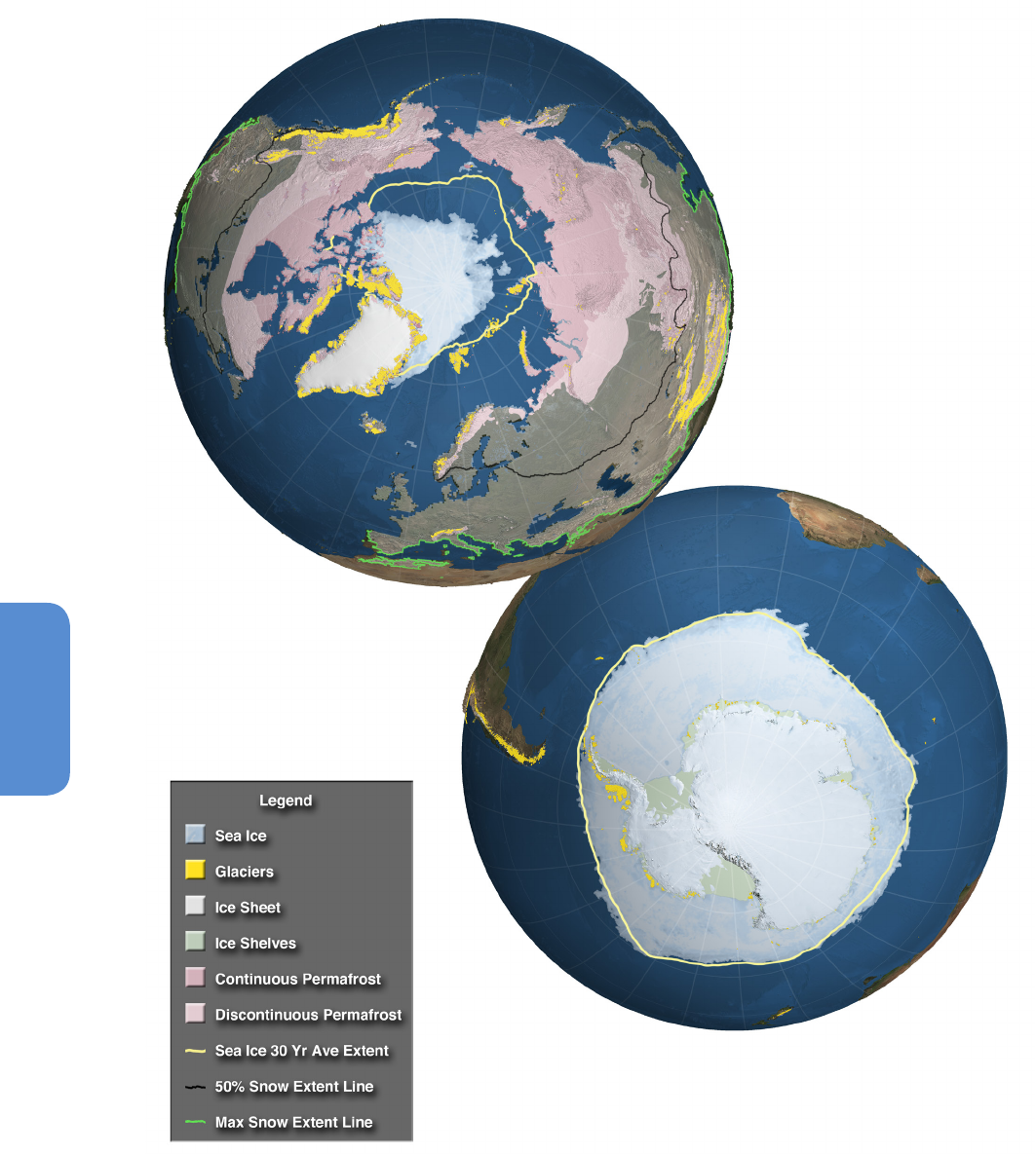
Figure 4.1 | The cryosphere in the Northern and Southern Hemispheres in polar projection. The map of the Northern Hemisphere shows the sea ice cover during minimum summer

extent (13 September 2012). The yellow line is the average location of the ice edge (15% ice concentration) for the yearly minima from 1979 to 2012. Areas of continuous perma-

frost (see Glossary) are shown in dark pink, discontinuous permafrost in light pink. The green line along the southern border of the map shows the maximum snow extent while

the black line across North America, Europe and Asia shows the 50% contour for frequency of snow occurrence. The Greenland ice sheet (blue/grey) and locations of glaciers (small

gold circles) are also shown. The map of the Southern Hemisphere shows approximately the maximum sea ice cover during an austral winter (13 September 2012). The yellow line

shows the average ice edge (15% ice concentration) during maximum extent of the sea ice cover from 1979 to 2012. Some of the elements (e.g., some glaciers and snow) located

at low latitudes are not visible in this projection (see Figure 4.8). The source of the data for sea ice, permafrost, snow and ice sheet are data sets held at the National Snow and Ice

Data Center (NSIDC), University of Colorado, on behalf of the North American Atlas, Instituto Nacional de Estadística, Geografía e Informática (Mexico), Natural Resources Canada,

U.S. Geological Survey, Government of Canada, Canada Centre for Remote Sensing and The Atlas of Canada. Glacier locations were derived from the multiple data sets compiled

in the Randolph Glacier Inventory (Arendt et al., 2012).

323

Observations: Cryosphere Chapter 4

changes in frozen ground (in particular, ice-rich permafrost) will

damage some vulnerable Arctic infrastructure (see WGII, Chapter 28),

and could substantially alter the carbon budget through the release of

methane (see Chapter 6).

Since AR4, substantial progress has been made in most types of cry-

ospheric observations. Satellite technologies now permit estimates

of regional and temporal changes in the volume and mass of the

ice sheets. The longer time series now available enable more accu-

rate assessments of trends and anomalies in sea ice cover and rapid

identiﬁcation of unusual events such as the dramatic decline of Arctic

summer sea ice extent in 2007 and 2012. Similarly, Arctic sea ice thick-

ness can now be estimated using satellite altimetry, allowing pan-Arc-

tic measurements of changes in volume and mass. A new global glacier

inventory includes nearly all glaciers (Arendt et al., 2012) (42% in AR4)

and allows for much better estimates of the total ice volume and its

past and future changes. Remote sensing measurements of regional

glacier volume change are also now available widely and modelling of

glacier mass change has improved considerably. Finally, ﬂuctuations in

the cryosphere in the distant and recent past have been mapped with

increasing certainty, demonstrating the potential for rapid ice loss,

compared to slow recovery, particularly when related to sea level rise.

This chapter describes the current state of the cryosphere and its indi-

vidual components, with a focus on recent improvements in under-

standing of the observed variability, changes and trends. Projections

of future cryospheric changes (e.g., Chapter 13) and potential drivers

(Chapter 10) are discussed elsewhere. Earlier IPCC reports used cry-

ospheric terms that have speciﬁc scientiﬁc meanings (see Cogley et

al., 2011), but have rather different meanings in everyday language.

To avoid confusion, this chapter uses the term ‘glaciers’ for what was

previously termed ‘glaciers and ice caps’ (e.g., Lemke et al., 2007). For

the two largest ice masses of continental size, those covering Green-

land and Antarctica, we use the term ‘ice sheets’. For simplicity, we use

units such as gigatonnes (Gt, 10

tonnes, or 10

kg). One gigatonne is

approximately equal to one cubic kilometre of freshwater (1.1 km

ice), and 362.5 Gt of ice removed from the land and immersed in the

oceans will cause roughly 1 mm of global sea level rise (Cogley, 2012).

4.2 Sea Ice

4.2.1 Background

Sea ice (see Glossary) is an important component of the climate

system. A sea ice cover on the ocean changes the surface albedo, insu-

lates the ocean from heat loss, and provides a barrier to the exchange

of momentum and gases such as water vapour and CO

between the

ocean and atmosphere. Salt ejected by growing sea ice alters the den-

sity structure and modiﬁes the circulation of the ocean. Regional cli-

mate changes affect the sea ice characteristics and these changes can

feed back on the climate system, both regionally and globally. Sea ice

is also a major component of polar ecosystems; plants and animals at

all trophic levels ﬁnd a habitat in, or are associated with, sea ice.

Most sea ice exists as pack ice, and wind and ocean currents drive the

drift of individual pieces of ice (called ﬂoes). Divergence and shear in

sea ice motion create areas of open water where, during colder months,

new ice can quickly form and grow. On the other hand, convergent ice

motion causes the ice cover to thicken by deformation. Two relatively

thin ﬂoes colliding with each other can ‘raft’, stacking one on top of

the other and thickening the ice. When thicker ﬂoes collide, thick ridges

may be built from broken pieces, with a height above the surface (ridge

sail) of 2 m or more, and a much greater thickness (~10 m) and width

below the ocean surface (ridge keel).

Sea ice thickness also increases by basal freezing during winter months.

But the thicker the ice becomes the more it insulates heat loss from the

ocean to the atmosphere and the slower the basal growth is. There is

an equilibrium thickness for basal ice growth that is dependent on the

surface energy balance and heat from the deep ocean below. Snow

cover lying on the surface of sea ice provides additional insulation, and

also alters the surface albedo and aerodynamic roughness. But also,

and particularly in the Antarctic, a heavy snow load on thin sea ice

can depress the ice surface and allow seawater to ﬂood the snow. This

saturated snow layer freezes quickly to form ‘snow ice’ (see FAQ 4.1).

Because sea ice is formed from seawater it contains sea salt, mostly

in small pockets of concentrated brine. The total salt content in newly

formed sea ice is only 25 to 50% of that in the parent seawater, and the

residual salt rejected as the sea ice forms alters ocean water density

and stability. The salinity of the ice decreases as it ages, and particu-

larly during the Arctic summer when melt water (including from melt

ponds that form on the surface) drains through and ﬂushes the ice.

The salinity and porosity of sea ice affect its mechanical strength, its

thermal properties and its electrical properties – the latter being very

important for remote sensing.

Geographical constraints play a dominant but not an exclusive role in

determining the quite different characteristics of sea ice in the Arctic

and the Antarctic (see FAQ 4.1). This is one of the reasons why changes

in sea ice extent and thickness are very different in the north and the

south. We also have much more information on Arctic sea ice thickness

than we do on Antarctic sea ice thickness, and so discuss Arctic and

Antarctic separately in this assessment.

4.2.2 Arctic Sea Ice

Regional sea ice observations, which span more than a century, have

revealed signiﬁcant interannual changes in sea ice coverage (Walsh

and Chapman, 2001). Since the advent of satellite multichannel pas-

sive microwave imaging systems in 1979, which now provide more

than 34 years of continuous coverage, it has been possible to monitor

the entire extent of sea ice with a temporal resolution of less than a

day. A number of procedures have been used to convert the observed

microwave brightness temperature into sea ice concentration— the

fractional area of the ocean covered by ice—and thence to derive sea

ice extent and area (Markus and Cavalieri, 2000; Comiso and Nishio,

2008). Sea ice extent is deﬁned as the sum of ice covered areas with

concentrations of at least 15%, while ice area is the product of the ice

concentration and area of each data element within the ice extent. A

brief description of the different techniques for deriving sea ice con-

centration is provided in the Supplementary Material. The trends in the

sea ice concentration, ice extent and ice area, as inferred from data

324

Chapter 4 Observations: Cryosphere

derived from the different techniques, are generally compatible. A com-

parison of derived ice extents from different sources is presented in the

next section and in the Supplementary Material. Results presented in

this assessment are based primarily on a single technique (Comiso and

Nishio, 2008) but the use of data from other techniques would provide

generally the same conclusions.

Arctic sea ice cover varies seasonally, with average ice extent varying

between about 6 × 10

in the summer and about 15 × 10

the winter (Comiso and Nishio, 2008; Cavalieri and Parkinson, 2012;

Meier et al., 2012). The summer ice cover is conﬁned to mainly the

Arctic Ocean basin and the Canadian Arctic Archipelago, while winter

sea ice reaches as far south as 44°N, into the peripheral seas. At the

end of summer, the Arctic sea ice cover consists primarily of the pre-

viously thick, old and ridged ice types that survived the melt period.

Interannual variability is largely determined by the extent of the ice

cover in the peripheral seas in winter and by the ice cover that survives

the summer melt in the Arctic Basin.

4.2.2.1 Total Arctic Sea Ice Extent and Concentration

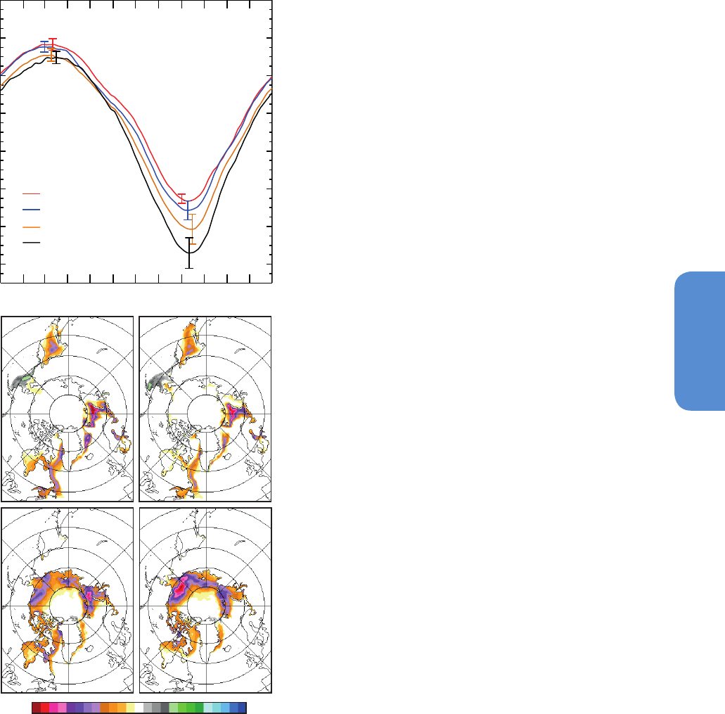
Figure 4.2 (derived from passive microwave data) shows both the sea-

sonality of the Arctic sea ice cover and the large decadal changes that

have occurred over the last 34 years. Typically, Arctic sea ice reaches

its maximum seasonal extent in February or March whereas the min-

imum occurs in September at the end of summer melt. Changes in

decadal averages in Arctic ice extent are more pronounced in summer

than in winter. The change in winter extent between 1979–1988 and

1989–1998 was negligible. Between 1989–1998 and 1999–2008,

there was a decrease in winter extent of around 0.6 × 10

. This

can be contrasted to a decrease in ice extent at the end of the summer

(September) of 0.5 × 10

between 1979–1988 and 1989–1998,

followed by a further decrease of 1.2 × 10

between 1989–1998

and 1999–2008. Figure 4.2 also shows that the change in extent from

1979–1988 to 1989–1998 was statistically signiﬁcant mainly in spring

and summer while the change from 1989–1998 to 1999–2008 was

statistically signiﬁcant during winter and summer. The largest inter-

annual changes occur during the end of summer when only the thick

components of the winter ice cover survive the summer melt (Comiso

et al., 2008; Comiso, 2012).

For comparison, the average extents during the 2009–2012 period are

also presented: the extent during this period was considerably less

than in earlier periods in all seasons, except spring. The summer min-

imum extent was at a record low in 2012 following an earlier record

set in 2007 (Stroeve et al., 2007; Comiso et al., 2008). The minimum

ice extent in 2012 was 3.44 × 10

while the low in 2007 was 4.22

× 10

. For comparison, the record high value was 7.86 × 10

in 1980. The low extent in 2012 (which is 18.5% lower than in 2007)

was probably caused in part by an unusually strong storm in the Cen-

tral Arctic Basin on 4 to 8 August 2012 (Parkinson and Comiso, 2013).

The extents for 2007 and 2012 were almost the same from June until

the storm period in 2012, after which the extent in 2012 started to

trend considerably lower than in 2007. The error bars, which represent

1 standard deviation (1σ) of samples used to estimate each data point,

are smallest in the ﬁrst decade and get larger with subsequent decades

indicating much higher interannual variability in recent years. The error

bars are also comparable in summer and winter during the ﬁrst decade

but become progressively larger for summer compared to winter in

subsequent decades. These results indicate that the largest interannual

variability has occurred in the summer and in the recent decade.

Although relatively short as a climate record, the 34-year satellite

record is long enough to allow determination of signiﬁcant and con-

sistent trends of the time series of monthly anomalies (i.e., difference

between the monthly and the averages over the 34-year record) of ice

extent, area and concentration. The trends in ice concentration for the

winter, spring, summer and autumn for the period November 1978 to

December 2012 are shown in Figure 4.2 (b, c, d and e). The seasonal

trends for different regions, except the Bering Sea, are negative. Ice

cover changes are relatively large in the eastern Arctic Basin and most

peripheral seas in winter and spring, while changes are pronounced

almost everywhere in the Arctic Basin, except at greater than 82°N, in

summer and autumn. In connection with a comprehensive observation-

al research program during the International Polar Year 2007–2008,

regional studies primarily on the Canadian side of the Arctic revealed

very similar patterns of spatial and interannual variability of the sea ice

cover (Derksen et al., 2012).

From the monthly anomaly data, the trend in sea ice extent in the

Northern Hemisphere (NH) for the period from November 1978 to

December 2012 is –3.8 ± 0.3% per decade (very likely) (see FAQ 4.1).

The error quoted is calculated from the standard deviation of the slope

of the regression line. The baseline for the monthly anomalies is the

average of all data for each month from November 1978 to December

2012. The trends for different regions vary greatly, ranging from +7.3%

per decade in the Bering Sea to –13.8% per decade in the Gulf of St.

Lawrence. This large spatial variability is associated with the complex-

ity of the atmospheric and oceanic circulation system as manifested in

the Arctic Oscillation (Thompson and Wallace, 1998). The trends also

differ with season (Comiso and Nishio, 2008; Comiso et al., 2011). For

the entire NH, the trends in ice extent are –2.3 ± 0.5%, –1.8 ± 0.5%,

–6.1 ± 0.8% and –7.0 ± 1.5% per decade (very likely) in winter, spring,

summer and autumn, respectively. The corresponding trends in ice area

are –2.8 ± 0.5%, –2.2 ± 0.5%, –7.2 ± 1.0%, and –7.8 ± 1.3% per

decade (very likely). Similar results were obtained by (Cavalieri and

Parkinson, 2012) but cannot be compared directly since their data are

for the period from 1979 to 2010 (see Supplementary Material). The

trends for ice extent and ice area are comparable except in the summer

and autumn, when the trend in ice area is signiﬁcantly more than that

in ice extent. This is due in part to increasing open water areas within

the pack that may be caused by more frequent storms and more diver-

gence in the summer (Simmonds et al., 2008). The trends are larger in

the summer and autumn mainly because of the rapid decline in the

multi-year ice cover (Comiso, 2012), as discussed in Section 4.2.2.3.

The trends in km

–1

were estimated as in Comiso and Nishio (2008)

and Comiso (2012) but the percentage trends presented in this chapter

were calculated differently. Here the percentage is calculated as a dif-

ference from the ﬁrst data point on the trend line whereas the earlier

estimations used the difference from the mean value. The new percent-

age trends are only slightly different from the previous ones and the

conclusions about changes are the same.

325

Observations: Cryosphere Chapter 4

terrestrial proxies (e.g., Macias Fauria et al., 2010; Kinnard et al., 2011).

The records constructed by Kinnard et al. (2011) and Macias Fauria et

al. (2010) suggest that the decline of sea ice over the last few decades

has been unprecedented over the past 1450 years (see Section 5.5.2).

In a study of the marginal seas near the Russian coastline using ice

extent data from 1900 to 2000, Polyakov et al. (2003) found a low

frequency multi-decadal oscillation near the Kara Sea that shifted to a

dominant decadal oscillation in the Chukchi Sea.

A more comprehensive basin-wide record, compiled by Walsh and

Chapman (2001), showed very little interannual variability until the

last three to four decades. For the period 1901 to 1998, their results

show a summer mode that includes an anomaly of the same sign over

nearly the entire Arctic and that captures the sea-ice trend from recent

satellite data. Figure 4.3 shows an updated record of the Walsh and

Chapman data set with longer time coverage (1870 to 1978) that is

more robust because it includes additional historical sea ice observa-

tions (e.g., from Danish meteorological stations). A comparison of this

updated data set with that originally reported by Walsh and Chapman

(2001) shows similar interannual variability that is dominated by a

nearly constant extent of the winter (January–February–March) and

autumn (October–November–December) ice cover from 1870 to the

1950s. The absence of interannual variability during that period is due

to the use of climatology to ﬁll gaps, potentially masking the natural

signal. Sea ice data from 1900–2011 as compiled by Met Ofﬁce Hadley

Centre are also plotted for comparison. In this data set, the 1979–2011

values were derived from various sources, including satellite data, as

described by Rayner et al. (2003). Since the 1950s, more in situ data are

available and have been homogenized with the satellite record (Meier

et al., 2012). These data show a consistent decline in the sea ice cover

that is relatively moderate during the winter but more dramatic during

the summer months. Satellite data from other sources are also plotted

in Figure 4.3, including Scanning Multichannel Microwave Radiome-

ter (SMMR) and Special Sensor Microwave/Imager (SSM/I) data using

the Bootstrap Algorithm (SBA) as described by Comiso and Nishio

(2008) and National Aeronautics and Space Administration (NASA)

Team Algorithm (NT1) as described by Cavalieri et al. (1984) (see Sup-

plementary Material). Data from the Advanced Microwave Scanning

Radiometer - Earth Observing System (AMSR-E) using the Bootstrap

Algorithm (ABA) and the NASA Team Algorithm Version 2 (NT2) are

also presented. The error bars represent one standard deviation of the

interannual variability during the satellite period. Because of the use of

climatology to ﬁll data gaps from 1870 to 1953, the error bars in the

Walsh and Chapman data were set to twice that of the satellite period

and 1.5 times higher for 1954 to 1978. The apparent reduction of the

sea ice extent from 1978 to 1979 is in part due to the change from

surface observations to satellite data. Generally, the temporal distri-

butions from the various sources are consistent with some exceptions

that may be attributed to possible errors in the data (e.g., Screen, 2011

and Supplementary Material). Taking this into account, the various

sources provide similar basic information and conclusions about the

changing extent and variability of the Arctic sea ice cover.

4.2.2.3 Multi-year/Seasonal Ice Coverage

The winter extent and area of the perennial and multi-year ice cover

in the Central Arctic (i.e., excluding Greenland Sea multi-year ice) for

Figure 4.2 | (a) Plots of decadal averages of daily sea ice extent in the Arctic (1979 to

1988 in red, 1989 to 1998 in blue, 1999 to 2008 in gold) and a 4-year average daily

ice extent from 2009 to 2012 in black. Maps indicate ice concentration trends (1979–

2012) in (b) winter, (c) spring, (d) summer and (e) autumn (updated from Comiso, 2010).

a) Daily ice extent

JFMAMJJASOND

Ice extent (10

)

1979-1988

1989-1998

1999-2008

2009-2012

b) Winter (DJF)

c) Spring (MAM)

d) Summer (JJA)

e) Autumn (SON)

-2.4 -1.6 -0.8 0.0 0.8 1.6 2.4

Trend (% IC yr

-1

)

4.2.2.2 Longer Records of Arctic Ice Extent

For climate analysis, the variability of the sea ice cover prior to the

commencement of the satellite record in 1979 is also of interest. There

are a number of pre-satellite records, some based on regional obser-

vations taken from ships or aerial reconnaissance (e.g., Walsh and

Chapman, 2001; Polyakov et al., 2003) while others were based on

326

Chapter 4 Observations: Cryosphere

1979–2012 are shown in Figure 4.4. Perennial ice is that which survives

the summer, and the ice extent at summer minimum has been used as

a measure of its coverage (Comiso, 2002). Multi-year ice (as deﬁned

by World Meteorological Organization) is ice that has survived at least

two summers. Generally, multi-year ice is less saline and has a distinct

microwave signature that differs from the seasonal ice, and thus can

be discriminated and monitored with satellite microwave radiometers

(Johannessen et al., 1999; Zwally and Gloersen, 2008; Comiso, 2012).

Figure 4.4 shows similar interannual variability and large trends for

both perennial and multi-year ice for the period 1979 to 2012. The

extent of the perennial ice cover, which was about 7.9 × 10

1980, decreased to as low as 3.5 × 10

in 2012. Similarly, the

multi-year ice extent decreased from about 6.2 × 10

in 1981 to

about 2.5 × 10

in 2012. The trends in perennial ice extent and

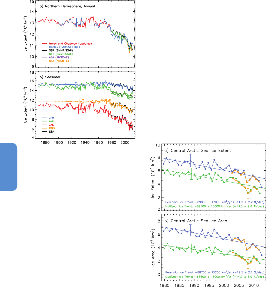
Figure 4.3 | Ice extent in the Arctic from 1870 to 2011. (a) Annual ice extent and (b)

seasonal ice extent using averages of mid-month values derived from in situ and other

sources including observations from the Danish meteorological stations from 1870 to

1978 (updated from, Walsh and Chapman, 2001). Ice extent from a joint Hadley and

National Oceanic and Atmospheric Administration (NOAA) project (called HADISST1_

Ice) from 1900 to 2011 is also shown. The yearly and seasonal averages for the period

from 1979 to 2011 are shown as derived from Scanning Multichannel Microwave Radi-

ometer (SMMR) and Special Sensor Microwave/Imager (SSM/I) passive microwave data

using the Bootstrap Algorithm (SBA) and National Aeronautics and Space Administra-

tion (NASA) Team Algorithm, Version 1 (NT1), using procedures described in Comiso and

Nishio (2008), and Cavalieri et al. (1984), respectively; and from Advanced Microwave

Scanning Radiometer, Version 2 (AMSR2) using algorithms called AMSR Bootstrap Algo-

rithm (ABA) and NASA Team Algorithm, Version 2 (NT2), described in Comiso and Nishio

(2008) and Markus and Cavalieri (2000). In (b), data from the different seasons are

shown in different colours to illustrate variation between seasons, with SBA data from

the procedure in Comiso and Nishio (2008) shown in black.

Figure 4.4 | Annual perennial (blue) and multi-year (green) sea ice extent (a) and sea

ice area (b) in the Central Arctic from 1979 to 2012 as derived from satellite passive

microwave data (updated from Comiso, 2012). Perennial ice values are derived from

summer minimum ice extent, while the multi-year ice values are averages of those from

December, January and February. The gold lines (after 2002) are from AMSR-E data.

Uncertainties in the observations (very likely range) are indicated by representative error

bars, and uncertainties in the trends are given (very likely range).

ice area were strongly negative at –11.5 ± 2.1 and –12.5 ± 2.1% per

decade (very likely) respectively. These values indicate an increased

rate of decline from the –6.4% and –8.5% per decade, respectively,

reported for the 1979 to 2000 period by Comiso (2002). The trends in

multi-year ice extent and area are even more negative, at –13.5 ± 2.5

and –14.7 ± 3.0% per decade (very likely), respectively, as updated for

the period 1979 to 2012 (Comiso, 2012). The more negative trend in ice

area than in ice extent indicates that the average ice concentration of

multi-year ice in the Central Arctic has also been declining. The rate of

decline in the extent and area of multi-year ice cover is consistent with

the observed decline of old ice types from the analysis of ice drift and

ice age by Maslanik et al. (2007), conﬁrming that older and thicker ice

types in the Arctic have been declining signiﬁcantly. The more negative

trend for the thicker multi-year ice area than that for the perennial ice

area implies that the average thickness of the ice, and hence the ice

volume, has also been declining.

Drastic changes in the multi-year ice coverage from QuikScat (satellite

radar scatterometer) data, validated using high-resolution Synthetic

Aperture Radar data (Kwok, 2004; Nghiem et al., 2007), have also been

reported. Some of these changes have been attributed to the near zero

replenishment of the Arctic multi-year ice cover by ice that survives the

summer (Kwok, 2007).

327

Observations: Cryosphere Chapter 4

4.2.2.4 Ice Thickness and Volume

For the Arctic, there are several techniques available for estimating

the thickness distribution of sea ice. Combined data sets of draft and

thickness from submarine sonars, satellite altimetry and airborne elec-

tromagnetic sensing provide broadly consistent and strong evidence of

decrease in Arctic sea ice thickness in recent years (Figure 4.6c).

Data collected by upward-looking sonar on submarines operating

beneath the Arctic pack ice provided the ﬁrst evidence of ‘basin-wide’

decreases in ice thickness (Wadhams, 1990). Sonar measurements are

of average draft (the submerged portion of sea ice), which is converted

to thickness by assuming an average density for the measured ﬂoe

including its snow cover. With the then available submarine records,

Rothrock et al. (1999) found that ice draft in the mid-1990s was less

than that measured between 1958 and 1977 in each of six regions

within the Arctic Basin. The change was least (–0.9 m) in the Beau-

fort and Chukchi seas and greatest (–1.7 m) in the Eurasian Basin. The

decrease averaged about 42% of the average 1958 to 1977 thickness.

This decrease matched the decline measured in the Eurasian Basin

between 1976 and 1996 using UK submarine data (Wadhams and

Davis, 2000), which was 43%.

A subsequent analysis of US Navy submarine ice draft (Rothrock et

al., 2008) used much richer and more geographically extensive data

from 34 cruises within a data release area that covered almost 38%

of the area of the Arctic Ocean. These cruises were equally distributed

in spring and autumn over a 25-year period between 1975 and 2000.

Observational uncertainty associated with the ice draft from these is

0.5 m (Rothrock and Wensnahan, 2007). Multiple regression analysis

was used to separate the interannual changes (Figure 4.6c), the annual

cycle and the spatial distribution of draft in the observations. Results of

that analysis show that the annual mean ice thickness declined from a

peak of 3.6 m in 1980 to 2.4 m in 2000, a decrease of 1.2 m. Over the

period, the most rapid change was –0.08 m yr

–1

in 1990.

The most recent submarine record, Wadhams et al. (2011), found that

tracks north of Greenland repeated between the winters of 2004 and

2007 showed a continuing shift towards less multi-year ice.

Satellite altimetry techniques are now capable of mapping sea ice free-

board to provide relatively comprehensive pictures of the distribution

of Arctic sea ice thickness. Similar to the estimation of sea ice thick-

ness from ice draft, satellite measured freeboard (the height of sea ice

above the water surface) is converted to thickness, assuming an aver-

age density of ice and snow. The principal challenges to accurate thick-

ness estimation using satellite altimetry are in the discrimination of

ice and open water, and in estimating the thickness of the snow cover.

Since 1993, radar altimeters on the European Space Agency (ESA),

European Remote Sensing (ERS) and Envisat satellites have provided

Arctic observations south of 81.5°N. With the limited latitudinal reach

of these altimeters, however, it has been difﬁcult to infer basin-wide

changes in thickness. The ERS-1 estimates of ice thickness show a

downward trend but, because of the high variability and short time

series (1993–2001), Laxon et al. (2003) concluded that the trend in a

region of mixed seasonal and multi-year ice (i.e., below 81.5°N) cannot

be considered as signiﬁcant. Envisat observations showed a large

decrease in thickness (0.25 m) following September 2007 when ice

extent was the second lowest on record (Giles et al., 2008b). This was

associated with the large retreat of the summer ice cover, with thinning

regionally conﬁned to the Beaufort and Chukchi seas, but with no sig-

niﬁcant changes in the eastern Arctic. These results are consistent with

those from the NASA Ice, Cloud and land Elevation Satellite (ICESat)

laser altimeter (see comment on ICESat data in Section 4.4.2.1), which

show thinning in the same regions between 2007 and 2008 (Kwok,

2009) (Figure 4.5). Large decreases in thickness due to the 2007 mini-

mum in summer ice are clearly seen in both the radar and laser altim-

eter thickness estimates.

The coverage of the laser altimeter on ICESat (which ceased opera-

tion in 2009) extended to 86°N and provided a more complete spatial

pattern of the thickness distribution in the Arctic Basin (Figure 4.6c).

Thickness estimates are consistently within 0.5 m of sonar measure-

ments from near-coincident submarine tracks and proﬁles from sonar

moorings in the Chukchi and Beaufort seas (Kwok, 2009). Ten ICESat

campaigns between autumn 2003 and spring 2008 showed seasonal

differences in thickness and thinning and volume losses of the Arctic

Ocean ice cover (Kwok, 2009). Over these campaigns, the multi-year

sea ice thickness in spring declined by ~0.6 m (Figure 4.5), while the

average thickness of the ﬁrst-year ice (~2 m) had a negligible trend.

The average sea ice volume inside the Arctic Basin in spring (February/

March) was ~14,000 km

. Between 2004 and 2008, the total multi-year

ice volume in spring (February/March) experienced a net loss of 6300

(>40%). Residual differences between sonar mooring and satellite

thicknesses suggest basin-scale volume uncertainties of approximate-

ly 700 km

. The rate of volume loss (–1237 km

–1

) during autumn

(October/November), while highlighting the large changes during the

short ICESat record compares with a more moderate loss rate (–280

± 100 km

–1

) over a 31-year period (1979–2010) estimated from a

sea ice reanalysis study using the Pan-Arctic Ice-Ocean Modelling and

Assimilation system (Schweiger et al., 2011).

The CryoSat-2 radar altimeter (launched in 2010), which provides cov-

erage up to 89°N, has provided new thickness and volume estimates

of Arctic Ocean sea ice (Laxon et al., 2013). These show that the ice

volume inside the Arctic Basin decreased by a total of 4291 km

autumn (October/November) and 1479 km

in winter (February/March)

between the ICESat (2003–2008) and CryoSat-2 (2010–2012) periods.

Based on ice thickness estimates from sonar moorings, an inter-satel-

lite bias between ICESat and CryoSat-2 of 700 km

can be expected.

This is much less than the change in volume between the two periods.

Airborne electro-magnetic (EM) sounding measures the distance

between an EM instrument near the surface or on an aircraft and the

ice/water interface, and provides another method to measure ice thick-

ness. Uncertainties in these thickness estimates are 0.1 m over level

ice. Comparison with drill-hole measurements over a mix of level and

ridged ice found differences of 0.17 m (Haas et al., 2011).

Repeat EM surveys in the Arctic, though restricted in time and space,

have provided a regional view of the changing ice cover. From repeat

ground-based and helicopter-borne EM surveys, Haas et al. (2008)

found signiﬁcant thinning in the region of the Transpolar Drift (an

328

Chapter 4 Observations: Cryosphere

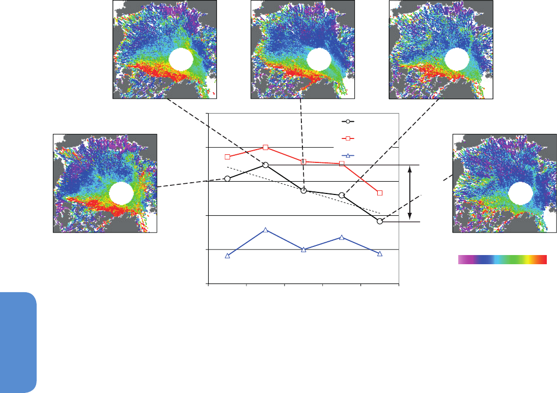
Figure 4.5 | The distribution of winter sea ice thickness in the Arctic and the trends in average, ﬁrst-year (FY and multi-year (MY) ice thickness derived from ICESat data between

2004 and 2008 (Kwok, 2009).

FM06

MA07

FM08

Thickness (m)

0.0 5.0

1.5

2.0

2.5

3.0

3.5

4.0

Overall

MY ice

FY ice

2004 2005 2006 2007 2008

Thickness (m)

Trend = -0.17± 0.05 m yr

-1

Greenland

2005

Greenland

2006

Greenland

2007

Greenland

2008

Greenland

2004

Greenland

0.83 m

average wind-driven drift pattern that transports sea ice from the Sibe-

rian coast of Russia across the Arctic Basin to Fram Strait). Between

1991 and 2004, the modal ice thickness decreased from 2.5 m to 2.2

m, with a larger decline to 0.9 m in 2007. Mean ice thicknesses also

decreased strongly. This thinning was associated with reduction of the

age of the ice, and replacement of second-year ice by ﬁrst-year ice in

2007 (following the large decline in summer ice extent in 2007) as

seen in satellite observations. Ice thickness estimates from EM surveys

near the North Pole can be compared to submarine estimates (Figure

4.6c). Airborne EM measurements from the Lincoln Sea between 83°N

and 84°N since 2004 (Haas et al., 2010) showed some of the thickest

ice in the Arctic, with mean and modal thicknesses of more than 4.5 m

and 4 m, respectively. Since 2008, the modal thickness in this region

has declined to 3.5 m, which is most likely related to the narrowing

of the remaining band of old ice along the northern coast of Canada.

4.2.2.5 Arctic Sea Ice Drift

Ice motion inﬂuences the distribution of sea ice thickness in the Arctic

Basin: locally, through deformation and creation of open water areas;

regionally, through advection of ice from one area to another; and

basin-wide, through export of ice from polar seas to lower latitudes

where it melts. The drift and deformation of sea ice is forced primarily

by winds and surface currents, but depends also on ice strength, top

and bottom surface roughness, and ice concentration. On time scales

of days to weeks, winds are responsible for most of the variance in sea

ice motion.

Drifting buoys have been used to measure Arctic sea ice motion since

1979. From the record of buoy drift archived by the International Arctic

Buoy Programme, Rampal et al. (2009) found an increase in average

drift speed between 1978 and 2007 of 17 ± 4.5% per decade in winter

and 8.5 ± 2.0% per decade in summer. Using daily satellite ice motion

ﬁelds, which provide a basin-wide picture of the ice drift, Spreen et

al. (2011) found that, between 1992 and 2008, the spatially averaged

winter ice drift speed increased by 10.6 ± 0.9% per decade, but varied

regionally between −4 and +16% per decade (Figure 4.6d). Increases

in drift speed are seen over much of the Arctic except in areas with

thicker ice (Figure 4.6b, e.g., north of Greenland and the Canadian

Archipelago). The largest increases occurred during the second half of

the period (2001–2009), coinciding with the years of rapid ice thinning

discussed in Section 4.2.2.4. Both Rampal et al. (2009) and Spreen et al.

(2011) suggest that, since atmospheric reanalyses do not show strong-

er winds, the positive trend in drift speed is probably due to a weaker

and thinner ice cover, especially during the period after 2003.

In addition to freezing and melting, sea ice export through Fram Strait

is a major component of the Arctic Ocean ice mass balance. Approxi-

mately10% of the area of Arctic Ocean ice is exported annually. Over a

32-year satellite record (1979–2010), the mean annual outﬂow of ice

area through Fram Strait was 699 ± 112 × 10

with a peak during

the 1994–1995 winter (updated from , Kwok, 2009), but with no sig-

niﬁcant decadal trend. Decadal trends in ice volume export—a more

deﬁnitive measure of change—is far less certain owing to the lack of

an extended record of the thickness of sea ice exported through Fram

329

Observations: Cryosphere Chapter 4

Strait. Comparison of volume outﬂow using ICESat thickness estimates

(Spreen et al., 2009) with earlier estimates by Kwok and Rothrock

(1999) and Vinje (2001) using thicknesses from moored upward look-

ing sonars shows no discernible change.

Between 2005 and 2008, more than a third of the thicker and older sea

ice loss occurred by transport of thick, multi-year ice, typically found

west of the Canadian Archipelago, into the southern Beaufort Sea,

where it melted in summer (Kwok and Cunningham, 2010). Uncertain-

ties remain in the relative contributions of in-basin melt and export to

observed changes in Arctic ice volume loss, and it has also been shown

that export of thicker ice through Nares Strait could account for a small

fraction of the loss (Kwok, 2005).

4.2.2.6 Timing of Sea Ice Advance, Retreat and Ice Season

Duration; Length of Melt Season

Importantly from both physical and biological perspectives, strong

regional changes have occurred in the seasonality of sea ice in both

polar regions (Massom and Stammerjohn, 2010; Stammerjohn et al.,

2012). However, there are distinct regional differences in when sea-

sonally the change is strongest (Stammerjohn et al., 2012).

Seasonality collectively describes the annual time of sea ice advance

and retreat, and its duration (the time between day of advance and

retreat). Daily satellite ice-concentration records (1979–2012) are used

to determine the day to which sea ice advanced, and the day from

which it retreated, for each satellite pixel location. Maps of the timing of

sea ice advance, retreat and duration are derived from these data (see

Parkinson (2002) and Stammerjohn et al. (2008) for detailed methods).

Most regions in the Arctic show trends towards shorter ice season

duration. One of the most rapidly changing areas (showing great-

er than 2 days yr

–1

change) extends from the East Siberian Sea to

the western Beaufort Sea. Here, between 1979 and 2011, sea ice

advance occurred 41 ± 6 days later (or 1.3 ± 0.2 days yr

–1

), sea

ice retreat 49 ± 7 days earlier (–1.5 ± 0.2 days yr

–1

), and duration

became 90 ± 16 days shorter (–2.8 ± 0.5 days yr

–1

) (Stammerjohn

et al., 2012). This 3-month lengthening of the summer ice-free season

places Arctic summer sea ice extent loss into a seasonal perspective

and underscores impacts to the marine ecosystem (e.g., Grebmeier et

al., 2010).

The timing of surface melt onset in spring, and freeze-up in autumn,

can be derived from satellite microwave data as the emissivity of the

surface changes signiﬁcantly with snow melt (Smith, 1998; Drobot and

Anderson, 2001; Belchansky et al., 2004). The amount of solar energy

absorbed by the ice cover increases with the length of the melt season.

Longer melt seasons with lower albedo surfaces (wet snow, melt ponds

and open water) increase absorption of incoming shortwave radiation

and ice melt (Perovich et al., 2007). Hudson (2011) estimates that the

observed reduction in Arctic sea ice has contributed approximately

0.1 W m

–2

of additional global radiative forcing, and that an ice-free

summer Arctic Ocean will result in a forcing of about 0.3 W m

–2

. The

satellite record (Markus et al., 2009) shows a trend toward earlier melt

and later freeze-up nearly everywhere in the Arctic (Figure 4.6e). Over

the last 34 years, the mean melt season over the Arctic ice cover has

increased at a rate of 5.7 ± 0.9 days per decade. The largest and most

signiﬁcant trends (at the 99% level) of more than 10 days per decade

are seen in the coastal margins and peripheral seas: Hudson Bay, the

East Greenland Sea, the Laptev/East Siberian seas, and the Chukchi/

Beaufort seas.

4.2.2.7 Arctic Polynyas

High sea ice production in coastal polynyas (anomalous regions of

open water or low ice concentration) over the continental shelves of

the Arctic Ocean is responsible for the formation of cold saline water,

which contributes to the maintenance of the Arctic Ocean halocline

(see Glossary). A new passive microwave algorithm has been used to

estimate thin sea ice thicknesses (<0.15 m) in the Arctic Ocean (Tamura

and Ohshima, 2011), providing the ﬁrst circumpolar mapping of sea ice

production in coastal polynyas. High sea ice production is conﬁned to

the most persistent Arctic coastal polynyas, with the highest ice pro-

duction rate being in the North Water Polynya. The mean annual sea ice

production in the 10 major Arctic polynyas is estimated to be 2942 ±

373 km

and decreased by 462 km

between 1992 and 2007 (Tamura

and Ohshima, 2011).

4.2.2.8 Arctic Land-Fast Ice

Shore- or land-fast ice is sea ice attached to the coast. Land-fast ice

along the Arctic coast is usually grounded in shallow water, with the

seaward edge typically around the 20 to 30 m isobath (Mahoney et al.,

2007). In fjords and conﬁned bays, land-fast ice extends into deeper

water.

There are no reliable estimates of the total area or interannual variabil-

ity of land-fast ice in the Arctic. However, both signiﬁcant and non-sig-

niﬁcant trends have been observed regionally. Long-term monitoring

near Hopen, Svalbard, revealed thinning of land-fast ice in the Barents

Sea region by 11 cm per decade between 1966 and 2007 (Gerland et

al., 2008). Between 1936 and 2000, the trends in land-fast ice thick-

ness (in May) at four Siberian sites (Kara Sea, Laptev Sea, East Siberi-

an Sea, Chukchi Sea) are insigniﬁcant (Polyakov et al., 2003). A more

recent composite time series of land-fast ice thickness between the

mid 1960s and early 2000s from 15 stations along the Siberian coast

revealed an average rate of thinning of 0.33 cm yr

–1

(Polyakov et al.,

2010). End-of-winter ice thickness for three stations in the Canadian

Arctic reveal a small downward trend at Eureka, a small positive trend

at Resolute Bay, and a negligible trend at Cambridge Bay (updated

from Brown and Coté, 1992; Melling, 2012), but these trends are small

and not statistically signiﬁcant. Even though the trend in the land-fast

ice extent near Barrow, Alaska has not been signiﬁcant (Mahoney et

al., 2007), relatively recent observations by Mahoney et al. (2007) and

Druckenmiller et al. (2009) found longer ice-free seasons and thinner

land-fast ice compared to earlier records (Weeks and Gow, 1978; Barry

et al., 1979). As freeze-up happens later, the growth season shortens

and the thinner ice breaks up and melts earlier.

4.2.2.9 Decadal Trends in Arctic Sea Ice

The average decadal extent of Arctic sea ice has decreased in every

season and in every successive decade since satellite observations

330

Chapter 4 Observations: Cryosphere

commenced. The data set is robust with continuous and consistent

global coverage on a daily basis thereby providing very reliable trend

results (very high conﬁdence). The annual Arctic sea ice cover very

likely declined within the range 3.5 to 4.1% per decade (0.45 to 0.51

million km

per decade) during the period 1979–2012 with larger

changes occurring in summer and autumn (very high conﬁdence).

Much larger changes apply to the perennial ice (the summer minimum

extent) which very likely decreased in the range from 9.4 % to 13.6 %

per decade (0.73 to 1.07 million km

per decade) and multiyear sea ice

(more than 2 years old) which very likely declined in the range from

11.0 % to 16.0% per decade (0.66 to 0.98 million km

per decade)

(very high conﬁdence; Figure 4.4b). The rate of decrease in ice area

has been greater than that in extent (Figure 4.4b) because the ice con-

centration has also decreased. The decline in multiyear ice cover as

observed by QuikScat from 1992 to 1910 is presented in Figure 4.6b

and shown to be consistent with passive microwave data (Figure 4.4b).

The decrease in perennial and multi-year ice coverage has resulted in a

strong decrease in ice thickness, and hence in ice volume. Declassiﬁed

submarine sonar measurements, covering ~38% of the Arctic Ocean,

indicate an overall mean winter thickness of 3.64 m in 1980, which

likely decreased by 1.8 [1.3 to 2.3] m by 2008 (high conﬁdence, Figure

4.6c). Between 1975 and 2000, the steepest rate of decrease was 0.08

m yr

–1

in 1990 compared to a slightly higher winter/summer rate of

0.10/0.20 m yr

–1

in the 5-year ICESat record (2003–2008). This com-

bined analysis (Figure 4.6c) shows a long-term trend of sea ice thinning

that spans ﬁve decades. Satellite measurements made in the period

2010–2012 show a decrease in basin-scale sea ice volume compared

to those made over the period 2003–2008 (medium conﬁdence). The

Arctic sea ice is becoming increasingly seasonal with thinner ice, and it

will take several years for any recovery.

The decreases in both concentration and thickness reduces sea ice

strength reducing its resistance to wind forcing, and drift speed has

increased (Figure 4.6d) (Rampal et al., 2009; Spreen et al., 2011). Other

signiﬁcant changes to the Arctic Ocean sea ice include lengthening in

the duration of the surface melt on perennial ice of 6 days per decade

(Figure 4.6e) and a nearly 3-month lengthening of the ice-free season

in the region from the East Siberian Sea to the western Beaufort Sea.

4.2.3 Antarctic Sea Ice

The Antarctic sea ice cover is largely seasonal, with average extent var-

ying from a minimum of about 3 × 10

in February to a maximum

of about 18 × 10

in September (Zwally et al., 2002a; Comiso et al.,

2011). The relatively small fraction of Antarctic sea ice that survives the

summer is found mostly in the Weddell Sea, but with some perennial

ice also surviving on the western side of the Antarctic Peninsula and

in small patches around the coast. As well as being mostly ﬁrst-year

ice, Antarctic sea ice is also on average thinner, warmer, more saline

and more mobile than Arctic ice (Wadhams and Comiso, 1992). These

characteristics, which reduce the capabilities of some remote sensing

techniques, together with its more distant location from inhabited con-

tinents, result in far less being known about the properties of Antarctic

sea ice than of that in the Arctic.

4.2.3.1 Total Antarctic Sea Ice Extent and Concentration

Figure 4.7a shows the seasonal variability of Antarctic sea ice extent

using 34 years of satellite passive microwave data updated from

Comiso and Nishio (2008). In contrast to the Arctic, decadal monthly

averages almost overlap with each other, and the seasonal variability

of the total Antarctic sea ice cover has not changed much over the

period. In winter, the values for the 1999–2008 decade were slightly

higher than those of the other decades; whereas in autumn the values

for 1989–1998 and 1999–2008 decades were higher than those of

1979–1988. There was more seasonal variability in the period 2009–

2012 than for earlier decadal periods, with relatively high values in late

autumn, winter and spring.

Trend maps for winter, spring, summer and autumn extent are present-

ed in Figure 4.7 (b, c, d and e respectively). The seasonal trends are sig-

niﬁcant mainly near the ice edge, with the values alternating between

positive and negative around Antarctica. Such an alternating pattern is

similar to that described previously as the Antarctic Circumpolar Wave

(ACW) (White and Peterson, 1996) but the ACW may not be associated

with the trends because the trends have been strongly positive in the

Ross Sea and negative in the Bellingshausen/Amundsen seas but with

almost no trend in the other regions (Comiso et al., 2011). In the winter,

negative trends are evident at the tip of the Antarctic Peninsula and

the western part of the Weddell Sea, while positive trends are prev-

alent in the Ross Sea. The patterns in spring are very similar to those

of winter, whereas in summer and autumn negative trends are mainly

conﬁned to the Bellingshausen/Amundsen seas, while positive trends

are dominant in the Ross Sea and the Weddell Sea.

The regression trend in the monthly anomalies of Antarctic sea ice

extent from November 1978 to December 2012 (updated from Comiso

and Nishio, 2008) is slightly positive, at 1.5 ± 0.3% per decade, or 0.13

to 0.20 million km

per decade (very likely) (see FAQ 4.1). The seasonal

trends in ice extent are 1.2 ± 0.5%, 1.0 ± 0.5%, 2.5 ± 2.0% and 3.0

± 2.0% per decade (very likely) in winter, spring, summer and autumn,

respectively, as updated from Comiso et al. (2011). The corresponding

trends in ice area (also updated) are 1.9 ± 0.7%, 1.6 ± 0.5%, 3.0 ±

2.1%, and 4.4 ± 2.3% per decade (very likely). The values are all pos-

itive, with the largest trends occurring in the autumn. The trends are

consistently higher for ice area than ice extent, indicating less open

water (possibly due to less storms and divergence) within the pack in

later years. Trends reported by Parkinson and Cavalieri (2012) using

data from 1978 to 2010 are slightly different, in part because they

cover a different time period (see Supplementary Material). The overall

interannual trends for various sectors around Antarctica are given in

FAQ 4.1, and show large regional variability. Changes in ice drift and

wind patterns as reported by Holland and Kwok (2012) may be related

to this phenomenon.

4.2.3.2 Antarctic Sea Ice Thickness and Volume

Since AR4, some advances have been made in determining the thick-

ness of Antarctic sea ice, particularly in the use of ship-based obser-

vations and satellite altimetry. However, there is still no information

on large-scale Antarctic ice thickness change. Worby et al. (2008)

compiled 25 years of ship-based data from 83 Antarctic voyages on

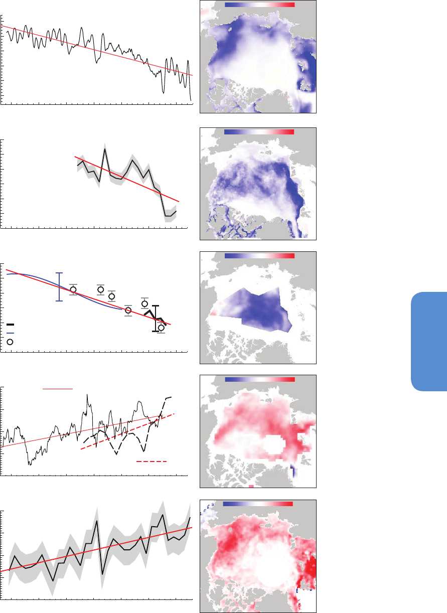
331

Observations: Cryosphere Chapter 4

1980 1985 1990 1995 2000 2005 2010

1.0

1.5

2.0

2.5

3.0

3.5

4.0

Ice thickness (m)

-0.62 (m per decade)

c) Ice thickness

EM surveys (North Pole)

Regression of submarine observations

Winter

Thickness

ICESat

-1.0 0.0(m per decade)

1980 1985 1990 1995 2000 2005 2010

2.0

2.5

3.0

3.5

4.0

4.5

5.0

MYice area (10

)

-0.80±0.2 x10

(km

per decade)

b) Multiyear ice coverage (Jan-1)

Multiyear ice concentration

-50.0 50.0 (% per decade)

1980 1985 1990 1995 2000 2005 2010

-2

-1

Sea ice drift speed

anomaly (km day

-1

)

Satellite ice drift (Oct-May):

0.94

±0.3

(km day

-1

per decade)

d) Sea ice drift speed

Drift speed

Buoy drift:

0.55±0.04 (km day

-1

per decade)

-2.5 2.5(km day

-1

per decade)

Length of melt (day)

e) Average length of melt season

Length of melt season

-30.0 30.0

(day per decade)

5.7±0.9 (day per decade)

1980 1985 1990 1995 2000 2005 2010

100

110

120

130

Ice extent

anomaly (10

)

-3.8±0.3 (% per decade)

a) Annual ice extent

Ice concentration

-10.0 10.0 (% per decade)

1980 1985 1990 1995 2000 2005 2010

-1.0

-0.5

0.0

0.5

1.0

-1.5

Figure 4.6 | Summary of linear decadal trends (red lines) and pattern of changes in the following: (a) Anomalies in Arctic sea ice extent from satellite passive microwave observa-

tions (Comiso and Nishio, 2008, updated to include 2012). Uncertainties are discussed in the text. (b) Multi-year sea ice coverage on January 1st from analysis of the QuikSCAT

time series (Kwok, 2009); grey band shows uncertainty in the retrieval. (c) Sea ice thickness from submarine (blue), satellites (black) (Kwok and Rothrock, 2009), and in situ/electro-

magnetic (EM) surveys (circles) (Haas et al., 2008); trend in submarine ice thickness is from multiple regression of available observations within the data release area (Rothrock et

al., 2008). Error bars show uncertainties in observations. (d) Anomalies in buoy (Rampal et al., 2009) and satellite-derived sea ice drift speed (Spreen et al., 2011). (e) Length of melt

season (updated from Markus et al., 2009); grey band shows the basin-wide variability.

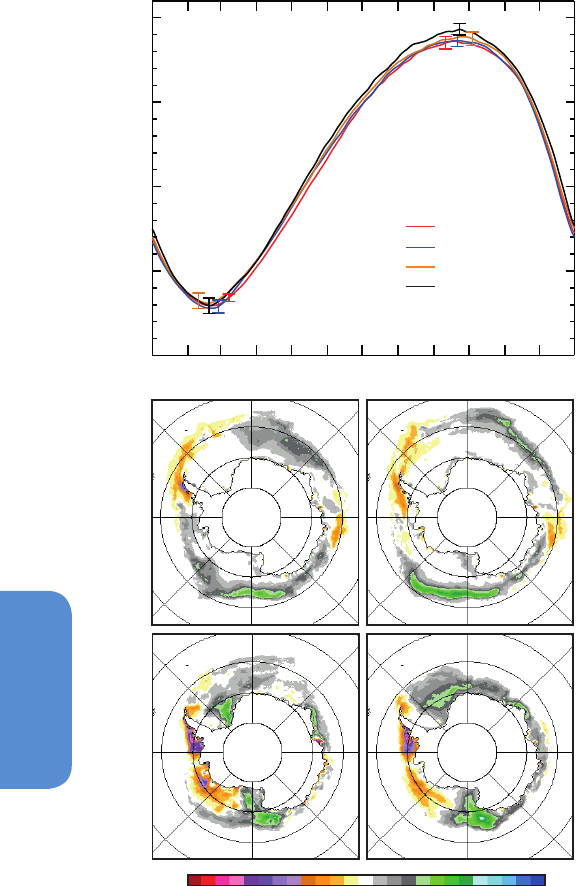
332

Chapter 4 Observations: Cryosphere

Figure 4.7 | (a) Plots of decadal averages of daily sea ice extent in the Antarctic

(1979–1988 in red, 1989–1998 in blue, 1999– 2008 in gold) and a 4-year average

daily ice extent from 2009 to 2012 in black. Maps indicate ice concentration trends

(1979–2012) in (b) winter, (c) spring, (d) summer and (e) autumn (updated from

Comiso, 2010).

a) Daily ice extent

JFMAMJJASOND

Ice extent (10

)

1979-1988

1989-1998

1999-2008

2009-2012

b) Winter (JJA) c) Spring (SON)

d) Summer (DJF)e) Autumn (MAM)

135

-2.4 -1.6 -0.8 0.0 0.8 1.6 2.4

Trend (% IC yr

-1

)

which routine observations of sea ice and snow properties were made.

Their compilation included a gridded data set that reﬂects the regional

differences in sea ice thickness. A subset of these ship observations,

and ice charts, was used by DeLiberty et al. (2011) to estimate the

annual cycle of sea ice thickness and volume in the Ross Sea, and to

investigate the relationship between ice thickness and extent. They

found that maximum sea ice volume was reached later than maxi-

mum extent. While ice is advected to the northern edge and melts, the

interior of the sea ice zone is supplied with ice from higher latitudes

and continues to thicken by thermodynamic growth and deformation.

Satellite retrievals of sea ice freeboard and thickness in the Antarctic

(Mahoney et al., 2007; Zwally et al., 2008; Xie et al., 2011) are under

development but progress is limited by knowledge of snow thickness

and the paucity of suitable validation data sets. A recent analysis of the

ICESat record by Kurtz and Markus (2012), assuming zero ice freeboard,

found negligible trends in ice thickness over the 5-year record.

4.2.3.3 Antarctic Sea Ice Drift

Using a 19-year data set (1992–2010) of satellite-tracked sea ice

motion, Holland and Kwok (2012) found large and statistically sig-

niﬁcant decadal trends in Antarctic ice drift that in most sectors are

caused by changes in local winds. These trends suggest acceleration of

the wind-driven Ross Gyre and deceleration of the Weddell Gyre. The

changes in meridional ice transport affect the freshwater budget near

the Antarctic coast. This is consistent with the increase of 30,000 km

–1

in the net area export of sea ice from the Ross Sea shelf coastal

polynya region between 1992 and 2008 (Comiso et al., 2011). Assum-

ing an annual average thickness of 0.6 m, Comiso et al. (2011) estimat-

ed an increase in volume export of 20 km

–1

which is similar to the

rate of production in the Ross Sea coastal polynya region for the same

period discussed in Section 4.2.3.5.

4.2.3.4 Timing of Sea Ice Advance, Retreat and Ice Season

Duration

In the Antarctic there are regionally different patterns of strong change

in ice duration (>2 days yr

–1

). In the northeast and west Antarctic

Peninsula and southern Bellingshausen Sea region, later ice advance

(+61 ± 15 days), earlier retreat (–39 ± 13 days) and shorter duration

(+100 ± 31 days,

a trend of –3.1

1.0 days

–1

)

occurred over

the period 1979/1980–

2010/2011

(Stammerjohn et al., 2012). These

changes have

strong impacts on the marine

ecosystem (Montes-

Hugo et al., 2009; Ducklow et al., 2011). The opposite is true in the

adjacent western Ross Sea, where substantial lengthening of the

ice season of 79 ± 12 days has occurred (+2.5 ± 0.4 days yr

–1

) due

to earlier advance (+42 ± 8 days) and later retreat (–37 ± 8 days).

Patterns of change in the relatively narrow East Antarctic sector are

generally of a lower magnitude and zonally complex, but in certain

regions involve changes in the timing of sea ice advance and retreat

of the order of ±1 to 2 days yr

–1

(for the period 1979–2009) (Massom

et al., 2013).

4.2.3.5 Antarctic Polynyas

Polynyas are commonly found along the coast of Antarctica. There are

two different processes that cause a polynya. Warm water upwelling

keeps the surface water near the freezing point and reduces ice pro-

duction (sensible heat polynya), and wind or ocean currents move ice

away and increase further ice production (latent heat polynya).

An increase in the extent of coastal polynyas in the Ross Sea caused

increased ice production (latent heat effect) that is primarily respon-

sible for the positive trend in ice extent in the Antarctic (Comiso et

al., 2011). Drucker et al. (2011) show that in the Ross Sea, the net

ice export equals the annual ice production in the Ross Sea polynya

(approximately 400 km

in 1992), and that ice production increased by

20 km

–1

from 1992 to 2008. However, the ice production in the Wed-

dell Sea, which is three times less, has had no statistically signiﬁcant

333

Observations: Cryosphere Chapter 4

Frequently Asked Questions

FAQ 4.1 | How Is Sea Ice Changing in the Arctic and Antarctic?

The sea ice covers on the Arctic Ocean and on the Southern Ocean around Antarctica have quite different charac-

teristics, and are showing different changes with time. Over the past 34 years (1979–2012), there has been a down-

ward trend of 3.8% per decade in the annual average extent of sea ice in the Arctic. The average winter thickness

of Arctic Ocean sea ice has thinned by approximately 1.8 m between 1978 and 2008, and the total volume (mass)

of Arctic sea ice has decreased at all times of year. The more rapid decrease in the extent of sea ice at the summer

minimum is a consequence of these trends. In contrast, over the same 34-year period, the total extent of Antarctic

sea ice shows a small increase of 1.5% per decade, but there are strong regional differences in the changes around

the Antarctic. Measurements of Antarctic sea ice thickness are too few to be able to judge whether its total volume

(mass) is decreasing, steady, or increasing.

A large part of the total Arctic sea ice cover lies above 60°N (FAQ 4.1, Figure 1) and is surrounded by land to the

south with openings to the Canadian Arctic Archipelago, and the Bering, Barents and Greenland seas. Some of the

ice within the Arctic Basin survives for several seasons, growing in thickness by freezing of seawater at the base and

by deformation (ridging and rafting). Seasonal sea ice grows to only ~2 m in thickness but sea ice that is more than

1 year old (perennial ice) can be several metres thicker. Arctic sea ice drifts within the basin, driven by wind and

ocean currents: the mean drift pattern is dominated by a clockwise circulation pattern in the western Arctic and a

Transpolar Drift Stream that transports Siberian sea ice across the Arctic and exports it from the basin through the

Fram Strait.

Satellites with the capability to distinguish ice and open water have provided a picture of the sea ice cover changes.

Since 1979, the annual average extent of ice in the Arctic has decreased by 3.8% per decade. The decline in extent

at the end of summer (in late September) has been even greater at 11% per decade, reaching a record minimum in

2012. The decadal average extent of the September minimum Arctic ice cover has decreased for each decade since

satellite records began. Submarine and satellite records suggest that the thickness of Arctic ice, and hence the total

volume, is also decreasing. Changes in the relative amounts of perennial and seasonal ice are contributing to the

reduction in ice volume. Over the 34-year record, approximately 17% of this type of sea ice per decade has been lost

to melt and export out of the basin since 1979 and 40% since 1999. Although the area of Arctic sea ice coverage can

ﬂuctuate from year to year because of variable seasonal production, the proportion of thick perennial ice, and the

total sea ice volume, can recover only slowly.

Unlike the Arctic, the sea ice cover around Antarctica is constrained to latitudes north of 78°S because of the pres-

ence of the continental land mass. The Antarctic sea ice cover is largely seasonal, with an average thickness of

only ~1 m at the time of maximum extent in September. Only a small fraction of the ice cover survives the summer

minimum in February, and very little Antarctic sea ice is more than 2 years old. The ice edge is exposed to the open

ocean and the snowfall rate over Antarctic sea ice is higher than in the Arctic. When the snow load from snowfall is

sufﬁcient to depress the ice surface below sea level, seawater inﬁltrates the base of the snow pack and snow-ice is

formed when the resultant slush freezes. Consequently, snow-to-ice conversion (as well as basal freezing as in the

Arctic) contributes to the seasonal growth in ice thickness and total ice volume in the Antarctic. Snow-ice forma-

tion is sensitive to changes in precipitation and thus changes in regional climate. The consequence of changes in

precipitation on Antarctic sea ice thickness and volume remains a focus for research.

Unconstrained by land boundaries, the latitudinal extent of the Antarctic sea ice cover is highly variable. Near the

Antarctic coast, sea ice drift is predominantly from east to west, but further north, it is from west to east and highly

divergent. Distinct clockwise circulation patterns that transport ice northward can be found in the Weddell and

Ross seas, while the circulation is more variable around East Antarctica. The northward extent of the sea ice cover is

controlled in part by the divergent drift that is conducive in winter months to new ice formation in persistent open

water areas (polynyas) along the coastlines. These zones of ice formation result in saltier and thus denser ocean

water and become one of the primary sources of the deepest water found in the global oceans.

Over the same 34-year satellite record, the annual extent of sea ice in the Antarctic increased at about 1.5% per

decade. However, there are regional differences in trends, with decreases seen in the Bellingshausen and Amundsen

seas, but a larger increase in sea ice extent in the Ross Sea that dominates the overall trend. Whether the smaller

overall increase in Antarctic sea ice extent is meaningful as an indicator of climate is uncertain because the extent

(continued on next page)

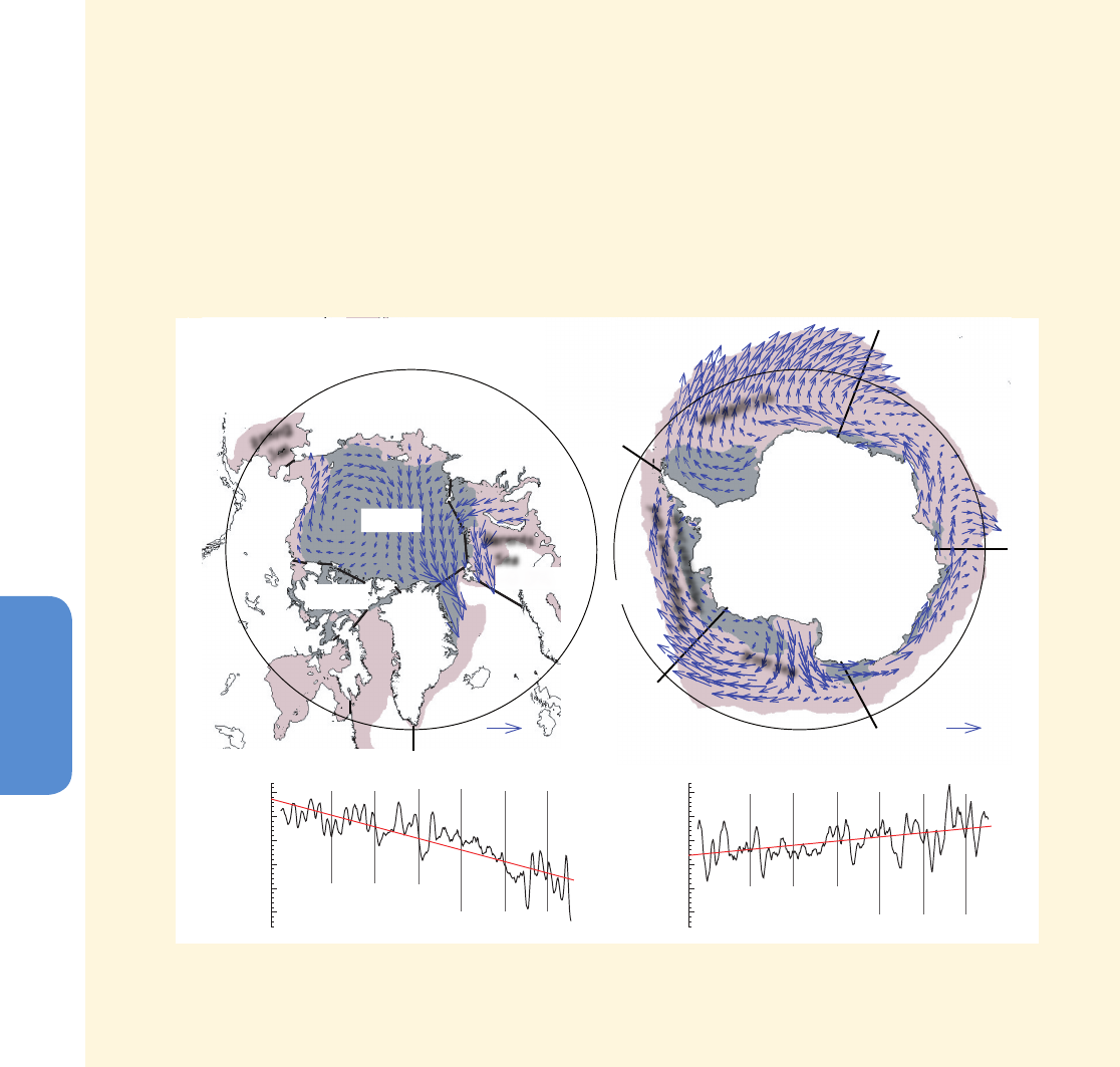
334

Chapter 4 Observations: Cryosphere

FAQ 4.1 (continued)

varies so much from year to year and from place to place around the continent. Results from a recent study suggest

that these contrasting trends in ice coverage may be due to trends in regional wind speed and patterns. Without

better ice thickness and ice volume estimates, it is difﬁcult to characterize how Antarctic sea ice cover is responding

to changing climate, or which climate parameters are most inﬂuential.

There are large differences in the physical environment and processes that affect the state of Arctic and Antarctic

sea ice cover and contribute to their dissimilar responses to climate change. The long, and unbroken, record of

satellite observations have provided a clear picture of the decline of the Arctic sea ice cover, but available evidence

precludes us from making robust statements about overall changes in Antarctic sea ice and their causes.

+1.3%

+3.2%

+1.3%

+4.3%

AntarcticArctic

10 km per day

60°S

Antarctica

1990 20102000

1.0

0.0

–1.0

Extent anomalies

(10

)

+1.5% per decade

–6.1%

5 km per day

–4.3%

Ross Sea

Weddell Sea

Bellingshausen and

Amundsen Seas

Barents

Sea

1990 20102000

+7.3%

–2.2%

60°N

Greenland

Alaska

Bering

Sea

-3.8% per decade

–7.0%

–4.6%

Siberia

1.0

0.0

–1.0

Extent anomalies

(10

)

–2.5%

–9.3%

FAQ 4.1, Figure 1 | The mean circulation pattern of sea ice and the decadal trends (%) in annual anomalies in ice extent (i.e., after removal of the seasonal

cycle), in different sectors of the Arctic and Antarctic. Arrows show the average direction and magnitude of ice drift. The average sea ice cover for the period

1979 through 2012, from satellite observations, at maximum (minimum) extent is shown as orange (grey) shading.

trend over the same period. Variability in the ice cover in this region

is linked to changes in the Southern Annular Mode (SAM). Between

1974 and 1976, the large Weddell Sea Polynya, which is a sensible heat

polynya, was created by the injection of relatively warm deep water

into the surface layer due to sustained deep-ocean convection (sensi-

ble heat effect) during negative SAM, but since the late 1970s the SAM

has been mainly positive, resulting in warmer and wetter condition

forestalling any reoccurrence of the Weddell Sea Polynya (Gordon et

al., 2007).

4.2.3.6 Antarctic Land-Fast Ice

Land-fast ice forms around the coast of Antarctica, typically in narrow

coastal bands of varying width up to 150 km from the coast and in

water depths of up to 400 to 500 m. Around East Antarctica, it com-

prises generally between 5% (winter) and 35% (summer) of the overall

sea ice area (Fraser et al., 2012), and a greater fraction of ice volume

(Giles et al., 2008a).

Variability in the distribution and extent of land-fast ice is sensitive to

processes of ice formation and to processes such as ocean swell and

335

Observations: Cryosphere Chapter 4

waves, and strong wind events that cause the ice to break-up. Histor-

ical records of Antarctic land-fast ice extent, such as that of Kozlovsky

et al. (1977) covering 0° to 160°E, were limited by sparse and sporad-

ic sampling. Recently, using cloud-free Moderate Resolution Imaging

Spectrometer (MODIS) composite images, Fraser et al. (2012) derived

a high-resolution time series of land-fast sea ice extent along the

East Antarctic coast, showing a statistically signiﬁcant increase (1.43

± 0.30% yr

–1

) between March 2000 and December 2008. There is a

strong increase in the Indian Ocean sector (20°E to 90°E, 4.07 ± 0.42%

–1

), and a non-signiﬁcant decrease in the sector from 90°E to 160°E

(–0.40 ± 0.37% yr

–1

). An apparent shift from a negative to a positive

trend was noted in the Indian Ocean sector from 2004, which coincid-

ed with greater interannual variability. Although signiﬁcant changes

are observed, this record is only 9 years in length.

4.2.3.7 Decadal Trends in Antarctic Sea Ice

For the Antarctic, any changes in many sea ice characteristics are

unknown. There has been a small but signiﬁcant increase in total annual

mean sea ice extent that is very likely in the range of 1.2 to 1.8 % per

decade between 1979 and 2012 (0.13 to 0.20 million km

per decade)

(very high conﬁdence). There was also a greater increase in ice area

associated with an increase in ice concentration. But there are strong

regional differences within this total, with some regions increasing in

extent/area and some decreasing (high conﬁdence). Similarly, there are

contrasting regions around the Antarctic where the ice-free season has

lengthened, and others where it has decreased over the satellite period

(high conﬁdence). There are still inadequate data to make any assess-

ment of changes to Antarctic sea ice thickness and volume.

4.3 Glaciers

This section considers all perennial surface land ice masses (deﬁned in

4.1 and Glossary) outside of the Antarctic and Greenland ice sheets.

Glaciers occur where climate conditions and topographic characteristics

allow snow to accumulate over several years and to transform grad-

ually into ﬁrn (snow that persists for at least one year) and ﬁnally to

ice. Under the force of gravity, this ice ﬂows downwards to elevations

with higher temperatures where various processes of ablation (loss of

snow and ice) dominate over accumulation (gain of snow and ice). The

sum of all accumulation and ablation processes determines the mass

balance of a glacier. Accumulation is in most regions due mainly to

solid precipitation (in general snow), but also results from refreezing

of liquid water, especially in polar regions or at high altitudes where

ﬁrn remains below melting temperature. Ablation is, in most regions,

mainly due to surface melting with subsequent runoff, but loss of ice

by calving (on land or in water; see Glossary) or sublimation (important

in dry regions) can also dominate. Re-distribution of snow by wind

and avalanches can contribute to both accumulation and ablation. The

energy and mass ﬂuxes governing the surface mass balance are direct-

ly linked to atmospheric conditions and are modiﬁed by topography

(e.g., due to shading). Glaciers are sensitive climate indicators because

they adjust their size in response to changes in climate (e.g., tempera-

ture and precipitation) (FAQ 4.2). Glaciers are also important season-

al to long-term hydrologic reservoirs (WGII, Chapter 3) on a regional

scale and a major contributor to sea level rise on a global scale (see

Section 4.3.3.4 and Chapter 13). In the following, we report global

glacier coverage (Section 4.3.1), how changes in length, area, volume

and mass are determined (Section 4.3.2) and the observed changes in

these parameters through time (Section 4.3.3).

4.3.1 Current Area and Volume of Glaciers

The total area covered by glaciers was only roughly known in AR4,

resulting in large uncertainties for all related calculations (e.g., overall

glacier volume or mass changes). Since AR4, the world glacier invento-

ry (WGMS, 1989) was gradually extended by Cogley (2009a) and Radić

and Hock (2010); and for AR5, a new globally complete data set of gla-

cier outlines (Randolph Glacier Inventory (RGI)) was compiled from a

wide range of data sources from the 1950s to 2010 with varying levels

of detail and quality (Arendt et al., 2012). Regional glacier-covered

areas for 19 regions were extracted from the RGI and supplemented

with the percentage of the area covered by glaciers terminating in tide-

water (Figure 4.8 and Table 4.2). The areas covered by glaciers that are

in contact with freshwater lakes are only locally available. The separa-

tion of so-called peripheral glaciers from the ice sheets in Greenland

and Antarctica is not easy. A new detailed inventory of the glaciers in

Greenland (Rastner et al., 2012) allows for estimation of their area,

volume, and mass balance separately from those of the ice sheet. This

separation is still incomplete for Antarctica, and values discussed here

(Figures 4.1, 4.8 to 4.11, Tables 4.2 and 4.4) refer to the glaciers on

the islands in the Antarctic and Sub-Antarctic (Bliss et al., 2013) but

exclude glaciers on the mainland of Antarctica that are separate from

the ice sheet. Regionally variable accuracy of the glacier outlines leads

to poorly quantiﬁed uncertainties. These uncertainties, along with

the regional variation in the minimum size of glaciers included in the

inventory, and the subdivision of contiguous ice masses, also makes

the total number of glaciers uncertain; the current best estimate is

around 170,000 covering a total area of about 730,000 km

. When

summed up, nearly 80% of the glacier area found in regions Antarctic

and Subantarctic (region 19), Canadian Arctic (regions 3 and 4), High

Mountain Asia (regions 13, 14 and 15), Alaska (region 5), and Green-

land (region 17) (Table 4.2).

From the glacier areas in the new inventory, total glacier volumes

and masses have been determined by applying both simple scaling

relations and ice-dynamical considerations (Table 4.2, and references

therein), however, both methods are calibrated with only a few hun-

dred glacier thickness measurements. This small sample means that

uncertainties are large and difﬁcult to quantify. The range of values as

derived from four global-scale studies for each of the 19 RGI regions

is given in Table 4.2, suggesting a global glacier mass that is likely

between 114,000 and 192,000 Gt (314 to 529 mm SLE). The numbers

and areas of glaciers reported in Table 4.2 are directly taken from RGI

2.0 (Arendt et al., 2012), with updates for the Low Latitudes (region 16)

and the Southern Andes (region 17).

4.3.2 Methods to Measure Changes in Glacier Length,

Area and Volume/Mass

To measure changes in glacier length, area, mass and volume, a wide

range of observational techniques has been developed. Each technique

has individual beneﬁts over speciﬁc spatial and temporal scales; their

336

Chapter 4 Observations: Cryosphere

Region Region Name

Number of

Glaciers

Area

( km

)

Percent of

total area

Tidewater

fraction (%)

Mass

(minimum)

(Gt)

Mass

(maximum)

(Gt)

Mean SLE

(mm)

1 Alaska 23,112 89,267 12.3 13.7 16,168 28,021 54.7

Western Canada

and USA

15,073 14,503.5 2.0 0 906 1148 2.8

3 Arctic Canada North 3318 103,990.2 14.3 46.5 22,366 37,555 84.2

4 Arctic Canada South 7342 40,600.7 5.6 7.3 5510 8845 19.4

5 Greenland 13,880 87,125.9 12.0 34.9 10,005 17,146 38.9

6 Iceland 290 10,988.6 1.5 0 2390 4640 9.8

7 Svalbard 1615 33,672.9 4.6 43.8 4821 8700 19.1

8 Scandinavia 1799 2833.7 0.4 0 182 290 0.6

9 Russian Arctic 331 51,160.5 7.0 64.7 11,016 21,315 41.2

10 North Asia

4403 3425.6 0.4 0 109 247 0.5

11 Central Europe 3920 2058.1 0.3 0 109 125 0.3

12 Caucasus 1339 1125.6 0.2 0 61 72 0.2

13 Central Asia 30,200 64,497 8.9 0 4531 8591 16.7

14 South Asia (West) 22,822 33,862 4.7 0 2900 3444 9.1

15 South Asia (East) 14,006 21,803.2 3.0 0 1196 1623 3.9

16 Low Latitudes

2601 2554.7 0.6 0 109 218 0.5

17 Southern Andes

15,994 29,361.2 4.5 23.8 4241 6018 13.5

18 New Zealand 3012 1160.5 0.2 0 71 109 0.2

Antarctic and

Sub-Antarctic

3274 13,2267.4 18.2 97.8 27,224 43,772 96.3

Total 168,331 726,258.3 38.5 113,915 191,879 412.0

Table 4.2 | The 19 regions used throughout this chapter and their respective glacier numbers and area (absolute and in percent) are derived from the RGI 2.0 (Arendt et al., 2012);

the tidewater fraction is from Gardner et al. (2013). The minimum and maximum values of glacier mass are the minimum and maximum of the estimates given in four studies:

Grinsted (2013), Huss and Farinotti (2012), Marzeion et al. (2012) and Radić et al. (2013). The mean sea level equivalent (SLE) of the mean glacier mass is the mean of estimates

from the same four studies, using an ocean area of 362.5 × 10

for conversion. All values were derived with globally consistent methods; deviations from more precise national

data sets are thus possible. Ongoing improvements may lead to revisions of these (RGI 2.0) numbers in future releases of the RGI.

Notes:

For regions 10, 16 and 17 the number and area of glaciers are corrected to allow for over-inclusion of seasonal snow in the glacierized extent of RGI 2.0 and for improved outlines (region 10)

compared to RGI 2.0 (updated from, Arendt et al., 2012).

main characteristics are summarized in Table 4.3. Monitoring programs

include complex climate-related observations at a few glaciers, index

measurements of mass balance at about a hundred glaciers, annual

length changes for a few hundred glaciers, and repeat geodetic esti-

mates of area and volume changes at regional scales using remote

sensing methods (e.g., Haeberli et al., 2007). Although in situ meas-

urements of glacier changes are biased towards glaciers that are easily

accessible, comparatively small and simple to interpret, a large propor-

tion of all glaciers in the world is debris covered or tidewater calving

(see Table 4.2) and changes of such glaciers are more difﬁcult to inter-

pret in climatic terms (Yde and Pasche, 2010). In addition, many of the

remote-sensing based assessments do not discriminate these types.

4.3.2.1 Length Change Measurements

For the approximately 500 glaciers worldwide that are regularly

observed, front variations (commonly called length changes) are usu-

ally obtained through annual measurements of the glacier terminus

position. Globally coordinated observations were started in 1894,

providing one of the longest available time series of environmental

change (WGMS, 2008). More recently, particularly in regions that are

difﬁcult to access, aerial photography and satellite imaging have been

used to determine glacier length changes over the past decades. For

selected glaciers globally, historic terminus positions have been recon-

structed from maps, photographs, satellite imagery, also paintings,

dated moraines and other sources (e.g., Masiokas et al., 2009; Lopez et

al., 2010; Nussbaumer et al., 2011; Davies and Glasser, 2012; Leclercq

and Oerlemans, 2012; Rabatel et al., 2013). Early reconstructions are

sparsely distributed in both space and time, generally at intervals of

decades. The terminus ﬂuctuations of some individual glaciers have

been reconstructed for periods of more than 3000 years (Holzhauser

et al., 2005), with a much larger number of records available as far

back as the 16th or 17th centuries (Zemp et al., 2011, and references

therein). The reconstructed glacier length records are globally well dis-

tributed and were used, for example, to determine the contribution of

glaciers to global sea level rise (Leclercq et al., 2011) (Section 4.3.3.4),

and for an independent temperature reconstruction at a hemispheric

scale (Leclercq and Oerlemans, 2012).

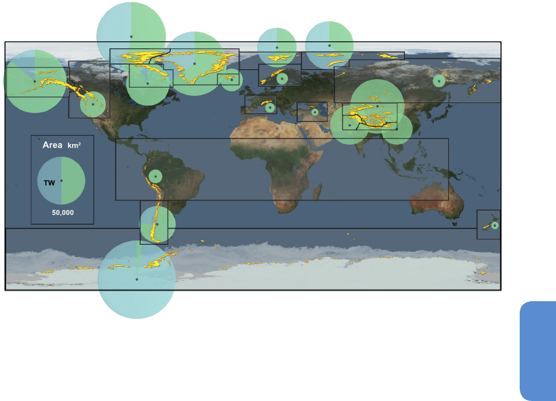
337

Observations: Cryosphere Chapter 4

Figure 4.8 | Global distribution of glaciers (yellow, area increased for visibility) and area covered (diameter of the circle), sub-divided into the 19 RGI regions (white number)

referenced in Table 4.2. The area percentage covered by tidewater (TW) glaciers in each region is shown in blue. Data from Arendt et al. (2012) and Gardner et al. (2013).

(

()

4.3.2.2 Area Change Measurements

Glacier area changes are reported in increasing number and cover-

age based on repeat satellite imagery (WGMS, 2008). Although satel-

lite-based observations are available only for the past four decades,

studies using aerial photography, old maps, as well as mapped and

dated moraines and trim lines show glacier areas back to the end of

the so-called Little Ice Age (LIA, see Glossary) about 150 years ago (cf.

Figure 6 in Rabatel et al., 2008) and beyond (e.g., Citterio et al., 2009;

Davies and Glasser, 2012). The observed area changes depend (in

most regions) on glacier size (with smaller glaciers shrinking at faster

percentage rates) and tend to vary greatly within any one mountain

range. Moreover, the time spans of the measurements of change vary

from study to study and regional or global-scale estimates are there-

fore difﬁcult to generate. The focus here is thus on the comparison of

mean annual relative area changes averaged over entire mountain

regions.

4.3.2.3 Volume and Mass Change Measurements

Several methods are in use for measuring mass changes of glaciers.

Traditionally, the annual surface mass balance is derived from repeated

snow density and snow/ice stake readings on individual glaciers. Esti-

mates over larger regions are obtained by extrapolating from the mea-

sured glaciers. This labour-intensive method is generally restricted to a

limited number of accessible glaciers, which are unevenly distributed

over glacier regions and types. Annual measurements began in the

1940s on a few glaciers, with about 100 glaciers being measured since

the 1980s—and only 37 glaciers have been measured without inter-

ruption for more than 40 years (WGMS, 2009). Potential mass loss from

calving or from basal ablation is not included in the surface measure-

ments. At present, it is not possible to quantify all sources of uncer-

tainty in mass budgets extrapolated from measurements of individual

glaciers (Cogley, 2009b).

A second method determines the volume change of all glaciers in a

region by measurement of surface-elevation changes (Section 4.3.3.3

and Figure 4.11). The information is derived by subtracting digital ter-

rain models from two points in time, including those from repeat air-

borne or satellite altimetry (particularly suitable for larger and ﬂatter

ice surfaces). The conversion from volume to mass change can cause

a major uncertainty, in particular over short periods, as density infor-

mation is required, but is generally available only from ﬁeld measure-

ments (Gardner et al., 2013, and references therein).

Since 2003, a third method used to estimate overall mass change is

through measurement of the changing gravity ﬁeld from satellites

(GRACE mission). The coarse spatial resolution (about 300 km) and the

difﬁculties of separating different mass change signals such as hydro-

logical storage and glacial isostatic adjustment limit this method to

regions with large continuous ice extent (Gardner et al., 2013).

338

Chapter 4 Observations: Cryosphere

A fourth method calculates the mass balance of individual glaciers,

or a glacier region, with models that either convert particular glacier

variables such as length changes or the altitude of the equilibrium line

(see Glossary) (e.g., Rabatel et al., 2005; Luethi et al., 2010; Leclercq

et al., 2011) into mass changes, or use time series of atmospheric tem-

perature and other meteorological variables to simulate glacier mass

balances at different levels of complexity (e.g., Hock et al., 2009; Mach-

guth et al., 2009; Marzeion et al., 2012; Hirabayashi et al., 2013). The

models improve ﬁdelity and physical completeness, and add value to

the scarce direct measurements.

A ﬁfth method determines glacier mass changes as residuals of the

water balance for hydrological basins rather than for glacier regions.

Results from all but this last method are used in the following regional

and global assessment of glacier mass changes (Sections 4.3.3.3 and

4.3.3.4).

4.3.3 Observed Changes in Glacier Length, Area and Mass

4.3.3.1 Length Changes

Despite their variability due to different response times and local con-

ditions (see FAQ 4.2), the annually measured glacier terminus ﬂuctu-

ations from about 500 glaciers worldwide reveal a largely homoge-

neous trend of retreat (WGMS, 2008). In Figure 4.9, a selection of the

available long-term records of ﬁeld measurements is shown for 14 out

of the 19 RGI regions. Cumulative values of retreat for large, land-ter-

minating valley glaciers typically reach a few kilometres over the 120-

year period of observation. For mid-latitude mountain and valley gla-

ciers, typical retreat rates are of the order of 5 to 20 m yr

–1

. Rates of up

to 100 m yr

–1

(or even more) are seen to occur under special conditions,

such as the complete loss of a tongue on a steep slope (see FAQ 4.2,

Figure 1c), or the disintegration of a very ﬂat tongue. A non-calving

valley glacier in Chile had reported mean annual retreat rates of 125 m

from 1961 to 2011 (Rivera et al., 2012). The general tendency of retreat

in the 20th century was interrupted in several regions (e.g., regions

2, 8, 11 and 17) by phases of stability lasting one or two decades, or

even advance, for example in the 1920s, 1970s and 1990s (regionally

variable). In regions for which long-term ﬁeld measurements of sev-

eral glaciers of different sizes are available, the terminus ﬂuctuations

Parameter Method Technique Typical Accuracy

Number of

Glaciers

Repeat

Interval

Earliest Data

Length change

Various Reconstruction 10 m Dozens

Decadal –

centuries

Holocene

Field In situ measurement 1 m Hundreds Annual 19th century

Remote sensing Photogrammetric survey Two image pixels (depending on resolution) Hundreds Annual 20th century

Area change

Maps Cartographic 5% of the area Hundreds Decadal 19th century

Remote sensing Image processing 5% of the area Thousands Sub-decadal 20th century

Volume change

Remote sensing Laser and radar proﬁling 0.1 m Hundreds Annual 21st century

Remote sensing DEM differencing 0.5 m Thousands Decadal 20th century

Mass change

Field Direct mass balance measurement 0.2 m Hundreds Seasonal 20th century

Remote sensing Gravimetry (GRACE) Dependent on the region Global Seasonal 21st century

Table 4.3 | Overview of methods used to determine changes in glacier length, area and volume mass along with some typical characteristics. The techniques are not exclusive.

The last three columns provide only indicative values.

typically show a pattern with the largest (ﬂatter) glaciers tending to

retreat continuously and by large cumulative distances, medium-sized

(steeper) glaciers showing decadal ﬂuctuations, and smaller glaciers

showing high variability superimposed on smaller cumulative retreats

(Figure 4.9).

The exceptional terminus advances of a few individual glaciers in Scan-

dinavia and New Zealand in the 1990s may be related to locally spe-

ciﬁc climatic conditions such as increased winter precipitation (Nesje

et al., 2000; Chinn et al., 2005; Lemke et al., 2007). In other regions,

such as Iceland, the Karakoram and Svalbard, observed advances

were often related to dynamical instabilities (surging) of glaciers (e.g.,

Murray et al., 2003; Quincey et al., 2011; Bolch et al., 2012; Björnsson

et al., 2013). Glaciers with calving instabilities can retreat exceptionally

rapidly (Pfeffer, 2007), while those with heavily debris-covered tongues

are often close to stationary (Scherler et al., 2011). More regionally-

focused studies of length change over different time periods (e.g., Cit-

terio et al., 2009; Masiokas et al., 2009; Lopez et al., 2010; Bolch et al.,

2012) justify high conﬁdence about the trend of glacier length varia-

tions shown in Figure 4.9.

4.3.3.2 Area Changes

From the large number of published studies on glacier area changes

in all parts of the world since AR4 (see Table 4.SM.1) a selection with

examples from 16 out of the 19 RGI regions is shown in Figure 4.10. The

studies reveal that (1) total glacier area has decreased in all regions,

(2) the rates of change cover a similar range of values in all regions,

(3) there is considerable variability of the rates of change within each

region, (4) highest loss rates are found in regions 2, 11 and 16, and (5)

the rates of loss have a tendency to be higher over more recent time

periods. The last point (5) requires studies comparing the same sample

of glaciers over multiple similar time periods. For 14 out of 19 regions

listed in Table 4.SM.1 (see Supplementary Material) with such an anal-

ysis, higher loss rates were found for the more recent period.

While points (1) and (2) give high conﬁdence in the global-scale shrink-

age in glacier area, (3) points to a considerable regional to local-scale

scatter of observed change rates. The shorter the period of investiga-

tion and the smaller the sample of glaciers analysed, the more variable

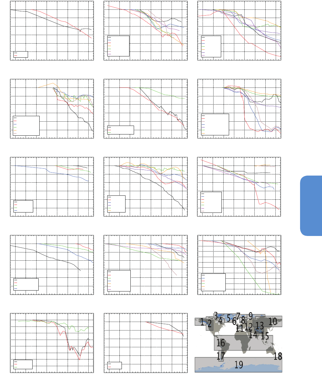
339

Observations: Cryosphere Chapter 4

1860 1880 1900 1920 1940 1960 1980 2000

-3000

-2500

-2000

-1500

-1000

-500

500

Cumulative length change (m)

Nuka

Okpilak

1860 1880 1900 1920 1940 1960 1980 2000

-3000

-2500

-2000

-1500

-1000

-500

500

Blue

Grifﬁn

Nisqually

Peyto

Sasketchewan

Sentinel

Wedgemount

1860 1880 1900 1920 1940 1960 1980 2000

-3000

-2500

-2000

-1500

-1000

-500

500

Sermikavsak

Sorqaup

Tunorssuaq

Sigssarigsut

Serminguaq

Motzfeld

Sermitsiaq

1860 1880 1900 1920 1940 1960 1980 2000

-3000

-2500

-2000

-1500

-1000

-500

500

Cumulative length change (m)

Breidamerkurjokull

Fjallsjokull G-Sel

Gljufurarjokull

Mulajokull

Skeidararjokull E3

Solheimajokull

1860 1880 1900 1920 1940 1960 1980 2000

-3000

-2500

-2000

-1500

-1000

-500

500

Hansbreen

Nordenskioldbreen

Waldemarbreen

1860 1880 1900 1920 1940 1960 1980 2000

-3000

-2500

-2000

-1500

-1000

-500

500

Brikdalsbreen

Engabreen

Faabergstoelsbreen

Nigardsbreen

Storbreen

Storglaciaeren

Styggedalbreen

1860 1880 1900 1920 1940 1960 1980 2000

-3000

-2500

-2000

-1500

-1000

-500

500

Cumulative length change (m)

Kara-batkak

Kljuev

Korumdu

Koryto

1860 1880 1900 1920 1940 1960 1980 2000

-3000

-2500

-2000

-1500

-1000

-500

500

Gr.Aletsch

Hornkees

Lys

Pasterze

Pizol

Trient

1860 1880 1900 1920 1940 1960 1980 2000

-3000

-2500

-2000

-1500

-1000

-500

500

Abano

Bezengi

Bolshoy Azau

Devdoraki

Djankuat

Gergeti

Khakel

1860 1880 1900 1920 1940 1960 1980 2000

-3000

-2500

-2000

-1500

-1000

-500

500

Cumulative length change (m)

Geblera

Levi Aktru

Maliy Aktru

Ts.Tuyuksuyskiy

1860 1880 1900 1920 1940 1960 1980 2000

-3000

-2500

-2000

-1500

-1000

-500

500

Broggi

Chacaltaya

Charquini Norte

Lewis

Meren

Tyndall

Zongo

1860 1880 1900 1920 1940 1960 1980 2000

-5000

-4500

-4000

-3500

-3000

-2500

-2000

-1500

-1000

-500

500

Azufre

Esperanza Norte

Frias

Guessfeldt

Upsala

Vacas

1860 1880 1900 1920 1940 1960 1980 2000

-4000

-3500

-3000

-2500

-2000

-1500

-1000

-500

500

Cumulative length change (m)

Fox

Franz Josef

Stocking

1860 1880 1900 1920 1940 1960 1980 2000

-3000

-2500

-2000

-1500

-1000

-500

500

Heaney

Hodges

1Alaska 2 Western Canada and US 5 Greenland

8 Scandinavia

12 Caucasus and Middle East11 Central Europe

7 Svalbard6 Iceland

10 North Asia

13 Central Asia 16 Low Latitudes17 Southern Andes

18 New Zealand19 Antarctic and Subantarctic

Region overview

Figure 4.9 | Selection of long-term cumulative glacier length changes as compiled from in situ measurements (WGMS, 2008), reconstructed data points added to measured time

series (region 5) from Leclercq et al. (2012), and additional time series from reconstructions (regions 1, 2, 7, 10, 12, 16, 17 and 18) from Leclercq and Oerlemans (2012). Indepen-

dent of their (highly variable) temporal density, all measurement points are connected by straight lines. The glacier Mulajokull (region 6) is of surge type and some of the glaciers

showing strong retreat either terminate (Guessfeldt and Upsala in region 17) or terminated (Engabreen and Nigardsbreen in region 8) in lakes. For region 11, many more time series

are available (see WGMS, 2008), but are not shown for graphical reasons.

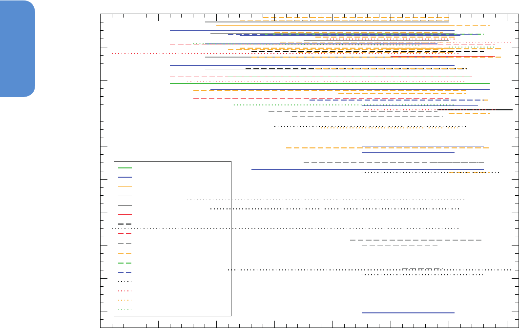
340

Chapter 4 Observations: Cryosphere

are the rates of change reported for a speciﬁc region (Table 4.SM.1).

In many regions of the world, rates of area loss have increased (Table

4.SM.1), conﬁrming that glaciers are still too large for the current cli-

mate and will continue to shrink (see FAQ 4.2 and Section 4.3.3.3).

Several studies have reported the disappearance of glaciers, among

others in Arctic Canada (Thomson et al., 2011), the Rocky Mountains

(Bolch et al., 2010; Tennant et al., 2012) and North Cascades (Pelto,

2006), Patagonia (Bown et al., 2008; Davies and Glasser, 2012), sever-

al tropical mountain ranges (Coudrain et al., 2005; Klein and Kincaid,

2006; Cullen et al., 2013), the European Alps (Citterio et al., 2007;

Knoll and Kerschner, 2009; Diolaiuti et al., 2012), the Tien Shan (Hagg

et al., 2012; Kutuzov and Shahgedanova, 2009) in Asia and on James

Ross Island in Antarctica (Carrivick et al., 2012). In total, the disap-

pearance of more than 600 glaciers has been reported, but the real

number is certainly higher. Also some of the glaciers, whose annual

mass balance has been measured over several years or even decades,

have disappeared or started to disintegrate (Ramirez et al., 2001; Car-

turan and Seppi, 2007; Thibert et al., 2008). Though the number of

glaciers that have disappeared is difﬁcult to compare directly (e.g., the

time periods analysed or the disappearance-criteria applied differ),

glaciers that have disappeared provide robust evidence that the ELA

(see Glossary) has risen above the highest peaks in many mountain

ranges (see FAQ 4.2).

1940 1950 1960 1970 1980 1990 2000 2010

-1.8

-1.6

-1.4

-1.2

-1

-0.8

-0.6

-0.4

-0.2

Relative area change rate (% yr

-1

)

Year

1 Alaska

2 Western Canada / US

3 Arctic Canada N

4 Arctic Canada S

6 Iceland

7 Svalbard

8 Scandinavia

10 North Asia

11 Central Europe

13 Central Asia

14 South Asia W

15 South Asia E

16 Low Latitudes

17 Southern Andes

18 New Zealand

19 Antarcic / Subantarctic

Figure 4.10 | Mean annual relative area loss rates for 16 out of the 19 RGI regions of Figure 4.8. Each line shows a measurement of the rate of percentage change in area over

a mountain range from a speciﬁc publication (for sources see Table 4.SM.1), the length of the line shows the period used for averaging.

4.3.3.3 Regional Scale Glacier Volume and Mass Changes

In AR4, global and regional scale glacier mass changes were extrapo-

lated from in situ measurements of mass balance on individual glaciers

(Kaser et al., 2006; Lemke et al., 2007). In some regions, such as Alaska,

Patagonia and the Russian Arctic, very few if any such records were

available. Since AR4, geodetically derived ice volume changes have

been assimilated (Cogley, 2009b), providing more consistent regional

coverage and better representation of the proportion of calving gla-

ciers. In addition, the new near complete inventory (RGI) of glacier-cov-

ered areas (Arendt et al., 2012) has improved knowledge about region-

al and global glacier volume and mass changes.

Figure 4.11 shows a compilation of available mean mass-balance rates

for 1960–2010 for each of the 19 RGI regions. Where error estimates

are reported, the 90% conﬁdence bounds are shown. Most results

shown are calculated using a single method, some merge multiple

methods; those from Gardner et al. (2013) are reconciled estimates

for 2003–2009 obtained by selecting the most reliable results of dif-

ferent observation methods, after region-by-region reanalysis and

comparison.

Despite the great progress made since AR4, uncertainties inherent to

speciﬁc methods, and arising from the differences between methods (cf.

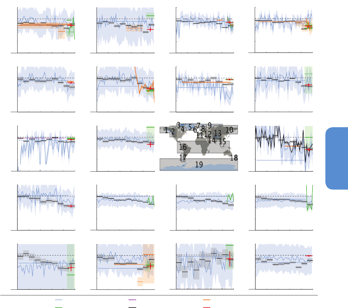
341

Observations: Cryosphere Chapter 4

Figure 4.11 | Regional glacier mass budgets in units of kg m

–2

–1

for the world’s 19 glacierized regions (Figure 4.8 and Table 4.2). Estimates are from modelling with climate data

(blue: Hock et al., 2009; Marzeion et al., 2012), repeat gravimetry (green: Chen et al., 2007; Luthcke et al., 2008; Peltier, 2009; Matsuo and Heki, 2010; Wu et al., 2010; Gardner

et al., 2011; Ivins et al., 2011; Schrama and Wouters, 2011; Jacob et al., 2012, updated for RGI regions), repeat volume area scaling (magenta: Glazovsky and Macheret, 2006),

interpolation of local glacier records (black: Cogley, 2009a; Huss, 2012), or airborne and/or satellite repeat topographic mapping (orange: Arendt et al., 2002; Rignot et al., 2003;

Abdalati et al., 2004; Schiefer et al., 2007; Paul and Haeberli, 2008; Berthier et al., 2010; Moholdt et al., 2010, 2012; Nuth et al., 2010; Gardner et al., 2011, 2012; Willis et al., 2012;

Björnsson et al., 2013; Bolch et al., 2013). Mass-budget estimates are included only for study domains that cover about 50% or more of the total regional glacier area. Mass-budget

estimates include 90% conﬁdence envelopes (not available from all studies). Conversions from speciﬁc mass budget in kg m

–2

to mm SLE are given for each region. Gravimetric

estimates are often not accompanied by estimates of glacierized area (required for conversion from Gt yr

–1

to kg m

–2

–1

); in such cases the RGI regional glacier areas were used.

960

980

990

000

−2000

−1000

1000

Alaska

960

980

990

000

−2000

−1000

1000

Western Canada/US

960

980

990

000

−2000

−1000

1000

Arctic Canada North

960

980

990

000

−2000

−1000

1000

Arctic Canada South

960

980

990

000

−2000

−1000

1000

Greenland

960

980

990

000

−2000

−1000

1000

Iceland

960

980

990

000

−2000

−1000

1000

Svalbard

960

980

990

000

−2000

−1000

1000

Scandinavia

960

980

990

000

−2000

−1000

1000

Russian Arctic

960

980

990

000

−2000

−1000

1000

North Asia

960

980

990

000

−2000

−1000

1000

Central Europe

960

980

990

000

−2000

−1000

1000

Caucasus & Middle East

960

980

990

000

−2000

−1000

1000

Central Asia

960

980

990

000

−2000

−1000

1000

South Asia (West)

960

980

990

000

−2000

−1000

1000

South Asia (East)

960

980

990

000

−2000

−1000

1000

Low Latitudes

960

980

990

000

−2000

−1000

1000

Southern Andes

960

980

990

000

−2000

−1000

1000

New Zealand

960

980

990

000

−2000

−1000

1000

Antarctic & Subantarctic

modeled with climate data

repeat gravimetry

repeat topography

interpolated local records

repeat volume area scaling

Gardner et al. 2013 [mixed]

-1000 kg m = 0.243 mm SLE -1000 kg m = 0.04 mm SLE -1000 kg m = 0.289 mm SLE -1000 kg m = 0.113 mm SLE

-1000 kg m = 0.248 mm SLE -1000 kg m = 0.031 mm SLE -1000 kg m = 0.094 mm SLE -1000 kg m = 0.008 mm SLE

-1000 kg m = 0.142 mm SLE -1000 kg m = 0.009 mm SLE -1000 kg m = 0.006 mm SLE

-1000 kg m = 0.003 mm SLE -1000 kg m = 0.178 mm SLE -1000 kg m = 0.093 mm SLE -1000 kg m = 0.06 mm SLE

-1000 kg m = 0.011 mm SLE -1000 kg m = 0.087 mm SLE -1000 kg m = 0.003 mm SLE -1000 kg m = 0.368 mm SLE

Mass budget (kg m yr)

Box 2.1), remain large, and conﬁdence about the absolute value of mass

loss is medium at both regional and global scales (Figure 4.11). The

highest density of measurement and best time resolution are available

for Scandinavia (region 8) and Central Europe (region 11). The least cov-

erage and some of the highest uncertainties are in the Arctic (regions 3,

4, 5, 9) and the Antarctic and Sub-Antarctic (region 19).

Gardner et al. (2013) discussed inconsistencies among, and differences

between, methods and their respective results for 2003–2009. They

found that results from the GRACE gravimetric mission agree well with

results from ICESat laser altimetry in regions of extensive ice cover (see

comment on ICESat data in Section 4.4.2.1), but show much more vari-

able and uncertain mass changes in regions with small or scattered ice

342

Chapter 4 Observations: Cryosphere

cover such as Western Canada/USA (region 2) and the Qinghai-Xizang

(Tibet) Plateau (e.g., Yao et al., 2012, and references therein). Based

on ICESat measurements, Gardner et al. (2013) also found that glaciers

with in situ measurements tend to be located in sub-regions that are

thinning more rapidly than the region as a whole. Thus, extrapolation

from in situ measurements has a negative bias in regions with sparse

measurements. Based on this analysis, Gardner et al. (2013) excluded

GRACE results for regions with small or scattered glacier coverage and

excluded results based on extrapolation of local records for remote,

sparsely sampled regions.

The 2003–2009 regionally differentiated results are given in Table 4.4.

There is very high conﬁdence that, between 2003 and 2009, most mass

loss was from glaciers in the Canadian Arctic (regions 3 and 4), Alaska

(region 1), Greenland (region 5), the Southern Andes (region 17) and

the Asian Mountains (region 13 to 15), which together account for

more than 80% of the global ice loss.

Despite the considerable scatter, Figure 4.11 shows mass losses in all

19 regions over the past ﬁve decades that, together with their consist-

ency with length (Section 4.3.3.1) and area changes (Section 4.3.3.2),

provide robust evidence and very high conﬁdence in global glacier

shrinkage. In many regions, ice loss has likely increased during the last

two decades, with slightly smaller losses in some regions during the

most recent years, since around 2005. In Central Europe (region 11),

the increase of loss rates was earliest and strongest. In the Russian

Arctic (region 9) and in the Antarctic and Sub-Antarctic (region 19),

the signal is highly uncertain and trends are least clear. Gardner et al.

(2013) present values close to balance for the Antarctic and Subant-

arctic (region 19) that result from complex regional patterns, for exam-

Table 4.4 | Regional mass change rates in units of kg m

–2

–1

and Gt y

r–1

for the

period 2003–2009 from Gardner et al. (2013). Central Asia (region 13), South Asia

West (region14), and South Asia East (region 15) are merged into a single region. For

the division of regions see Figure 4.8.

No. Region Name (kg m

–2

–1

) (Gt yr

–1

)

1 Alaska –570 ± 200 –50 ± 17

2 Western Canada and USA –930 ± 230 –14 ± 3

3 Arctic Canada North –310 ± 40 –33 ± 4

4 Arctic Canada South –660 ± 110 –27 ± 4

5 Greenland periphery –420 ± 70 –38 ± 7

6 Iceland –910 ± 150 –10 ± 2

7 Svalbard –130 ± 60 –5 ± 2

8 Scandinavia –610 ± 140 –2 ± 0

9 Russian Arctic –210 ± 80 –11 ± 4

10 North Asia –630 ± 310 –2 ± 1

11 Central Europe –1060 ± 170 –2 ± 0

12 Caucasus and Middle East –900 ± 160 –1 ± 0

13–15 High Mountain Asia –220 ± 100 –26 ± 12

16 Low Latitudes –1080 ± 360 –4 ± 1

17 Southern Andes –990 ± 360 –29 ± 10

18 New Zealand –320 ± 780 0 ± 1

19 Antarctic and Sub-Antarctic –50 ± 70 –6 ± 10

Total –350 ± 40 –259 ± 28

ple, with losses on Antarctic Peninsula islands and gains on Ellsworth

Land islands. The picture is also heterogeneous in High Mountain Asia

(region 13 to 15) (e.g., Bolch et al., 2012; Yao et al., 2012), where

glaciers in the Himalaya and the Hindu Kush have been losing mass

(Kääb et al., 2012) while those in the Karakoram are close to balance

(Gardelle et al., 2012).

Several studies of recent glacier velocity change (Heid and Kääb, 2012;

Azam et al., 2012) and of the worldwide present-day sizes of accu-

mulation areas (Bahr et al., 2009) indicate that the world’s glaciers

are out of balance with the present climate and thus committed to

losing considerable mass in the future, even without further changes in

climate. Increasing ice temperatures recorded at high elevation sites in

the tropical Andes (Gilbert et al., 2010) and in the European Alps (Col

du Dome on Mont Blanc and Monte Rosa) (Vincent et al., 2007; Hoelzle

et al., 2011), as well as the ongoing thinning of the cold surface layer

on Storglaciären in northern Sweden (Gusmeroli et al., 2012), support

this conclusion and give it high conﬁdence.

4.3.3.4 Global Scale Glacier Mass Changes—The

Contribution to Sea Level

Global time series are required to assess the continuing contribution

of glacier mass changes to sea level (see Section 13.4.2 for discus-

sion of the small proportion of ice loss from glaciers that does not

contribute to sea level rise). A series of recent studies, some updated

to RGI areas for this report by their respective authors, provides very

high conﬁdence in a considerable and continuous mass loss, despite

only medium agreement on the speciﬁc rates (Figure 4.12 and Table

4.5). Cogley (updated from, 2009b) compiled 4,817 directly meas-

ured annual mass budgets, and 983 volume change measurements by

extending the data set of WGMS (2009, and earlier issues ). Global

5-year averages for 1961–2010, with uncertainties, were estimated

from these using an inverse-distance-weighted interpolation. Newly

available volume change measurements increased the proportion of

observations from calving glaciers from 3% to 16% compared to ear-

lier estimates reported by Lemke et al. (2007). This proportion is more

realistic, but may still underestimate the relative importance of calving

glaciers (Figure 4.8 and Section 4.3.3.3).

Leclercq et al. (updated from 2011) used length variations from 382

glaciers worldwide as a proxy for glacier mass loss since 1800. The

length/mass change conversion was calibrated against mass bal-

ance observations for 1950–2005 from Cogley (2009b) and provide

one estimate based on the arithmetic mean and another based on

area-weighted extrapolation of regional averages. Uncertainty was

estimated from upper and lower bounds of the calibration parameter

assumptions, and cumulatively propagated backward in time. For the

19th century, the information was constrained by a limited number of

observations, particularly in extensively glacierized regions that con-

tribute most to the global mass budget.

Two global-scale time series are obtained from mass-balance mod-

elling based on temperature and precipitation data (Marzeion et al.,

2012; Hirabayashi et al., 2013). Glacier size adjustments are simulated

by using area–volume power-law relations as proposed by Bahr et al.

(1997) for the approximately 170,000 individual glaciers delineated in

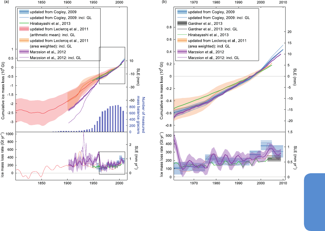
343

Observations: Cryosphere Chapter 4

the RGI. Marzeion et al. (2012) derive mass balances for 1902–2009

from monthly mean temperature and precipitation obtained from

Mitchell and Jones (2005). The model is calibrated against meas-

ured time series and validated against independent measurements.

Uncertainty estimates are obtained from comprehensive error propa-

gation, ﬁrst accumulated temporally for each glacier, and then region-

ally and globally. The model does not account for the subsurface mass

balance or calving, but reproduces geodetically measured volume

changes for land-based glaciers within the uncertainties; however, it

underestimates volume loss slightly for calving glaciers. Hirabayashi et

al. (2013) force an extended positive degree-day model with data from

an observation-based global set of daily precipitation and near-surface

temperature as updated from earlier work (Hirabayashi et al., 2008).

Annual mass balance is provided for 1948–2005 with a constant root

mean square error of 500 km

–1

, estimated from comparison of mod-

elled with measured mass balances.

For the Antarctic and Sub-Antarctic (region 19) observational infor-

mation is limited and difﬁcult to incorporate into this assessment.

For some studies the time spans do not match (e.g., Gardner et al.,

2013 give only mean mass change for 2003–2009). Some estimates

have been made simply by extrapolating the global mean to region

19 (Cogley, 2009a; Marzeion et al., 2012). One (1961–2004) mean

glacier mass loss estimate based on an ECMWF 40-year reanalysis

(ERA-40) driven simulation (Hock et al., 2009), is for a glacier area

differing from the RGI region 19. For these reasons, the Antarctic and

Sub-Antarctic (region 19) is excluded from this global glacier mass

change assessment. The contribution of region 19 to sea level is

assumed to be within the uncertainty bounds of the Antarctic ice sheet

assessment (Section 4.4.2). Whereas Hirabayashi et al. (2013) exclude

the Antarctic and Greenland from their simulations and Leclercq et al.

(2011) implicitly include Greenland, both Cogley (2009a) and Mar-

zeion et al. (2012) explicitly estimate mass changes in Greenland. In

Figure 4.12, cumulative mass changes and corresponding rates are

shown for global glaciers excluding regions 5 and 19 (bold lines),

and also for global glaciers excluding only region 19 (thin lines). The

cumulative curves are normalized such that their 1986–2005 aver-

ages are all zero.

The arithmetic-mean estimate of Leclercq et al. (2011) indicates con-

tinuous mass loss from glaciers after about 1850 (Figure 4.12a, top).

During the 1920s their area-weighted extrapolation reaches consid-

Figure 4.12 | Global cumulative (top graphs) and annual (lower graphs) glacier mass change for (a) 1801–2010 and (b) 1961–2010. The cumulative estimates are all set to

zero mean over 1986–2005. Estimates are based on glacier length variations (updated from Leclercq et al., 2011), from area-weighted extrapolations of individual directly and

geodetically measured glacier mass budgets (updated from Cogley, 2009b), and from modelling with atmospheric variables as input (Marzeion et al., 2012; Hirabayashi et al.,

2013). Uncertainties are based on comprehensive error analyses in Cogley (2009b) and Marzeion et al. (2012) and on assumptions about the representativeness of the sampled

glaciers in Leclercq et al. (2011). Hirabayashi et al. (2013) give a bulk error estimate only. For clarity in the bottom panels, uncertainties are shown only for the Cogley and Marzeion

curves excluding Greenland (GL). The blue bars (a, top) show the number of measured single-glacier mass balances per pentad in the updated Cogley (2009b) time series. The mean

2003–2009 estimate of Gardner et al. (2013) is added to b, bottom.

344

Chapter 4 Observations: Cryosphere

Table 4.5 | Average annual rates of global mass change in Gt yr

–1

and in sea level equivalents (mm SLE yr

–1

) for different time periods (Chapter 13) for (a) glaciers around the

Greenland ice sheet (region 5 as deﬁned by Rastner et al., 2012) and (b) all glaciers globally, excluding peripheral glaciers around the Antarctic and Greenland ice sheets (see dis-

cussion in Section 4.4.2). The values are derived by averaging the results from the references listed and uncertainty ranges give 90% conﬁdence level. The uncertainty calculated for

1971–2009 is also applied for the sub-periods 1993–2009 and 2005–2009. The global values for 2003–2009 from Gardner et al. (2013) are within this likelihood range (italics).

Reference

(a) Greenland glaciers (region 5) (b) All glaciers excluding ice sheet peripheries

Gt yr

–1

mm SLE yr

–1

Gt yr

–1

mm SLE yr

–1

1901–1990

Marzeion et al. (2012); Leclercq

et al. (2011), updated

–54 ± 16 0.15 ± 0.05 –197 ± 24 0.54 ± 0.07

1971–2009 Cogley (2009a); Marzeion et al. (2012) –21 ± 10 0.06 ± 0.03 –226 ± 135 0.62 ± 0.37

1993–2009 Cogley (2009a); Marzeion et al. (2012) –37 ± 10 0.10 ± 0.03 –275 ± 135 0.76 ± 0.37

2005–2009 Cogley (2009a); Marzeion et al. (2012) –56 ± 10 0.15 ± 0.03 –301 ± 135 0.83 ± 0.37

2003–2009 Gardner et al. (2013) –38 ± 7 0.10 ± 0.02 –215 ± 26 0.59 ± 0.07

Notes:

Isolation of (a) from (b) made by applying the respective annual ratios in Marzeion et al. (2012).

erably higher rates (Figure 4.12a, bottom) than the other estimates,

but the reasons remain unclear. After 1950, mass loss rates including

Greenland are all within the uncertainty bounds of those that exclude

Greenland, except for the 2001–2005 period when the Greenland

contribution was slightly outside the uncertainty bounds for both the

Cogley and the Marzeion et al. estimates. Most notable is the rapid

loss from Greenland glaciers in the Marzeion et al. simulations during

the 1930s. Other studies support rapid Greenland mass loss around

this time (Zeeberg and Forman, 2001; Yde and Knudsen, 2007, and

references therein; Bjørk et al., 2012; Zdanowicz et al., 2012); howev-

er, the neighbouring regions in the Canadian Arctic (south and north)

and Iceland have mass loss anomalies an order of magnitude lower

than predicted for Greenland in the same simulation. This discrepancy

may be an artefact of the uncertainties in the forcing and methods

of Marzeion et al. that are considerably larger in the ﬁrst than in the

second half of the 20th century, so that the rates may well be overes-

timated. The Marzeion et al. rates are also considerably greater in the

1950s and 1960s than in the other studies; during this period, the most

rapid losses are in Arctic Canada and the Russian Arctic (Marzeion et

al., 2012).

Overall, there is very high conﬁdence that globally, the mass loss from

glaciers has increased since the 1960s, and this is evident in region-

al-scale estimates (Figure 4.11). For 2003–2009, Gardner et al. (2013)

indicate that some regional (Section 4.3.3.3 and Figure 4.11) and

also the global time series may overestimate mass loss (Figure 4.12b,

bottom). That glaciers with measured mass balances are concentrated

in sub-regions with higher mass losses deﬁnitely biases the estimates

of Cogley (2009a) (Section 4.3.3.3), but this explanation cannot hold

for the Marzeion et al. (2012) time series, for which mass changes are

simulated separately for every single glacier in the inventory. It also

remains unclear whether the 2003–2009 inconsistency identiﬁed by

Gardner et al. (2013) applies to earlier times, and if so how it should be

reconciled. Neither the evidence nor our level of understanding war-

rants any simple correction of the longer time series at present.

Table 4.5 summarizes global-scale glacier mass losses for different

periods relevant to discussions on sea level change (Chapter 13) and

the global energy budget (Chapter 3). Values are given separately for

the Greenland glaciers alone (region 5) and for all glaciers excluding

those in regions 5 and 19, which are included in the assessment of

ice sheets (Section 4.4.2). For the more recent periods, the time series

of Cogley (2009a) and Marzeion et al. (2012) are combined, while

for 1901–1990 the Leclercq et al. (2011) series were separated by

area-weighting and combined with the Marzeion et al. (2012) values.

Each rate in Table 4.5 is thus the arithmetic mean of two series, with

a conﬁdence bound calculated from their difference, and assessed to

represent the 90% likelihood range. Because differences between the

two time series vary considerably, the average conﬁdence bound of

1971–2009 is also applied uniformly to the two sub-periods 1993–

2009 and 2005–2009. The 2003–2009 estimate of Gardner et al.

(2013) is lower than the Cogley and Marzeion averages but those for

all glaciers excluding regions 5 and 19 are within the 2005–2009 90%

conﬁdence bound. The 1991–2009 assessment is shown as a cumula-

tive time series in Section 4.8 (see Figure 4.25). Earlier studies of the

long-term contribution of glaciers to sea level change (Meier, 1984;

Zuo and Oerlemans, 1997; Gregory and Oerlemans, 1998; Kaser et al.,

2006; Lemke et al., 2007; Oerlemans et al., 2007; Hock et al., 2009,

with removal of Antarctic glacier contribution) all give smaller esti-

mates than those assessed here.

4.4 Ice Sheets

4.4.1 Background

Since AR4, satellite, airborne and in situ observations have greatly

improved our ability to identify and quantify change in the vast polar

ice sheets of Antarctica and Greenland. As a direct consequence, our

understanding of the underlying drivers of ice-sheet change is also

much improved. These observations and the insights they yield are dis-

cussed throughout Section 4.4, while the attribution of recent ice sheet

change, projection of future changes in ice sheets and their future con-

tribution to sea level rise are discussed in Chapter 10 and Chapter 13

respectively.

4.4.2 Changes in Mass of Ice Sheets

The current state of mass balance of the Greenland and Antarctic ice

sheets is assessed in sections 4.4.2.2 and 4.4.2.3, but is introduced by

345

Observations: Cryosphere Chapter 4

Frequently Asked Questions

FAQ 4.2 | Are Glaciers in Mountain Regions Disappearing?

In many mountain ranges around the world, glaciers are disappearing in response to the atmospheric temperature

increases of past decades. Disappearing glaciers have been reported in the Canadian Arctic and Rocky Mountains;

the Andes; Patagonia; the European Alps; the Tien Shan; tropical mountains in South America, Africa and Asia and

elsewhere. In these regions, more than 600 glaciers have disappeared over the past decades. Even if there is no

further warming, many more glaciers will disappear. It is also likely that some mountain ranges will lose most, if not

all, of their glaciers.

In all mountain regions where glaciers exist today, glacier volume has decreased considerably over the past 150

years. Over that time, many small glaciers have disappeared. With some local exceptions, glacier shrinkage (area

and volume reduction) was globally widespread already and particularly strong during the 1940s and since the

1980s. However, there were also phases of relative stability during the 1890s, 1920s and 1970s, as indicated by long-

term measurements of length changes and by modelling of mass balance. Conventional in situ measurements—and

increasingly, airborne and satellite measurements—offer robust evidence in most glacierized regions that the rate

of reduction in glacier area was higher over the past two decades than previously, and that glaciers continue to

shrink. In a few regions, however, individual glaciers are behaving differently and have advanced while most others

were in retreat (e.g., on the coasts of New Zealand, Norway and Southern Patagonia (Chile), or in the Karakoram

range in Asia). In general, these advances are the result of special topographic and/or climate conditions (e.g.,

increased precipitation).

It can take several decades for a glacier to adjust its extent to an instantaneous change in climate, so most glaciers

are currently larger than they would be if they were in balance with current climate. Because the time required for

the adjustment increases with glacier size, larger glaciers will continue to shrink over the next few decades, even if

temperatures stabilise. Smaller glaciers will also continue to shrink, but they will adjust their extent faster and many

will ultimately disappear entirely.

Many factors inﬂuence the future development of each glacier, and whether it will disappear: for instance, its size,

slope, elevation range, distribution of area with elevation, and its surface characteristics (e.g., the amount of debris

cover). These factors vary substantially from region to region, and also between neighbouring glaciers. External fac-

tors, such as the surrounding topography and the climatic regime, are also important for future glacier evolution.

Over shorter time scales (one or two decades), each glacier responds to climate change individually and differently

in detail.

Over periods longer than about 50 years, the response is more coherent and less dependent on local environmental

details, which means that long-term trends in glacier development can be well modelled. Such models are built

on an understanding of basic physical principles. For example, an increase in local mean air temperature, with no

change in precipitation, will cause an upward shift of the equilibrium line altitude (ELA; see Glossary) by about 150

m for each degree Celsius of atmospheric warming. Such an upward shift and its consequences for glaciers of dif-

ferent size and elevation range are illustrated in FAQ 4.2, Figure 1.

Initially, all glaciers have an accumulation area (white) above and an ablation area (light blue) below the ELA

(FAQ 4.2, Figure 1a). As the ELA shifts upwards, the accumulation area shrinks and the ablation area expands, thus

increasing the area over which ice is lost through melt (FAQ 4.2, Figure 1b). This imbalance results in an overall loss

of ice. After several years, the glacier front retreats, and the ablation area shrinks until the glacier has adjusted its

extent to the new climate (FAQ 4.2, Figure 1c). Where climate change is sufﬁciently strong to raise the ELA per-

manently above the glacier’s highest point (FAQ 4.2, Figure 1b, right) the glacier will eventually disappear entirely

(FAQ 4.2, Figure 1c, right). Higher glaciers, which retain their accumulation areas, will shrink but not disappear (FAQ

4.2, Figure 1c, left and middle). A large valley glacier might lose much of its tongue, probably leaving a lake in its

place (FAQ 4.2, Figure 1c, left). Besides air temperature, changes in the quantity and seasonality of precipitation

inﬂuence the shift of the ELA as well. Glacier dynamics (e.g., ﬂow speed) also plays a role, but is not considered in

this simpliﬁed scheme.

Many observations have conﬁrmed that different glacier types do respond differently to recent climate change.

For example, the ﬂat, low-lying tongues of large valley glaciers (such as in Alaska, Canada or the Alps) currently

show the strongest mass losses, largely independent of aspect, shading or debris cover. This type of glacier is slow in

(continued on next page)

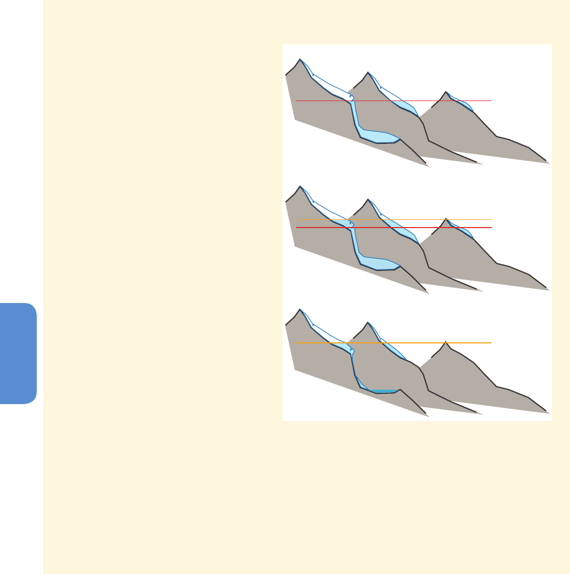
346

Chapter 4 Observations: Cryosphere

FAQ 4.2 (continued)

adjusting its extent to new climatic conditions

and reacts mainly by thinning without substan-

tial terminus retreat. In contrast, smaller moun-

tain glaciers, with fairly constant slopes, adjust

more quickly to the new climate by changing

the size of their ablation area more rapidly

(FAQ 4.2, Figure 1c, middle).

The long-term response of most glacier types

can be determined very well with the approach

illustrated in FAQ 4.2, Figure 1. However, mod-

elling short-term glacier response, or the long-

term response of more complex glacier types

(e.g., those that are heavily debris-covered, fed

by avalanche snow, have a disconnected accu-

mulation area, are of surging type, or calve into

water), is difﬁcult. These cases require detailed

knowledge of other glacier characteristics, such

as mass balance, ice thickness distribution, and

internal hydraulics. For the majority of glaciers

worldwide, such data are unavailable, and

their response to climate change can thus only

be approximated with the simpliﬁed scheme

shown in FAQ 4.2, Figure 1.

The Karakoram–Himalaya mountain range, for

instance, has a large variety of glacier types

and climatic conditions, and glacier character-

istics are still only poorly known. This makes

determining their future evolution particularly

uncertain. However, gaps in knowledge are

expected to decrease substantially in coming

years, thanks to increased use of satellite data

(e.g., to compile glacier inventories or derive

ﬂow velocities) and extension of the ground-

based measurement network.

In summary, the fate of glaciers will be variable,

depending on both their speciﬁc characteristics

and future climate conditions. More glaciers

will disappear; others will lose most of their low-lying portions and others might not change substantially. Where

the ELA is already above the highest elevation on a particular glacier, that glacier is destined to disappear entirely

unless climate cools. Similarly, all glaciers will disappear in those regions where the ELA rises above their highest

elevation in the future.

FAQ 4.2, Figure 1 | Schematic of three types of glaciers located at different elevations,

and their response to an upward shift of the equilibrium line altitude (ELA). (a) For a given

climate, the ELA has a speciﬁc altitude (ELA1), and all glaciers have a speciﬁc size. (b) Due

to a temperature increase, the ELA shifts upwards to a new altitude (ELA2), initially resulting

in reduced accumulation and larger ablation areas for all glaciers. (c) After glacier size has

adjusted to the new ELA, the valley glacier (left) has lost its tongue and the small glacier

(right) has disappeared entirely.

ELA

Valley Glacier

Mountain Glacier

Small Glacier

a) Before climate change

b) After climate change but before glacier readjustment

c) After readjustment to climate change

ELA

a discussion of the improvements in techniques of measurement and

understanding of the change made since AR4 (e.g., Lemke et al., 2007;

Cazenave et al., 2009; Chen et al., 2011).

4.4.2.1 Techniques

The three broad techniques for measuring ice-sheet mass balance are

the mass budget method, repeated altimetry and measurement of

temporal variations in the Earth’s gravity ﬁeld. Each method has been

applied to both ice sheets by multiple groups, and over time scales

ranging from multiple years to decades (Figures 4.13 and 4.14). The

peripheral glaciers, surrounding but not strictly a part of the ice sheets,

are not treated in the same manner by each technique. Peripheral gla-

ciers are generally excluded from estimates using the mass budget

method, they are sometimes, but not always, included in altimetric

estimates, and they are almost always included in gravity estimates.

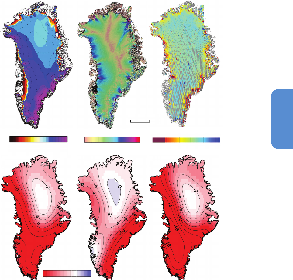
347

Observations: Cryosphere Chapter 4

4.4.2.1.1 Mass budget method

The mass budget method (see Glossary) relies on estimating the dif-

ference between net surface balance over the ice sheet (input) and

perimeter ice discharge ﬂux (output). This method requires compari-

son of two very large numbers, and even small percentage errors in

either may result in large errors in total mass balance. For ice discharge,

perimeter ﬂuxes are calculated from measurements of ice velocity and

ice thickness at the grounding line. Knowledge of perimeter ﬂuxes

has improved signiﬁcantly since AR4 for both ice sheets (Rignot et al.,

2011b) as a result of more complete ice-thickness data (Bamber et

(cm yr

-1

)

-10 -8 -6 -4 -2 0 2 4

2003-2012 2006-20122003-2006

-3 -1 -0.3 0 0.3 1 3

(kg m

-2

-1

) (m yr

-1

)

1 10 100 1000

-1.5 -0.5 -0.2 0 0.2 0.5

(m yr

-1

)

0 500 (km)

(

10 -8 -6 -4 -2

003-2012

006

2012

)

003

2006

Figure 4.13 | Key variable related to the determination of the Greenland ice sheet mass changes. (a) Mean surface mass balance for 1989–2004 from regional atmospheric climate

modelling (Ettema et al., 2009). (b) Ice sheet velocity for 2007–2009 determined from satellite data, showing fastest ﬂow in red, fast ﬂow in blue and slower ﬂow in green and

yellow (Rignot and Mouginot, 2012). (c) Changes in ice sheet surface elevation for 2003–2008 determined from ICESat altimetry, with elevation decrease in red to increase in blue

(Pritchard et al., 2009). (d, e) Temporal evolution of ice loss determined from GRACE time-variable gravity, shown in centimetres of water per year for the periods (a) 2003–2012,

the mass budget method.

al., 2013; Fretwell et al., 2013) and velocity data from satellite radar

interferometry and other techniques (Joughin et al., 2010b; Rignot et

al., 2011a). However, incomplete ice thickness mapping still causes

uncertainties in ice discharge of 2 to 15% in Antarctica (Rignot et al.,

2008b) and 10% in Greenland (Howat et al., 2011; Rignot et al., 2011c).

Regional atmospheric climate models (see Glossary) veriﬁed using

independent in situ data are increasingly preferred to produce esti-

mates of surface mass balance over models that are recalibrated or

corrected with in situ data (Box et al., 2009), downscaling of global

re-analysis data (see Glossary) (Hanna et al., 2011), or interpolation of

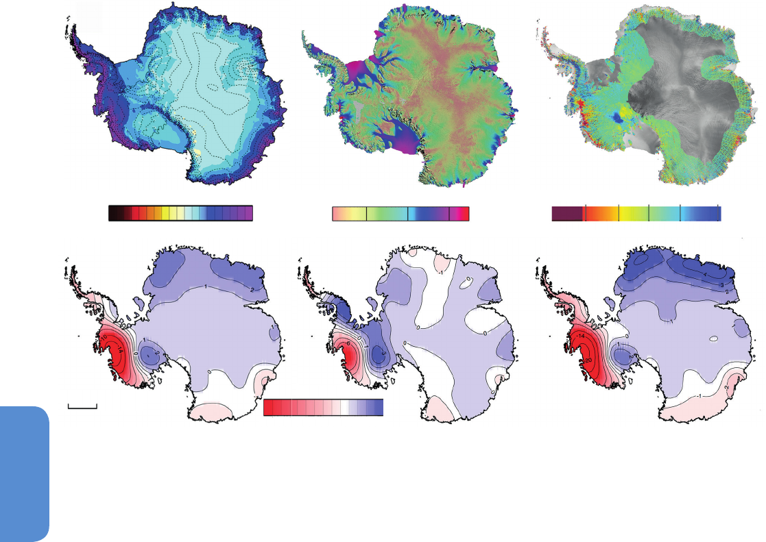
348

Chapter 4 Observations: Cryosphere

Figure 4.14 | Key ﬁelds relating to the determination of Antarctica ice sheet mass changes. (a) Mean surface mass balance for 1989–2004 from regional atmospheric climate

modelling (van den Broeke et al., 2006). (b) Ice sheet velocity for 2007–2009 determined from satellite data, showing fastest ﬂow in red, fast ﬂow in blue, and slower ﬂow in green

and yellow (Rignot et al., 2011a). (c) Changes in ice sheet surface elevation for 2003–2008 determined from ICESat altimetry, with elevation decrease in red to increase in blue

(Pritchard et al., 2009). (d, e) Temporal evolution of ice loss determined from GRACE time-variable gravity, shown in centimetres of water per year for the periods (a) 2003–2012,

the mass budget method.

in situ measurements (Arthern et al., 2006; Bales et al., 2009). In Ant-

arctica, surface mass balance (excluding ice shelves) for 1979–2010 is

estimated at 1983 ± 122 Gt yr

–1

(van de Berg et al., 2006; Lenaerts et

al., 2012) with interannual variability of 114 Gt yr

–1

driven by snow-

fall variability (Figure 4.14). Comparison with 750 in situ observations

indicates an overall uncertainty of 6% for total ice sheet mass balance,

ranging from 5 to 20% for individual drainage basins (van de Berg et

al., 2006; Rignot et al., 2008b; Lenaerts et al., 2012; Shepherd et al.,

2012). In Greenland, total snowfall (697 Gt yr

–1

) and rainfall (46 Gt

–1

) minus runoff (248 Gt yr

–1

) and evaporation/sublimation (26 Gt

–1

) yield a surface mass balance of 469 ± 82 Gt yr

–1

for 1958–2007

(Ettema et al., 2009). The 17% uncertainty is based on a comparison of

model outputs with 350 in situ accumulation observations and, in the

absence of runoff data, an imposed 20% uncertainty in runoff (Howat

et al., 2011). Interannual variability in surface mass balance is large

(107 Gt yr

–1

) due to the out-of-phase relationship between the vari-

ability in precipitation (78 Gt yr

–1

) and runoff (67 Gt yr

–1

4.4.2.1.2 Repeated altimetry

Repeated altimetric survey allows measurement of rates of sur-

face-elevation change, and after various corrections (for changes in

(cm yr

-1

)

-10 -8 -6 -4 -2 0 2 4

(((((((( yyyy ))))

10101010101010 -8-8-8 -6-6-6 -4-4-4 -2-2-2 000 222 44444444-6-6-6

2003-2012 2006-20122003-2006

(kg m

-2

-1

)

1 10 100 1000

-3 -1 -0.3 0 0.3 1 3

(m yr

-1

)

-1.5 -0.5 -0.2 0 0.2 0.5

(m yr

-1

)

0 500 (km)

fed

cba

snow density and bed elevation; or if the ice is ﬂoating, for tides and

sea level) reveals changes in ice sheet mass. Satellite radar altimetry

(SRALT) has been widely used (Thomas et al., 2008b; Wingham et

al., 2009), as has laser altimetry from airplanes (Krabill et al., 2002;

Thomas et al., 2009) and satellites (Pritchard et al., 2009; Abdalati et

al., 2010; Sorensen et al., 2011; Zwally et al., 2011). Both radar and

laser methods have signiﬁcant challenges. The ﬁeld-of-view of early

SRALT sensors was ~20 km in diameter, and as a consequence, inter-

pretation of the data they acquired over ice sheets with undulating

surfaces or signiﬁcant slopes was complex. Also, for radar altimeters,

estimates are affected by penetration of the radar signal below the

surface, which depends on characteristics such as snow density and

wetness, and by wide orbit separation (Thomas et al., 2008b). Errors

in surface-elevation change are typically determined from the internal

consistency of the measurements, often after iterative removal of sur-

face elevation-change values that exceed some multiple of the local

value of their standard deviation; this results in very small error esti-

mates (Zwally et al., 2005).

Laser altimeters have been used from aircraft for many years, but satel-

lite laser altimetry, available for the ﬁrst time from NASA’s ICESat satel-

lite launched in 2003, has provided many new results since AR4. Laser

349

Observations: Cryosphere Chapter 4

altimetry is easier to validate and interpret than radar data; the ﬁeld of

view is small (1 m diameter for airborne lasers, 60 m for ICESat), and

there is negligible penetration below the surface. However, clouds limit

data acquisition, and accuracy is affected by atmospheric conditions,

laser-pointing errors, and data scarcity.

Knowledge of the density of the snow and ﬁrn in the upper layers of

an ice sheet is required to convert altimetric measurements to mass

change. However, snow densiﬁcation rates are sensitive to snow tem-

perature and wetness. Warm conditions favour more rapid densiﬁca-

tion (Arthern et al., 2010; Li and Zwally, 2011). Consequently, recent

Greenland warming has probably caused surface lowering simply from

this effect. Corrections are inferred from models that are difﬁcult to

validate and are typically less than 2 cm yr

–1

. ICESat derived surface

elevation changes supplemented with differenced ASTER (Advanced

Spaceborne Thermal Emission and Reﬂection Radiometer) satellite

digital elevation models were used for outlet glaciers in southeast

Greenland (Howat et al., 2008) and for the northern Antarctic Penin-

sula (Shuman et al., 2011). Laser surveys from airborne platforms over

Greenland yield elevation estimates accurate to 10 cm along reference

targets (Krabill et al., 1999; Thomas et al., 2009) and 15 cm for ICESat

using ground-based high-resolution GPS measurements (Siegfried et

al., 2011). For a 5-year separation between surveys, this is an uncer-

tainty of 2.0 cm yr

–1

for airborne platforms and 3 cm yr

–1

for ICESat.

Early in 2013, NASA released an elevation correction for ICESat

(National Snow and Ice Data Center, 2013) that is relevant to several

studies cited in this chapter, but was provided too late to be includ-

ed in those studies. This correction improves shot-to-shot variability

in ICESat elevations, although spatial averaging and application of

inter-campaign bias corrections derived from calibration data and used

in many studies already mitigates the impact of the higher variability.

The correction also changes elevation trend estimates over the 2003–

2009 ICESat mission period by up to –1.4 cm yr

–1

To date, a thorough treatment of the impact of this ﬁnding has not

been published in the peer-reviewed literature, but the overall magni-

tude of the effect is reported to be at the level of 1.4 cm yr

–1

. For many

studies of glaciers, ice sheets and sea ice this is substantially lower (in

some cases, an order of magnitude lower) than the signal of change,

but elsewhere (e.g, for elevation changes in East Antarctica) it may

have an impact. However, multiple lines of evidence, of which ICESat is

only one, are used to arrive at the conclusions presented in this chapter.

To the degree to which it can be assessed, there is high conﬁdence

that the substantive conclusions this chapter will not be affected by

revisions of the ICESat data products.

4.4.2.1.3 Temporal variations in Earth gravity ﬁeld

Since 2002, the GRACE (Gravity Recovery and Climate Experiment)

satellite mission has surveyed the Earth’s time-variable gravity ﬁeld.

Time-variable gravity provides a direct estimate of the ice-mass

change at a spatial resolution of about 300 km (Wahr, 2007). GRACE

data yielded early estimates of trends in ice-mass changes over the

Greenland and Antarctic ice sheets and conﬁrmed regions of ice loss in

coastal Greenland and West Antarctica (Luthcke et al., 2006; Velicogna

and Wahr, 2006a, 2006b). With extended time series, now more than

10 years, estimates of ice sheet mass change from GRACE have lower

uncertainties than in AR4 (e.g., Harig and Simons, 2012; King et al.,

2012). The ice-loss signal from the last decade is also more distinct

because the numbers have grown signiﬁcantly higher (e.g., Wouters

et al., 2008; Cazenave et al., 2009; Chen et al., 2009; Velicogna, 2009).

The estimates of ice loss based on data from GRACE vary between pub-

lished studies due to the time-variable nature of the signal, along with

other factors that include (1) data-centre speciﬁc processing, (2) specif-

ic methods used to calculate the mass change, and (3) contamination

by other signals within the ice sheet (e.g., glacial isostatic adjustment

or GIA, see Glossary) or outside the ice sheet (continental hydrology,

ocean circulation). Many of these differences have been reduced in

studies published since AR4, resulting in greater agreement between

GRACE estimates (Shepherd et al., 2012).

In Antarctica, the GIA signal is similar in magnitude to the ice-loss

signal, with an uncertainty of ±80 Gt yr

–1

(Velicogna and Wahr, 2006b;

Riva et al., 2009; Velicogna, 2009). Correction for the GIA signal is

addressed using numerical models (e.g., Ivins and James, 2005; Paul-

son et al., 2007; Peltier, 2009). A comparison of recent GIA models

(Tarasov and Peltier, 2002; Fleming and Lambeck, 2004; Peltier, 2004;

Ivins and James, 2005; Simpson et al., 2009; Whitehouse et al., 2012)

with improved constraints on ice-loading history, indicate better agree-

ment with direct observations of vertical land movements (Thomas et

al., 2011a), despite a potential discrepancy between far-ﬁeld sea level

records and common NH deglaciation models. In Greenland, the GIA

correction is less than 10% of the GRACE signal with an error of ±19

Gt yr

–1

. However, because the GIA rate is constant over the satellite’s

lifetime, GIA uncertainty does not affect the estimate of any change in

the rate of ice mass loss (acceleration/deceleration). In Antarctica, the

adoption of new GIA models has resulted in a lowering of estimated

ice-sheet mass loss (King et al., 2012; Shepherd et al., 2012).

In addition to GRACE, the elastic response of the crustal deformation

shown in GPS measurements of uplift rates conﬁrms increasing rates

of ice loss in Greenland (Khan et al., 2010b; Khan et al., 2010a) and

Antarctica (Thomas et al., 2011a). Analysis of a 34-year time series

of the Earth’s oblateness (J2) by satellite laser ranging also suggests

that ice loss from Greenland and Antarctica has progressively dom-

inated the change in oblateness trend since the 1990s (Nerem and

Wahr, 2011).

4.4.2.2 Greenland

There is very high conﬁdence that the Greenland ice sheet has lost ice

and contributed to sea level rise over the last two decades (Ewert et al.,

2012; Sasgen et al., 2012; Shepherd et al., 2012). Recent GRACE results

are in better agreement than in AR4 as discussed in Section 4.4.2.1

(Baur et al., 2009; Velicogna, 2009; Pritchard et al., 2010; Wu et al.,

2010; Chen et al., 2011; Schrama and Wouters, 2011). Altimetry mis-

sions report losses comparable to those from the mass budget method

and from the time-variable gravity method (Thomas et al., 2006; Zwally

et al., 2011) (Figure 4.13f).

Figure 4.15 shows the cumulative ice mass loss from the Greenland

ice sheet over the period 1992–2012 derived from 18 recent studies

made by 14 different research groups (Baur et al., 2009; Cazenave et

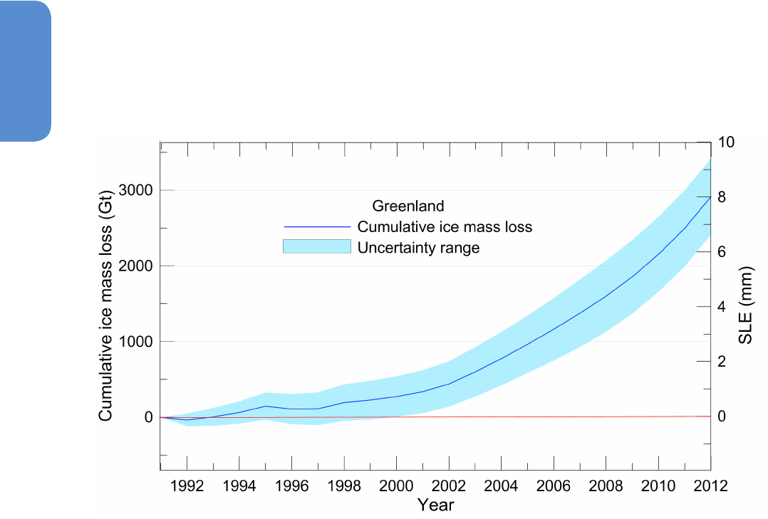
350

Chapter 4 Observations: Cryosphere

al., 2009; Slobbe et al., 2009; Velicogna, 2009; Pritchard et al., 2010;

Wu et al., 2010; Chen et al., 2011; Rignot et al., 2011c; Schrama and

Wouters, 2011; Sorensen et al., 2011; Zwally et al., 2011; Ewert et al.,

2012; Harig and Simons, 2012; Sasgen et al., 2012). These studies do

not include earlier estimates from the same researchers when those

have been updated by more recent analyses using extended data. They

include estimates made from satellite gravimetry, satellite altimetry

and the mass budget method. Details of the studies used for Greenland

are listed in Appendix Table 4.A.1 (additional studies not selected are

listed in Table 4.A.2).

The mass balance for each year is estimated as a simple average of all

the selected estimates available for that particular year. Figure 4.15

shows an accumulation of these estimates since an arbitrary zero on 1

January 1992. The number of estimates available varies with time, with

as few as two estimates per year in the 1990s and up to 18 per year

from 2004. The cumulative uncertainty in Figure 4.15 is based on the

uncertainty cited in the original studies which, when the conﬁdence

level is not speciﬁcally given, is assumed to be at the 1 standard devi-

ation (1σ) level. However, the annual estimates from different studies

often do not overlap within the original uncertainties, and hence the

error limits used in this assessment are derived from the absolute max-

imum and minimum mass balance estimate for each year. These have

been converted to the 90% conﬁdence interval (5 to 95%, or 1.65σ).

The cumulative error is weighted by 1/√n , where n is the number of

years accumulated.

Despite year-to-year differences between the various original analyses,

this multi-study assessment yields very high conﬁdence that Green-

land has lost mass over the last two decades and high conﬁdence that

the rate of loss has increased. The increase is also shown in several

Figure 4.15 | Cumulative ice mass loss (and sea level equivalent, SLE) from Greenland derived as annual averages from 18 recent studies (see main text and Appendix 4.A for

details).

individual studies (Velicogna, 2009; Chen et al., 2011; Rignot et al.,

2011c; Zwally et al., 2011) (Figure 4.13a–c). The average ice mass

change to Greenland from the present assessment has been –121

[–149 to –94] Gt yr

–1

(a sea level equivalent of 0.33 [0.41 to 0.26]

mm yr

–1

) over the period 1993 to 2010, and –229 [–290 to –169] Gt

–1

(0.63 [0.80 to 0.47] mm yr

–1

sea level equivalent) over the period

2005–2010.

Greenland changes that include and exclude peripheral glaciers cannot

be cleanly separated from the mixture of studies and techniques in this

assessment, but for the post 2003 period there is a prevalence of grav-

ity studies, which do include the peripheral glaciers. Hence, although

the estimated mass change in Greenland peripheral glaciers of –38 ± 7

Gt yr

–1

over the period 2003–2009 (Gardner et al., 2013) is discussed in

Section 4.3.3 (Table 4.5), these changes are included within the values

for ice-sheet change quoted in this section, and not as part of the total

mass change for glaciers.

A reconciliation of apparent disparities between the different satel-

lite methods was made by the Ice-sheet Mass Balance Intercompari-

son Experiment (IMBIE) (Shepherd et al., 2012). This intercomparison

combined an ensemble of satellite altimetry, interferometry, airborne

radio-echo sounding and airborne gravimetry data and regional

atmospheric climate model output products, for common geographical

regions and for common time intervals. Good agreement was obtained

between the estimates from the different methods and, whereas the

uncertainties of any method are sometimes large, the combination of

methods considerably improves the overall certainty. (Note that Shep-

herd et al. (2012) also cannot cleanly separate estimates including or

excluding peripheral glaciers). For Greenland, Shepherd et al. (2012)

estimate a change in mass over the period 1992–2011, averaged

351

Observations: Cryosphere Chapter 4

across the ensemble for each method, of –142 ± 49 Gt yr

–1

(0.39 ±

0.14 mm yr

–1

of sea level rise). For the same period, this present assess-

ment, which averages across individual studies, yields a slightly slower

loss, with a rate of mass change of –125 ± 25 Gt yr

–1

at the 90% con-

ﬁdence level (0.34 ± 0.07 mm yr

–1

SLE). Averaging across technique

ensembles in the present assessment yields a loss at a rate of –129 Gt

–1

(0.36 mm). Shepherd et al. (2012) conﬁrm an increasing mass loss

from Greenland, although they also identify mass balance variations

over intermediate (2- to 4-year) periods.

The mass budget method shows that ice loss from the Greenland ice

sheet is partitioned in approximately similar amounts between sur-

face mass balance (i.e., runoff) and discharge from ice ﬂow across the

grounding line (van den Broeke et al., 2009) (medium conﬁdence).

However, there are signiﬁcant differences in the relative importance

of ice discharge and surface mass balance in various regions of Green-

land (Howat et al., 2007; Pritchard et al., 2009; van den Broeke et al.,

2009; Sasgen et al., 2012). Dynamic losses dominate in southeast and

central west regions, and also inﬂuence losses in northwest Greenland,

whereas in the central north, southwest and northeast sectors, chang-

es in surface mass balance appear to dominate.

There is high conﬁdence that over the last two decades, surface mass

balance has become progressively more negative as a result of an

increase in surface melt and runoff, and that ice discharge across the

grounding line has also been enhanced due to the increased speed

of some outlet glaciers. Altimetric measurements of surface height

suggest slight inland thickening in 1994–2006 (Thomas et al., 2006,

2009), but this is not conﬁrmed by regional atmospheric climate model

outputs for the period 1957–2009 (Ettema et al., 2009), nor recent ice

core (see Glossary) data (Buchardt et al., 2012), hence there is low

conﬁdence in an increase in precipitation in Greenland in recent dec-

ades. Probable changes in accumulation are, however, exceeded by the

increased runoff especially since 2006 (van den Broeke et al., 2009).

The four highest runoff years over the last 140 years occurred since

1995 (Hanna et al., 2011).

The total surface melt area has continued to increase since AR4 and

has accelerated in the past few years (Fettweis et al., 2011; Tedesco

et al., 2011), with an extreme melt event covering more than 90% of

the ice sheet for a few days in July 2012 (Nghiem et al., 2012; Tedesco

et al., 2013). Annual surface mass balance in 2011–2012 was 2 stand-

ard deviations (2σ) below the 2003–2012 mean. Such extreme melt

events are rare and have been observed in ice core records only twice,

once in 1889, and once more, seven centuries earlier in the Medieval

Warm Period (Meese et al., 1994; Alley and Anandakrishnan, 1995).

Over the past decade, the surface albedo of the Greenland ice sheet

has decreased by up to 18% in coastal regions, with a statistically

signiﬁcant increase over 87% of the ice sheet due to melting and snow

metamorphism, allowing more solar energy to be absorbed for surface

melting (Box et al., 2012).

GRACE results show ice loss was largest in southeast Greenland during

2005 and increased in the northwest after 2007 (Khan et al., 2010a;

Chen et al., 2011; Schrama and Wouters, 2011; Harig and Simons,

2012). Subsequent to 2005, ice loss decreased in the southeast. These

GRACE results agree with measurements of ice discharge from the

major outlet glaciers that conﬁrm the dominance of dynamic losses in

these regions (van den Broeke et al., 2009). In particular, major outlet

glacier speed-up reported in AR4 occurred in west Greenland between

1996 and 2000 (Rignot and Kanagaratnam, 2006) and in southeast

Greenland from 2001 to 2006 (Rignot and Kanagaratnam, 2006;

Joughin et al., 2010b). In the southeast, many outlet glaciers slowed

after 2005 (Howat et al., 2007; Howat et al., 2011), with many ﬂow

speeds decreasing back towards those of the early 2000s (Murray et

al., 2010; Moon et al., 2012), although most are still ﬂowing faster and

discharging more ice into the ocean than they did in 1996 (Rignot and

Kanagaratnam, 2006; Howat et al., 2011).

In the northwest, the increase in the rate of ice loss from 1996–2006 to

2006–2010 was probably caused partially by a higher accumulation in

the late 1990s compared to earlier and later years (Sasgen et al., 2012),

but ice dynamic changes also played a role as outlet glaciers in the

northwest showed an increase in speed from 2000 to 2010, with the

greatest increase from 2007 to 2010 (Moon et al., 2012). Longer-term

observations of surface topography in the northwest sector conﬁrm

the dynamic component of this mass loss and suggest two periods of

loss in 1985–1993 and 2005–2010 separated by limited mass changes

(Kjaer et al., 2012). In the southeast, an 80-year long record reveals

that many land-terminating glaciers retreated more rapidly in the

1930s compared to the 2000s, but marine-terminating glaciers retreat-

ed more rapidly during the recent warming (Bjørk et al., 2012).

4.4.2.3 Antarctica

Antarctic results from the gravity method are also now more numerous

and consistent than in AR4 (Figure 4.14a-c). Methods combining GPS

and GRACE at the regional level indicate with high conﬁdence that

the Antarctic Peninsula is losing ice (Ivins et al., 2011; Thomas et al.,

2011a). In other areas, large uncertainties remain in the global GRACE-

GPS solutions (Wu et al., 2010).

The SMB reconstructions used in the mass budget method have

improved considerably since AR4 (e.g., Rignot et al. 2008b; van den

Broeke et al., 2006; Lenaerts et al., 2012; Shepherd et al., 2012). Recon-

structed snowfall from regional atmospheric climate models indicates

higher accumulation along the coastal sectors than in previous esti-

mates, but little difference in total snowfall. There is medium conﬁdence

that there has been no long-term trend in the total accumulation over

the continent over the past few decades (Monaghan et al., 2006; van

den Broeke et al., 2006; Bromwich et al., 2011; Frezzotti et al., 2012;

Lenaerts et al., 2012). Although anomalies in accumulation have been

noted in recent decades in Eastern Wilkes Land (Boening et al., 2012;

Shepherd et al., 2012) and Law Dome (Van Ommen and Morgan, 2010)

in East Antarctica, their overall impact on total mass balance is not sig-

niﬁcant. Satellite laser altimetry indicates that ice volume changes are

concentrated on outlet glaciers and ice streams (see Glossary), as illus-

trated by the strong correspondence between areas of thinning (Figure

4.14f) and areas of fast ﬂow (Figure 4.14e) (Pritchard et al., 2009).

Figure 4.16 shows the cumulative ice mass loss from the Antarctic ice

sheet over the period 1992–2012 derived from recent studies made

by 10 different research groups (Cazenave et al., 2009; Chen et al.,

2009; E et al., 2009; Horwath and Dietrich, 2009; Velicogna, 2009; Wu

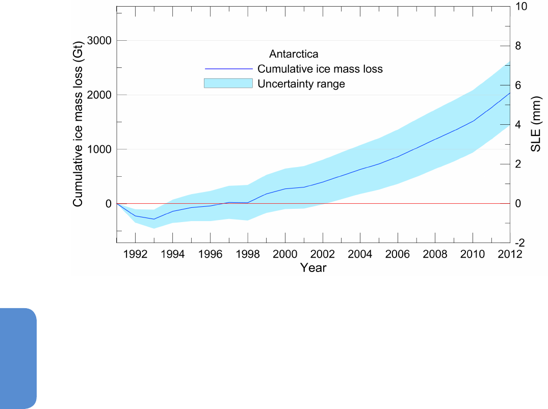
352

Chapter 4 Observations: Cryosphere

et al., 2010; Rignot et al., 2011c; Shi et al., 2011; King et al., 2012; Tang

et al., 2012). These studies do not include earlier estimates from the

same researchers when those have been updated by more recent anal-

yses using extended data. They include estimates made from satellite

gravimetry, satellite altimetry and the mass balance method. Details

of the studies used for Antarctica are listed in Table 4.A.3 (additional

studies not selected are listed in Table 4.A.4). The number of estimates

available varies with time, with only one estimate per year in the 1990s

and up to 10 per year from 2003. The cumulative curves and associated

errors are derived in the same way as those for Figure 4.15 (see Section

4.4.2.2).

Overall, there is high conﬁdence that the Antarctic ice sheet is current-

ly losing mass. The average ice mass change to Antarctica from the

present assessment has been –97 [–135 to –58] Gt yr

–1

(a sea level

equivalent of 0.27 mm yr

–1

[0.37 to 0.16] mm yr

–1

) over the period

1993–2010, and –147 [–221 to –74] Gt yr

–1

(0.41 [0.61 to 0.20] mm

–1

) over the period 2005–2010. These assessments include the Ant-

arctic peripheral glaciers.

The recent IMBIE intercomparison (Shepherd et al., 2012) for Antarc-

tica, where the GIA signal is less well known than in Greenland, used

two new GIA models (an updated version of Ivins and James (2005),

for details see Shepherd et al. (2012); and Whitehouse et al. (2012)).

These new models had the effect of reducing the estimates of East Ant-

arctic ice mass loss from GRACE data, compared with some previous

estimates. For Antarctica, Shepherd et al. (2012) estimate an average

change in mass for 1992–2011 of –71 ± 53 Gt yr

–1

(0.20 ± 0.15 mm

–1

of sea level equivalent). For the same period this present assess-

ment estimates a loss of 88 ± 35 Gt yr

–1

at the 90% conﬁdence level

(0.24 ± 0.10 mm yr

–1

SLE). Averaging across technique ensembles in

Figure 4.16 | Cumulative ice mass loss (and sea level equivalent, SLE) from Antarctica derived as annual averages from 10 recent studies (see main text and Appendix 4.A for

details).

the present assessment, rather than individual estimates, yields no sig-

niﬁcant difference.

There is low conﬁdence that the rate of Antarctic ice loss has increased

over the last two decades (Chen et al., 2009; Velicogna, 2009; Rignot et

al., 2011c; Shepherd et al., 2012); however, GRACE data gives medium

conﬁdence of increasing loss over the last decade (Chen et al., 2009;

Velicogna, 2009) (Figure 4.16). For GRACE, this conclusion is independ-

ent of the GIA signal, which is constant over the measurement period.

The mass budget method suggests that the increase in loss from the

mass budget method is caused by an increase in glacier ﬂow-speed

in the eastern part of the Paciﬁc sector of West Antarctica (Rignot,

2008; Joughin et al., 2010a) and the Antarctic Peninsula (Scambos et

al., 2004; Pritchard and Vaughan, 2007; Rott et al., 2011). Comparison

of GRACE and the mass budget method for 1992–2010 indicates an

increase in the rate of ice loss of, on average, 14 ± 2 Gt yr

–1

per year

compared with 21 ± 2 Gt yr

–1

per year on average for Greenland during

the same time period (Rignot et al., 2011c). The recent IMBIE analysis

(Shepherd et al., 2012) shows that the West Antarctic ice sheet and the

Antarctic Peninsula are losing mass at an increasing rate, but that East

Antarctica gained an average of 21 ± 43 Gt yr

–1

between 1992 and

2011. Zwally and Giovinetto (2011) also estimate a mass gain for East

Antarctica (+16 Gt yr

–1

between 1992 and 2001). Their reassessment

of total Antarctic change made a correction for the ice discharge esti-

mates from regions of the ice sheet not observed in the mass budget

method (see Section 4.4.2.1.1). The analysis of Shepherd et al. (2012)

indicated that the missing regions contribute little to the total mass

change.

In the near-absence of surface runoff and, as discussed in this section,

with no evidence of multi-decadal change in total snowfall, there is

353

Observations: Cryosphere Chapter 4

high conﬁdence that Antarctic multi-decadal changes in grounded ice

mass must be due to increased ice discharge, although the observation-

al record of ice dynamics extends only from the 1970s and is spatially

incomplete for much of this period. Over shorter time scales, howev-

er, the interannual to decadal variability in snowfall has an important

impact on ice sheet mass balance (Rignot et al., 2011c).

The three techniques are in excellent agreement as to the spatial pat-

tern of ice loss (thinning) and gain (thickening) over Antarctica (Figure

4.14). There is very high conﬁdence that the largest ice losses are locat-

ed along the northern tip of the Antarctic Peninsula where the collapse

of several ice shelves in the last two decades triggered the acceleration

of outlet glaciers, and in the Amundsen Sea, in West Antarctica (Figure

4.14).. On the Antarctic Peninsula, there is evidence that precipita-

tion has increased (Thomas et al., 2008a) but the resulting ice-gain

is insufﬁcient to counteract the losses (Wendt et al., 2010; Ivins et al.,

2011). There is medium conﬁdence that changes in the Amundsen Sea

region are due to the thinning of ice shelves (Pritchard et al., 2012),

and medium conﬁdence that this is due to high ocean heat ﬂux (Jacobs

et al., 2011), which caused grounding line retreat (1 km yr

–1

) (Joughin

et al., 2010a) and glacier thinning (Wingham et al., 2009). Indications

of dynamic change are also evident in East Antarctica, primarily around

Totten Glacier, from GRACE (Chen et al., 2009), altimetry (Wingham

et al., 2006; Shepherd and Wingham, 2007; Pritchard et al., 2009; Fla-

ment and Remy, 2012), and satellite radar interferometry (Rignot et

al., 2008b). The contribution to the total ice loss from these areas is,

however, small and not well understood.

4.4.2.4 Ice Shelves and Floating Ice Tongues

As much as 74% of the ice discharged from the grounded ice sheet in

Antarctica passes through ice shelves and ﬂoating ice tongues (Bind-

schadler et al., 2011). Ice shelves help to buttress and restrain ﬂow of

the grounded ice (Rignot et al., 2004; Scambos et al., 2004; Hulbe et al.,

2008), and so changes in thickness (Shepherd et al., 2003, 2010; Fricker

and Padman, 2012), and extent (Doake and Vaughan, 1991; Scambos

et al., 2004) of ice shelves inﬂuence current ice sheet change. Indeed,

nearly all of the outlet glaciers and ice streams that are experiencing

high rates of ice loss ﬂow into thinning or disintegrated ice shelves

(Pritchard et al., 2012). Many of the larger ice shelves however, exhibit

stable conditions (King et al., 2009; Shepherd et al., 2010; Pritchard et

al., 2012).

Around the Antarctic Peninsula, the reduction in ice-shelf extent has

been ongoing for several decades (Cook and Vaughan, 2010; Fricker

and Padman, 2012), and has continued since AR4 with substantial col-

lapse of a section of Wilkins Ice Shelf (Humbert et al., 2010), which had

been retreating since the late1990s (Scambos et al., 2000). Overall, 7 of

12 ice shelves around the Peninsula have retreated in recent decades

with a total loss of 28,000 km

, and a continuing rate of loss of around

6000 km

per decade (Cook and Vaughan, 2010). There is high conﬁ-

dence that this retreat of ice shelves along the Antarctic Peninsula has

been related to changing atmospheric temperatures (e.g., Scambos et

al., 2000; Morris and Vaughan, 2003; Marshall et al., 2006; Holland et

al., 2011). There is low conﬁdence that changes in the ocean have also

contributed (e.g., Shepherd et al., 2003; Holland et al., 2011; Nicholls

et al., 2012; Padman et al., 2012).

4.4.3 Total Ice Loss from Both Ice Sheets

The total ice loss from both ice sheets for the 20 years 1992–2011

(inclusive) has been 4260 [3060 to 5460] Gt, equivalent to 11.7 [8.4

to 15.1] mm of sea level. However, the rate of change has increased

with time and most of this ice has been lost in the second decade of

the 20-year period. From the data presented in Figure 4.17, the average

loss in Greenland has very likely increased from 34 [–6 to 74] Gt yr

–1

over the decade 1992–2001 (sea level equivalent, 0.09 [–0.02 to 0.20]

mm yr

–1

), to 215 [157 to 274] Gt yr

–1

over the decade 2002–2011 (0.59

[0.43 to 0.76] mm yr

–1

). In Antarctica, the loss has likely increased 30

[–37 to 97] Gt yr

–1

(sea level equivalent, 0.08 [–0.10 to 0.27] mm yr

–1

)

for 1992–2001, to 147 [72 to 221] Gt yr

–1

for 2002–2011 (0.40 [0.20

to 0.61] mm yr

–1

). Over the last ﬁve years (2007–2011), the loss from

both ice sheets combined has been equivalent to 1.2 ± 0.4 mm yr

–1

sea level (Figure 4.17 and Table 4.6).

4.4.4 Causes of Changes in Ice Sheets

4.4.4.1 Climatic Forcing

Changes in ice sheet mass balance are the result of an integrated

response to climate, and it is imperative that we understand the con-

text of current change within the framework of past changes and nat-

ural variability.

4.4.4.1.1 Snowfall and surface temperature

Ice sheets experience large interannual variability in snowfall, and local

trends may deviate signiﬁcantly from the long-term trend in integrated

snowfall. However, as in AR4, the available data do not suggest any

signiﬁcant long-term change in accumulation in Antarctica, except for

the Antarctic Peninsula (Monaghan et al., 2006; Ettema et al., 2009;

van den Broeke et al., 2009; Bromwich et al., 2011).

Increasing air temperature will (when above the freezing point)

increase the amount of surface melt, and can also increase the mois-

ture bearing capacity of the air, and hence can increase snowfall. Over

Greenland, temperature has risen signiﬁcantly since the early 1990s,

reaching values similar to those in the 1930s (Box et al., 2009). The

Period

Ice sheet loss

(mm yr

–1

SLE)

Greenland

2005–2010 (6-year) 0.63 ±0.17

1993–2010 (18-year) 0.33 ±0.08

Antarctica

2005–2010 (6-year) 0.41 ±0.20

1993–2010 (18-year) 0.27 ±0.11

Combined

2005–2010 (6-year) 1.04 ±0.37

1993–2010 (18-year) 0.60 ±0.18

Table 4.6 | Average rates of ice sheet loss given as mm of sea level equivalent, derived

as described for Figure 4.15 and Figure 4.16 using estimates listed in Appendix Tables

4.A.1 and 4.A.3.

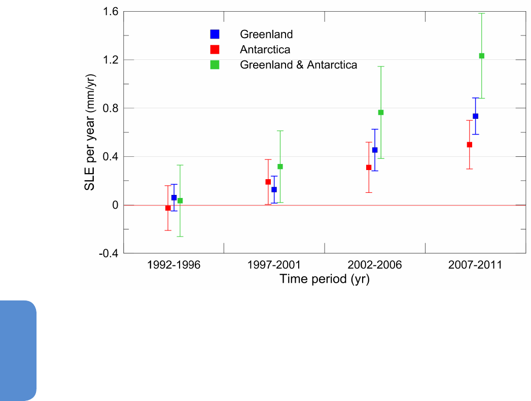
354

Chapter 4 Observations: Cryosphere

Figure 4.17 | Rate of ice sheet loss in sea level equivalent averaged over 5-year periods between 1992 and 2011. These estimates are derived from the data in Figures 4.15 and

4.16.

year 2010 was an exceptionally warm year in west Greenland with

Nuuk having the warmest year since the start of the temperature

record in 1873 (Tedesco et al., 2011). In West Antarctica, the warming

since the 1950s (Steig et al., 2009; Ding et al., 2011; Schneider et al.,

2012; Bromwich et al., 2013), the magnitude and seasonality of which

are still debated, has not manifested itself in enhanced surface melt-

ing (Tedesco and Monaghan, 2009; Kuipers Munneke et al., 2012) nor

in increased snowfall (Monaghan et al., 2006; Bromwich et al., 2011;

Lenaerts et al., 2012). Statistically signiﬁcant summer warming has

been observed on the east coast of the northern Antarctic Peninsula

(Marshall et al., 2006; Chapman and Walsh, 2007), with extension of

summer melt duration (Barrand et al., 2013), while East Antarctica has

showed summer cooling (Turner et al., 2005). In contrast, the signiﬁ-

cant winter warming at Faraday/Vernadsky station on the western Ant-

arctic Peninsula is attributable to a reduction of sea ice extent (Turner

et al., 2005).

4.4.4.1.2 Ocean thermal forcing

Since AR4, observational evidence has contributed to medium conﬁ-

dence that the interaction between ocean waters and the periphery

of large ice sheets plays a major role in present ice sheet changes

(Holland et al., 2008; Pritchard et al., 2012). Ocean waters provide the

heat that can drive high melt rates beneath ice shelves (Jacobs et al.,

1992; Holland and Jenkins, 1999; Rignot and Jacobs, 2002; Pritchard

et al., 2012) and at marine-terminating glacier fronts (Holland et al.,

2008; Rignot et al., 2010; Jacobs et al., 2011).

Ocean circulation delivers warm waters to ice sheets. Variations in

wind patterns associated with the North Atlantic Oscillation (Jacobs

et al., 1992; Hurrell, 1995), and tropical circulations inﬂuencing West

Antarctica (Ding et al., 2011; Steig et al., 2012), are probable drivers of

increasing melt at some ice-sheet margins. In some parts of Antarctica,

changes in the Southern Annular Mode (Thompson and Wallace, 2000,

see Glossary) may also be important. Observations have established

that warm waters of subtropical origin are present within several fjords

in Greenland (Holland et al., 2008; Myers et al., 2009; Straneo et al.,

2010; Christoffersen et al., 2011; Daniault et al., 2011).

Satellite records and in situ observations indicate warming of the

Southern Ocean (see Chapter 3) since the 1950s (Gille, 2002, 2008).

This warming is conﬁrmed by data from robotic ocean buoys (Argo

ﬂoats) (Boening et al., 2008) but the observational record remains

short and, close to Antarctica, there are only limited observations from

ships (Jacobs et al., 2011), short-duration moorings and data from

instrumented seals (Charrassin et al., 2008; Costa et al., 2008).

4.4.4.2 Ice Sheet Processes

4.4.4.2.1 Basal lubrication

Ice ﬂows in part by sliding over the underlying rock and sediment,

which is lubricated by water at the ice base: a process known as basal

lubrication (see Glossary). In many regions close to the Greenland ice

sheet margin, abundant summer meltwater on the surface of the ice

sheet forms large lakes. This surface water can drain to the ice sheet

355

Observations: Cryosphere Chapter 4

bed, thus increasing basal water pressure, reducing basal friction and

increasing ice ﬂow speed (Zwally et al., 2002b).

Such drainage events are common in southwest and northeast Green-

land, but rare in the most rapidly changing southeast and northwest

regions (Selmes et al., 2011). The effect can be seen in diurnal ﬂow var-

iations of some land-terminating regions (Das et al., 2008; Shepherd et

al., 2009), and after lake-drainage events, when 50 to 110% short-term

speed-up of ﬂow has been observed. However, the effect is temporally

and spatially restricted (Das et al., 2008). The summer increase in speed

over the annual mean is only ~10–20%, the increase is less at higher

elevations (Bartholomew et al., 2011), and observations suggest most

lake drainages do not affect ice sheet velocity (Hoffman et al., 2011).

Theory and ﬁeld studies suggest an initial increase in ﬂow rate with

increased surface meltwater supply (Bartholomew et al., 2011; Palmer

et al., 2011), but if the supply of surface water continues to increase

and subglacial drainage becomes more efﬁcient, basal water pressure,

and thus basal motion, is reduced (van de Wal et al., 2008; Schoof,

2010; Sundal et al., 2011; Shannon et al., 2012). Overall, there is high

conﬁdence that basal lubrication is important in modulating ﬂow in

some regions, especially southwest Greenland, but there is also high

conﬁdence that it does not explain recent dramatic regional speed-ups

that have resulted in rapid increases in ice loss from calving glaciers.

4.4.4.2.2 Cryo-hydrologic warming

Percolation and refreezing of surface meltwater that drains through

the ice column may alter the thermal regime of the ice sheet on decad-

al time scales (Phillips et al., 2010). This process is known as cryo-hy-

drologic warming, and it could affect ice rheology and hence ice ﬂow.

4.4.4.2.3 Ice shelf buttressing

Recent changes in marginal regions of the Greenland and Antarctic ice

sheets include some thickening and slowdown of outlet glaciers, but

mostly thinning and acceleration (e.g., Pritchard et al., 2009; Sorensen

et al., 2011), with some glacier speeds increasing two- to eight-fold

(Joughin et al., 2004; Rignot et al., 2004; Scambos et al., 2004; Luck-

man and Murray, 2005; Rignot and Kanagaratnam, 2006; Howat et al.,

2007). Many of the largest and fastest glacier changes appear to be

at least partly a response to thinning, shrinkage or loss of ice shelves

or ﬂoating ice tongues (MacGregor et al., 2012; Pritchard et al., 2012).

This type of glacier response is consistent with classical models of ice

shelf buttressing proposed 40 years ago (Hughes, 1973; Weertman,

1974; Mercer, 1978; Thomas and Bentley, 1978).

4.4.4.2.4 Ice–ocean interaction

Since AR4 it has become far more evident that the rates of subma-

rine melting can be very large (e.g., Motyka et al., 2003). The rate of

melting is proportional to the product of ocean thermal forcing (dif-

ference between ocean temperature and the in situ freezing point of

seawater) and water ﬂow speed at the ice–ocean interface (Holland

and Jenkins, 1999). Melt rates along marine-terminating glacier mar-

gins are one-to-two orders of magnitude greater than for ice shelves

because of the additional buoyancy forces provided by the discharge

of sub-glacial melt water at the glacier base (Motyka et al., 2003; Jen-

kins, 2011; Straneo et al., 2012; Xu et al., 2012). In South Greenland,

there is medium conﬁdence that the acceleration of glaciers from the

mid-1990s to mid-2000s was due to the intrusion of ocean waters of

subtropical origin into glacial fjords (Holland et al., 2008; Howat et al.,

2008; Murray et al., 2010; Straneo et al., 2010; Christoffersen et al.,

2011; Motyka et al., 2011; Straneo et al., 2011; Rignot and Mouginot,

2012). Models suggest that the increase in ice melting by the ocean

contributed to the reduction of backstress experienced by glaciers and

subsequent acceleration (Payne et al., 2004; Schoof, 2007; Nick et al.,

2009; Nick et al., 2013; O’Leary and Christoffersen, 2013): changes in

the ﬂoating mixture of sea ice, iceberg debris and blown snow in front

of the glacier may also play a part (Amundson et al., 2010).

4.4.4.2.5 Iceberg calving

Calving of icebergs from marine-terminating glaciers and ice shelves

is important in their overall mass balance, but the processes that ini-

tiate calving range from seasonal melt-driven processes (Benn et al.,

2007) to ocean swells and tsunamis (MacAyeal et al., 2006; Brunt et

al., 2011), or the culmination of a response to gradual change (Doake

et al., 1998; Scambos et al., 2000). Some of these processes show

strong climate inﬂuence, while others do not. Despite arguments of

rather limited progress in this area (Pfeffer, 2011), there have been

some recent advances (Joughin et al., 2008a; Blaszczyk et al., 2009;

Amundson et al., 2010; Nick et al., 2010, 2013), and continental-scale

ice sheet models currently rely on improved parameterisations (Alley et

al., 2008; Pollard and DeConto, 2009; Levermann et al., 2012). Recently

more realistic models have been developed allowing the dependence

of calving and climate to be explicitly investigated (e.g., Nick et al.,

2013).

4.4.5 Rapid Ice Sheet Changes

The projections of sea level rise presented in AR4 explicitly excluded

future rapid dynamical changes (see Glossary) in ice ﬂow, and stated

that ‘understanding of these processes is limited and there is no con-

sensus on their magnitude’. Considerable efforts have been made

since AR4 to ﬁll this knowledge gap. Chapter 13 discusses observed

and likely future sea level, including model projections of changes in

the volume stored in the ice sheets: in this section we summarise the

processes thought to be potential causes of rapid changes in ice ﬂow

and emphasise new observational evidence that these processes are

already underway.

‘Rapid ice sheet changes’ are deﬁned as changes that are of sufﬁcient

speed and magnitude to impact on the mass budget and hence rate of

sea level rise on time scales of several decades or shorter. A further con-

sideration is whether and under what circumstances any such changes

are ‘irreversible’, that is, would take several decades to centuries to

reverse under a different climate forcing. For example, an effectively

irreversible change might be the loss of a signiﬁcant fraction of the

Greenland ice sheet, because at its new lower (and therefore warmer)

surface elevation, the ice sheet would be able to grow thicker only

slowly even in a cooler climate (Ridley et al., 2010) (Section 13.4.3.3).

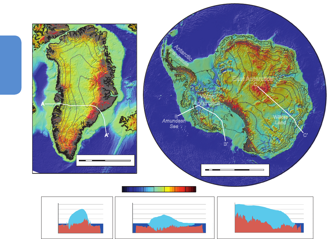
356

Chapter 4 Observations: Cryosphere

Observations suggest that some observed changes in ice shelves and

glaciers on the Antarctic Peninsula are irreversible. These ice bodies

continue to experience rapid and irreversible retreat, coincident with

air temperatures rising at four to six times the global average rate

at some stations (Vaughan et al., 2003), and with warm Circumpolar

Deep Water becoming widespread on the western continental shelf

(Martinson et al., 2008). Collapse of ﬂoating ice shelves on the Ant-

arctic Peninsula, such as the 2002 collapse of the Larsen B Ice Shelf

which is unprecedented in the last 10,000 years, has resulted in speed

up of tributary glaciers by 300 to 800% (De Angelis and Skvarca, 2003;

Rignot et al., 2004; Scambos et al., 2004; Rott et al., 2011). Even if ice-

berg calving was to cease entirely, regrowth of the Larsen B ice shelf to

its pre-collapse state would take centuries based on the ice-shelf speed

and size prior to its collapse (Rignot et al., 2004).

Surface melt that becomes runoff is a major contributor to mass loss

from the Greenland ice sheet, which results in a lower (hence warmer)

ice sheet surface and a lower surface albedo (allowing the surface to

A’

B’

C’

0 1000 2000 (km)

0 1000 (km)

A’

B’

C’

0 500 1000

Scale (km)

Bed elevation (m

)

1500

1000

-1000

-2000

0 500 1000 1500 2000

Scale (km)

4000

2000

-2000

(m)

4000

2000

-2000

(m)

4000

2000

-2000

(m)

East Antarctica

West

Antarctica

Amundsen

Sea

Antarctic

Peninsula

Wilkes

Land

absorb more solar radiation); both processes further increase melt.

The warm summers of the last two decades (van den Broeke et al.,

2009; Hanna et al., 2011), and especially in 2012 (Hall et al., 2013), are

unusual in the multi-centennial record. Exceptionally high melt events

have affected even the far north of Greenland, for example, with the

partial collapse of the ﬂoating ice tongues of Ostenfeld Gletscher and

Zachariae Isstrom in 2000–2006 (Moon and Joughin, 2008).

The importance that subsurface warm waters play in melting the

periphery of ice sheets in Greenland and Antarctica, and the evolution

of these ice sheets, has become much clearer since AR4 (see Sections

4.4.3.1 and 4.4.3.2). New observations in Greenland and Antarctica,

as well as advances in theoretical understanding, show that regions

of ice sheets that are grounded well below sea level are most likely to

experience rapid ice mass loss, especially if the supply of heat to the

ice margin increases (Schoof, 2007; Holland et al., 2008; Joughin and

Alley, 2011; Motyka et al., 2011; Young et al., 2011a; Joughin et al.,

2012; Ross et al., 2012) (See also Figure 4.18.) Where this ice meets the

Figure 4.18 | Subglacial and seabed topography for Greenland and Antarctica derived from digital compilations (Bamber et al., 2013; Fretwell et al., 2013). Blue areas highlight

the marine-based parts of the ice sheets, which are extensive in Antarctica, but in Greenland, relate to speciﬁc glacier troughs. Selected sections through the ice sheet show reverse

bed gradients that exist beneath some glaciers in both ice sheets.

357

Observations: Cryosphere Chapter 4

ocean and does not form an ice shelf, warm waters can increase melt-

ing at the ice front, causing undercutting, higher calving rates, ice-front

retreat (Motyka et al., 2003; Benn et al., 2007; Thomas et al., 2011a)

and consequent speed-up and thinning. Surface runoff also increases

subglacial water discharge at the grounding line, which enhances ice

melting at the ice front (Jenkins, 2011; Xu et al., 2012). Where an ice

shelf is present, ice melt by the ocean may cause thinning of the shelf

as well as migration of the grounding line further inland into deep

basins, with a major impact on buttressing, ﬂow speed and thinning

rate (Thomas et al., 2011a).

The inﬂuence of the ocean on the ice sheets is controlled by the delivery

of heat to the ice sheet margins, particularly to ocean cavities beneath

ice shelves and to calving fronts (Jenkins and Doake, 1991; Jacobs et

al., 2011). The amount of heat delivered is a function of the tempera-

ture and salinity of ocean waters; ocean circulation; and the bathyme-

try of continental shelves, in fjords near glacier fronts and beneath ice

shelves, most of which are not known in sufﬁcient detail (Jenkins and

Jacobs, 2008; Holland et al., 2010; Dinniman et al., 2012; Galton-Fenzi

et al., 2012; Padman et al., 2012). Changes in any of these parameters

would have a direct and rapid impact on melt rates and potentially on

calving ﬂuxes (see Chapter 13).

Ice grounded on a reverse bed-slope, deepening towards the ice sheet

interior, is potentially subject to the marine ice sheet instability (Weert-

man, 1974; Schoof, 2007) (see Box 13.2). Much of the bed of the

West Antarctic Ice Sheet (WAIS) lies below sea level and on a reverse

bed-slope, with basins extending to depths greater than 2 km (Figure

4.18). The marine parts of the WAIS contain ~3.4 m of equivalent sea

level rise (Bamber et al., 2013; Fretwell et al., 2013), and a variety of

evidence strongly suggests that the ice sheet volume has been much

smaller than present in the last 1 million years, during periods with

temperatures similar to those predicted in the next century (see also

Chapter 5) (Kopp et al., 2009). Potentially unstable marine ice sheets

also exist in East Antarctica, for example, in Wilkes Land (Young et al.,

2011a), and these contain more ice than WAIS (9 m sea level equiv-

alent for Wilkes Land). In northern Greenland, ice is also grounded

below sea level, with reverse slopes (Figure 4.18; Joughin et al., 1999).

Observations since AR4 conﬁrm that rapid changes are indeed occur-

ring at the marine margins of ice sheets, and that these changes have

been observed to penetrate hundreds of kilometres inland (Pritchard et

al., 2009; Joughin et al., 2010b).

The Amundsen Sea sector of West Antarctica is grounded signiﬁcantly

below sea level and is the region of Antarctica changing most rapidly at

present. Pine Island Glacier has sped up 73% since 1974 (Rignot, 2008)

and has thinned throughout 1995–2008 at increasing rates (Wingham

et al., 2009) due to grounding line retreat. There is medium conﬁdence

that retreat was caused by the intrusion of warm ocean water into the

sub-ice shelf cavity (Jenkins et al., 2010; Jacobs et al., 2011; Steig et al.,

2012). The neighbouring Thwaites, Smith and Kohler glaciers are also

speeding-up, thinning and contributing to increasing mass loss (Figure

4.14). The present rates of thinning are more than one order of magni-

tude larger than millennial-scale thinning rates in this area (Johnson et

al., 2008). Changes in velocity, elevation, thickness and grounding line

position observed in the past two to three decades in the Pine Island/

Thwaites Glacier sector are not inconsistent with the development of

a marine ice sheet instability triggered by a change in climate forcing,

but neither are they inconsistent solely with a response to external

environmental (probably oceanic) forcing.

In Greenland, there is medium conﬁdence that the recent rapid retreat

of Jakobshavn Isbrae was caused by the intrusion of warm ocean water

beneath the ﬂoating ice tongue (Holland et al., 2008; Motyka et al.,

2011) combined with other factors, such as weakening of the ﬂoat-

ing mixture of sea ice, iceberg debris and blown snow within ice rifts

(Joughin et al., 2008b; Amundson et al., 2010). There is medium con-

ﬁdence that recent variations in southeast Greenland’s glaciers have

been caused by intrusion of warm waters of subtropical origin into

glacial fjords. Since AR4 it has become clear that the mid-2000s speed

up of southeast Greenland glaciers, which caused a doubling of ice

loss from the Greenland ice sheet (Luthcke et al., 2006; Rignot and

Kanagaratnam, 2006; Howat et al., 2008; Wouters et al., 2008), was a

pulse that was followed by a partial slow down (Howat et al., 2008;

Murray et al., 2010). Although changes in elevation in the north are not

as large as in the south, marine sectors were thinning in 2003–2008

(Pritchard et al., 2009; Sorensen et al., 2011).

In contrast to the rapidly changing marine margins of the ice sheets,

land-terminating regions of the Greenland ice sheet are changing more

slowly, and these changes are explained largely by changes in the input

of snow and loss of meltwater (Sole et al., 2011). Surface meltwater,

although abundant on the Greenland ice sheet, does not seem to be

driving signiﬁcant changes in basal lubrication that impact on ice sheet

ﬂow (Joughin et al., 2008b; Selmes et al., 2011; Sundal et al., 2011).

In Greenland, the observed changes are not all irreversible. The Helheim

Glacier in southeast Greenland accelerated, retreated and increased its

calving ﬂux during the period 2002–2005 (Howat et al., 2011; Andre-

sen et al., 2012), but its calving ﬂux similarly increased during the late

1930s – early 1940s (Andresen et al., 2012): an episode from which

the glacier subsequently recovered and re-advanced (Joughin et al.,

2008b). The collapse of the ﬂoating tongue of Jakobshavn Isbrae in

2002 and consequent loss of buttressing has considerably increased

ice ﬂow speeds and discharge from the ice sheet. At present, the gla-

cier grounding line is retreating 0.5–0.6 km yr

–1

(Thomas et al., 2011b;

Rosenau et al., 2013), with speeds in excess of 11 km yr

–1

(Moon et

al., 2012), and the glacier is retreating on a bed that deepens further

inland, which could be conducive to a marine instability. However,

there is evidence that Jakobshavn Isbrae has undergone signiﬁcant

margin changes over the last approximately 8000 years which may

have been both more and less extensive than the recent ones (Young

et al., 2011b).

Since AR4, many new observations indicate that changes in ice sheets

can happen more rapidly than was previously recognised. Similarly,

evidence presented since AR4 indicates that interactions with both the

atmosphere and ocean are key drivers of decadal ice-sheet change. So,

although our understanding of the detailed processes that control the

evolution of ice sheets in a warming climate remains incomplete, there

is no indication in observations of a slowdown in the mass loss from

ice sheets; instead, recent observations suggest an ongoing increase

in mass loss.

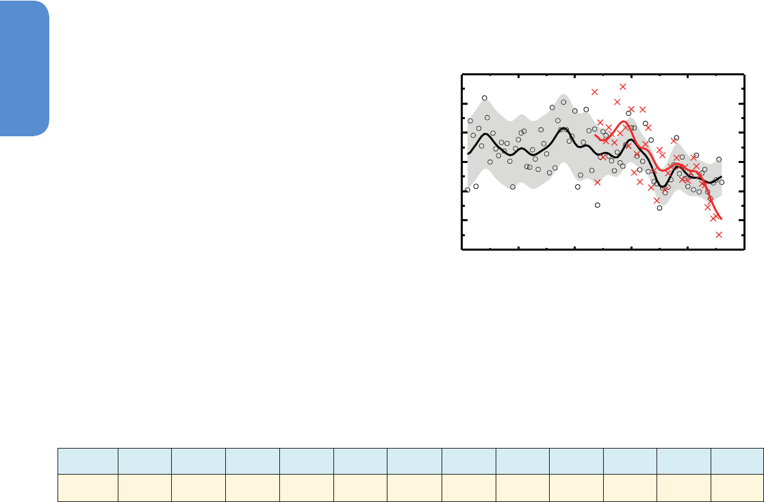
358

Chapter 4 Observations: Cryosphere

4.5 Seasonal Snow

4.5.1 Background

Snowfall is a component of total precipitation and, in that context, is

discussed in Chapter 2 (See Section 2.5.1.3); here we discuss accumu-

lated snow as a climatological indicator. Snow is measured using a

variety of instruments and techniques, and reported using several met-

rics, including snow cover extent (SCE; see Glossary); the seasonal sum

of daily snowfall; snow depth (SD); snow cover duration (SCD), that is,

number of days with snow exceeding a threshold depth; or snow water

equivalent (SWE; see Glossary).

Long-duration, consistent records of snow are rare owing to many

challenges in making accurate and representative measurements.

Although weather stations in snowy inhabited areas often report snow

depth, records of snowfall are often patchy or use techniques that

change over time (e.g., Kunkel et al., 2007). The density of stations and

the choice of metric also varies considerably from country to coun-

try. The longest satellite-based record of SCE is the visible-wavelength

weekly product of the National Oceanic and Atmospheric Administra-

tion (NOAA) dating to 1966 (Robinson et al., 1993), but this covers only

the NH. Satellite mapping of snow depth and SWE has lower accuracy

than SCE, especially in mountainous and heavily forested areas. Meas-

urement challenges are particularly acute in the Southern Hemisphere

(SH), where only about 11 long-duration in situ records continue to

recent times: seven in the central Andes and four in southeast Aus-

tralia. Owing to concerns about quality and duration, global satellite

microwave retrievals of SWE are of less use in the data-rich NH than

in the data-poor SH.

4.5.2 Hemispheric View

By blending in situ and satellite records, Brown and Robinson (2011)

have updated a key indicator of climate change, namely the time series

of NH SCE (Figure 4.19). This time series shows signiﬁcant reductions

over the past 90 years with most of the reductions occurring in the

1980s, and is an improvement over that presented in AR4 in several

ways, not least because the uncertainty estimates are explicitly derived

through the statistical analysis of multiple data sets, which leads to very

high conﬁdence. Snow cover decreases are largest in spring (Table 4.7),

and the rate of decrease increases with latitude in response to larger

albedo feedbacks (Déry and Brown, 2007). Averaged March and April

NH SCE decreased 0.8% [0.5 to 1.1%] per decade over the 1922–2012

period, 1.6% [0.8 to 2.4%] per decade over the 1967–2012 period,

and 2.2% [1.1 to 3.4%] per decade over the 1979–2012 period. In a

new development since AR4, both absolute and relative losses in June

SCE now exceed the losses in March–April SCE: 11.7% [8.8 to 14.6%]

per decade or 53% [40 to 66%] total over the 1967–2012 period and

14.8% [10.3 to 19.3%] per decade over the 1979–2012 period (all

ranges very likely). Note that these percentages differ from those given

by Brown and Robinson (2011) which were calculated relative to the

mean over the 1979–2000 period, rather than relative to the start-

ing point. The loss rate of June SCE exceeds the loss rate for Coupled

Model Intercomparison Project Phase 5 (CMIP5) model projections of

June SCE and also exceeds the well-known loss of September sea ice

extent (Derksen and Brown, 2012). Viewed another way, the NOAA

SCE data indicate that, owing to earlier spring snowmelt, the duration

of the snow season averaged over NH grid points declined by 5.3 days

per decade since winter 1972–1973 (Choi et al., 2010).

Over Eurasia, in situ data show signiﬁcant increases in winter snow

accumulation but a shorter snowmelt season (Bulygina et al., 2009).

From analysis of passive microwave satellite data since 1979, signif-

icant trends toward a shortening of the snowmelt season have been

identiﬁed over much of Eurasia (Takala et al., 2009) and the pan-Arctic

region (Tedesco et al., 2009), with a trend toward earlier melt of about

5 days per decade for the beginning of the melt season, and a trend of

about 10 days per decade later for the end of the melt season.

The correlation between spring temperature and SCE (Figure 4.20)

demonstrates that trends in spring SCE are linked to rising tempera-

ture, and for a well-understood reason: The spring snow cover-albedo

feedback. This feedback contributes substantially to the hemispheric

response to rising greenhouse gases and provides a useful test of global

1920 1940 1960 1980 2000 2020

Year

-6

-4

-2

SCE anomaly (10

)

March-April

June

Annual Jan Feb March April May June July Aug Sep Oct Nov Dec

–0.40* 0.03 –0.13 –0.50* –0.63* –0.90* –1.31* n/a n/a n/a n/a 0.17 0.34

Figure 4.19 | March–April NH snow cover extent (SCE, circles) over the period of

available data, ﬁltered with a 13-term smoother and with shading indicating the 95%

conﬁdence interval; and June SCE (red crosses, from satellite data alone), also ﬁltered

with a 13-term smoother. The width of the smoothed 95% conﬁdence interval is inﬂu-

enced by the interannual variability in SCE. Updated from Brown and Robinson (2011).

For both time series the anomalies are calculated relative to the 1971–2000 mean.

Notes:

*Denotes statistical signiﬁcance at p = 0.05.

Table 4.7 | Least-squares linear trend in Northern Hemisphere snow cover extent (SCE) in 10

per decade for 1967–2012. The equivalent trends for 1922–2012 (available

only for March and April) are –0.19* March and –0.40* April.

359

Observations: Cryosphere Chapter 4

-2 -1 0 1 2

40-60°N Temperature anomaly (°C)

SCE (10

)

Slope -4.5 (% °C

-1

)

Figure 4.20 | Relationship between NH April SCE and corresponding land air tem-

perature anomalies over 40°N to 60°N from the CRUtem4 data set (Jones et al., 2012).

Red circles indicate the years 2000–2012. The correlation is 0.76. Updated from Brown

and Robinson (2011).

snowmelt, or both. However, unravelling the competing effects of

rising temperatures and changing precipitation remains an important

challenge in understanding and interpreting observed changes. Figure

4.21 shows a compilation of many published trends observed at indi-

vidual locations; data were obtained either from tables in the pub-

lished papers, or (when the numerical results in the ﬁgures were not

tabulated) directly from the author, in some cases including updates

to the published data sets. The ﬁgure shows that in most studies, a

majority of sites experienced declines during the varying periods of

record, and where data on site mean temperature or elevation were

available, warmer/lower sites (red circles) were more likely to experi-

ence declines.

Some in situ studies in addition to those in Figure 4.21 deserve discus-

sion. Ma and Qin (2012) described trends by season at 754 stations

aggregated by region in China over 1951–2009; they found statisti-

cally signiﬁcant trends: positive in winter SD in northwest China, and

negative in SD and SWE in spring for China as a whole and spring

SWE for the Qinghai-Xizang (Tibet) Plateau. Marty and Meister (2012)

noted changes at six high-elevation (>2200 m) sites in the European

Alps of Switzerland, Austria, and Germany, consistent with Figure 4.21:

no change in SD in midwinter, shortening of SCD in spring and reduc-

tion in spring SWE and SD coincident with warming. For the Pyrenees,

Lopez-Moreno and Vicente-Serrano (2007) derived proxy SD for 106

sites since 1950 from actual SD measurements since 1985 and weath-

er measurements; they noted declines in spring SD that were related

to changes in atmospheric circulation. In the SH, of seven records in

the Andes, none have signiﬁcant trends in maximum SWE (Masiokas

et al., 2010) over their periods of record. Of four records in Australia

discussed in AR4, all show decreases in spring SWE over their respec-

tive periods of record (Nicholls, 2005), and the only one that has been

updated since the Nicholls (2005) paper shows a statistically signiﬁ-

cant decrease of 37% (Sanchez-Bayo and Green, 2013).

4.5.4 Changes in Snow Albedo

In addition to reductions in snow cover extent, which will reduce the

mean reﬂectivity of particular regions, the reﬂectivity (albedo) of the

snow itself may also be changing in response to human activities.

Unfortunately, there are extremely limited data on the changes of

albedo over time, and we must rely instead on analyses from ice cores,

direct recent observations, and modelling. Flanner et al. (2007), using a

detailed snow radiative model coupled to a global climate model and

estimates of biomass burning, estimated that the human-induced radi-

ative forcing by deposition of black carbon on snow cover is +0.054

(0.007–0.13) W m

–2

globally, of which 80% is from fossil fuels. How-

ever, spatially comprehensive surveys of impurities in Arctic snow in

the late 2000s and mid-1980s suggested that impurities decreased

between those two periods (Doherty et al., 2010) and hence albedo

changes have probably not made a signiﬁcant contribution to recent

reductions in Arctic ice and snow.

climate models (Fernandes et al., 2009) (see also Chapter 9). Indeed,

the observed declines in land snow cover and sea ice have contributed

roughly the same amount to changes in the surface energy ﬂuxes, and

the albedo feedback of the NH cryosphere is likely in the range 0.3 to

1.1 W m

–2

–1

(Flanner et al., 2011). Brown et al. (2010) used satellite,

reanalyses and in situ observations to document variability and trend

in Arctic spring (May–June) SCE over the 1967–2008 period. In June,

with Arctic albedo feedback at a maximum, SCE decreased 46% (as of

2012, now 53%) and air temperature explains 56% of the variability.

For the SH, as noted above (see Section 4.5.1), there are no corre-

spondingly long visible-wavelength satellite records, but microwave

data date from 1979. Foster et al. (2009) presented the ﬁrst satel-

lite study of variability and trends in any measure of snow for South

America, in this case SWE from microwave data. They focused on the

May-September period and noted large year-to-year variability and

some lower frequency variability—the July with most extensive snow

cover had almost six times as much as the July with the least extensive

snow cover—but identiﬁed no trends.

4.5.3 Trends from In Situ Measurements

AR4 stimulated a review paper (Brown and Mote, 2009) that synthe-

sized modelling results as well as observations from many countries.

They showed that decreases in various metrics of snow are most likely

to be observed in spring and at locations where air temperatures

are close to the freezing point, because changes in air temperature

there are most effective at reducing snow accumulation, increasing

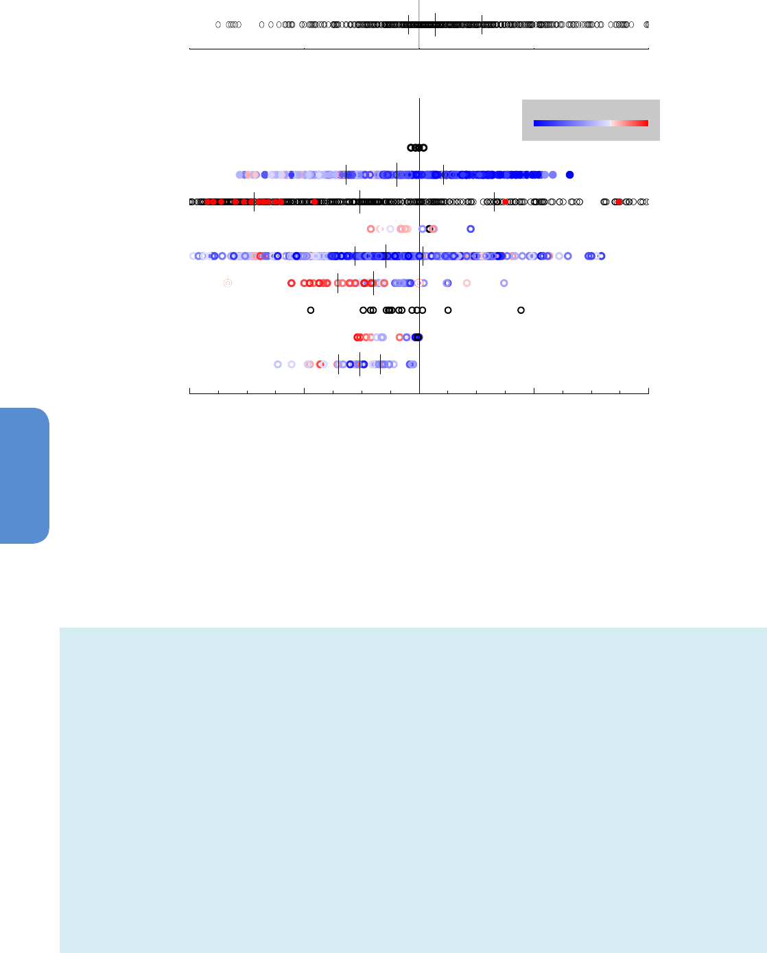
360

Chapter 4 Observations: Cryosphere

-2 -1 0 1 2

# days per year

9a. 31%

-2 -1 0 1 2

% per year

-10

C -5

C 0

C 5

high elev low elev

b: 50%

c: 60%

59 71

d: 65%

e: 66%

f: 72%

g: 73%

h: 80%

i: 100%

j: 100%

Figure 4.21 | Compilation of studies (rows) showing trends at individual stations (symbols in each row, with percentage of trends that are negative) showing that most sites

studied show decreases in snow, especially at lower and/or warmer locations. For each study, if more than one quantity was presented, only the one representing spring conditions

is shown. (a) Number of days per year with SD >20 cm at 675 sites in northern Eurasia, 1966–2010 (Bulygina et al., 2011). (b) March–April–May snowfall for 500 stations in

California, aggregated into four regions (Christy, 2012). (c) maximum SWE at 393 sites in Norway, 1961–2009 (Skaugen et al., 2012); statistically signiﬁcant trends are denoted

by solid circles. (d) SD at 560 sites in China, 1957–2012 (Ma and Qin, 2012); statistically signiﬁcant trends are denoted by solid red circles. (e) Snow cover duration at 15 sites in

the Romanian Carpathians, 1961–2003 (Micu, 2009). (f) 1 April SWE at 799 sites, 1950–2000, in western North America (Mote, 2006). (g) Difference between 1990s and 1960s

March SD at 89 sites in Japan (Ishizaka, 2004). (h) SCD at 15 sites for starting years near 1931, ending 2000 (Petkova et al., 2004). (i) SCD at 18 sites in Italy, 1950–2009 (Valt

and Cianfarra, 2010). (j) SCD at 34 sites in Switzerland, 1948–2007, from Marty (2008). See text for deﬁnitions of abbreviations. For (b) through ( j), the quantity plotted is the

percentage change of a linear ﬁt divided by the number of years of the ﬁt. For studies with more than 50 sites, the median, upper and lower quartiles are shown with vertical lines.

In a few cases, some trends lie beyond the edges of the graph; these are indicated by a numeral at the corresponding edge of the graph, for example, two sites >2% yr–1 in row (f).

Colours indicate temperature or, for studies e) and i), elevation using the lowest and highest site in the respective data set to set the colour scale. Note the prevalence of negative

trends at lower/warmer sites.

Box 4.1 | Interactions of Snow within the Cryosphere

Snow is just one component of the cryosphere, but snow also sustains ice sheets and glaciers, and has strong interactions with all the

other cryospheric components, except sub-sea permafrost. For example, snow can affect the rate of sea-ice production, and can alter

frozen ground through its insulating effect. Snowfall and the persistence of snow cover are strongly dependent on atmospheric tem-

perature and precipitation, and are thus likely to change in complex ways in a changing climate (e.g, Brown and Mote, 2009).

For the Earth’s climate in general, and more speciﬁcally, the cryospheric components on which snow falls, the two most important

physical properties of snow are its high albedo (reﬂectivity of solar radiation) and its low thermal conductivity, which results because

its high air content makes it an excellent thermal insulator. Both factors substantially alter the ﬂux of energy between the atmosphere

and the material beneath the snow cover. Snow also has a major impact on the total energy balance of the Earth’s surface because

large regions in the NH are seasonally covered by snow (e.g., Barry and Gran, 2011). When seasonal snow melts it is also an important

fresh water resource.

The high albedo of snow has a strong impact on the radiative energy balance of all surfaces on which it lies, most of which (including

glaciers and sea ice) are much less reﬂective. For example, the albedo of bare glacier or sea ice is typically only 20 to 30%, and hence

(continued on next page)

361

Observations: Cryosphere Chapter 4

Box 4.1 (continued)

70 to 80% of solar radiation is absorbed at the surface. For ice at the melting point, this energy melts the ice. With a fresh snow cover

over ice, the albedo changes to 80% or even higher and melting is greatly reduced (e.g., Oerlemans, 2001). The effect is similar for

other land surfaces—bare soil, frozen ground, low-lying vegetation—but here the thermal properties of the snow cover also play an

important role by insulating the ground from changes in ambient air temperature.

While an insulating snow cover can reduce the growth of sea ice, a heavy snow load, particularly in the Antarctic, often depresses the

sea ice surface below sea level and this leads to faster transformation of snow to ice (see FAQ 4.1). Even without ﬂooding, the basal

snow layer on Antarctic sea ice tends to be moist and saline because brine is wicked up through the snow cover. In regions of heavily

ridged and deformed sea ice, snow redistributed by wind smoothes the ice surface, reducing the drag of the air on the ice and thus

slowing ice drift and reducing heat exchange (Massom et al., 2001) .

For frozen ground, the insulation characteristics of snow cover are particularly important. If the air above is colder than the material

on which it lies, the presence of snow will reduce heat transfer upwards, especially for fresh snow with a low density. This could, for

example, reduce the seasonal freezing of soil, slow down the freezing of the active layer (seasonally thawed layer) or protect permafrost

from cooling. Alternatively, if the air is warmer than the material beneath the snow, heat transfer downwards from the air is reduced

and the presence of snow cover can increase the thickness of seasonal soil freeze and protect permafrost from warming. Which process

applies depends on the timing of the snowfall, its thickness, and its duration (e.g., Zhang, 2005; Smith et al., 2012).

For the preceding reasons, the timing of snowfall and the persistence of snow cover are of major importance. Whereas snow falling on

glaciers and ice sheets in summer has a strongly positive (sustaining) effect on the mass budget, early snow cover can reduce radiative

and conductive cooling and freezing of the active layer. During winter, snowfall is the most important source of nourishment for most

glaciers, but radiative cooling of frozen ground is strongly reduced by thick snow cover (Zhang, 2005).

4.6 Lake and River Ice

The assessment of changes in lake and river ice is made more difﬁcult

by several factors. Until the satellite era, some nations collected data

from numerous lakes and rivers and others none; many published stud-

ies focus on a single lake or river. Many records have been discontinued

(Prowse et al., 2011), and consistency of observational methods is a

challenge, especially for date of ice break-up of ice on rivers when the

process of break-up can take as long as 3 months (Beltaos and Prowse,

2009).

The most comprehensive description is the analysis of 75 lakes, mostly

in Scandinavia and the northern USA, but with one each in Switzerland

and Russia (Benson et al., 2012). Examining 150-, 100-, and 30-year

periods ending in spring 2005, they found the most rapid changes in

the most recent 30-year period (medium conﬁdence) with trends in

freeze-up 1.6 days per decade later and breakup 1.9 days per decade

earlier. Wang et al. (2012) found a total ice cover reduction on the north

American Great Lakes of 71% over the 1973–2010 period of record,

using weekly ice charts derived from satellite observations (medium

conﬁdence). Jensen et al. (2007) examined data from 65 water bodies

in the Great Lakes region between Minnesota and New York (not

including the Great Lakes themselves) and found trends in freeze-up

3.3 days per decade later, trends in breakup 2.1 days per decade ear-

lier, and rates of change over 1975–2004 that were bigger than those

over 1846–1995. Spatial patterns in trends are ambiguous: Latifovic

and Pouliot (2007) found larger trends in higher latitudes over Canada,

but Hodgkins et al. (2002) found larger trends in lower latitudes in the

northeastern USA.

In the only reported study since the 1990s of ice on SH lakes, Green

(2011) suggested on the basis of available evidence that break-up of

ice cover on Blue Lake in the Snowy Mountains of Australia had shifted

from November to October between observation periods 1970–1972

and 1998–2010.

Several studies made quantitative connections between ice cover and

temperature. For instance, Benson et al. (2012) found signiﬁcant corre-

lations between mean ice duration and mean NH land air temperature

in fall-winter-spring (r

= 0.48) and between spring air temperature

and breakup (r

= 0.36); see also the review by Prowse et al. (2011).

Studies of changes in river ice have used both disparate data and time

intervals, ranging in duration from multi-decade to more than two cen-

turies, and most focus on a single river. Beltaos and Prowse (2009),

summarizing most available information for northern rivers, noted an

almost universal trend towards earlier break-up dates but considerable

spatial variability in those for freeze-up, and noted too that changes

were often more pronounced during the last few decades of the 20th

century. They noted that the 20th century increase in mean air tem-

perature in spring and autumn has produced in many areas a change

of about 10 to 15 days toward earlier break-up and later freeze-up,

although the relationship with air temperatures is complicated by the

roles of snow accumulation and spring runoff.

In summary, the limited evidence available for freshwater (lake and

river) ice indicates that ice duration is decreasing and average sea-

sonal ice cover shrinking (low conﬁdence), and the following general

patterns (each of which has exceptions): rates of change in timing are

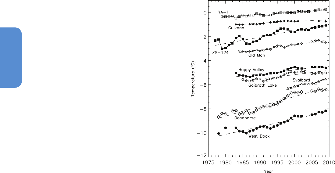
362

Chapter 4 Observations: Cryosphere

generally, but not universally, (1) higher for spring breakup than fall

freeze-up; (2) higher for more recent periods; (3) higher at higher eleva-

tions (Jensen et al., 2007) and (4) quantitatively related to temperature

changes.

4.7 Frozen Ground

4.7.1 Background

Frozen ground occurs across the world at high latitudes, in mountain

regions, beneath glacial ice and beneath lakes and seas. It is a product

of cold weather and climate, and can be diurnal, seasonal or peren-

nial. Wherever the ground remains at or below 0°C for at least two

consecutive years, it is called permafrost (Van Everdingen, 1998), and

this too can occur beneath the land surface (terrestrial permafrost) and

beneath the seaﬂoor (subsea permafrost). In this chapter, the term

permafrost refers to terrestrial permafrost unless specified.

Both the temperature and extent of permafrost are highly sensitive

to climate change, but the responses may be complex and highly het-

erogeneous (e.g., Osterkamp, 2007). Similarly, the annual freezing

and thawing of seasonally frozen ground is coupled to the land sur-

face energy and moisture ﬂuxes, and thus to climate. Since, perma-

frost and seasonally frozen ground, can contain signiﬁcant fractions

of ice, changes in landscapes, ecosystems and hydrological processes

can occur when it forms or degrades (Jorgenson et al., 2006; Gruber

and Haeberli, 2007; White et al., 2007). Furthermore, frozen organic

soils contain considerable quantities of carbon, more than twice the

amount currently in the atmosphere (Tarnocai et al., 2009), and perma-

frost thawing exposes previously frozen carbon to microbial degrada-

tion and releases radiatively active gases, such as carbon dioxide (CO

)

and methane (CH

), into the atmosphere (Zimov et al., 2006; Schuur et

al., 2009; Schaefer et al., 2011) (for a detailed assessment of this issue,

see Chapter 6). Similarly, recent evidence suggests that degradation of

permafrost may also permit the release of nitrous oxide (N

O), which

is also radiatively active (Repo et al., 2009; Marushchak et al., 2011).

Finally, permafrost degradation may directly affect the lives of people,

both in northern and high-mountain areas, through impacts on the

landscape, vegetation and infrastructure (WGII, Chapter 28).

4.7.2 Changes in Permafrost

4.7.2.1 Permafrost Temperature

The ice content and temperature of permafrost are the key parame-

ters that determine its physical state. Permafrost temperature is a key

parameter used to document changes to permafrost. Permafrost tem-

perature measured at a depth where seasonal variations cease to occur

is generally used as an indicator of long-term change and to represent

the mean annual ground temperature (Romanovsky et al., 2010a). For

most sites this depth occurs in the upper 20 m.

In the SH, permafrost temperatures as low as –23.6°C have been

observed in the Antarctic (Vieira et al., 2010), but in the NH, permafrost

temperatures generally range from –15°C to close to the freezing point

(Figure 4.22) (Romanovsky et al., 2010a). They are usually coldest in

high Arctic regions and gradually increase southwards, but substantial

differences do occur at the same latitude. For example, as a result of

the proximity to warm ocean currents, the southern limit of permafrost

is farther north, and permafrost temperature is higher in Scandinavia

and north-western Russia than it is in Arctic regions of Siberia and

North America (Romanovsky et al., 2010a).

In Russia, permafrost temperature measurements reach back to the

early 1930s (Romanovsky et al., 2010b), in North America to the late

1940s (Brewer, 1958) and in China to the early 1960s (Zhou et al.,

2000; Zhao et al., 2010). Systematic measurements, however, began

mostly in the late 1970s and early 1980s (Zhou et al., 2000; Oster-

kamp, 2007; Smith et al., 2010). In addition, since the AR4, consider-

able effort (especially during the International Polar Year) has gone

into enhancing the observation network and establishing a base-

line against which future changes in permafrost can be measured

(Romanovsky et al., 2010a). However, it should be noted that there

still exist comparatively few measurements of permafrost tempera-

ture in the SH (Vieira et al., 2010).

Figure 4.22 | Time series of mean annual ground temperatures at depths between

10 and 20 m for boreholes throughout the circumpolar northern permafrost regions

(Romanovsky et al., 2010a). Data sources are from Romanovsky et al. (2010b) and

Christiansen et al. (2010). Measurement depth is 10 m for Russian boreholes, 15 m

for Gulkana and Oldman, and 20 m for all other boreholes. Borehole locations are:

ZS-124, 67.48°N 063.48°E; 85-8A, 61.68°N 121.18°W; Gulkana, 62.28°N 145.58°W;

YA-1, 67.58°N 648°E; Oldman, 66.48°N 150.68°W; Happy Valley, 69.18°N 148.88°W;

Svalbard, 78.28°N 016.58°E; Deadhorse, 70.28°N 148.58°W and West Dock, 70.48°N

148.58°W. The rate of change (degrees Celsius per decade) in permafrost temperature

over the period of each site record is: ZS-124: 0.53 ± 0.07; YA-1: 0.21 ± 0.02; West

Dock: 0.64 ± 0.08; Deadhorse: 0.82 ± 0.07; Happy Valley:0.34 ± 0.05; Gaibrath Lake:

0.35 ± 0.07; Gulkana:0.15 ± 0.03; Old Man: 0.40 ± 0.04 and Svalvard: 0.63 ± 0.09.

(The trends are very likely range, 90%.)

363

Observations: Cryosphere Chapter 4

In most regions, and at most sites, permafrost temperatures have

increased during the past three decades (high conﬁdence): at rather

fewer sites, permafrost temperatures show little change, or a slight

decrease (Figure 4.22; Table 4.8). However, it is important to discrim-

inate between cold permafrost, with mean annual ground tempera-

tures below –2°C, and warm permafrost at temperatures above –2°C

(Cheng and Wu, 2007; Smith et al., 2010; Wu and Zhang, 2010). Warm

permafrost is found mostly in the discontinuous permafrost zone,

while cold permafrost exists in the continuous permafrost zone and

only occasionally in the discontinuous permafrost zone (Romanovsky

et al., 2010a).

Overall, permafrost temperature increases are greater in cold

permafrost than they are in warm permafrost (high conﬁdence). This

is especially true for warm ice-rich permafrost, due to heat absorbed

by partial melting of interstitial ice, slowing and attenuating temper-

ature change (Romanovsky et al., 2010a). The temperatures of cold

permafrost across a range of regions have increased by up to 2°C since

the 1970s (Table 4.8 and Callaghan et al., 2011); however, the timing of

warming events has shown considerable spatial variability (Romano-

vsky et al., 2010a).

Temperatures of warm permafrost have also increased over the last

three decades, but generally by less than 1°C. Warm permafrost is

Region

Permafrost

Temperature

During IPY (°C)

Permafrost

Temperature

Change (°C)

Depth

(m)

Period of Record Source

North America

Northern Alaska –5.0 to –10.0 0.6–3 10–20 Early 1980s–2009 Osterkamp (2005, 2007); Smith et al.

(2010); Romanovsky et al. (2010a)

Mackenzie Delta and Beau-

fort coastal region

–0.5 to –8.0 1.0–2.0 12–20 Late 1960s–2009 Burn and Kokelj (2009); Burn and Zhang

(2009); Smith et al. (2010)

Canadian High Arctic –11.8 to –14.3 1.2–1.7 12–15 1978–2008 Smith et al. (2010, 2012)

Interior of Alaska, 0.0 to –5.0 0.0–0.8 15–20 1985–2009 Osterkamp (2008); Smith et al. (2010);

Romanovsky et al. (2010a)

Central and Southern Mackenzie Valley >–2.2 0.0–0.5 10–12 1984–2008 Smith et al. (2010)

Northern Quebec >–5.6 0.0–1.8 12–20 1993–2008 Allard et al. (1995); Smith et al. (2010)

Europe

European Alps >–3 0.0–0.4 15–20 1990s–2010 Haeberli et al. (2010); Noetzli and Vonder

Muehll (2010); Christiansen et al. (2012)

Russian European North –0.1 to –4.1 0.3–2.0 8–22 1971–2010 Malkova (2008); Oberman (2008); Romanovsky

et al. (2010b); Oberman (2012)

Nordic Countries –0.1 to –5.6 0.0–1.0 2–15 1999–2009 Christiansen et al. (2010); Isaksen et al. (2011)

Northern and Central Asia

Northern Yakutia –4.3 to –10.8 0.5–1.5 14–25 early 1950s–2009 Romanovsky et al. (2010b)

Trans-Baykal region –4.7 to –5.1 0.5–0.8 19–20 late 1980s–2009 Romanovsky et al. (2010b)

Qinghai-Xizang Plateau –0.2 to –3.4 0.2–0.7 6 1996–2010 Cheng and Wu (2007); Li et al. (2008); Wu

and Zhang (2008); Zhao et al. (2010)

Tian Shan –0.4 to –1.1 0.3–0.9 10–25 1974–2009 (Marchenko et al. (2007); Zhao et al. (2010)

Mongolia 0.0 to <–2.0 0.2–0.6 10–15 1970–2009 Sharkhuu et al. (2007); Zhao et al.

(2010); Ishikawa et al. (2012)

Others

Maritime Antarctica –0.5 to –3.1 NA 20–25 2007–2009 Vieira et al. (2010)

Continental Antarctica –13.9 to –19.1 NA 20–30 2005–2008 Vieira et al. (2010); Guglielmin et al. (2011)

East Greenland –8.1 NA 3.25 2008–2009 Christiansen et al. (2010)

sometimes nearly isothermal with depth; as is observed in mountain

regions such as the European Alps (Noetzli and Vonder Muehll, 2010),

Scandinavia (Christiansen et al., 2010), the Western Cordillera of North

America (Smith et al., 2010; Lewkowicz et al., 2011), the Qinghai-Xi-

zang (Tibet) Plateau (Zhao et al., 2010; Wu et al., 2012) and in the

northern high latitudes in the southern margins of discontinuous per-

mafrost regions (Romanovsky et al., 2010b; Smith et al., 2010). In such

areas, permafrost temperatures have shown little or no change, indi-

cating that permafrost is thawing internally but remaining very close

to the melting point (Smith et al., 2010). Cooling of permafrost due to

atmospheric temperature ﬂuctuations has been observed; for exam-

ple, in the eastern Canadian Arctic until the mid-1990s (Smith et al.,

2010); but some examples have been short-lived and others controlled

by site-speciﬁc conditions (Marchenko et al., 2007; Wu and Zhang,

2008; Noetzli and Vonder Muehll, 2010; Zhao et al., 2010). In at least

one case in the Antarctic, permafrost warming has been observed in a

region with almost stable air temperatures (Guglielmin and Cannone,

2012).

Permafrost warming is mainly in response to increased air temperature

and changing snow cover (see Box 4.1). In cold permafrost regions,

especially in tundra regions with low ice content (such as bedrock)

where permafrost warming rates have been greatest, changes in snow

cover may play an important role (Zhang, 2005; Smith et al., 2010).

Table 4.8 | Permafrost temperatures during the International Polar Year (2007–2009) and their recent changes. Each line may refer to one or more measurements sites.

364

Chapter 4 Observations: Cryosphere

In forested areas, especially in warm ice-rich permafrost, changes

in permafrost temperature are reduced by the effects of the surface

insulation (Smith et al., 2012; Throop et al., 2012) and latent heat

(Romanovsky et al., 2010a).

4.7.2.2 Permafrost Degradation

Permafrost degradation refers to a decrease in thickness and/or areal

extent. In particular, the degradation can be manifested by a deepen-

ing of summer thaw, or top-down or bottom-up permafrost thawing,

and a development of taliks (see Glossary). Other manifestations of

degradation include geomorphologic changes such as the formation of

thermokarst terrain (see Glossary and Jorgenson et al., 2006), expan-

sion of thaw lakes (Sannel and Kuhry, 2011) active-layer detachment

slides along slopes, rock falls (Ravanel et al., 2010), and destabilized

rock glaciers (Kääb et al., 1997; Haeberli et al., 2006; Haeberli et al.,

2010). Although most permafrost has been degrading since the Little

Ice Age (Halsey et al., 1995), the trend was relatively modest until the

past two decades, during which the rate of degradation has increased

in some regions (Romanovsky et al., 2010b).

Signiﬁcant permafrost degradation has been reported in the Russian

European North (medium conﬁdence). Warm permafrost with a thick-

ness of 10 to 15 m thawed completely in the period 1975–2005 in

the Vorkuta area (Oberman, 2008). And although boundaries between

permafrost types are not easy to map, the southern permafrost bound-

ary in this region is reported to have moved north by about 80 km and

the boundary of continuous permafrost has moved north by 15 to 50

km (Oberman, 2008) (medium conﬁdence). Taliks have also developed

in relatively thick permafrost during the past several decades. In the

Vorkuta region, the thickness of existing closed taliks increased by 0.6

to 6.7 m over the past 30 years (Romanovsky et al., 2010b). Permafrost

thawing and talik formation has occurred in the Nadym and Urengoy

regions in north- western Russian (Drozdov et al., 2010). Long-term

permafrost thawing has been reported around the city of Yakutsk, but

this in this case, the thawing may have been caused mainly by forest

ﬁres or human disturbance (Fedorov and Konstantinov, 2008). Perma-

frost degradation has also been reported on the Qinghai-Xizang (Tibet)

Plateau (Cheng and Wu, 2007; Li et al., 2008).

Coastal erosion and permafrost degradation appear to be evident

along many Arctic coasts in recent years, with complex interactions

between them (Jones et al., 2009). In part, these interactions arise

from the thermal and chemical impact of sea water on cold terrestrial

permafrost (Rachold et al., 2007). Similar impacts arise for permafrost

beneath new thaw lakes, which have been formed in recent years (e.g.,

Sannel and Kuhry, 2011). In northern Alaska, estimates of permafrost

thawing under thaw lakes are in the range 0.9 to 1.7 cm a

–1

(Ling and

Zhang, 2003).

Since AR4, destabilized rock glaciers have received increased attention

from researchers. A rock glacier is a mass of perennially frozen rock

fragments on a slope, that contains ice in one or more forms and shows

evidence of past or present movement (Van Everdingen, 1998; Haeberli

et al., 2006). Time series acquired over recent decades by terrestrial

surveys indicate acceleration of some rock glaciers as well as seasonal

velocity changes related to ground temperatures (Bodin et al., 2009;

Noetzli and Vonder Muehll, 2010; Schoeneich et al., 2010; Delaloye et

al., 2011). Similarly, photo-comparison and photogrammetry have indi-

cated collapse-like features on some rock glaciers (Roer et al., 2008).

The clear relationship between mean annual air temperature at the

rock glacier front and rock glacier velocity points to a likely temper-

ature inﬂuence and a plausible causal connection to climate (Kaab et

al., 2007). Strong surface lowering of rock glaciers has been reported in

the Andes (Bodin et al., 2010), indicating melting of ground ice in rock

glaciers and permafrost degradation.

4.7.3 Subsea Permafrost

Subsea permafrost is similar to its terrestrial counterpart, but lies

beneath the coastal seas. And as with terrestrial permafrost, subsea

permafrost is a substantial reservoir and/or a conﬁning layer for gas

hydrates (Koch et al., 2009). It is roughly estimated that subsea perma-

frost contains 2 to 65 Pg of CH

hydrate (McGuire et al., 2009). Obser-

vations of gas release on the East Siberian Shelf and high methane

concentrations in water-column and air above (Shakhova et al., 2010a,

2010b) have led to the suggestion that permafrost thawing creates

pathways for gas release.

Subsea permafrost in the Arctic is generally relict terrestrial perma-

frost (Vigdorchik, 1980), inundated after the last glaciation and now

degrading under the overlying shelf sea. Permafrost may, however, also

form when the sea is shallow, permitting sediment freezing through

bottom-fast winter sea ice (Solomon et al., 2008; Stevens et al., 2010).

A 76-year record of bottom water temperature in the Laptev Sea (Dmi-

trenko et al., 2011) showed warming of 2.1°C since 1985 in the near-

shore zone (<10 m water depth), as lengthening summers reduced

sea ice extent and increased solar heating. Degradation rates of the

ice-bearing permafrost following inundation have been estimated to

be 1 to 20 cm a

–1

on the East Siberian Shelf (Overduin et al., 2007) and

1 to 4 cm a

–1

in the Alaskan Beaufort Sea (Overduin et al., 2012).

4.7.4 Changes in Seasonally Frozen Ground

Seasonally frozen ground is a soil layer that freezes and thaws annu-

ally, which may or may not overlie terrestrial permafrost, and also

includes some portions of the Arctic seabed that freeze in winter. A key

parameter regarding seasonally frozen ground overlying permafrost

is the active-layer thickness (ALT; see Glossary), which indicates the

depth of the seasonal freeze–thaw cycle, and which is dependent on

climate and other factors; for example, vegetation cover (Smith et al.,

2009). Many observations across many regions have revealed trends in

the thickness of the active laver (high conﬁdence).

4.7.4.1 Changes in Active-Layer Thickness

Many observations have revealed a general positive trend in the thick-

ness of the active layer (see Glossary) for discontinuous permafrost

regions at high latitudes (medium conﬁdence). Based on measurements

from the International Permafrost Association (IPA) Circumpolar Active

Layer Monitoring (CALM) programme, active-layer thickening has been

observed since the 1970s and has accelerated since 1995 in north-

ern Europe (Akerman and Johansson, 2008; Callaghan et al., 2010),

and on Svalbard and Greenland since the late-1990s (Christiansen et

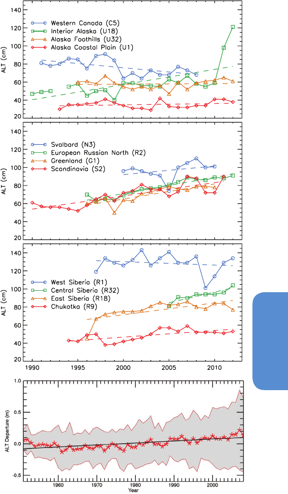
365

Observations: Cryosphere Chapter 4

d) Composite ALT from RHM station

a) Northern America

b) European North

c) Northern Asia

al., 2010). The ALT has increased signiﬁcantly in the Russian European

North (Mazhitova, 2008), East Siberia (Fyodorov-Davydov et al., 2008),

and Chukotka (Zamolodchikov, 2008) since the mid-1990s. Burn and

Kokelj (2009) found, for a site in the Mackenzie Delta area, that ALT

increased by 8 cm between 1983 and 2008, although the record does

exhibit high interannual variability as has been observed at other sites

in the region (Smith et al., 2009). ALT has increased since the mid-

1990s in the eastern portion of the Canadian Arctic, with the largest

increase occurring at bedrock sites in the discontinuous permafrost

zone (Smith et al., 2010).

The interannual variations and trends of the active-layer thickness in

Northern America, Northern Europe and Northern Asia from 1990 to

2012 are presented in Figure 4.23. Large regional variations in the

yearly variability patterns and trends are apparent. While increases in

ALT are occurring in the Eastern Canadian Region (Smith et al., 2009),

a slightly declining trend is observed in the Western Canadian Region

(Figure 4.23a). In Northern Europe, the trends in the study areas are

similar and consistently positive (Figure 4.23b). On the other hand, in

Northern Asia, trends are generally strongly positive with the excep-

tion of West Siberia, where the trend is slightly negative (Figure 4.23c).

On the interior of Alaska, slightly increasing ALT from 1990 to 2010

was followed by anomalous increases in 2011 and in 2012. Overall,

a general increase in ALT since the 1990s has been observed at many

stations in many regions (medium conﬁdence). The general increase

is shown in Figure 4.23d, which shows the results of analysis of data

from about 44 stations in Russia indicating a change of almost 0.2 m

from 1950 to 2008.

At some measurement sites on the Qinghai-Xizang (Tibet) Plateau, ALT

was reported to be increasing at 7.8 cm yr

–1

over a period from 1995

through 2010 (Wu and Zhang, 2010). The high rates may have been the

result of local disturbances since more recent studies indicate rates of

1.33 cm yr

–1

for the period 1981–2010 and 3.6 cm yr

–1

for the period

1998–2010 (e.g., Zhao et al., 2010; Li et al., 2012a).

During the past decade, increases in ALT up to 4.0 cm yr

–1

were

observed in Mongolian sites characterized as a warm permafrost region

(Sharkhuu et al., 2007). Changes in ALT were also detected in Tian Shan

(Marchenko et al., 2007; Zhao et al., 2010), and in the European Alps,

where increases in ALT were largest during years of hot summers but

a strong dependence on surface and subsurface characteristics was

noted (Noetzli and Vonder Muehll, 2010).

In several areas, across North America and in West Siberia, large-inter

annual variations obscure any trends in ALT (high conﬁdence, Figure

4.23). No trend in ALT was observed on the Alaskan North Slope from

1993 to 2010 (Streletskiy et al., 2008; Shiklomanov et al., 2010) and

also in the Mackenzie Valley (Smith et al., 2009) and in West Siberia

(Vasiliev et al., 2008) since the mid-1990s (Figure 4.23). At some sites,

such as at Western Canada (C5) and Western Siberia (R1) (Figure 4.23),

the active layer thickness was actually decreasing.

The penetration of thaw into ice-rich permafrost at the base of the

active layer is often accompanied by loss of volume due to consolida-

tion. At several sites, this has been shown to cause surface subsidence

(medium conﬁdence). Results from ground-based measurements at

Figure 4.23 | Active layer thickness from different locations for slightly different peri-

ods between 1990 and 2012 in (a) Northern America, (b) Northern Europe, and (c)

Northern Asia. The dashed lines represents linear ﬁt to each set of data. ALT data for

Northern America, Northern Asia and Northern Europe were obtained from the Inter-

national Permafrost Association (IPA) CALM website (http://www.udel.edu/Geography/

calm/about/permafrost.html). The number of Russian Hydrometeorological Stations

(RHM) stations has expanded from 31 stations as reported from Frauenfeld et al. (2004)

and Zhang et al. (2005) to 44 stations and the time series has extended from 1990 to

2008. (d) Departures from the mean of active layer thickness in Siberia from 1950 to

2008. The red asterisk represents the mean composite value, the shaded area indicates

the standard deviation and the black line is the trend. Data for Siberia stations were

obtained from the Russian Hydrometeorological Stations (RHM).

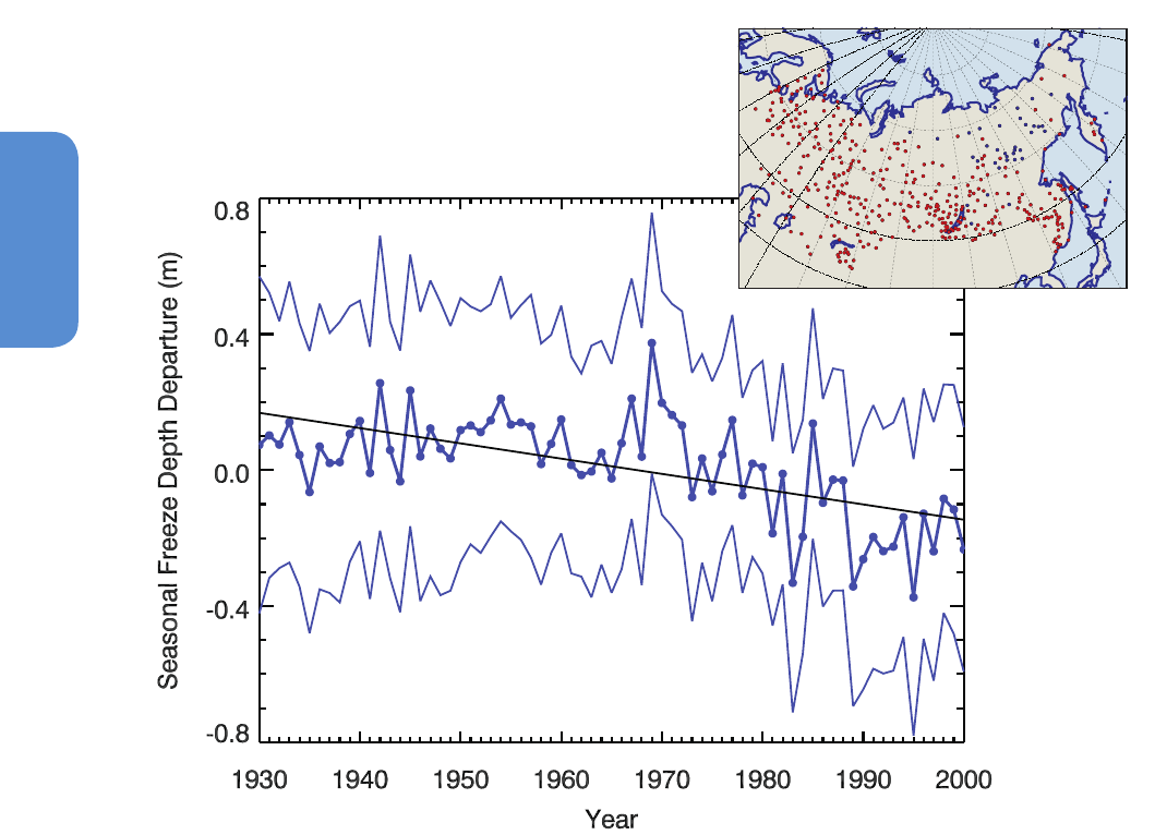
366

Chapter 4 Observations: Cryosphere

selected sites on the North Slope of Alaska indicate 11 to 13 cm in sur-

face subsidence over the period 2001–2006 (Streletskiy et al., 2008), 4

to 10 cm from 2003 to 2005 in the Brooks Range (Overduin and Kane,

2006) and up to 20 cm in the Russian European North (Mazhitova and

Kaverin, 2007). Subsidence has also been identiﬁed using space-borne

interferometric synthetic aperture radar (InSAR) data. Surface defor-

mation was detected using InSAR over permafrost on the North Slope

of Alaska during the 1992–2000 thaw seasons and a long-term surface

subsidence of 1 to 4 cm per decade (Liu et al., 2010). Such subsidence

could explain why in situ measurements at some locations reveal neg-

ligible trends in ALT changes during the past two decades, despite the

fact that atmospheric and permafrost temperatures increased during

that time.

4.7.4.2 Changes in Seasonally Frozen Ground in Areas Not

Underlain by Permafrost

An estimate based on monthly mean soil temperatures from 387 sta-

tions across part of the Eurasian continent suggested that the thickness

Figure 4.24 | Annual anomalies of the average thickness of seasonally frozen depth in Russia from 1930 to 2000. Each data point represents a composite from 320 stations as

compiled at the Russian Hydrometeorological Stations (RHM) (upper right inset). The composite was produced by taking the sum of the thickness measurements from each station

and dividing the result by the number of stations operating in that year. Although the total number of stations is 320, the number providing data may be different for each year but

the minimum was 240. The yearly anomaly was calculated by subtracting the 1971–2000 mean from the composite for each year. The thin lines indicate the 1 standard deviation

(1σ) (likely) uncertainty range. The line shows a negative trend of –4.5 cm per decade or a total decrease in the thickness of seasonally frozen ground of 31.9 cm from 1930 to

2000 (Frauenfeld and Zhang, 2011).

120

150

180

170 E

160 E

170 W

140 E

130 E

110 E

100 E

80 E

70 E

50 E

40 E

20 E

10 E

of seasonally frozen ground decreased by about 0.32 m during the

period 1930–2000 (high conﬁdence, Figure 4.24) (Frauenfeld and

Zhang, 2011). Inter-decadal variability was such that no trend could

be identiﬁed until the late 1960s, after which seasonal freeze depths

decreased signiﬁcantly until the early 1990s. From then, until about

2008, no further change was evident. Such changes are closely linked

with the freezing index, but also with mean annual air temperatures

and snow depth (Frauenfeld and Zhang, 2011).

Thickness of seasonally frozen ground in western China decreased by

20 to 40 cm since the early 1960s (Li et al., 2008), whereas on the

Qinghai-Xizang (Tibet) Plateau, the seasonally frozen depth decreased

by up to 33 cm since the middle of 1980s (Li et al., 2009). Evidence

from the satellite record indicates that the onset dates of spring thaw

advanced by 14 days, whereas the autumn freeze date was delayed by

10 days on the Qinghai-Xizang (Tibet) Plateau from 1988 through 2007

(Li et al., 2012b)

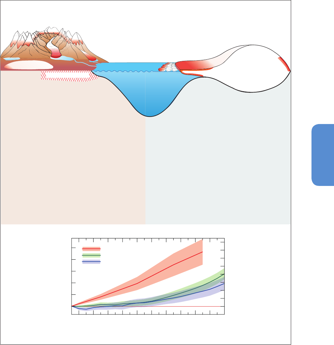
367

Observations: Cryosphere Chapter 4

4.8 Synthesis

Observations show that the cryosphere has been in transition during

the last few decades and that the strong and signiﬁcant changes

reported in AR4 have continued, and in many cases accelerated. The

number of in situ and satellite observations of cryospheric parame-

ters has increased considerably since AR4 and the use of the new data

in trend analyses, and also in process studies, has enabled increased

conﬁdence in the quantiﬁcation of most of the changes. A graphical

depiction and a text summary of observed changes in the various com-

ponents of the cryosphere are provided in Figure 4.25. They reveal a

general decline in all components of the cryosphere, but the magnitude

of the decline varies regionally and there are isolated cases where an

increase is observed.

Figure 4.25 | Schematic summary of the dominant observed variations in the cryosphere. The inset ﬁgure summarises the assessment of the sea level equivalent of ice loss from

the ice sheets of Greenland and Antarctica, together with the contribution from all glaciers except those in the periphery of the ice sheets (Section 4.3.3 and 4.4.2).

Changes in the Cryosphere

Ice Sheet

Sea Ice

Frozen Ground: increasing permafrost tempera-

tures by up to 2ºC and active layer thickness by up

to 90 cm since early 1980s. In the NH, southern limit

of permafrost moving north since mid 1970s, and

decreasing thickness of seasonal frozen ground by 32

cm since 1930s.

: between 1967 and 2012, satellite data showSnow cover

decreases through the year, with largest decreases (53%)

in June. Most stations report decreases in now especially

in spring.

: contracting winter ice duration withLake and river ice

delays in autumn freeze-up proceeding more slowly than

advances in spring break-up, with evidence of recent

acceleration in both across the NH.

are major contributors to sea level rise. Ice massGlaciers:

loss from glaciers has increased since the 1960s. Loss

rates from glaciers outside Greenland and Antarctica

were 0.76 mm yr SLE during the 1993 to 2009 period

-1

and 0.83 mm yr SLE over the 2005 to 2009 period.

-1

between 1979 and 2012, Arctic seaSea Ice:

ice extent declined at a rate of 3.8% per

decade with larger losses in summer and autumn.

Over the same period, the extent of thick multiyear

ice in the Arctic declined at a higher rate of 13.5% per

decade. Mean sea ice thickness decreased by 1.3 -

2.3 m between 1980 and 2008.

: continuing retreat andIce Shelves and ice tongues

collapse of ice shelves along theAntarctic Peninsula.

Progressive thinning of some other ice shelves/ice

tongues in Antarctica and Greenland.

: both Greenland and Antarctic ice sheetsIce Sheets

lost mass and contributed to sea level change over the

last 20 years. Rate of total loss and discharge from

a number of major outlet glaciers in Antarctica and

Greenland increased over this period.

Contribution of Glaciers and Ice Sheets to Sea Level Change

Ice Shelf

Glaciers

Snow Cover

Lake &

River Ice

Cumulative ice mass loss from glacier and ice sheets (in sea level equivalent) is

1.0 to 1.4 mm yr

-1

for 1993-2009 and 1.2 to 2.2 mm yr

-1

for 2005-2009.

Frozen Ground

1992 1994 1996 1998 2000 2002 2004 2006 2008 2010 2012

Year

Glaciers

Greenland

Antarctica

-2

SLE (mm)

1000

2000

3000

4000

5000

Cumulative ice mass loss (Gt)

368

Chapter 4 Observations: Cryosphere

Some of the observed changes since AR4 have been considerable and

unexpected. One of the most visible was the dramatic decline in the

September minimum sea ice cover in the Arctic in 2007, which was

followed by a record low value in 2012, supporting observations that

the thicker components of the Arctic sea ice cover are decreasing. The

trend in extent for Arctic sea ice is –3.8 ± 0.3% per decade (very likely)

while that for multi-year ice is –13.5 ± 2.5% per decade (very likely).

Observations also show marked decreases in Arctic ice thickness and

volume. The pattern of melt on the surface of the Greenland ice sheet

has also changed radically, with melt occurring in 2012 over almost the

entire surface of the ice sheet for the ﬁrst time during the satellite era.

The ice mass loss in Greenland has been observed to have increased

from 34 [–6 to 74] Gt yr

–1

for the period 1992–2001 to 215 [157 to

274] Gt yr

–1

for the period 2002–2011 while the estimates of mass

loss in Antarctica have increased from 30 [–37 to 97] Gt yr

–1

during the

1992–2001 period to 147 [72 to 221] Gt yr

–1

during the 2002–2011

period. Observed mass loss from glaciers has also increased, with the

global mass loss (excluding the glaciers peripheral to the ice sheets)

estimated to be 226 [91 to 361] Gt yr

–1

during the 1971–2009 period,

275 [140 to 410] Gt yr

–1

over the 1993–2009 period, and 301 [166 to

436] over the 2005–2009 period. A large majority of observing stations

report decreasing trends in snow depth, snow duration, or snow water

equivalent, and the largest decreases are typically observed at loca-

tions with temperatures close to freezing. Most lakes and rivers with

long-term records have exhibited declines in ice duration and average

seasonal ice cover. Permafrost has also been degrading and retreating

to the north while permafrost temperatures have increased in most

regions since the 1980s.

The observed positive trend of sea ice extent in the Antarctic that was

regarded as small and insigniﬁcant in AR4, has persisted, and increased

slightly to about 1.5 ± 0.2% per decade. The higher-than-average Ant-

arctic sea ice extent in recent years has been mainly due to increases

in the Ross Sea region, which more than offset the declines in the Bell-

ingshausen Sea and Amundsen Sea. Ice production in coastal polynyas

(regarded as ‘sea ice factories’) along the Ross Sea ice shelves have

been observed to be increasing. Recent work suggests strengthening

of the zonal (east-west) winds and accompanying ice drift accounts for

some of the increasing sea ice extent.

Satellite data have provided the ability to observe large-scale changes

in the cryosphere at relatively good temporal and spatial resolution

throughout the globe. Largely because of the availability of high reso-

lution satellite data, the ﬁrst near-complete global glacial inventory has

been generated, leading to a more precise determination of the past,

current and future contribution of glaciers to sea level rise. As more

data accumulate, and as more capable sensors are launched, the data

become more valuable for studies related to change assessment. The

advent of new satellites and airborne missions has provided powerful

tools that have enabled breakthroughs in the capability to measure

some parameters and enhance our ability to interpret results. However,

a longer record of measurements of the cryosphere will help increase

conﬁdence in the results, reduce uncertainties in the long-term trends,

and bring more critical insights into the physical processes controlling

the changes. There is thus a need for the continuation of the satellite

records, and a requirement for longer and more reliable historical data

from in situ measurements and proxies.

The sea level equivalent of mass loss from the Greenland and Antarctic

ice sheets over the period 1993–2010, has been about 5.9 mm (includ-

ing 1.7 mm from glaciers around Greenland) and 4.8 mm, respectively.

The reliability of observations of ice loss from the ice sheets has been

enhanced with the introduction of advanced satellite observation tech-

niques. The ice loss from glaciers between 1993 and 2009 measured

in terms of sea level equivalent (excluding those peripheral to the ice

sheets) is estimated to be 13 mm. The inset to Figure 4.25 shows the

cumulative sea level equivalent from glaciers and the ice sheets in

Greenland and Antarctica. These have been contributing dominantly to

sea level rise in recent decades. The contribution of the cryosphere to

sea level change is discussed more fully in Chapter 13.

The overall consistency in the negative changes observed in the vari-

ous components of the cryosphere (Figure 4.25), and the acceleration

of these changes in recent decades, provides a strong signal of climate

change. Regional differences in the magnitude and direction of the sig-

nals are apparent, but these are not unexpected considering the large

variability and complexity of atmospheric and oceanic circulations. It

is very likely, however, that the Arctic has changed substantially since

1979.

Acknowledgements

We acknowledge the kind contributions of C. Starr (NASA Visualization

Group), U. Blumthaler, S. Galos (University of Innsbruck) and P. Fretwell

(British Antarctic Survey), who assisted in drafting ﬁgures. M. Mahrer,

R. Graber (University of Zurich) and G. Hiess (BAS) undertook valuable

literature reviews, and N. E. Barrand (BAS) assisted with collation of

references.

369

Observations: Cryosphere Chapter 4

References

Abdalati, W., et al., 2004: Elevation changes of ice caps in the Canadian Arctic

Archipelago. J. Geophys. Res. Earth Surf., 109, 11 (F04007).

Abdalati, W., et al., 2010: The ICESat-2 Laser Altimetry Mission. Proc. IEEE, 98,

735–751.

Akerman, H. J., and M. Johansson, 2008: Thawing permafrost and thicker active

layers in sub-Arctic Sweden. Permafr. Process., 19, 279–292.

Allard, M., B. L. Wang, and J. A. Pilon, 1995: Recent cooling along the southern

shore of the Hudson Strait, Quebec, Canada, documented from permafrost

temperatuure-measurements. Arct. Alp. Res., 27, 157–166.

Alley, R. B., and S. Anandakrishnan, 1995: Variations in melt-layer frequency in

the GISP2 ice core: Implications for Holocene summer temperatures central

Greenland. Ann. Glaciol., 21, 64–70.

Alley, R. B., et al., 2008: A simple law for ice-shelf calving. Science, 322, 1344–1344.

Amundson, J. M., M. Fahnestock, M. Truffer, J. Brown, M. P. Luthi, and R. J. Motyka,

2010: Ice melange dynamics and implications for terminus stability, Jakobshavn

Isbrae Greenland. J. Geophys. Res. Earth Surf., 115, 12

Andresen, C. S., et al., 2012: Rapid response of Helheim Glacier in Greenland to

climate variability over the past century. Nature Geosci., 5, 37–41

Arendt, A. A., K. A. Echelmeyer, W. D. Harrison, C. S. Lingle, and V. B. Valentine, 2002:

Rapid wastage of Alaska glaciers and their contribution to rising sea level.

Science, 297, 382–386.

Arendt, A., et al., 2012: Randolph Glacier Inventory [v2.0]: A Dataset of Global

Glacier Outlines. Global Land Ice Measurements from Space, Boulder Colorado,

USA. Digital Media 32 pp. [Available online at: http://www.glims.org/RGI/RGI_

Tech_Report_V2.0.pdf]

Arthern, R. J., D. P. Winebrenner, and D. G. Vaughan, 2006: Antarctic snow

accumulation mapped using polarization of 4.3-cm wavelength microwave

emission. J. Geophys. Res. Atmos., 111, D06107.

Arthern, R. J., D. G. Vaughan, A. M. Rankin, R. Mulvaney, and E. R. Thomas, 2010:

In-situ measurements of Antarctic snow compaction, compared with predictions

of models. J. Geophys. Res., 115, F03011.

Azam, M. F., et al., 2012: From balance to imbalance: a shift in the dynamic behaviour

of Chhota Shigri glacier, western Himalaya, India. J. Glaciol., 58, 315–324.

Bahr, D. B., M. F. Meier, and S. D. Peckham, 1997: The physical basis of glacier volume-

area scaling. J. Geophys. Res. Sol. Ea., 102, 20355–20362.

Bahr, D. B., M. Dyurgerov, and M. F. Meier, 2009: Sea-level rise from glaciers and ice

caps: A lower bound. Geophys. Res. Lett., 36, 4 (L03501).

Bales, R. C., et al., 2009: Annual accumulation for Greenland updated using ice core

data developed during 2000–2006 and analysis of daily coastal meteorological

data. J. Geophys. Res. Atmos., 114, D06116.

Bamber, J. L., et al., 2013: A new bed elevation dataset for Greenland. Cryosphere,

7, 499–510.

Barrand, N., D. G. Vaughan, N. Steiner, M. Tedesco, P. Kuipers Munneke, M. R. van den

Broeke, and J. S. Hosking, 2013: Trends in Antarctic Peninsula surface melting

conditions from observations and regional climate modelling. J. Geophys. Res.,

118, 1–16.

Barrett, P. J., 2013: Resolving views on Antarctic Neogene glacial history—the Sirius

debate. Earth Environ. Sci. Trans. R. Soc. Edinburgh, 104, 29–51.

Barry, R., and T. Y. Gran, 2011: The Global Cryosphere: Past, Present and Future.

Cambridge University Press, Cambridge, UK, and New York, NY, USA, 498 pp.

Barry, R. G., R. E. Moritz, and J. C. Rogers, 1979: Fast ice regimes of the Beaufort and

Chukchi sea coasts, Alaska. Cold Reg. Sci. Technol., 1, 129–152.

Bartholomew, I. D., P. Nienow, A. Sole, D. Mair, T. Cowton, M. A. King, and S. Palmer,

2011: Seasonal variations in Greenland Ice Sheet motion: Inland extent and

behaviour at higher elevations. Earth Planet. Sci. Lett., 307, 271–278.

Baur, O., M. Kuhn, and W. E. Featherstone, 2009: GRACE-derived ice-mass variations

over Greenland by accounting for leakage effects. J. Geophys. Res. Sol. Ea., 114,

13 (B06407).

Belchansky, G. I., D. C. Douglas, and N. G. Platonov, 2004: Duration of the Arctic Sea

ice melt season: Regional and interannual variability, 1979–2001. J. Clim., 17,

67–80.

Beltaos, S., and T. Prowse, 2009: River-ice hydrology in a shrinking cryosphere.

Hydrol. Process., 23, 122–144.

Benn, D. I., C. R. Warren, and R. H. Mottram, 2007: Calving processes and the

dynamics of calving glaciers. Earth Sci. Rev., 82, 143–179.

Benson, B. J., et al., 2012: Extreme events, trends, and variability in Northern

Hemisphere lake-ice phenology (1855–2005). Clim. Change, 112, 299–323.

Berthier, E., E. Schiefer, G. K. C. Clarke, B. Menounos, and F. Remy, 2010: Contribution

of Alaskan glaciers to sea-level rise derived from satellite imagery. Nature

Geosci., 3, 92–95.

Bindschadler, R., et al., 2011: Getting around Antarctica: new high-resolution

mappings of the grounded and freely-ﬂoating boundaries of the Antarctic ice

sheet created for the International Polar Year. Cryosphere, 5, 569–588.

Bjørk, A. A., et al., 2012: An aerial view of 80 years of climate-related glacier

ﬂuctuations in southeast Greenland. Nature Geosci., 5, 427–432.

Björnsson, H., et al., 2013: Contribution of Icelandic ice caps to sea level rise: trends

and variability since the Little Ice Age. Geophys. Res. Lett., 40, 1546-1550

Blaszczyk, M., J. A. Jania, and J. O. Hagen, 2009: Tidewater glaciers of Svalbard:

Recent changes and estimates of calving ﬂuxes. Pol. Polar Res., 30, 85–142.

Bliss, A., R. Hock, and J. G. Cogley, 2013: A new inventory of mountain glaciers and

ice caps for the Antarctic periphery. Ann. Glaciol., 54, 191–199.

Bodin, X., F. Rojas, and A. Brenning, 2010: Status and evolution of the cryosphere in

the Andes of Santiago (Chile, 33.5 degrees S.). Geomorphology, 118, 453–464.

Bodin, X., et al., 2009: Two Decades of Responses (1986–2006) to Climate by the

Laurichard Rock Glacier, French Alps. Permafr. Periglac. Process., 20, 331–344.

Boening, C., M. Lebsock, F. Landerer, and G. Stephens, 2012: Snowfall-driven mass

change on the East Antarctic ice sheet. Geophys. Res. Lett., 39, L21501.

Boening, C. W., A. Dispert, M. Visbeck, S. R. Rintoul, and F. U. Schwarzkopf, 2008: The

response of the Antarctic Circumpolar Current to recent climate change. Nature

Geosci., 1, 864–869.

Bolch, T., B. Menounos, and R. Wheate, 2010: Landsat-based inventory of glaciers in

western Canada, 1985–2005. Remote Sens. Environ., 114, 127–137.

Bolch, T., L. Sandberg Sørensen, S. B. Simonsen, N. Moelg, H. Machguth, P. Rastner,

and F. Paul, 2013: Mass loss of Greenland’s glaciers and ice caps 2003–2008

revealed from ICESat data. Geophys. Res. Lett., 40, 875–881.

Bolch, T., et al., 2012: The state and fate of Himalayan glaciers. Science, 336, 310–

314.

Bown, F., A. Rivera, and C. Acuna, 2008: Recent glacier variations at the Aconcagua

basin, central Chilean Andes. Ann. Glaciol., 48, 43–48.

Box, J. E., L. Yang, D. H. Bromwich, and L. S. Bai, 2009: Greenland ice sheet surface air

temperature variability: 1840–2007. J. Clim., 22, 4029–4049.

Box, J. E., X. Fettweis, J. C. Stroeve, M. Tedesco, D. K. Hall, and K. Steffen, 2012:

Greenland ice sheet albedo feedback: Thermodynamics and atmospheric drivers.

Cryosphere, 6, 821–839.

Brewer, M. C., 1958: Some results of geothermal investigations of permafrost. Am.

Geophys. Union Trans. 39, 19–26.

Bromwich, D. H., J. P. Nicolas, and A. J. Monaghan, 2011: An assessment of

precipitation changes over Antarctica and the Southern Ocean since 1989 in

contemporary global reanalyses. J. Clim., 24, 4189–4209.

Bromwich, D. H., J. P. Nicolas, A. J. Monaghan, M. A. Lazzara, L. M. Keller, G. A.

Weidner, and A. B. Wilson, 2013: Central West Antarctica among the most rapidly

warming regions on Earth. Nature Geosci., 6, 139–145.

Brooks, R. N., T. D. Prowse, and I. J. O’Connell, 2012: Quantifying Northern Hemisphere

freshwater ice. Geophys. Res. Lett., 40, 1128–1131.

Brown, R., C. Derksen, and L. B. Wang, 2010: A multi-data set analysis of variability

and change in Arctic spring snow cover extent, 1967–2008. J. Geophys. Res.

Atmos., 115, D16111.

Brown, R. D., and P. Coté, 1992: Interannual variability of landfast ice thickness in the

Canadian High Arctic, 1950–89. Arctic, 45, 273–284.

Brown, R. D., and P. W. Mote, 2009: The response of Northern Hemisphere snow

cover to a changing climate. J. Clim., 22, 2124–2145.

Brown, R. D., and D. A. Robinson, 2011: Northern Hemisphere spring snow cover

variability and change over 1922–2010 including an assessment of uncertainty.

Cryosphere, 5, 219–229.

Brunt, K. M., E. A. Okal, and D. R. MacAyeal, 2011: Antarctic ice-shelf calving triggered

by the Honshu (Japan) earthquake and tsunami, March 2011. J. Glaciol., 57,

785–788.

Buchardt, S. L., H. B. Clausen, B. M. Vinther, and D. Dahl-Jensen, 2012: Investigating

the past and recent delta18O-accumulation relationship seen in Greenland ice

cores. Clim. Past, 8, 2053–2059.

370

Chapter 4 Observations: Cryosphere

Bulygina, O. N., V. N. Razuvaev, and N. N. Korshunova, 2009: Changes in snow cover

over Northern Eurasia in the last few decades. Environ. Res. Lett., 4, 045026.

Bulygina, O. N., P. Y. Groisman, V. N. Razuvaev, and N. N. Korshunova, 2011: Changes

in snow cover characteristics over Northern Eurasia since 1966. Environ. Res.

Lett., 6, 045204.

Burn, C. R., and S. V. Kokelj, 2009: The environment and permafrost of the Mackenzie

Delta Area. Permafr. Periglac. Process., 20, 83–105.

Burn, C. R., and Y. Zhang, 2009: Permafrost and climate change at Herschel Island

(Qikiqtaruq), Yukon Territory, Canada. J. Geophys. Res., 114, F02001.

Callaghan, T. V., F. Bergholm, T. R. Christensen, C. Jonasson, U. Kokfelt, and M.

Johansson, 2010: A new climate era in the sub-Arctic: Accelerating climate

changes and multiple impacts. Geophys. Res. Lett., 37, L14705.

Callaghan, T. V., M. Johansson, O. Anisimov, H. H. Christiansen, A. Instanes, V.

Romanovsky, and S. Smith, 2011: Changing permafrost and its impacts. In:

Snow, Water, Ice and Permafrost in the Arctic (SWIPA). Arctic Monitoring and

Assessment Program (AMAP).

Carrivick, J. L., B. J. Davies, N. F. Glasser, D. Nyvlt, and M. J. Hambrey, 2012: Late-

Holocene changes in character and behaviour of land-terminating glaciers on

James Ross Island, Antarctica. J. Glaciol., 58, 1176–1190.

Carturan, L., and R. Seppi, 2007: Recent mass balance results and morphological

evolution of Careser glacier (Central Alps). Geograf. Fis. Dinam. Quat., 30, 33–42.

Cavalieri, D. J., and C. L. Parkinson, 2012: Arctic sea ice variability and trends, 1979–

2010. Cryosphere, 6, 957–979.

Cavalieri, D. J., P. Gloersen, and W. J. Campbell, 1984: Determination of sea ice

parameters with the Nimbus-7 SMMR. J. Geophys. Res. Atmos., 89, 5355–5369.

Cazenave, A., et al., 2009: Sea level budget over 2003–2008: A reevaluation from

GRACE space gravimetry, satellite altimetry and Argo. Global Planet. Change,

65, 83–88.

Chapman, W. L., and J. E. Walsh, 2007: A synthesis of Antarctic temperatures. J. Clim.,

20, 4096–4117.

Charrassin, J. B., et al., 2008: Southern Ocean frontal structure and sea-ice formation

rates revealed by elephant seals. Proc. Natl. Acad. Sci. U.S.A., 105, 11634–11639.

Chen, J. L., C. R. Wilson, and B. D. Tapley, 2006: Satellite gravity measurements

conﬁrm accelerated melting of Greenland ice sheet. Science, 313, 1958–1960.

Chen, J. L., C. R. Wilson, and B. D. Tapley, 2011: Interannual variability of Greenland

ice losses from satellite gravimetry. J. Geophys. Res. Sol. Ea., 116, 11( B07406).

Chen, J. L., C. R. Wilson, D. Blankenship, and B. D. Tapley, 2009: Accelerated Antarctic

ice loss from satellite gravity measurements. Nature Geosci., 2, 859–862.

Chen, J. L., C. R. Wilson, B. D. Tapley, D. D. Blankenship, and E. R. Ivins, 2007: Patagonia

iceﬁeld melting observed by gravity recovery and climate experiment (GRACE).

Geophys. Res. Lett., 34, 6 (L22501).

Cheng, G. D., and T. H. Wu, 2007: Responses of permafrost to climate change and

their environmental signiﬁcance, Qinghai-Tibet Plateau. J. Geophys. Res., 112,

F02S03.

Chinn, T., S. Winkler, M. J. Salinger, and N. Haakensen, 2005: Srecent glacier

advances in Norway and New Zealand: A comparison of their glaciological and

meteorological causes. Geograf. Annal. A, 87A, 141–157.

Choi, G., D. A. Robinson, and S. Kang, 2010: Changing Northern Hemisphere snow

seasons. J. Clim., 23, 5305–5310.

Christiansen, H. H., M. Guglielmin, J. Noetzli, V. Romanovsky, N. Shiklomanov, S.

Smith, and L. Zhao, 2012: Cryopsphere, Permafrost thermal state. Special Suppl.

to Bull. Am. Meteorol. Soc., 93( July) [J. Blunden and D. S. Arndt (eds.)], S19–S21.

Christiansen, H. H., et al., 2010: The thermal state of permafrost in the Nordic area

during the International Polar Year 2007–2009. Permafr. Periglac. Process., 21,

156–181.

Christoffersen, P., et al., 2011: Warming of waters in an East Greenland fjord prior

to glacier retreat: Mechanisms and connection to large-scale atmospheric

conditions. Cryosphere, 5, 701–714.

Christy, J. R., 2012: Searching for information in 133 years of California snowfall

observations. J. Hydrometeorol., 13, 895–912.

Citterio, M., F. Paul, A. P. Ahlstrom, H. F. Jepsen, and A. Weidick, 2009: Remote sensing

of glacier change in West Greenland: accounting for the occurrence of surge-

type glaciers. Ann. Glaciol., 50, 70–80.

Citterio, M., G. Diolaiuti, C. Smiraglia, C. D’Agata, T. Carnielli, G. Stella, and G. B.

Siletto, 2007: The ﬂuctuations of Italian glaciers during the last century: A

contribution to knowledge about Alpine glacier changes. Geograf. Annal. A,

89A, 167–184.

Cogley, J. G., 2009a: A more complete version of the World Glacier Inventory. Ann.

Glaciol., 50, 32–38.

Cogley, J. G., 2009b: Geodetic and direct mass-balance measurements: comparison

and joint analysis. Ann. Glaciol., 50, 96–100.

Cogley, J. G., 2012: Area of the ocean. Mar. Geodesy, 35, 379–388.

Cogley, J. G., et al., 2011: Glossary of Glacier Mass Balance and Related Terms.

IHP-VII Technical Documents in Hydrology No. 86, International Association of

Cryospheric Sciences, Contribution No. 2, UNESCO-IHP. 114 pp.

Comiso, J. C., 2002: A rapidly declining perennial sea ice cover in the Arctic. Geophys.

Res. Lett., 29, 1956.

Comiso, J. C., 2010: Polar Oceans from Space. Springer Science+Business Media,

New York, NY, USA and Heidelberg, Germany.

Comiso, J. C., 2012: Large decadal decline in the Arctic multiyear ice cover. J. Clim.,

25, 1176–1193.

Comiso, J. C., and F. Nishio, 2008: Trends in the sea ice cover using enhanced and

compatible AMSR-E, SSM/I, and SMMR data. J. Geophys. Res. Oceans, 113,

C02S07.

Comiso, J. C., C. L. Parkinson, R. Gersten, and L. Stock, 2008: Accelerated decline in

the Arctic Sea ice cover. Geophys. Res. Lett., 35, L01703.

Comiso, J. C., R. Kwok, S. Martin, and A. L. Gordon, 2011: Variability and trends in

sea ice extent and ice production in the Ross Sea. J. Geophys. Res. Oceans, 116,

C04021.

Cook, A. J., and D. G. Vaughan, 2010: Overview of areal changes of the ice shelves on

the Antarctic Peninsula over the past 50 years. Cryosphere, 4, 77–98.

Costa, D. P., J. M. Klinck, E. E. Hofmann, M. S. Dinniman, and J. M. Burns, 2008:

Upper ocean variability in west Antarctic Peninsula continental shelf waters as

measured using instrumented seals. Deep-Sea Res. Pt. Ii, 55, 323–337.

Coudrain, A., B. Francou, and Z. W. Kundzewicz, 2005: Glacier shrinkage in the Andes

and consequences for water resources. Hydrol. Sci. J. –J. Sci. Hydrol., 50, 925–932.

Cullen, N. J., P. Sirguey, T. Moelg, G. Kaser, M. Winkler, and S. J. Fitzsimons, 2013:

A century of ice retreat on Kilimanjaro: The mapping reloaded. Cryosphere, 7,

419–431.

Daniault, N., H. Mercier, and P. Lherminier, 2011: The 1992–2009 transport variability

of the East Greenland-Irminger Current at 60 degrees N. Geophys. Res. Lett.,

38, 4 (L07601).

Das, S. B., I. Joughin, M. D. Behn, I. M. Howat, M. A. King, D. Lizarralde, and M.

P. Bhatia, 2008: Fracture propagation to the base of the Greenland Ice Sheet

during supraglacial lake drainage. Science, 320, 778–781.

Davies, B. J., and N. F. Glasser, 2012: Accelerating shrinkage of Patagonian glaciers

from the “Little Ice Age” (c. AD 1870) to 2011. J. Glaciol., 58, 1063–1084.

De Angelis, H., and P. Skvarca, 2003: Glacier surge after ice shelf collapse. Science,

299, 1560–1562.

Delaloye, R., et al., cited 2011: Recent interannual variations of rock glacier creep in

the European Alps. [Available online at http://www.zora.uzh.ch/7031/.]

DeLiberty, T. L., C. A. Geiger, S. F. Ackley, A. P. Worby, and M. L. Van Woert, 2011:

Estimating the annual cycle of sea-ice thickness and volume in the Ross Sea.

Deep-Sea Res. Pt. Ii, 58, 1250–1260.

Derksen, C., and R. Brown, 2012: Spring snow cover extent reductions in the

2008–2012 period exceeding climate model projections. Geophys. Res. Lett., 39,

L19504.

Derksen, C., et al., 2012: Variability and change in the Canadian cryosphere. Clim.

Change, 115, 59–88.

Déry, S. J., and R. D. Brown, 2007: Recent Northern Hemisphere snow cover extent

trends and implications for the snow-albedo feedback. Geophys. Res. Lett., 34,

6 (L22504).

Ding, Q. H., E. J. Steig, D. S. Battisti, and M. Kuttel, 2011: Winter warming in West

Antarctica caused by central tropical Paciﬁc warming. Nature Geosci., 4, 398–

403.

Dinniman, M. S., J. M. Klinck, and E. E. Hofmann, 2012: Sensitivity of circumpolar

deep water transport and ice shelf basal melt along the West Antarctic Peninsula

to changes in the winds. J. Clim., 25, 4799–4816.

Diolaiuti, G., D. Bocchiola, C. D’Agata, and C. Smiraglia, 2012: Evidence of climate

change impact upon glaciers’ recession within the Italian Alps—The case of

Lombardy glaciers. Theor. Appl. Climatol., 109, 429–445.

Dmitrenko, I. A., et al., 2011: Recent changes in shelf hydrography in the Siberian

Arctic: Potential for subsea permafrost instability. J. Geophys. Res. Oceans, 116,

10 (C10027).

Doake, C. S. M., and D. G. Vaughan, 1991: Rapid disintegration of the wordie ice shelf

in response to atmospheric warming. Nature, 350, 328–330.

371

Observations: Cryosphere Chapter 4

Doake, C. S. M., H. F. J. Corr, H. Rott, P. Skvarca, and N. W. Young, 1998: Breakup and

conditions for stability of the northern Larsen Ice Shelf, Antarctica. Nature, 391,

778–780.

Doherty, S. J., S. G. Warren, T. C. Grenfell, A. D. Clarke, and R. E. Brandt, 2010: Light-

absorbing impurities in Arctic snow. Atmos. Chem. Phys., 10, 11647–11680.

Drobot, S. D., and M. R. Anderson, 2001: An improved method for determining

snowmelt onset dates over Arctic sea ice using scanning multichannel

microwave radiometer and Special Sensor Microwave/Imager data. J. Geophys.

Res. Atmos., 106, 24033–24049.

Drozdov, D. S., N. G. Ukraintseva, A. M. Tsarev, and S. N. Chekrygina, 2010: Changes

in the temperature ﬁeld and in the state of the geosystems within the territory

of the Urengoy ﬁeld during the last 35 years (1974–2008). Earth Cryosphere,

14, 22–31.

Druckenmiller, M. L., H. Eicken, M. A. Johnson, D. J. Pringle, and C. C. Williams, 2009:

Toward an integrated coastal sea-ice observatory: System components and a

case study at Barrow, Alaska. Cold Reg. Sci. Technol., 56, 61–72.

Drucker, R., S. Martin, and R. Kwok, 2011: Sea ice production and export from coastal

polynyas in the Weddell and Ross Seas. Geophys. Res. Lett., 38, 4 (L17502).

Ducklow, H., et al., 2011: The marine system of the Western Antarctic Peninsula In:

Antarctica: An Extreme Environment in a Changing World [A. D. Rogers (ed.)].

New York, NY, USA, John Wiley & Sons. 121-159.

E, D.-C., Y.-D. Yang, and D.-B. Chao, 2009: The sea level change from the Antarctic ice

sheet based on GRACE. Chin. J. Geophys.–Chin. Ed., 52, 2222–2228.

Ettema, J., M. R. van den Broeke, E. van Meijgaard, W. J. van de Berg, J. L. Bamber,

J. E. Box, and R. C. Bales, 2009: Higher surface mass balance of the Greenland

ice sheet revealed by high-resolution climate modeling. Geophys. Res. Lett., 36,

L12501.

Ewert, H., A. Groh, and R. Dietrich, 2012: Volume and mass changes of the Greenland

ice sheet inferred from ICESat and GRACE. J. Geodyn., 59, 111–123.

Fedorov, A. N., and P. Y. Konstantinov, 2008: Recent changes in ground temperature

and the effect on permafrost landscapes in Central Yakutia. In: Proceeding of

the 9th International Conference on Permafrost, 29 June–3 July 2008, Institute

of Northern Engineering, University of Alaska, Fairbanks [D. L. Kane, and K. M.

Hinkel (eds.)], pp. 433–438.

Fernandes, R., H. X. Zhao, X. J. Wang, J. Key, X. Qu, and A. Hall, 2009: Controls on

Northern Hemisphere snow albedo feedback quantiﬁed using satellite Earth

observations. Geophys. Res. Lett., 36, L21702.

Fettweis, X., M. Tedesco, M. R. van den Broeke, and J. Ettema, 2011: Melting trends

over the Greenland ice sheet (1958–2009) from spaceborne microwave data

and regional climate models. Cryosphere, 5, 359–375.

Flament, T., and F. Remy, 2012: Dynamic thinning of Antarctic glaciers from along-

track repeat radar altimetry. J. Glaciol., 58, 830–840.

Flanner, M. G., C. S. Zender, J. T. Randerson, and P. J. Rasch, 2007: Present-day climate

forcing and response from black carbon in snow. J. Geophys. Res., 112, D11202.

Flanner, M. G., K. M. Shell, M. Barlage, D. K. Perovich, and M. A. Tschudi, 2011:

Radiative forcing and albedo feedback from the Northern Hemisphere

cryosphere between 1979 and 2008. Nature Geosci., 4, 151–155.

Fleming, K., and K. Lambeck, 2004: Constraints on the Greenland Ice Sheet since the

Last Glacial Maximum from sea-level observations and glacial-rebound models.

Quat. Sci. Rev., 23, 1053–1077.

Foster, J. L., D. K. Hall, R. E. J. Kelly, and L. Chiu, 2009: Seasonal snow extent and

snow mass in South America using SMMR and SSM/I passive microwave data

(1979–2006). Remote Sens. Environ., 113, 291–305.

Fraser, A. D., R. A. Massom, K. J. Michael, B. K. Galton-Fenzi, and J. L. Lieser, 2012:

East Antarctic landfast sea ice distribution and variability, 2000–2008. J. Clim.,

25, 1137–1156.

Frauenfeld, O. W., and T. J. Zhang, 2011: An observational 71-year history of

seasonally frozen ground changes in the Eurasian high latitudes. Environ. Res.

Lett., 6, 044024.

Frauenfeld, O. W., T. J. Zhang, R. G. Barry, and D. Gilichinsky, 2004: Interdecadal

changes in seasonal freeze and thaw depths in Russia. J. Geophys. Res., 109,

D05101.

Fretwell, P. T., et al., 2013: Bedmap2: improved ice bed, surface and thickness

datasets for Antarctica. Cryosphere, 7, 375–393.

Frezzotti, M., C. Scarchilli, S. Becagli, M. Proposito, and S. Urbini, 2012: A synthesis of

the Antarctic Surface Mass Balance during the last eight centuries. Cryosphere,

7, 303–319.

Fricker, H. A., and L. Padman, 2012: Thirty years of elevation change on Antarctic

Peninsula ice shelves from multimission satellite radar altimetry. J. Geophys. Res.

Oceans, 117, C02026.

Fyodorov-Davydov, D. G., A. L. Kholodov, V. E. Ostroumov, G. N. Kraev, V. A. Sorokovikov,

S. P. Davudov, and A. A. Merekalova, 2008: Seasonal thaw of soils in the North

Yakutian ecosystems. In: Proceedings of the 9th International Conference on

Permafrost, 29 June– 3 July 2008, Institute of Northern Engineering, University

of Alaska, Fairbanks [D. L. Kane, and K. M. Hinkel (eds.)], pp. 481–486.

Galton-Fenzi, B. K., J. R. Hunter, R. Coleman, and N. Young, 2012: A decade of change

in the hydraulic connection between an Antarctic epishelf lake and the ocean. J.

Glaciol., 58, 223–228.

Gardelle, J., E. Berthier, and Y. Arnaud, 2012: Slight mass gain of Karakoram glaciers

in the early twenty-ﬁrst century. Nature Geosci., 5, 322–325.

Gardner, A., G. Moholdt, A. Arendt, and B. Wouters, 2012: Accelerated contributions

of Canada’s Bafﬁn and Bylot Island glaciers to sea level rise over the past half

century. Cryosphere, 6, 1103–1125.

Gardner, A. S., et al., 2011: Sharply increased mass loss from glaciers and ice caps in

the Canadian Arctic Archipelago. Nature, 473, 357–360.

Gardner, A. S., et al., 2013: A reconciled estimate of glacier contributions to sea level

rise: 2003 to 2009. Science, 340, 852–857.

Gerland, S., A. H. H. Renner, F. Godtliebsen, D. Divine, and T. B. Loyning, 2008: Decrease

of sea ice thickness at Hopen, Barents Sea, during 1966–2007. Geophys. Res.

Lett., 35, L06501.

Gilbert, A., P. Wagnon, C. Vincent, P. Ginot, and M. Funk, 2010: Atmospheric warming

at a high-elevation tropical site revealed by englacial temperatures at Illimani,

Bolivia (6340 m above sea level, 16 degrees S, 67 degrees W). J. Geophys. Res.,

115, D10109.

Giles, A. B., R. A. Massom, and V. I. Lytle, 2008a: Fast-ice distribution in East

Antarctica during 1997 and 1999 determined using RADARSAT data. J. Geophys.

Res. Oceans, 113, 15 (C02S14).

Giles, K. A., S. W. Laxon, and A. L. Ridout, 2008b: Circumpolar thinning of Arctic

sea ice following the 2007 record ice extent minimum. Geophys. Res. Lett., 35,

L22502.

Gille, S. T., 2002: Warming of the Southern Ocean since the 1950s. Science, 295,

1275–1277.

Gille, S. T., 2008: Decadal-scale temperature trends in the Southern Hemisphere

Ocean. J. Clim., 21, 4749–4765.

Glazovsky, A., and Y. Macheret, 2006: Eurasian Arctic. In: Glaciation in North and

Central Eurasia in Present Time. [V. M. Kotlyakov (ed.)]. Nauka, Saint Petersburg,

Russian Federation, pp. 438–445.

Gordon, A. L., M. Visbeck, and J. C. Comiso, 2007: A possible link between the

Weddell Polynya and the Southern Annular Mode. J. Clim., 20, 2558–2571.

Grebmeier, J. M., S. E. Moore, J. E. Overland, K. E. Frey, and R. Gradinger, 2010:

Biological response to recent Paciﬁc Arctic sea ice retreats. EOS Trans. Am.

Geophys. Union, 91, 161–163.

Green, K., 2011: Interannual and seasonal changes in the ice cover of glacial lakes in

the Snowy Mountains of Australia. J. Mount. Sci., 8, 655–663.

Gregory, J. M., and J. Oerlemans, 1998: Simulated future sea-level rise due to glacier

melt based on regionally and seasonally resolved temperature changes. Nature,

391, 474–476.

Griggs, J., and J. L. Bamber, 2011: Antarctic ice-shelf thickness from satellite radar

altimetry. J. Glaciol., 57, 485–498.

Grinsted, A., 2013: An estimate of global glacier volume. Cryosphere, 7, 141–151.

Gruber, S., 2012: Derivation and analysis of a high-resolution estimate of

globalpermafrost zonation. Cryosphere, 6, 221–233.

Gruber, S., and W. Haeberli, 2007: Permafrost in steep bedrock slopes and its

temperature-related destabilization following climate change. J. Geophys. Res.,

112, 10 (F02S18).

Guglielmin, M., and N. Cannone, 2012: A permafrost warming in a cooling

Antarctica? Clim. Change, 111, 177–195.

Guglielmin, M., M. R. Balks, L. S. Adlam, and F. Baio, 2011: Permafrost thermal regime

from two 30-m deep boreholes in Southern Victoria Land, Antarctica. Permafr.

Periglac. Process., 22, 129–139.

Gunter, B., et al., 2009: A comparison of coincident GRACE and ICESat data over

Antarctica. J. Geodesy, 83, 1051–1060.

Gusmeroli, A., P. Jansson, R. Pettersson, and T. Murray, 2012: Twenty years of cold

surface layer thinning at Storglaciären, sub-Arctic Sweden, 1989–2009. J.

Glaciol., 58, 3–10.

372

Chapter 4 Observations: Cryosphere

Haas, C., S. Hendricks, H. Eicken, and A. Herber, 2010: Synoptic airborne thickness

surveys reveal state of Arctic sea ice cover. Geophys. Res. Lett., 37, L09501.

Haas, C., H. Le Goff, S. Audrain, D. Perovich, and J. Haapala, 2011: Comparison of

seasonal sea-ice thickness change in the Transpolar Drift observed by local ice

mass-balance observations and ﬂoe-scale EM surveys. Ann. Glaciol., 52, 97–102.

Haas, C., A. Pfafﬂing, S. Hendricks, L. Rabenstein, J. L. Etienne, and I. Rigor, 2008:

Reduced ice thickness in Arctic Transpolar Drift favors rapid ice retreat. Geophys.

Res. Lett., 35, L17501.

Haeberli, W., M. Hoelzle, F. Paul, and M. Zemp, 2007: Integrated monitoring of

mountain glaciers as key indicators of global climate change: the European Alps.

Ann. Glaciol., 46, 150–160.

Haeberli, W., et al., 2006: Permafrost creep and rock glacier dynamics. Permafr.

Periglac. Process., 17, 189–214.

Haeberli, W., et al., 2010: Mountain permafrost: development and challenges of a

young research ﬁeld. J. Glaciol., 56, 1043–1058.

Hagg, W., C. Mayer, A. Lambrecht, D. Kriegel, and E. Azizov, 2012: Glacier changes

in the Big Naryn basin, Central Tian Shan. Global Planet. Change, doi:10.1016/j.

gloplacha.2012.07.010.

Hall, D. K., J. C. Comiso, N. E. DiGirolamo, C. A. Shuman, J. E. Box, and L. S. Koenig,

2013: Variability in the surface temperature and melt extent of the Greenland Ice

Sheet from MODIS. Geophys. Res. Lett., 10, 2114-2120.

Halsey, L. A., D. H. Vitt, and S. C. Zoltai, 1995: Disequilibrium response of permafrost

in boreal continental western Canada to climate-change. Clim. Change, 30,

57–73.

Hanna, E., et al., 2011: Greenland Ice Sheet surface mass balance 1870 to 2010

based on Twentieth Century Reanalysis, and links with global climate forcing. J.

Geophys. Res., 116, D24121.

Harig, C., and F. J. Simons, 2012: Mapping Greenland’s mass loss in space and time.

Proc. Natl. Acad. Sci. U.S.A., 109, 19934–19937.

Heid, T., and A. Kääb, 2012: Repeat optical satellite images reveal widespread and

long term decrease in land-terminating glacier speeds. Cryosphere , 6, 467–478

Hirabayashi, Y., S. Kanae, K. Masuda, K. Motoya, and P. Doell, 2008: A 59-year (1948–

2006) global near-surface meteorological data set for land surface models. Part

I: Development of daily forcing and assessment of precipitation intensity. Hydrol.

Res. Lett., 2, 36–40.

Hirabayashi, Y., Y. Zhang, S. Watanabe, S. Koirala, and S. Kanae, 2013: Projection of

glacier mass changes under a high-emission climate scenario using the global

glacier model HYOGA2. Hydrol. Res. Lett., 7, 6–11.

Hock, R., M. de Woul, V. Radic, and M. Dyurgerov, 2009: Mountain glaciers and ice

caps around Antarctica make a large sea-level rise contribution. Geophys. Res.

Lett., 36, L07501.

Hodgkins, A. G., I. C. James, and T. G. Huntington, 2002: Historical changes in lake

ice-out dates as indicators of climate change in New England, 1850–2000. Int.

J. Clim., 22, 1819–1827.

Hoelzle, M., G. Darms, M. P. Lüthi, and S. Suter, 2011: Evidence of accelerated

englacial warming in the Monte Rosa area, Switzerland/Italy. Cryosphere, 5,

231–243.

Hoffman, M. J., G. A. Catania, T. A. Neumann, L. C. Andrews, and J. A. Rumrill, 2011:

Links between acceleration, melting, and supraglacial lake drainage of the

western Greenland Ice Sheet. J. Geophys. Res. Earth Surf., 116, F04035.

Holland, D. M., and A. Jenkins, 1999: Modeling thermodynamic ice-ocean interactions

at the base of an ice shelf. J. Phys. Oceanogr., 29, 1787–1800.

Holland, D. M., R. H. Thomas, B. De Young, M. H. Ribergaard, and B. Lyberth, 2008:

Acceleration of Jakobshavn Isbrae triggered by warm subsurface ocean waters.

Nature Geosci., 1, 659–664.

Holland, P. R., and R. Kwok, 2012: Wind-driven trends in Antarctic sea ice motion.

Nature Geosci., 5, 872–875.

Holland, P. R., A. Jenkins, and D. M. Holland, 2010: Ice and ocean processes in the

Bellingshausen Sea, Antarctica. J. Geophys. Res. Oceans, 115, C05020.

Holland, P. R., H. F. J. Corr, H. D. Pritchard, D. G. Vaughan, R. J. Arthern, A. Jenkins,

and M. Tedesco, 2011: The air content of Larsen Ice Shelf. Geophys. Res. Lett.,

38, L10503.

Holzhauser, H., M. Magny, and H. J. Zumbuhl, 2005: Glacier and lake-level variations

in west-central Europe over the last 3500 years. Holocene, 15, 789–801.

Horwath, M., and R. Dietrich, 2009: Signal and error in mass change inferences from

GRACE: The case of Antarctica. Geophys. J. Int., 177, 849–864.

Howat, I. M., I. Joughin, and T. A. Scambos, 2007: Rapid changes in ice discharge

from Greenland outlet glaciers. Science, 315, 1559–1561.

Howat, I. M., I. Joughin, M. Fahnestock, B. E. Smith, and T. A. Scambos, 2008:

Synchronous retreat and acceleration of southeast Greenland outlet glaciers

2000–06: Ice dynamics and coupling to climate. J. Glaciol., 54, 646–660.

Howat, I. M., Y. Ahn, I. Joughin, M. R. van den Broeke, J. T. M. Lenaerts, and B. Smith,

2011: Mass balance of Greenland’s three largest outlet glaciers, 2000–2010.

Geophys. Res. Lett., 38, 5 (L12501).

Hudson, S. R., 2011: Estimating the global radiative impact of the sea ice-albedo

feedback in the Arctic. J. Geophys. Res. Atmos., 116, D16102.

Hughes, T. J., 1973: Is the West Antarctic ice sheet disintegrating? J. Geophys. Res.,

78, 7884–7910.

Hulbe, C. L., T. A. Scambos, T. Youngberg, and A. K. Lamb, 2008: Patterns of glacier

response to disintegration of the Larsen B ice shelf, Antarctic Peninsula. Global

Planet. Change, 63, 1–8.

Humbert, A., et al., 2010: Deformation and failure of the ice bridge on the Wilkins Ice

Shelf, Antarctica. Ann. Glaciol., 51, 49–55.

Hurrell, J. W., 1995: Decadal trends in the North-Atlantic oscillation—regional

temperatures and precipitation. Science, 269, 676–679.

Huss, M., 2012: Extrapolating glacier mass balance to the mountain-range scale: The

European Alps 1900–2100. Cryosphere, 6, 713–727.

Huss, M., and D. Farinotti, 2012: Distributed ice thickness and volume of 180,000

glaciers around the globe. J. Geophys. Res., 117, F04010.

Isaksen, K., et al., 2011: Degrading mountain permafrost in southern Norway: Spatial

and temporal variability of mean ground temperatures, 1999–2009. Permafr.

Periglac. Process., 22, 361–377.

Ishikawa, M., N. Sharkhuu, Y. Jambaljav, G. Davaa, K. Yoshikawa, and T. Ohata,

2012: Thermal state of Mongolian permafrost. In: Proceedings of the 10th

International Conference on Permafrost, June, 2012, Salekhard, Yamel-nenets

Autonomous District, Russian Federation, v1.[K. M. Hinkel (ed)]. The Northern

Publisher, Salekhard, Russia, pp. 173–178.

Ishizaka, M., 2004: Climatic response of snow depth to recent warmer winter

seasons in heavy-snowfall areas in Japan. Ann. Glaciol., 38, 299–304.

Ivins, E. R., and T. S. James, 2005: Antarctic glacial isostatic adjustment: A new

assessment. Antarct. Sci., 17, 541–553.

Ivins, E. R., M. M. Watkins, D. N. Yuan, R. Dietrich, G. Casassa, and A. Rulke, 2011:

On-land ice loss and glacial isostatic adjustment at the Drake Passage: 2003–

2009. J. Geophys. Res. Sol. Ea., 116, 24 (B02403).

Jacob, T., J. Wahr, W. T. Pfeffer, and S. Swenson, 2012: Recent contributions of glaciers

and ice caps to sea level rise. Nature, 482, 514–518.

Jacobs, S. S., A. Jenkins, C. F. Giulivi, and P. Dutrieux, 2011: Stronger ocean circulation

and increased melting under Pine Island Glacier ice shelf. Nature Geosci., 4,

519–523.

Jacobs, S. S., H. H. Helmer, C. S. M. Doake, A. Jenkins, and R. M. Frolich, 1992: Melting

of the ice shelves and the mass balance of Antarctica. J. Glaciol., 38, 375–387.

Jenkins, A., 2011: Convection-driven melting near the grounding lines of ice shelves

and tidewater glaciers. J. Clim., 41, 2279–2294.

Jenkins, A., and C. S. M. Doake, 1991: Ice-Ocean interaction on Ronne ice shelf,

Antarctica J. Geophys. Res. Oceans, 96, 791–813.

Jenkins, A., and S. Jacobs, 2008: Circulation and melting beneath George VI Ice Shelf,

Antarctica. J. Geophys. Res. Oceans, 113, C04013.

Jenkins, A., P. Dutrieux, S. S. Jacobs, S. D. McPhail, J. R. Perrett, A. T. Webb, and D.

White, 2010: Observations beneath Pine Island Glacier in West Antarctica and

implications for its retreat. Nature Geosci., 3, 468–472.

Jensen, O. P., B. J. Benson, J. J. Magnuson, V. M. Card, M. N. Futter, P. A. Soranno,

and K. M. Stewart, 2007: Spatial analysis of ice phenology trends across the

Laurentian Great Lakes Region during a recent warming period. Limnol.

Oceanogr., 52, 2013–2026.

Jia, L. L., H. S. Wang, and L. W. Xiang, 2011: Effect of glacio-static adjustment on the

estimate of ice mass balance over Antarctic and uncertainties. Chin. J. Geophys.,

54, 1466–1477.

Johannessen, O. M., E. V. Shalina, and M. W. Miles, 1999: Satellite evidence for an

Arctic sea ice cover in transformation. Science, 286, 1937–1939.

Johnson, J. S., M. J. Bentley, and K. Gohl, 2008: First exposure ages from the

Amundsen Sea embayment, West Antarctica: The late quaternary context for

recent thinning of Pine Island, Smith, and Pope Glaciers. Geology, 36, 223–226.

Jones, B. M., C. D. Arp, M. T. Jorgenson, K. M. Hinkel, J. A. Schmutz, and P. L. Flint,

2009: Increase in the rate and uniformity of coastline erosion in Arctic Alaska.

Geophys. Res. Lett., 36, 5 (L03503).

373

Observations: Cryosphere Chapter 4

Jones, P. D., D. H. Lister, T. J. Osborn, C. Harpham, M. Salmon, and C. P. Morice,

2012: Hemispheric and large-scale land-surface air temperature variations: An

extensive revision and an update to 2010. J. Geophys. Res. Atmos., 117, D05127.

Jorgenson, M. T., Y. L. Shur, and E. R. Pullman, 2006: Abrupt increase in permafrost

degradation in Arctic Alaska. Geophys. Res. Lett., 33, 4 (L02503).

Joughin, I., and R. B. Alley, 2011: Stability of the West Antarctic ice sheet in a

warming world. Nature Geosci., 4, 506–513.

Joughin, I., W. Abdalati, and M. Fahnestock, 2004: Large ﬂuctuations in speed on

Greenland’s Jakobshavn Isbrae glacier. Nature, 432, 608–610.

Joughin, I., B. E. Smith, and D. M. Holland, 2010a: Sensitivity of 21st century sea

level to ocean-induced thinning of Pine Island Glacier, Antarctica. Geophys. Res.

Lett., 37, L20502.

Joughin, I., R. B. Alley, and D. M. Holland, 2012: Ice-sheet response to oceanic

forcing. Science, 338, 1172–1176.

Joughin, I., M. Fahnestock, R. Kwok, P. Gogineni, and C. Allen, 1999: Ice ﬂow of

Humboldt, Petermann and Ryder Gletscher, northern Greenland. J. Glaciol., 45,

231–241.

Joughin, I., B. E. Smith, I. M. Howat, T. Scambos, and T. Moon, 2010b: Greenland ﬂow

variability from ice-sheet-wide velocity mapping. J. Glaciol., 56, 415–430.

Joughin, I., S. B. Das, M. A. King, B. E. Smith, I. M. Howat, and T. Moon, 2008a:

Seasonal speedup along the western ﬂank of the Greenland ice sheet. Science,

320, 781–783.

Joughin, I., et al., 2008b: Ice-front variation and tidewater behavior on Helheim and

Kangerdlugssuaq Glaciers, Greenland. J. Geophys. Res. Earth Surf., 113, F01004.

Kääb, A., R. Frauenfelder, and I. Roer, 2007: On the response of rockglacier creep to

surface temperature increase. Global Planet. Change, 56, 172–187.

Kääb, A., W. Haeberli, and G. H. Gudmundsson, 1997: Analysing the creep of mountain

permafrost using high precision aerial photogrammetry: 25 years of monitoring

Gruben Rock Glacier, Swiss Alps. Permafr. Periglac. Process., 8, 409–426.

Kääb, A., E. Berthier, C. Nuth, J. Gardelle, and Y. Arnaud, 2012: Contrasting patterns

of early twenty-ﬁrst-century glacier mass change in the Himalayas. Nature, 488,

495–498.

Kargel, J. S., et al., 2012: Greenland’s shrinking ice cover: “Fast times” but not that

fast. Cryosphere, 6, 533–537.

Kaser, G., J. G. Cogley, M. B. Dyurgerov, M. F. Meier, and A. Ohmura, 2006: Mass

balance of glaciers and ice caps: Consensus estimates for 1961–2004. Geophys.

Res. Lett., 33, L19501.

Khan, S. A., J. Wahr, M. Bevis, I. Velicogna, and E. Kendrick, 2010a: Spread of ice mass

loss into northwest Greenland observed by GRACE and GPS. Geophys. Res. Lett.,

37, L06501.

Khan, S. A., L. Liu, J. Wahr, I. Howat, I. Joughin, T. van Dam, and K. Fleming, 2010b:

GPS measurements of crustal uplift near Jakobshavn Isbrae due to glacial ice

mass loss. J. Geophys. Res. Sol. Ea., 115, 13 (B09405).

King, M. A., R. J. Bingham, P. Moore, P. L. Whitehouse, M. J. Bentley, and G. A. Milne,

2012: Lower satellite-gravimetry estimates of Antarctic sea-level contribution.

Nature, 491, 586-589.

King, M. A., et al., 2009: A 4–decade record of elevation change of the Amery Ice

Shelf, East Antarctica. J. Geophys. Res. Earth Surf., 114, F01010.

Kinnard, C., C. M. Zdanowicz, D. A. Fisher, E. Isaksson, A. De Vernal, and L. G.

Thompson, 2011: Reconstructed changes in Arctic sea ice over the past 1,450

years. Nature, 479, 509–U231.

Kjaer, K. H., et al., 2012: Aerial photographs reveal late-20th-century dynamic ice

loss in northwestern Greenland. Science, 337, 569–573.

Klein, A. G., and J. L. Kincaid, 2006: Retreat of glaciers on Puncak Jaya, Irian Jaya,

determined from 2000 and 2002 IKONOS satellite images. J. Glaciol., 52, 65–79.

Knoll, C., and H. Kerschner, 2009: A glacier inventory for South Tyrol, Italy, based on

airborne laser-scanner data. Ann. Glaciol., 50, 46–52.

Koch, K., C. Knoblauch, and D. Wagner, 2009: Methanogenic community composition

and anaerobic carbon turnover in submarine permafrost sediments of the

Siberian Laptev Sea. Environ. Microbiol., 11, 657–668.

Kopp, R. E., F. J. Simons, J. X. Mitrovica, A. C. Maloof, and M. Oppenheimer, 2009:

Probabilistic assessment of sea level during the last interglacial stage. Nature,

462, 863–867.

Kozlovsky, A. M., Y. L. Nazintsev, V. I. Fedotov, and N. V. Cherepanov, 1977: Fast ice

of the Eastern Antarctic (in Russian). Proc. Soviet Antarct. Expedit., 63, 1–129.

Krabill, W., et al., 1999: Rapid thinning of parts of the southern Greenland ice sheet.

Science, 283, 1522–1524.

Krabill, W., et al., 2000: Greenland ice sheet: High-elevation balance and peripheral

thinning. Science, 289, 428–430.

Krabill, W. B., et al., 2002: Aircraft laser altimetry measurement of elevation changes

of the Greenland ice sheet: Technique and accuracy assessment. J. Geodyn., 34,

357–376.

Kuipers Munneke, P., G. Picard, M. R. van den Broeke, J. T. M. Lenaerts, and E. Van

Meijgaard, 2012: Insigniﬁcant change in Antarctic snowmelt volume since 1979.

Geophys. Res. Lett., 39, (L01501).

Kunkel, K. E., M. A. Palecki, K. G. Hubbard, D. A. Robinson, K. T. Redmond, and D.

R. Easterling, 2007: Trend identiﬁcation in twentieth-century US snowfall: The

challenges. J. Atmos. Ocean. Technol., 24, 64–73.

Kurtz, N. T., and T. Markus, 2012: Satellite observations of Antarctic sea ice thickness

and volume. J. Geophys. Res. Oceans, 117, C08025

Kutuzov, S., and M. Shahgedanova, 2009: Glacier retreat and climatic variability

in the eastern Terskey-Alatoo, inner Tien Shan between the middle of the 19th

century and beginning of the 21st century. Global Planet. Change, 69, 59–70.

Kwok, R., 2004: Annual cycles of multiyear sea ice coverage of the Arctic Ocean:

1999–2003. J. Geophys. Res.-Oceans, 109, C11004.

Kwok, R., 2005: Variability of Nares Strait ice ﬂux. Geophys. Res. Lett., 32, L24502.

Kwok, R., 2007: Near zero replenishment of the Arctic multiyear sea ice cover at the

end of 2005 summer. Geophys. Res. Lett., 34, L05501.

Kwok, R., 2009: Outﬂow of Arctic Ocean Sea Ice into the Greenland and Barents

Seas: 1979–2007. J. Clim., 22, 2438–2457.

Kwok, R., and D. A. Rothrock, 1999: Variability of Fram Strait ice ﬂux and North

Atlantic Oscillation. J. Geophys. Res. Oceans, 104, 5177–5189.

Kwok, R., and D. A. Rothrock, 2009: Decline in Arctic sea ice thickness from submarine

and ICESat records: 1958–2008. Geophys. Res. Lett., 36, L15501.

Kwok, R., and G. F. Cunningham, 2010: Contribution of melt in the Beaufort Sea to

the decline in Arctic multiyear sea ice coverage: 1993–2009. Geophys. Res. Lett.,

37, L20501.

Kwok, R., G. F. Cunningham, M. Wensnahan, I. Rigor, H. J. Zwally, and D. Yi, 2009:

Thinning and volume loss of the Arctic Ocean sea ice cover: 2003–2008. J.

Geophys. Res. Oceans, 114, C07005.

Latifovic, R., and D. Pouliot, 2007: Analysis of climate change impacts on lake ice

phenology in Canada using the historical satellite data record. Remote Sens.

Environ., 106, 492–507.

Laxon, S., N. Peacock, and D. Smith, 2003: High interannual variability of sea ice

thickness in the Arctic region. Nature, 425, 947–950.

Laxon, S. W., et al., 2013: CryoSat-2 estimates of Arctic sea ice thickness and volume.

Geophys. Res. Lett., 40, 732–737.

Leclercq, P. W., and J. Oerlemans, 2012: Global and hemispheric temperature

reconstruction from glacier length ﬂuctuations. Clim. Dyn., 38, 1065–1079.

Leclercq, P. W., J. Oerlemans, and J. G. Cogley, 2011: Estimating the glacier

contribution to sea-level rise for the period 1800–2005. Surv. Geophys., 32,

519–535.

Leclercq, P. W., A. Weidick, F. Paul, T. Bolch, M. Citterio, and Oerlemans.J, 2012:

Brief communication—Historical glacier length changes in West Greenland.

Cryosphere, 6, 1339–1343.

Lemke, P., et al., 2007: Observations: Changes in snow, ice and frozen ground. In:

Climate Change 2007: The Physical Science Basis. Contribution of Working

Group I to the Fourth Assessment Report of the Intergovernmental Panel on

Climate Change [Solomon, S., D. Qin, M. Manning, Z. Chen, M. Marquis, K. B.

Averyt, M. Tignor and H. L. Miller (eds.)] Cambridge University Press, Cambridge,

United Kingdom and New York, NY, USA, pp. 337–383.

Lenaerts, J. T. M., M. R. van den Broeke, W. J. van de Berg, E. van Meijgaard, and

P. Kuipers Munneke, 2012: A new, high resolution surface mass balance map

of Antarctica (1979–2010) based on regional climate modeling. Geophys. Res.

Lett., 39, 1–5 (L04501).

Levermann, A., T. Albrecht, R. Winkelmann, M. A. Martin, M. Haseloff, and I. Joughin,

2012: Kinematic ﬁrst-order calving law implies potential for abrupt ice-shelf

retreat. Cryosphere, 6, 273–286.

Lewkowicz, A. G., B. Etzelmuller, and S. L. Smith, 2011: Characteristics of

discontinuous permafrost based on ground temperature measurements and

electrical resistivity tomography, Southern Yukon, Canada. Permafr. Periglac.

Process., 22, 320–342.

Li, J., and H. J. Zwally, 2011: Modeling of ﬁrn compaction for estimating ice-sheet

mass change from observed ice-sheet elevation change. Ann. Glaciol., 52, 1–7.

Li, R., L. Zhao, and Y. Ding, 2009: The climatic characteristics of the maximum seasonal

frozen depth in the Tibetan plateau. J. Glaciol. Geocryol., 31, 1050–1056.

Li, R., et al., 2012a: Temporal and spatial variations of the active layer along the

Qinghai-Tibet Highway in a permafrost region. Chin. Sci. Bull., 57, 4609–4616.

374

Chapter 4 Observations: Cryosphere

Li, X., R. Jin, X. D. Pan, T. J. Zhang, and J. W. Guo, 2012b: Changes in the near-surface

soil freeze-thaw cycle on the Qinghai-Tibetan Plateau. Int. J. Appl. Earth Obs.

Geoinf., 17, 33–42.

Li, X., et al., 2008: Cryospheric change in China. Global Planet. Change, 62, 210–218.

Ling, F., and T. Zhang, 2003: Numerical simulation of permafrost thermal regime and

talik development under shallow thaw lakes on the Alaskan Arctic Coastal Plain.

J. Geophys. Res. Atmos., 108, 11.

Liu, L., T. Zhang, and J. Wahr, 2010: InSAR measurements of surface deformation

over permafrost on the North Slope of Alaska. J. Geophys. Res. Earth Surf., 115,

F03023

Lopez, P., P. Chevallier, V. Favier, B. Pouyaud, F. Ordenes, and J. Oerlemans, 2010: A

regional view of ﬂuctuations in glacier length in southern South America. Global

Planet. Change, 71, 85–108.

Lopez-Moreno, J. I., and S. M. Vicente-Serrano, 2007: Atmospheric circulation

inﬂuence on the interannual variability of snow pack in the Spanish Pyrenees

during the second half of the 20th century. Nordic Hydrol., 38, 33–44.

Luckman, A., and T. Murray, 2005: Seasonal variation in velocity before retreat of

Jakobshavn Isbrae, Greenland. Geophys. Res. Lett., 32, 4.

Luethi, M. P., A. Bauder, and M. Funk, 2010: Volume change reconstruction of Swiss

glaciers from length change data. J. Geophys. Res. Earth Surf., 115, F04022.

Luthcke, S. B., A. A. Arendt, D. D. Rowlands, J. J. McCarthy, and C. F. Larsen, 2008:

Recent glacier mass changes in the Gulf of Alaska region from GRACE mascon

solutions. J. Glaciol., 54, 767–777.

Luthcke, S. B., et al., 2006: Recent Greenland ice mass loss by drainage system from

satellite gravity observations. Science, 314, 1286–1289.

Ma, L., and D. Qin, 2012: Temporal-spatial characteristics of observed key parameters

of snow cover in China during 1957–2009. Sci. Cold Arid Reg., 4(5), 384–393.

MacAyeal, D. R., et al., 2006: Transoceanic wave propagation links iceberg calving

margins of Antarctica with storms in tropics and Northern Hemisphere. Geophys.

Res. Lett., 33, 4 (L17502).

MacGregor, J. A., G. A. Catania, M. S. Markowski, and A. G. Andrews, 2012:

Widespread rifting and retreat of ice-shelf margins in the eastern Amundsen Sea

Embayment between 1972 and 2011. J. Glaciol., 58, 458–466.

Machguth, H., F. Paul, S. Kotlarski, and M. Hoelzle, 2009: Calculating distributed

glacier mass balance for the Swiss Alps from regional climate model output: A

methodical description and interpretation of the results. J. Geophys. Res. Atmos.,

114, D19106.

Mahoney, A., H. Eicken, and L. Shapiro, 2007: How fast is landfast sea ice? A study of

the attachment and detachment of nearshore ice at Barrow, Alaska. Cold Reg.

Sci. Technol., 47, 233–255.

Macias Fauria, M., et al., 2010: Unprecedented low twentieth century winter sea

ice extent in the Western Nordic Seas since AD 1200. Clim. Dyn., 34, 781–795.

Malkova, G. V., 2008: The last twenty-ﬁve years of changes in permafrost

temperature of the European Russian Arctic. In: Proceedings of the 9th

International Conference on Permafrost, 29 June– 3 July 2008, Institute of

Northern Engineering, University of Alaska, Fairbanks [D. L. Kane, and K. M.

Hinkel (eds.)], pp. 1119–1124.

Marchenko, S. S., A. P. Gorbunov, and V. E. Romanovsky, 2007: Permafrost warming

in the Tien Shan Mountains, Central Asia. Global Planet. Change, 56, 311–327.

Markus, T., and D. J. Cavalieri, 2000: An enhancement of the NASA Team sea ice

algorithm. IEEE Trans. Geosci. Remote Sens., 38, 1387–1398.

Markus, T., J. C. Stroeve, and J. Miller, 2009: Recent changes in Arctic sea ice melt

onset, freezeup, and melt season length. J. Geophys. Res. Oceans, 114, C12024.

Marshall, G. J., A. Orr, N. P. M. van Lipzig, and J. C. King, 2006: The impact of a

changing Southern Hemisphere Annular Mode on Antarctic Peninsula summer

temperatures. J. Clim., 19, 5388–5404.

Martinson, D. G., S. E. Stammerjohn, R. A. Iannuzzi, R. C. Smith, and M. Vernet,

2008: Western Antarctic Peninsula physical oceanography and spatio-temporal

variability. Deep-Sea Res. Pt. Ii, 55, 1964–1987.

Marty, C., 2008: Regime shift of snow days in Switzerland. Geophys. Res. Lett., 35,

L12501.

Marty, C., and R. Meister, 2012: Long-term snow and weather observations at

Weissﬂuhjoch and its relation to other high-altitude observatories in the Alps.

Theor. Appl. Climatol., 110, 573–583.

Marushchak, M. E., A. Pitkamaki, H. Koponen, C. Biasi, M. Seppala, and P. J.

Martikainen, 2011: Hot spots for nitrous oxide emissions found in different types

of permafrost peatlands. Global Change Biol., 17, 2601–2614.

Marzeion, B., A. H. Jarosch, and M. Hofer, 2012: Past and future sea-level change

from the surface mass balance of glaciers. Cryosphere, 6, 1295–1322.

Masiokas, M. H., R. Villalba, B. H. Luckman, and S. Mauget, 2010: Intra- to

multidecadal variations of snowpack and streamﬂow records in the Andes of

Chile and Argentina between 30 degrees and 37 degrees S. J. Hydrometeorol.,

11, 822–831.

Masiokas, M. H., A. Rivera, L. E. Espizua, R. Villalba, S. Delgado, and J. C. Aravena,

2009: Glacier ﬂuctuations in extratropical South America during the past 1000

years. Palaeogeogr. Palaeoclimatol. Palaeoecol., 281, 242–268.

Maslanik, J. A., C. Fowler, J. Stroeve, S. Drobot, J. Zwally, D. Yi, and W. Emery, 2007: A

younger, thinner Arctic ice cover: Increased potential for rapid, extensive sea-ice

loss. Geophys. Res. Lett., 34, L24501.

Massom, R. A., and S. Stammerjohn, 2010: Antarctic sea ice change and variability—

Physical and ecological implications. Polar Sci., 149–186.

Massom, R. A., P. Reid, B. Raymond, S. Stammerjohn, A. D. Fraser, and S. Ushio, 2013:

Change and variability in East Antarctic Sea Ice Seasonality, 1979/80–2009/10.

PLoS ONE, 8, e64756.

Massom, R. A., et al., 2001: Snow on Antarctic Sea ice: A review of physical

characteristics. Rev. Geophys., 39, 413–445.

Matsuo, K., and K. Heki, 2010: Time-variable ice loss in Asian high mountains from

satellite gravimetry. Earth Planet. Sci. Lett., 290, 30–36.

Mazhitova, G. G., 2008: Soil temperature regimes in the discontinuous permafrost

zone in the east European Russian Arctic. Euras. Soil Sci., 41, 48–62.

Mazhitova, G. G., and D. A. Kaverin, 2007: Thaw depth dynamics and soil surface

subsidence at a Circumpolar Active Layer Monitoring (CALM) site in the East

European Russian Arctic. Kriosfera Zemli, XI, N, 20–30.

McGuire, A. D., et al., 2009: Sensitivity of the carbon cycle in the Arctic to climate

change. Ecol. Monogr., 79, 523–555.

Meese, D. A., et al., 1994: The accumulation record from the Gisp2 Core as and

indicator of climate change throughout the holocene. Science, 266, 1680–1682.

Meier, M. F., 1984: Contribution of small glaciers to global sea level. Science, 226,

1418–1421.

Meier, W. N., J. Stroeve, A. Barrett, and F. Fetterer, 2012: A simple approach to

providing a more consistent Arctic sea ice extent time series from the 1950s to

present. Cryosphere, 6, 1359–1368.

Melling, H., 2012: Sea-Ice Observation: Advances and challenges. In: Arctic Climate

Change: The ACSYS Decade and Beyond [P. Lemke and H.-W. Jacobi (eds.)].

Atmospheric and Oceanographic Sciences Library. Springer Science, New York,

NY, USA, and Heidelberg, Germany. 27-115.

Mercer, J. H., 1978: West Antarctic ice sheet and CO2 greenhouse effect— threat of

disaster. Nature, 271, 321–325.

Micu, D., 2009: Snow pack in the Romanian Carpathians under changing climatic

conditions. Meteorol. Atmos. Phys., 105, 1–16.

Mitchell, T. D., and P. D. Jones, 2005: An improved method of constructing a database

of monthly climate observations and associated high-resolution grids. Int. J.

Climatol., 25, 693–712.

Moholdt, G., B. Wouters, and A. S. Gardner, 2012: Recent contribution to sea-level

rise from glaciers and ice caps in the Russian High Arctic. Geophys. Res. Lett.,

39, L10502.

Moholdt, G., C. Nuth, J. O. Hagen, and J. Kohler, 2010: Recent elevation changes of

Svalbard glaciers derived from ICESat laser altimetry. Remote Sens. Environ.,

114, 2756–2767.

Monaghan, A. J., D. H. Bromwich, and S. H. Wang, 2006: Recent trends in Antarctic

snow accumulation from Polar MM5 simulations. Philos. Trans. R. Soc. A, 364,

1683–1708.

Montes-Hugo, M., S. C. Doney, H. W. Ducklow, W. Fraser, D. Martinson, S. E.

Stammerjohn, and O. Schoﬁeld, 2009: Recent changes in phytoplankton

communities associated with rapid regional climate change along the western

Antarctic Peninsula. Science, 323, 1470–1473.

Moon, T., and I. Joughin, 2008: Changes in ice front position on Greenland’s outlet

glaciers from 1992 to 2007. J. Geophys. Res. Earth Surf., 113, F02022.

Moon, T., I. Joughin, B. Smith, and I. Howat, 2012: 21st-Century evolution of

Greenland outlet glacier velocities. Science, 336, 576–578.

Moore, P., and M. A. King, 2008: Antarctic ice mass balance estimates from GRACE:

Tidal aliasing effects. J. Geophys. Res. Earth Surf., 113, F02005.

Morris, E. M., and D. G. Vaughan, 2003: Spatial and temporal variation of surface

temperature on the Antarctic Peninsula and the limit of viability of ice shelves.

In: Antarctic Peninsula Climate Variability: Historical and Paleoenvironmental

Perspectives [E. Domack, A. Leventer, A. Burnett, R. Bindschadler, P. Convey, and

M. Kirby (eds.)]. Antarctic Research Series, 79, American Geophysical Union,

Washington, DC, pp. 61–68.

375

Observations: Cryosphere Chapter 4

Mote, P. W., 2006: Climate-driven variability and trends in mountain snowpack in

western North America. J. Clim., 19, 6209–6220.

Motyka, R. J., L. Hunter, K. A. Echelmeyer, and C. Connor, 2003: Submarine melting

at the terminus of a temperate tidewater glacier, LeConte Glacier, Alaska, USA.

Ann. Glaciol., 36, 57–65.

Motyka, R. J., M. Truffer, M. Fahnestock, J. Mortensen, S. Rysgaard, and I. Howat,

2011: Submarine melting of the 1985 Jakobshavn Isbrae ﬂoating tongue and

the triggering of the current retreat. J. Geophys. Res. Earth Surf., 116, F01007.

Murray, T., T. Strozzi, A. Luckman, H. Jiskoot, and P. Christakos, 2003: Is there a single

surge mechanism? Contrasts in dynamics between glacier surges in Svalbard

and other regions. J. Geophys. Res. Sol. Ea., 108, 2237.

Murray, T., et al., 2010: Ocean regulation hypothesis for glacier dynamics in

southeast Greenland and implications for ice sheet mass changes. J. Geophys.

Res. Earth Surf., 115, F03026.

Myers, P. G., C. Donnelly, and M. H. Ribergaard, 2009: Structure and variability of

the West Greenland Current in Summer derived from 6 repeat standard sections.

Prog. Oceanogr., 80, 93–112.

National Snow and Ice Data Center, 2013: http://nsidc.org/data/icesat/correction-to-

product-surface-elevations.html.

Nerem, R. S., and J. Wahr, 2011: Recent changes in the Earth’s oblateness driven

by Greenland and Antarctic ice mass loss. Geophys. Res. Lett., 38, 6 (L13501).

Nesje, A., O. Lie, and S. O. Dahl, 2000: Is the North Atlantic Oscillation reﬂected in

Scandinavian glacier mass balance records? J. Quat. Sci., 15, 587–601.

Nghiem, S. V., I. G. Rigor, D. K. Perovich, P. Clemente-Colon, J. W. Weatherly, and G.

Neumann, 2007: Rapid reduction of Arctic perennial sea ice. Geophys. Res. Lett.,

34, 6 (L19504).

Nghiem, S. V., et al., 2012: The extreme melt across the Greenland ice sheet in 2012.

Geohys. Res. Lett., 39, L20502.

Nicholls, K. W., K. Makinson, and E. J. Venables, 2012: Ocean circulation beneath

Larsen C Ice Shelf, Antarctica from in situ observations. Geophys. Res. Lett., 39,

L19608.

Nicholls, N., 2005: Climate variability, climate change and the Australian snow

season. Aust. Meteorol. Mag., 54, 177–185.

Nick, F. M., A. Vieli, I. M. Howat, and I. Joughin, 2009: Large-scale changes in

Greenland outlet glacier dynamics triggered at the terminus. Nature Geosci.,

2, 110–114.

Nick, F. M., C. J. van der Veen, A. Vieli, and D. Benn, 2010: A physically based calving

model applied to marine outlet glaciers and implications for their dynamics. J.

Glaciol., 56, 781–794.

Nick, F. M., et al., 2013: Future sea level rise from Greenland’s major outlet glaciers

in a warming climate. Nature, 497, 235–238.

Noetzli, J., and D. Vonder Muehll, 2010: Permafrost in Switzerland 2006/2007

and 2007/2008. Glaciological Report (Permafrost) No. 8/9 of the Cryospheric

Commission of the Swiss Academy of Sciences. Cryospheric Commission of the

Swiss Academy of Sciences, 68 pp.

Nussbaumer, S. U., A. Nesje, and H. J. Zumbuhl, 2011: Historical glacier ﬂuctuations of

Jostedalsbreen and Folgefonna (southern Norway) reassessed by new pictorial

and written evidence. Holocene, 21, 455–471.

Nuth, C., G. Moholdt, J. Kohler, J. O. Hagen, and A. Kaab, 2010: Svalbard glacier

elevation changes and contribution to sea level rise. J. Geophys. Res. Earth Surf.,

115, 16 (F01008).

Oberman, N. G., 2008: Contemporary permafrost degradation of Northern European

Russia. In: Proceedings of the 9th International Conference on Permafrost,

29 June– 3 July 2008, Institute of Northern Engineering, University of Alaska,

Fairbanks [D. L. Kane, and K. M. Hinkel (eds.)], pp. 1305–1310.

Oberman, N. G., 2012: Long-term temperature regime of the Northeast European

permafrost region during contemporary climate warming. In: Proceedings

of the 10th International Conference on Permafrost, June, 2012, Salekhard,

Yamel-Nenets Autonomous District, Russian Federation, v2. [V. P. Melnikov, D. S.

Drozdov and V. E. Romanovsky (eds)]. The Northern Publisher, Salekhard, Russia.

pp. 287–291.

Oerlemans, J., 2001: Glaciers and Climate Change. A. A. Balkema, Lisse, the

Netherlands, 160 pp.

Oerlemans, J., M. Dyurgerov, and R. De Wal, 2007: Reconstructing the glacier

contribution to sea-level rise back to 1850. Cryosphere, 1, 59–65.

O’Leary, M., and P. Christoffersen, 2013: Calving on tidewater glaciers ampliﬁed by

submarine frontal melting. Cryosphere, 7, 119–128.

Osterkamp, T.E., 2005: The recent warming of permafrost in Alaska. Global Planet.

Change, 49, 187–202.

Osterkamp, T. E., 2007: Characteristics of the recent warming of permafrost in

Alaska. J. Geophys. Res. Earth Surf., 112, 10 (F02S02).

Osterkamp, T. E., 2008: Thermal state of permafrost in Alaska during the fourth quarter

of the twentieth century. In: Proceedings of the 9th International Conference on

Permafrost, 29 June– 3 July 2008, Institute of Northern Engineering,University

of Alaska, Fairbanks, Alaska [D. L. Kane, and K. M. Hinkel (eds.)], pp. 1333–1338.

Overduin, P. P., and D. L. Kane, 2006: Frost boils and soil ice content: Field observations.

Permafr. Periglac. Process., 17, 291–307.

Overduin, P. P., H.-W. Hubberten, V. Rachold, N. Romanovskii, M. N. Grigoriev, and

M. Kasymskaya, 2007: Evolution and degradation of coastal and offshore

permafrost in the Laptev and East Siberian Seas during the last climatic cycle.

GSA Special Papers, 426, 97–111.

Overduin, P. P., S. Westermann, K. Yoshikawa, T. Haberlau, V. Romanovsky, and S.

Wetterich, 2012: Geoelectric observations of the degradation of nearshore

submarine permafrost at Barrow (Alaskan Beaufort Sea). J. Geophys. Res. Earth

Surf., 117, F02004.

Padman, L., et al., 2012: Oceanic controls on the mass balance of Wilkins Ice Shelf,

Antarctica. J. Geophys. Res. Oceans, 117, C01010

Palmer, S., A. Shepherd, P. Nienow, and I. Joughin, 2011: Seasonal speedup of the

Greenland Ice Sheet linked to routing of surface water. Earth Planet. Sci. Lett.,

302, 423–428.

Parkinson, C. L., 2002: Trends in the length of the Southern Ocean sea-ice season,

1979–99. Ann. Glaciol., 34, 435–440.

Parkinson, C. L., and D. J. Cavalieri, 2012: Antarctic sea ice variability and trends,

1979–2010. Cryosphere, 6, 871–880.

Parkinson, C. L., and J. C. Comiso, 2013: On the 2012 record low Arctic sea ice cover:

Combined impact of preconditioning and an August storm. Geophys. Res. Lett.,

40, 1356–1361.

Paul, F., and W. Haeberli, 2008: Spatial variability of glacier elevation changes in the

Swiss Alps obtained from two digital elevation models. Geophys. Res. Lett., 35,

5 (L21502).

Paulson, A., S. J. Zhong, and J. Wahr, 2007: Inference of mantle viscosity from GRACE

and relative sea level data. Geophys. J. Int., 171, 497–508.

Payne, A. J., A. Vieli, A. P. Shepherd, D. J. Wingham, and E. Rignot, 2004: Recent

dramatic thinning of largest West Antarctic ice stream triggered by oceans.

Geophys. Res. Lett., 31, L23401.

Peltier, W. R., 2004: Global glacial isostasy and the surface of the ice-age earth: The

ice-5G (VM2) model and grace. Annu. Rev. Earth Planet. Sci., 32, 111–149.

Peltier, W. R., 2009: Closure of the budget of global sea level rise over the GRACE era:

The importance and magnitudes of the required corrections for global glacial

isostatic adjustment. Quat. Sci. Rev., 28, 1658–1674.

Pelto, M. S., 2006: The current disequilibrium of North Cascade glaciers. Hydrol.

Process., 20, 769–779.

Perovich, D. K., B. Light, H. Eicken, K. F. Jones, K. Runciman, and S. V. Nghiem, 2007:

Increasing solar heating of the Arctic Ocean and adjacent seas, 1979–2005:

Attribution and role in the ice-albedo feedback. Geophys. Res. Lett., 34, L19505.

Petkova, N., E. Koleva, and V. Alexandrov, 2004: Snow cover variability and change in

mountainous regions of Bulgaria, 1931–2000. Meteorol. Z., 13, 19–23.

Pfeffer, W. T., 2007: A simple mechanism for irreversible tidewater glacier retreat. J.

Geophys. Res. Earth Surf., 112, F03S25.

Pfeffer, W. T., 2011: Land ice and sea level rise: A thirty-year perspective.

Oceanography, 24, 94–111.

Phillips, T., H. Rajaram, and K. Steffen, 2010: Cryo-hydrologic warming: A potential

mechanism for rapid thermal response of ice sheets. Geophys. Res. Lett., 37,

L20503.

Pollard, D., and R. M. DeConto, 2009: Modelling West Antarctic ice sheet growth and

collapse through the past ﬁve million years. Nature, 458, 329–333.

Polyakov, I. V., et al., 2003: Long-term ice variability in Arctic marginal seas. J. Clim.,

16, 2078–2085.

Polyakov, I. V., et al., 2010: Arctic Ocean warming contributes to reduced polar ice

cap. J. Phys. Oceanogr., 40, 2743–2756

Pritchard, H. D., and D. G. Vaughan, 2007: Widespread acceleration of tidewater

glaciers on the Antarctic Peninsula. J. Geophys. Res. Earth Surf., 112, F03S29.

Pritchard, H. D., S. B. Luthcke, and A. H. Fleming, 2010: Understanding ice-sheet mass

balance: Progress in satellite altimetry and gravimetry. J. Glaciol., 56, 1151–

1161.

Pritchard, H. D., R. J. Arthern, D. G. Vaughan, and L. A. Edwards, 2009: Extensive

dynamic thinning on the margins of the Greenland and Antarctic ice sheets.

Nature, 461, 971–975.

376

Chapter 4 Observations: Cryosphere

Pritchard, H. D., S. R. M. Ligtenberg, H. A. Fricker, D. G. Vaughan, M. R. van den Broeke,

and L. Padman, 2012: Antarctic ice loss driven by ice-shelf melt. Nature, 484,

502–505.

Prowse, T., et al., 2011: Arctic freshwater ice and its climatic role. Ambio, 40, 46–52.

Quincey, D. J., M. Braun, N. F. Glasser, M. P. Bishop, K. Hewitt, and A. Luckman, 2011:

Karakoram glacier surge dynamics. Geophys. Res. Lett., 38, L18504.

Rabatel, A., J. P. Dedieu, and C. Vincent, 2005: Using remote-sensing data to

determine equilibrium-line altitude and mass-balance time series: validation on

three French glaciers, 1994–2002. J. Glaciol., 51, 539–546.

Rabatel, A., B. Francou, V. Jomelli, P. Naveau, and D. Grancher, 2008: A chronology

of the Little Ice Age in the tropical Andes of Bolivia (16 degrees S) and its

implications for climate reconstruction. Q. Res., 70, 198–212.

Rabatel, A., et al., 2013: Current state of glaciers in the tropical Andes: A multi-

century perspective on glacier evolution and climate change. Cryosphere, 7,

81–102.

Rachold, V., et al., 2007: Near-shore Arctic subsea permafrost in transition. EOS Trans.

Am. Geophys. Union, 88, 149–156.

Radić, V., and R. Hock, 2010: Regional and global volumes of glaciers derived from

statistical upscaling of glacier inventory data. J. Geophys. Res. Earth Surf., 115,

F01010.

Radić, V., A. Bliss, A. C. Beedlow, R. Hock, E. Miles, and J. G. Cogley, 2013: Regional

and global projections of 21st century glacier mass changes in response to

climate scenarios from global climate models. Clim. Dyn., doi:10.1007/s00382-

013-1719-7.

Ramillien, G., A. Lombard, A. Cazenave, E. R. Ivins, M. Llubes, F. Remy, and R.

Biancale, 2006: Interannual variations of the mass balance of the Antarctica and

Greenland ice sheets from GRACE. Global Planet. Change, 53, 198–208.

Ramirez, E., et al., 2001: Small glaciers disappearing in the tropical Andes: a case-

study in Bolivia: Glaciar Chacaltaya (16 degrees S). J. Glaciol., 47, 187–194.

Rampal, P., J. Weiss, and D. Marsan, 2009: Positive trend in the mean speed and

deformation rate of Arctic sea ice, 1979–2007. J. Geophys. Res. Oceans, 114,

C05013.

Rastner, P., T. Bolch, N. Mölg, H. Machguth, and F. Paul, 2012: The ﬁrst complete

glacier inventory for entire Greenland. Cryosphere, 6, 1483–1495.

Ravanel, L., F. Allignol, P. Deline, S. Gruber, and M. Ravello, 2010: Rock falls in the

Mont Blanc Massif in 2007 and 2008. Landslides, 7, 493–501.

Rayner, N. A., et al., 2003: Global analyses of SST, sea ice and night marine air

temperature since the late nineteenth century. J. Geophys. Res., 108, 4407.

Repo, M. E., et al., 2009: Large N2O emissions from cryoturbated peat soil in tundra.

Nature Geosci., 2, 189–192.

Ridley, J., J. M. Gregory, P. Huybrechts, and J. Lowe, 2010: Thresholds for irreversible

decline of the Greenland ice sheet. Clim. Dyn., 35, 1065–1073.

Rignot, E., 2008: Changes in West Antarctic ice stream dynamics observed with ALOS

PALSAR data. Geophys. Res. Lett., 35, L12505.

Rignot, E., and S. S. Jacobs, 2002: Rapid bottom melting widespread near Antarctic

ice sheet grounding lines. Science, 296, 2020–2023.

Rignot, E., and R. H. Thomas, 2002: Mass balance of polar ice sheets. Science, 297,

1502–1506.

Rignot, E., and P. Kanagaratnam, 2006: Changes in the velocity structure of the

Greenland ice sheet. Science, 311, 986–990.

Rignot, E., and J. Mouginot, 2012: Ice ﬂow in Greenland for the International Polar

Year 2008–2009. Geophys. Res. Lett., 39, L11501.

Rignot, E., A. Rivera, and G. Casassa, 2003: Contribution of the Patagonia Iceﬁelds of

South America to sea level rise. Science, 302, 434–437.

Rignot, E., M. Koppes, and I. Velicogna, 2010: Rapid submarine melting of the calving

faces of West Greenland glaciers. Nature Geosci., 3, 187–191.

Rignot, E., J. Mouginot, and B. Scheuchl, 2011a: Ice ﬂow of the Antarctic ice sheet.

Science, 333, 1427–1430.

Rignot, E., J. Mouginot, and B. Scheuchl, 2011b: Antarctic grounding line mapping

from differential satellite radar interferometry. Geophys. Res. Lett., 38, L10504.

Rignot, E., J. E. Box, E. Burgess, and E. Hanna, 2008a: Mass balance of the Greenland

ice sheet from 1958 to 2007. Geophys. Res. Lett., 35, L20502.

Rignot, E., I. Velicogna, M. R. van den Broeke, A. Monaghan, and J. Lenaerts, 2011c:

Acceleration of the contribution of the Greenland and Antarctic ice sheets to sea

level rise. Geophys. Res. Lett., 38, 5 (L05503).

Rignot, E., G. Casassa, P. Gogineni, W. Krabill, A. Rivera, and R. Thomas, 2004:

Accelerated ice discharge from the Antarctic Peninsula following the collapse of

Larsen B ice shelf. Geophys. Res. Lett., 31, 4 (L18401).

Rignot, E., J. L. Bamber, M. R. van den Broeke, C. Davis, Y. H. Li, W. J. van de Berg, and E.

Van Meijgaard, 2008b: Recent Antarctic ice mass loss from radar interferometry

and regional climate modelling. Nature Geosci., 1, 106–110.

Riva, R. E. M., et al., 2009: Glacial Isostatic Adjustment over Antarctica from combined

ICESat and GRACE satellite data. Earth Planet. Sci. Lett., 288, 516–523.

Rivera, A., F. Bown, D. Carrion, and P. Zenteno, 2012: Glacier responses to recent

volcanic activity in Southern Chile. Environ. Res. Lett., 7, 014036.

Robinson, D. A., K. F. Dewey, and R. R. Heim, 1993: Global snow cover monitoring—

An update. Bull. Am. Meteorol. Soc., 74, 1689–1696.

Roer, I., W. Haeberli, M. Avian, V. Kaufmann, R. Delaloye, C. Lambiel, and A. Kääb,

2008: Observations and considerations on destabilizing active rock glaciers

in the European Alps. In: Proceedings of the 9th International Conference on

Permafrost, 29 June– 3 July 2008, Institute of Northern Engineering, University

of Alaska, Fairbanks [D. L. Kane, and K. M. Hinkel (eds.)], pp. 1505–1510.

Romanovsky, V. E., S. L. Smith, and H. H. Christiansen, 2010a: Permafrost thermal

state in the polar Northern Hemisphere during the International Polar Year

2007–2009: A Synthesis. Permafr. Periglac. Process., 21, 106–116.

Romanovsky, V. E., et al., 2010b: Thermal state of permafrost in Russia. Permafr.

Periglac. Process., 21, 136–155.

Rosenau, R., E. Schwalbe, H.-G. Maas, M. Baessler, and R. Dietrich, 2013: Grounding

line migration and high resolution calving dynamics of Jakobshavn Isbræ, West

Greenland. J. Geophys. Res., 118, 382-395.

Ross, N., et al., 2012: Steep reverse bed slope at the grounding line of the Weddell

Sea sector in West Antarctica. Nature Geosci, 5, 393–396.

Rothrock, D. A., and M. Wensnahan, 2007: The accuracy of sea ice drafts measured

from US Navy submarines. J. Atmos. Ocean. Technol., 24, 1936–1949.

Rothrock, D. A., Y. Yu, and G. A. Maykut, 1999: Thinning of the Arctic sea-ice cover.

Geophys. Res. Lett., 26, 3469–3472.

Rothrock, D. A., D. B. Percival, and M. Wensnahan, 2008: The decline in arctic sea-ice

thickness: Separating the spatial, annual, and interannual variability in a quarter

century of submarine data. J. Geophys. Res. Oceans, 113, C05003.

Rott, H., F. Muller, T. Nagler, and D. Floricioiu, 2011: The imbalance of glaciers after

disintegration of Larsen-B ice shelf, Antarctic Peninsula. Cryosphere, 5, 125–134.

Sanchez-Bayo, F., and K. Green, 2013: Australian snowpack disappearing under the

inﬂuence of global warming and solare activity. Arct., Antarct. Alp. Res., 45,

107–118.

Sannel, A. B. K., and P. Kuhry, 2011: Warming-induced destabilization of peat plateau/

thermokarst lake complexes. J. Geophys. Res. Biogeosci., 116, 16 (G03035).

Sasgen, I., et al., 2012: Timing and origin of recent regional ice-mass loss in

Greenland. Earth Planet. Sci. Lett., 333, 293–303.

Scambos, T. A., C. Hulbe, M. Fahnestock, and J. Bohlander, 2000: The link between

climate warming and break-up of ice shelves in the Antarctic Peninsula. J.

Glaciol., 46, 516–530.

Scambos, T. A., J. A. Bohlander, C. A. Shuman, and P. Skvarca, 2004: Glacier

acceleration and thinning after ice shelf collapse in the Larsen B embayment,

Antarctica. Geophys. Res. Lett., 31, 4.

Schaefer, K., T. J. Zhang, L. Bruhwiler, and A. P. Barrett, 2011: Amount and timing

of permafrost carbon release in response to climate warming. Tellus B, 63,

165–180.

Scherler, D., B. Bookhagen, and M. R. Strecker, 2011: Spatially variable response of

Himalayan glaciers to climate change affected by debris cover. Nature Geosci.,

4, 156–159

Schiefer, E., B. Menounos, and R. Wheate, 2007: Recent volume loss of British

Columbian glaciers, Canada. Geophys. Res. Lett., 34, 6 (L16503).

Schneider, D. P., C. Deser, and Y. Okumura, 2012: An assessment and interpretation

of the observed warming of West Antarctica in the austral spring. Clim. Dyn.,

38, 323–347.

Schoeneich, P., X. Bodin, J. Krysiecki, P. Deline, and L. Ravanel, 2010: Permafrost in

France, 1st Report. Institut de Géographie Alpine, Université Joseph Fourier,

Grenoble, France. 68 pp.

Schoof, C., 2007: Ice sheet grounding line dynamics: Steady states, stability, and

hysteresis. J. Geophys. Res. Earth Surf., 112, F03S28.

Schoof, C., 2010: Ice-sheet acceleration driven by melt supply variability. Nature,

468, 803–806.

Schrama, E. J. O., and B. Wouters, 2011: Revisiting Greenland ice sheet mass loss

observed by GRACE. J. Geophys. Res. Sol. Ea., 116, B02407.

Schuur, E. A. G., J. G. Vogel, K. G. Crummer, H. Lee, J. O. Sickman, and T. E. Osterkamp,

2009: The effect of permafrost thaw on old carbon release and net carbon

exchange from tundra. Nature, 459, 556–559.

377

Observations: Cryosphere Chapter 4

Schweiger, A., R. Lindsay, J. L. Zhang, M. Steele, H. Stern, and R. Kwok, 2011:

Uncertainty in modeled Arctic sea ice volume. J. Geophys. Res. Oceans, 116,

C00D06.

Screen, J. A., 2011: Sudden increase in Antarctic sea ice: Fact or artifact? Geophys.

Res. Lett., 38, L13702.

Selmes, N., T. Murray, and T. D. James, 2011: Fast draining lakes on the Greenland Ice

Sheet. Geophys. Res. Lett., 38, 5 (L15501).

Shakhova, N., I. Semiletov, A. Salyuk, V. Yusupov, D. Kosmach, and O. Gustafsson,

2010a: Extensive methane venting to the atmosphere from sediments of the

East Siberian Arctic Shelf. Science, 327, 1246–1250.

Shakhova, N., I. Semiletov, I. Leifer, A. Salyuk, P. Rekant, and D. Kosmach, 2010b:

Geochemical and geophysical evidence of methane release over the East

Siberian Arctic Shelf. J. Geophys. Res. Oceans, 115, 14 (C08007).

Shannon, S., et al., 2012: Enhanced basal lubrication and the contribution of the

Greenland ice sheet to future sea level rise. Proc. Natl. Acad. Sci. U.S.A. 110 (35),

14156-14161.

Sharkhuu, A., et al., 2007: Permafrost monitoring in the Hovsgol mountain region,

Mongolia. J. Geophys. Res. Earth Surf., 112, 11 (F02S06).

Shepherd, A., and D. Wingham, 2007: Recent sea-level contributions of the Antarctic

and Greenland ice sheets. Science, 315, 1529–1532.

Shepherd, A., D. Wingham, T. Payne, and P. Skvarca, 2003: Larsen ice shelf has

progressively thinned. Science, 302, 856–859.

Shepherd, A., A. Hubbard, P. Nienow, M. King, M. McMillan, and I. Joughin, 2009:

Greenland ice sheet motion coupled with daily melting in late summer. Geophys.

Res. Lett., 36, L01501.

Shepherd, A., D. Wingham, D. Wallis, K. Giles, S. Laxon, and A. V. Sundal, 2010: Recent

loss of ﬂoating ice and the consequent sea level contribution. Geophys. Res.

Lett., 37, 5 (L13503).

Shepherd, A., et al., 2012: A reconciled estimate of ice-sheet mass balance. Science,

338, 1183–1189.

Shi, H. L., Y. Lu, Z. L. Du, L. L. Jia, Z. Z. Zhang, and C. X. Zhou, 2011: Mass change

detection in Antarctic ice sheet using ICESat block analysis techniques from

2003 similar to 2008. Chin. J. Geophys.–Chin. Ed., 54, 958–965.

Shiklomanov, N. I., et al., 2010: Decadal variations of active-layer thickness in

moisture-controlled landscapes, Barrow, Alaska. J. Geophys. Res. Biogeosci.,

115, G00I04.

Shuman, C. A., E. Berthier, and T. A. Scambos, 2011: 2001–2009 elevation and mass

losses in the Larsen A and B embayments, Antarctic Peninsula. J. Glaciol., 57,

737–754.

Siegfried, M. R., R. L. Hawley, and J. F. Burkhart, 2011: High-resolution ground-based

GPS measurements show intercampaign bias in ICESat Elevation data near

Summit, Greenland. IEEE Trans. Geosci. Remote Sens., 49, 3393–3400.

Simmonds, I., C. Burke, and K. Keay, 2008: Arctic climate change as manifest in

cyclone behavior. J. Clim., 21, 5777–5796.

Simpson, M. J. R., G. A. Milne, P. Huybrechts, and A. J. Long, 2009: Calibrating a

glaciological model of the Greenland ice sheet from the Last Glacial Maximum

to present-day using ﬁeld observations of relative sea level and ice extent. Quat.

Sci. Rev., 28, 1631–1657.

Skaugen, T., H. B. Stranden, and T. Saloranta, 2012: Trends in snow water equivalent

in Norway (1931–2009). Hydrol. Res., 43, 489–499.

Slobbe, D. C., P. Ditmar, and R. C. Lindenbergh, 2009: Estimating the rates of mass

change, ice volume change and snow volume change in Greenland from ICESat

and GRACE data. Geophys. J. Int., 176, 95–106.

Smith, D. M., 1998: Recent increase in the length of the melt season of perennial

Arctic sea ice. Geophys. Res. Lett., 25, 655–658.

Smith, S. L., J. Throop, and A. G. Lewkowicz, 2012: Recent changes in climate and

permafrost temperatures at forested and polar desert sites in northern Canada.

Can. J. Earth Sci., 49, 914–924.

Smith, S. L., S. A. Wolfe, D. W. Riseborough, and F. M. Nixon, 2009: Active-layer

characteristics and summer climatic indices, Mackenzie Valley, Northwest

Territories, Canada. Permafr. Periglac. Process., 20, 201–220.

Smith, S. L., et al., 2010: Thermal state of permafrost in North America: A contribution

to the International Polar Year. Permafr. Periglac. Process., 21, 117–135.

Sole, A. J., D. W. F. Mair, P. W. Nienow, I. D. Bartholomew, M. A. King, M. J. Burke,

and I. Joughin, 2011: Seasonal speedup of a Greenland marine-terminating

outlet glacier forced by surface melt-induced changes in subglacial hydrology. J.

Geophys. Res. Earth Surf., 116, 11 (F03014)

Solomon, S. M., A. E. Taylor, and C. W. Stevens, 2008: Nearshore ground temperatures,

seasonal ice bonding and permafrost formation within the bottom-fast ice zone,

Mackenzie Delta, NWT. In: Proceedings of the 9th International Conference of

Permafrost, 29 June–3 July 2008, Institute of Northern Engineering, University of

Alaska, Fairbanks [D. L. Kane, and K. M. Hinkel (eds.)], pp. 1675–1680.

Sorensen, L. S., et al., 2011: Mass balance of the Greenland ice sheet (2003–2008)

from ICESat data: The impact of interpolation, sampling and ﬁrn density.

Cryosphere, 5, 173–186.

Spreen, G., R. Kwok, and D. Menemenlis, 2011: Trends in Arctic sea ice drift and role

of wind forcing: 1992–2009. Geophys. Res. Lett., 38, 6 (L19501).

Spreen, G., S. Kern, D. Stammer, and E. Hansen, 2009: Fram Strait sea ice volume

export estimated between 2003 and 2008 from satellite data. Geophys. Res.

Lett., 36, L19502.

Stammerjohn, S., R. Massom, D. Rind, and D. Martinson, 2012: Regions of rapid sea

ice change: An inter-hemispheric seasonal comparison. Geophys. Res. Lett., 39,

L06501.

Stammerjohn, S. E., D. G. Martinson, R. C. Smith, X. Yuan, and D. Rind, 2008: Trends

in Antarctic annual sea ice retreat and advance and their relation to El Niño-

Southern Oscillation and Southern Annular Mode variability. J. Geophys. Res.

Oceans, 113, C03S90.

Steig, E. J., Q. Ding, D. S. Battisti, and A. Jenkins, 2012: Tropical forcing of Circumpolar

Deep Water Inﬂow and outlet glacier thinning in the Amundsen Sea Embayment,

West Antarctica. Ann. Glaciol., 53, 19–28.

Steig, E. J., D. P. Schneider, S. D. Rutherford, M. E. Mann, J. C. Comiso, and D. T. Shindell,

2009: Warming of the Antarctic ice-sheet surface since the 1957 International

Geophysical Year. Nature, 457, 459–462.

Stevens, C. W., B. J. Moorman, and S. M. Solomon, 2010: Modeling ground thermal

conditions and the limit of permafrost within the nearshore zone of the

Mackenzie Delta, Canada. J. Geophys. Res. Earth Surf., 115, F04027.

Straneo, F., R. G. Curry, D. A. Sutherland, G. S. Hamilton, C. Cenedese, K. Vage, and L.

A. Stearns, 2011: Impact of fjord dynamics and glacial runoff on the circulation

near Helheim Glacier. Nature Geosci., 4, 322–327.

Straneo, F., et al., 2010: Rapid circulation of warm subtropical waters in a major

glacial fjord in East Greenland. Nature Geosci., 3, 182–186.

Straneo, F., et al., 2012: Characteristics of ocean waters reaching Greenland’s

glaciers. Ann. Glaciol., 53, 202–210.

Streletskiy, D. A., N. I. Shiklomanov, F. E. Nelson, and A. E. Klene, 2008: 13 Years

of Observations at Alaskan CALM Sites: Long-term Active Layer and Ground

Surface Temperature Trends. In: Proceedings of the 9th International Conference

on Permafrost, 29 June–3 July 2008, Institute of Northern Engineering, University

of Alaska, Fairbanks [D. L. Kane, and K. M. Hinkel (eds.)], pp. 1727–1732.

Stroeve, J., M. M. Holland, W. Meier, T. Scambos, and M. Serreze, 2007: Arctic sea ice

decline: Faster than forecast. Geophys. Res. Lett., 34, L09501.

Sundal, A. V., A. Shepherd, P. Nienow, E. Hanna, S. Palmer, and P. Huybrechts, 2011:

Melt-induced speed-up of Greenland ice sheet offset by efﬁcient subglacial

drainage. Nature, 469, 522–U583.

Takala, M., J. Pulliainen, S. J. Metsamaki, and J. T. Koskinen, 2009: Detection of

snowmelt using spaceborne microwave radiometer data in Eurasia from 1979

to 2007. IEEE Trans. Geosci. Remote Sens., 47, 2996–3007.

Tamura, T., and K. I. Ohshima, 2011: Mapping of sea ice production in the Arctic

coastal polynyas. J. Geophys. Res. Oceans, 116, 20 (C07030).

Tang, J. S., H. W. Cheng, and L. Liu, 2012: Using nonlinear programming to correct

leakage and estimate mass change from GRACE observation and its application

to Antarctica. J. Geophys. Res. Sol. Ea., 117, B11410.

Tarasov, L., and W. R. Peltier, 2002: Greenland glacial history and local geodynamic

consequences. Geophys. J. Int., 150, 198–229.

Tarnocai, C., J. G. Canadell, E. A. G. Schuur, P. Kuhry, G. Mazhitova, and S. Zimov, 2009:

Soil organic carbon pools in the northern circumpolar permafrost region. Global

Biogeochem. Cycles, 23, 11 (GB2023).

Tedesco, M., and A. J. Monaghan, 2009: An updated Antarctic melt record through

2009 and its linkages to high-latitude and tropical climate variability. Geophys.

Res. Lett., 36, L18502.

Tedesco, M., M. Brodzik, R. Armstrong, M. Savoie, and J. Ramage, 2009: Pan arctic

terrestrial snowmelt trends (1979–2008) from spaceborne passive microwave

data and correlation with the Arctic Oscillation. Geophys. Res. Lett., 36, L21402.

Tedesco, M., X. Fettweis, T. Mote, J. Wahr, P. Alexander, J. E. Box, and B. Wouters, 2013:

Evidence and analysis of 2012 Greenland records from spaceborne observations,

a regional climate model and reanalysis data. Cryosphere, 7, 615–630.

378

Chapter 4 Observations: Cryosphere

Tedesco, M., et al., 2011: The role of albedo and accumulation in the 2010 melting

record in Greenland. Environ. Res. Lett., 6, 6 (014005).

Tennant, C., B. Menounos, R. Wheate, and J. J. Clague, 2012: Area change of glaciers

in the Canadian Rocky Mountains, 1919 to 2006. Cryosphere, 6, 1541–1552.

Thibert, E., R. Blanc, C. Vincent, and N. Eckert, 2008: Glaciological and volumetric

mass-balance measurements: error analysis over 51 years for Glacier de

Sarennes, French Alps. J. Glaciol., 54, 522–532.

Thomas, E. R., G. J. Marshall, and J. R. McConnell, 2008a: A doubling in snow

accumulation in the western Antarctic Peninsula since 1850. Geophys. Res. Lett.,

35, 5 (L01706)

Thomas, I. D., et al., 2011a: Widespread low rates of Antarctic glacial isostatic

adjustment revealed by GPS observations. Geophys. Res. Lett., 38, L22302.

Thomas, R., E. Frederick, W. Krabill, S. Manizade, and C. Martin, 2006: Progressive

increase in ice loss from Greenland. Geophys. Res. Lett., 33, 4 (L10503).

Thomas, R., E. Frederick, W. Krabill, S. Manizade, and C. Martin, 2009: Recent changes

on Greenland outlet glaciers. J. Glaciol., 55, 147–162.

Thomas, R., C. Davis, E. Frederick, W. Krabill, Y. H. Li, S. Manizade, and C. Martin,

2008b: A comparison of Greenland ice-sheet volume changes derived from

altimetry measurements. J. Glaciol., 54, 203–212.

Thomas, R., E. Frederick, J. Li, W. Krabill1, S. Manizade, J. Paden, J. Sonntag, R. Swift,

J. Yungel., 2011b: Accelerating ice loss from the fastest Greenland and Antarctic

glaciers. Geophys. Res. Lett., 38, L10502.

Thomas, R. H., and C. R. Bentley, 1978: A model for Holocene retreat of the West

Antarctic Ice Sheet. Quat. Res., 10, 150–170.

Thompson, D. W. J., and J. M. Wallace, 1998: The Arctic Oscillation signature in the

wintertime geopotential height and temperature ﬁelds. Geophys. Res. Lett., 25,

1297–1300.

Thompson, D. W. J., and J. M. Wallace, 2000: Annular modes in the extratropical

circulation. Part I: Month-to-month variability. J. Clim., 13, 1000–1016.

Thomson, L. I., G. R. Osinski, and C. S. L. Ommanney, 2011: Glacier change on Axel

Heiberg Island, Nunavut, Canada. J. Glaciol., 57, 1079–1086

Throop, J., A. G. Lewkowicz, and S. L. Smith, 2012: Climate and ground temperature

relations at sites across the continuous and discontinuous permafrost zones,

northern Canada. Can. J. Earth Sci., 49, 865–876.

Turner, J., et al., 2005: Antarctic climate change during the last 50 years. Int. J.

Climatol., 25, 279–294.

Valt, M., and P. Cianfarra, 2010: Recent snow cover variability in the Italian Alps.

Cold Reg. Sci. Technol., 64, 146–157.

van de Berg, W. J., M. R. van den Broeke, C. H. Reijmer, and E. Van Meijgaard, 2006:

Reassessment of the Antarctic surface mass balance using calibrated output of

a regional atmospheric climate model. J. Geophys. Res. Atmos., 111, D11104.

van de Wal, R. S. W., W. Boot, M. R. van den Broeke, C. Smeets, C. H. Reijmer, J. J. A.

Donker, and J. Oerlemans, 2008: Large and rapid melt-induced velocity changes

in the ablation zone of the Greenland Ice Sheet. Science, 321, 111–113.

van den Broeke, M., W. J. van de Berg, and E. Van Meijgaard, 2006: Snowfall in

coastal West Antarctica much greater than previously assumed. Geophys. Res.

Lett., 33, L02505.

van den Broeke, M., et al., 2009: Partitioning recent Greenland mass loss. Science,

326, 984–986.

Van Everdingen, R. (ed.), 1998: Multi-language Glossary of Permafrost and Related

Ground-Ice Terms. National Snow and Ice Data Center /World Data Center for

Glaciology.

Van Ommen, T. D., and V. Morgan, 2010: Snowfall increase in coastal East Antarctica

linked with southwest Western Australian drought. Nature Geosci., 3, 267–272.

Vasiliev, A. A., M. O. Leibman, and N. G. Moskalenko, 2008: Active layer monitoring

in West Siberia under the CALM II Program. In: Proceedings of the 9th

International Conference on Permafrost, 29 June–3 July 2008, Institute of

Northern Engineering, University of Alaska, Fairbanks, [D. L. Kane, and K. M.

Hinkel (eds.)], pp. 1815–1821.

Vaughan, D. G., et al., 2003: Recent rapid regional climate warming on the Antarctic

Peninsula. Clim. Change, 60, 243–274.

Velicogna, I., 2009: Increasing rates of ice mass loss from the Greenland and

Antarctic ice sheets revealed by GRACE. Geophys. Res. Lett., 36, L19503.

Velicogna, I., and J. Wahr, 2006a: Acceleration of Greenland ice mass loss in spring

2004. Nature, 443, 329–331.

Velicogna, I., and J. Wahr, 2006b: Measurements of time-variable gravity show mass

loss in Antarctica. Science, 311, 1754–1756.

Vieira, G., et al., 2010: Thermal state of permafrost and active-layer monitoring in

the Antarctic: Advances during the International Polar Year 2007–2009. Permafr.

Periglac. Process., 21, 182–197.

Vigdorchik, M. E., 1980: Arctic Pleistocene History and the Development of

Submarine Permafrost. Westview Press, Boulder, CO, USA, 286 pp.

Vincent, C., E. Le Meur, D. Six, P. Possenti, E. Lefebvre, and M. Funk, 2007: Climate

warming revealed by englacial temperatures at Col du Dome (4250 m, Mont

Blanc area). Geophys. Res. Lett., 34.

Vinje, T., 2001: Fram strait ice ﬂuxes and atmospheric circulation: 1950–2000. J.

Clim., 14, 3508–3517.

Wadhams, P., 1990: Evidence for thinning of the Arctic ice cover north of Greenland.

Nature, 345, 795–797.

Wadhams, P., and J. C. Comiso, 1992: The ice thickness distribution inferred using

remote sensing techniques. In: Microware Remote Sensing of Sea Ice [F. Carsey

(ed.)]. American Geophysical Union, Washington, DC, pp. 375–383.

Wadhams, P., and N. R. Davis, 2000: Further evidence of ice thinning in the Arctic

Ocean. Geophys. Res. Lett., 27, 3973–3975.

Wadhams, P., N. Hughes, and J. Rodrigues, 2011: Arctic sea ice thickness

characteristics in winter 2004 and 2007 from submarine sonar transects. J.

Geophys. Res. Oceans, 116, C00E02.

Wahr, J. M., 2007: Time-variable gravity from satellites. In: Treatise on Geophysics

[T. A. Herring (ed.)]. Elsevier, Amsterdam, the Netherlands, and Philadelphia, PA,

USA, pp. 213–237.

Walsh, J. E., and W. L. Chapman, 2001: 20th-century sea-ice variations from

observational data. Ann. Glaciol., 33, 444–448.

Wang, J., X. Bai, H. Hu, A. Clites, M. Colton, and B. Lofgren, 2012: Temporal and

spatial variability of Great Lakes ice cover, 1973–2010. J. Clim., 25, 13181329.

Weeks, W. F., and A. J. Gow, 1978: Preferred crystal orientations in fast ice along

margins of Arctic Ocean J. Geophys. Res. Oceans Atmos., 83, 5105–5121.

Weertman, J., 1974: Stability of the junction of an ice sheet and an ice shelf. J.

Glaciol., 13, 3–11.

Wendt, J., A. Rivera, A. Wendt, F. Bown, R. Zamora, G. Casassa, and C. Bravo, 2010:

Recent ice-surface-elevation changes of Fleming Glacier in response to the

removal of the Wordie Ice Shelf, Antarctic Peninsula. Ann. Glaciol., 51, 97–102.

WGMS, 1989: World glacier inventory—Status 1988. IAHS (ICSI)/UNEP/

UNESCO,[Haeberli, W., H. Bösch, K. Scherler, G. Østrem and C. C. Wallén (eds.)]

World Glacier Monitoring Service, Zurich, Switzerland, 458 pp.

WGMS, 2008: Global Glacier Changes: Facts and Figures. [Zemp, M, I. Roer, A. Kääb,

M. Hoelzle, F. Paul, W. G. Haeberli (eds.)] UNEP and World Glacier Monitoring

Service, Zurich, Switzerland, 88 pp.

WGMS, 2009: Glacier Mass Balance Bulletin No. 10 (2006–2007). ICSU (WDS)/IUGG

(IACS) /UNEP/UNESCO/WMO. [Haeberli, W., I. Gärtner-Roer, M. Hoelzle, F. Paul,

M.l Zemp (eds.)] World Glacier Monitoring Service, Zurich, Switzerland. 96 pp.

White, D., et al., 2007: The arctic freshwater system: Changes and impacts. J.

Geophys. Res. Biogeosci., 112, G04S54.

White, W. B., and R. G. Peterson, 1996: An Antarctic circumpolar wave in surface

pressure, wind, temperature and sea-ice extent. Nature, 380, 699–702.

Whitehouse, P. L., M. J. Bentley, G. A. Milne, M. A. King, and I. D. Thomas, 2012: A new

glacial isostatic adjustment model for Antarctica: Calibrated and tested using

observations of relative sea-level change and present-day uplift rates. Geophys.

J. Int., 190, 1464–1482.

Willis, M. J., A. K. Melkonian, M. E. Pritchard, and A. Rivera, 2012: Ice loss from the

Southern Patagonian Iceﬁeld. Geophys. Res. Lett., 39, L17501.

Wingham, D. J., D. W. Wallis, and A. Shepherd, 2009: Spatial and temporal evolution

of Pine Island Glacier thinning, 1995–2006. Geophys. Res. Lett., 36, L17501.

Wingham, D. J., A. Shepherd, A. Muir, and G. J. Marshall, 2006: Mass balance of the

Antarctic ice sheet. Philos. Trans. R. Soc. A, 364, 1627–1635.

Wingham, D. J., A. J. Ridout, R. Scharroo, R. J. Arthern, and C. K. Shum, 1998: Antarctic

elevation change from 1992 to 1996. Science, 282, 456–458.

Worby, A. P., C. A. Geiger, M. J. Paget, M. L. Van Woert, S. F. Ackley, and T. L. DeLiberty,

2008: Thickness distribution of Antarctic sea ice. J. Geophys. Res. Oceans, 113,

C05S92.

Wouters, B., D. Chambers, and E. J. O. Schrama, 2008: GRACE observes small-scale

mass loss in Greenland. Geophys. Res. Lett., 35, L20501.

Wu, Q., T. Zhang, and Y. Liu, 2012: Thermal state of the active layer and permafrost

along the Qinghai-Xizang (Tibet) Railway from 2006 to 2010. Cryosphere, 6,

607–612.

379

Observations: Cryosphere Chapter 4

Wu, Q. B., and T. J. Zhang, 2008: Recent permafrost warming on the Qinghai-Tibetan

plateau. J. Geophys. Res. Atmos., 113, D13108.

Wu, Q. B., and T. J. Zhang, 2010: Changes in active layer thickness over the Qinghai-

Tibetan Plateau from 1995 to 2007. J. Geophys. Res. Atmos., 115, D09107.

Wu, X. P., et al., 2010: Simultaneous estimation of global present-day water transport

and glacial isostatic adjustment. Nature Geosci., 3, 642–646.

Xie, H., et al., 2011: Sea-ice thickness distribution of the Bellingshausen Sea from

surface measurements and ICESat altimetry. Deep-Sea Res. Pt. Ii, 58, 1039–1051.

Xu, Y., E. Rignot, D. Menemenlis, and M. Koppes, 2012: Numerical experiments

on subaqueous melting of Greenland tidewater glaciers in response to ocean

warming and enhanced subglacial discharge. Ann. Glaciol., 53, 229–234.

Yao, T., et al., 2012: Different glacier status with atmospheric circulations in Tibetan

Plateau and surroundings. Nature Clim. Change, 2, 663–667

Yde, J. C., and N. T. Knudsen, 2007: 20th-century glacier ﬂuctuations on Disko Island

(Qeqertarsuaq), Greenland. Ann. Glaciol., 46, 209–214.

Yde, Y. C., and O. Pasche, 2010: Reconstructing climate change: Not all glaciers

suitable.EOS, 91, 189–190.

Young, D. A., et al., 2011a: A dynamic early East Antarctic Ice Sheet suggested by

ice-covered fjord landscapes. Nature, 474, 72–75.

Young, N. E., J. P. Briner, Y. Axford, B. Csatho, G. S. Babonis, D. H. Rood, and R. C. Finkel,

2011b: Response of a marine-terminating Greenland outlet glacier to abrupt

cooling 8200 and 9300 years ago. Geophys. Res. Lett., 38, L24701.

Zamolodchikov, D., 2008: Recent climate and active layer changes in northeast

Russia: Regional output of Circumpolar Active Layer Monitoring (CALM). In:

Proceedings of the 9th International Conference on Permafrost, 29 June–3 July

2008, Institute of Northern Engineering, University of Alaska, Fairbanks [D. L.

Kane, and K. M. Hinkel (eds.)], pp. 2021–2027.

Zdanowicz, C., A. Smetny-Sowa, D. Fisher, N. Schaffer, L. Copland, J. Eley, and F.

Dupont, 2012: Summer melt rates on Penny Ice Cap, Bafﬁn Island: Past and

recent trends and implications for regional climate. J. Geophys. Res., 117,

F02006.

Zeeberg, J., and S. L. Forman, 2001: Changes in glacier extent on north Novaya

Zemlya in the twentieth century. Holocene, 11, 161–175.

Zemp, M., H. J. Zumbhul, S. U. Nussbaumer, M. H. Masiokas, L. E. Espizua, and P. Pitte,

2011: Extending glacier monitoring into the Little Ice Age and beyond. PAGES

News, 19, 67–69.

Zhang, T., R. G. Barry, K. Knowles, J. A. Heginbottom, and J. Brown, 1999: Statistics

and characteristics of permafrost and ground ice distribution in the Northern

Hemisphere. Polar Geogr., 23, 147–169.

Zhang, T., R. G. Barry, K. Knowles, F. Ling, and R. L. Armstrong, 2003: Distribution

of seasonally and perennially frozen ground in the Northern Hemisphere. In:

Proceedings of the 8th International Conference on Permafrost, 21–25 July

2003, Zurich, Switerland [Phillips, M., S.M. Springman, and L.U. Arenson (eds)].

A. A. Balkema, Lisse, the Netherlands, pp. 1289–1294.

Zhang, T. J., 2005: Inﬂuence of the seasonal snow cover on the ground thermal

regime: An overview. Rev. Geophys., 43, RG4002

Zhang, T. J., et al., 2005: Spatial and temporal variability in active layer thickness

over the Russian Arctic drainage basin. J. Geophys. Res. Atmos., 110, D16101.

Zhao, L., Q. B. Wu, S. S. Marchenko, and N. Sharkhuu, 2010: Thermal state of

permafrost and active layer in central Asia during the International Polar Year.

Permafr. Periglac. Process., 21, 198–207.

Zhou, Y., D. Guo, G. Qiu, G. Cheng, and S. Li, 2000: Geocryology in China. Science

Press, Beijing, China, 450 pp.

Zimov, S. A., E. A. G. Schuur, and F. S. Chapin, 2006: Permafrost and the global carbon

budget. Science, 312, 1612–1613.

Zuo, Z., and J. Oerlemans, 1997: Contribution of glacier melt to sea-level rise since

AD 1865: A regionally differentiated calculation. Clim. Dyn., 13, 835–845.

Zwally, H. J., and P. Gloersen, 2008: Arctic sea ice surviving the summer melt:

interannual variability and decreasing trend. J. Glaciol., 54, 279–296.

Zwally, H. J., and M. B. Giovinetto, 2011: Overview and assessment of Antarctic Ice-

Sheet mass balance estimates: 1992–2009. Surv. Geophys., 32, 351–376.

Zwally, H. J., D. H. Yi, R. Kwok, and Y. H. Zhao, 2008: ICESat measurements of sea ice

freeboard and estimates of sea ice thickness in the Weddell Sea. J. Geophys. Res.

Oceans, 113, C02S15.

Zwally, H. J., J. C. Comiso, C. L. Parkinson, D. J. Cavalieri, and P. Gloersen, 2002a:

Variability of Antarctic sea ice 1979–1998. J. Geophys. Res., 107, 1029–1047.

Zwally, H. J., W. Abdalati, T. Herring, K. Larson, J. Saba, and K. Steffen, 2002b: Surface

melt-induced acceleration of Greenland ice-sheet ﬂow. Science, 297, 218–222.

Zwally, H. J., et al., 2005: Mass changes of the Greenland and Antarctic ice sheets and

shelves and contributions to sea-level rise: 1992–2002. J. Glaciol., 51, 509–527.

Zwally, H. J., et al., 2011: Greenland ice sheet mass balance: Distribution of increased

mass loss with climate warming; 2003–07 versus 1992–2002. J. Glaciol., 57,

88–102.

380

Chapter 4 Observations: Cryosphere

Appendix 4.A: Details of Available and Selected

Ice Sheet Mass Balance Estimates from

1992 to 2012

All comprehensive mass balance estimates available for Greenland,

and the subset of those selected for this assessment (Section 4.4.2)

are listed in Tables 4.A.1 and 4.A.2. Those available for Antarctica

are shown in Tables 4.A.3 and 4.A.4. These studies include estimates

made from satellite gravimetry (GRACE), satellite altimetry (radar and

laser) and the mass balance (ﬂux) method. The studies selected for

this assessment are the latest made by different research groups, for

each of Greenland and Antarctica. The tables indicate whether smaller

glaciers peripheral to the ice sheet are included, or excluded, in the

estimate, and explain why some studies were not selected (e.g., ear-

lier estimates from the same researchers have been updated by more

recent analyses using extended data).

Table 4.A.1 | Sources used for calculation of ice loss from Greenland.

Source Method Start End Gt yr

–1

Uncertainty

Peripheral

Glaciers

Comment

Ewert et al. (2012) Laser alt. 2003.8 2008.2 –185 28 Excluded

GRACE 2002.7 2009.5 –191 21 Included

Harig and Simons (2012) GRACE 2003.0 2011.0 –200 6 Included Yearly estimates used in compilation.

GIA uncertainty not provided.

Sasgen et al. (2012) GRACE 2002.7 2011.7 –240 18 Included Yearly estimates used in compilation.

Flux 2002.7 2011.7 –244 53 Excluded Yearly estimates used in compilation.

Laser alt. 2003.8 2009.8 –245 28 Included

Chen et al. (2011) GRACE 2002.3 2005.3 –144 25 Included

GRACE 2005.3 2009.9 –248 43 Included

Rignot et al. (2011c) Flux 1992.0 2010.0 –154 51 Excluded Yearly estimates used in compilation.

Schrama and Wouters (2011) GRACE 2003.2 2010.1 –201 19 Included 2 standard deviation (2σ) uncertainty

Sorensen et al. (2011) Laser alt. 2003.8 2008.2 –221 28 Included

Zwally et al. (2011) Radar alt. 1992.3 2002.8 –7 3 Excluded

Laser alt. 2003.8 2007.8 –171 4 Excluded

Pritchard et al. (2010) GRACE 2003.6 2009.6 –195 30 Included

Wu et al. (2010) GRACE

+GPS

2002.4 2009.0 –104 23 Included Global inversion technique.

Baur et al. (2009) GRACE 2002.6 2008.6 –159 11 Included No GIA correction.

Cazenave et al. (2009) GRACE 2003.0 2008.0 –136 18 Included

Slobbe et al. (2009) GRACE 2002.5 2007.5 –178 78 Included

Laser alt. 2003.1 2007.3 –139 68 Included

Velicogna (2009) GRACE 2002.3 2009.1 –269 33 Included Time series extended to 2012 using

new data and published method. Yearly

estimates derived from cited trend.

381

Observations: Cryosphere Chapter 4

Table 4.A.2 | Sources NOT used for calculation of ice loss from Greenland.

Source Method Start End Gt yr

–1

Uncertainty

Peripheral

Glaciers

Comment

Shepherd et al. (2012) Flux 1992.0 2009.9 –154 51 Excluded This comprehensive inter-comparison rec-

onciles estimates from different techniques.

The “reconciled” value is the best estimate

from all techniques. This source is discussed

separately and not included within the

average assessment presented here.

GRACE 2002.2 2012.0 –212 27 Included

Laser alt. 2004.5 2007.4 –198 23 Excluded

Reconciled 1992.0 2011.0 –142 49 -

van den Broeke (2009) Flux 2003.0 2009.0 –237 20 Excluded Superseded by Rignot et al. (2011c).

Rignot et al. (2008a) Flux 1996.0 1997.0 –97 47 Excluded Superseded by Rignot et al. (2011c).

Flux 2000.0 2001.0 –156 44 Excluded

Flux 2004.0 2008.0 –264 39 Excluded

Wouters et al. (2008) GRACE 2003.2 2008.1 –179 25 Included Superseded by Schrama and Wouters (2011).

Chen et al. (2006) GRACE 2002.3 2005.9 –219 21 Included Superseded by Chen et al. (2011).

Luthcke et al. (2006) GRACE 2003.5 2005.5 –101 16 Included Superseded by Pritchard et al. (2010).

Ramillien et al. (2006) GRACE 2002.5 2005.2 –129 15 Included Superseded by Cazenave et al. (2009).

Rignot and Kanagaratnam (2006) Flux 1996.0 1997.0 –83 28 Excluded Superseded by Rignot et al. (2011c).

Flux 2000.0 2001.0 –127 28 Excluded

Flux 2005.0 2006.0 –205 38 Excluded

Thomas et al. (2006) Radar alt. 1994.0 1999.0 –27 23 Excluded Includes only half the ice sheet and

ﬁlls in the rest with a melt model.

Radar alt. 1999.0 2005.0 –81 24 Excluded

Velicogna and Wahr (2006a) GRACE 2002.3 2004.3 –95 49 Included Superseded by Velicogna (2009).

GRACE 2004.3 2006.3 –313 60 Included

Zwally et al. (2005) Radar alt. 1992.3 2002.8 11 3 Not known Superseded by Zwally et al. (2011).

Krabill et al. (2000) Laser alt. (aircraft) 1993.5 1999.5 –47 Excluded Includes only half the ice sheet and

ﬁlls in the rest with a melt model.

Source Method Start End Gt yr

–1

Uncertainty

Peripheral

Glaciers

Comment

King et al. (2012) GRACE 2002.6 2011.0 –69 18 Included 2 standard deviation (2σ) uncertainty. This

study treats systematic uncertainty as bounds

not random error as in other GRACE studies.

Tang et al. (2012) GRACE 2006.0 2011.4 –211 75 Included

Rignot et al. (2011c) Flux 1992.0 2010.0 –83 91 Excluded Yearly estimates used in compilation.

Shi et al. (2011) Laser alt. 2003.1 2008.2 –78 5 Not known Methodology and error budget

incompletely described.

Wu et al. (2010) GRACE

+GPS

2002.4 2009.0 –87 43 Included Global inversion technique.

Cazenave et al. (2009) GRACE 2003.0 2008.0 –198 22 Included

Chen et al. (2009) GRACE 2002.3 2006.0 –144 58 Included

GRACE 2006.0 2009.1 –220 89 Included

E et al. (2009) GRACE 2002.5 2007.7 –78 37 Included Error budget incompletely explained.

Horwath and Dietrich (2009) GRACE 2002.6 2008.1 –109 48 Included

Velicogna (2009) GRACE 2002.3 2013.0 –184 73 Included Time series extended to 2012 using new data

and published method. Yearly estimates derived

from cited trend.

Table 4.A.3 | Sources used for calculation of ice loss from Antarctica.

382

Chapter 4 Observations: Cryosphere

Table 4.A.4 | Sources NOT used for calculation of ice loss from Antarctica.

Source Method Start End Gt yr

–1

Uncertainty

Peripheral

Glaciers

Comment

Shepherd et al. (2012) Flux 1992.0 2010.0 –110 89 Excluded This comprehensive inter-comparison reconciles

estimates from different techniques. Estimates are

made separately for East Antarctica, West Antarctica

and the Antarctic Peninsula. The “reconciled” value is

the best estimate from all techniques. The results from

this study are discussed separately and not included

within the average assessment presented here.

GRACE 2003.0 2011.0 –90 44 Included

Laser alt. 2003.8 2008.7 +21 76 Excluded

Reconciled 1992.0 2011.0 -71 53 -

Jia et al. (2011) GRACE 2002.6 2010.0 –82 29 Included No consideration of gravity signal leakage.

Zwally and Giovinetto (2011) Radar alt. 1992.3 2001.3 –31 12 Excluded Same data analysis as Zwally et al. (2005).

Excludes Antarctic Peninsula.

Gunter et al. (2009) Laser alt. 2003.1 2007.1 –100 ? Not known No error bar and no ﬁnal estimate.

Moore and King (2008) GRACE 2002.3 2006.0 –150 73 Included Superseded by King et al. (2012)

Rignot et al. (2008b) Flux 1996.0 1997.0 –112 91 Excluded Superseded by Rignot et al. (2011c).

Flux 2006.0 2007.0 –196 92 Excluded

Ramillien et al. (2006) GRACE 2002.5 2005.2 –40 36 Included Superseded by Cazenave et al. (2009).

Velicogna and Wahr (2006b) GRACE 2002.3 2005.8 –139 73 Included Superseded by Velicogna (2009).

Zwally et al. (2005) Radar alt. 1992.3 2001.3 –31 52 Excluded Antarctic Peninsula excluded.

Wingham et al. (2006) Radar alt. 1992.8 2003.1 27 29 Not known No data in Antarctic Peninsula; series truncated within

100 km of coast.

Rignot and Thomas (2002) Flux Not speciﬁc Not

speciﬁc

–26 37 Excluded Not an ice-sheet wide estimate.

Wingham et al. (1998) Radar alt. 1992.3 1997.0 –60 76 Not known Superseded by Wingham et al. (2006).