
xxi
Technical Summary
Summary for Policymakers


1
SPM
Drafting Authors:
Ottmar Edenhofer (Germany), Ramón Pichs-Madruga (Cuba), Youba Sokona (Mali), Shardul
Agrawala (France), Igor Alexeyevich Bashmakov (Russia), Gabriel Blanco (Argentina), John
Broome (UK), Thomas Bruckner (Germany), Steffen Brunner (Germany), Mercedes Bustamante
(Brazil), Leon Clarke (USA), Felix Creutzig (Germany), Shobhakar Dhakal (Nepal / Thailand), Navroz
K. Dubash (India), Patrick Eickemeier (Germany), Ellie Farahani (Canada), Manfred Fischedick
(Germany), Marc Fleurbaey (France), Reyer Gerlagh (Netherlands), Luis Gómez-Echeverri
(Colombia / Austria), Sujata Gupta (India / Philippines), Jochen Harnisch (Germany), Kejun Jiang
(China), Susanne Kadner (Germany), Sivan Kartha (USA), Stephan Klasen (Germany), Charles
Kolstad (USA), Volker Krey (Austria / Germany), Howard Kunreuther (USA), Oswaldo Lucon
(Brazil), Omar Masera (México), Jan Minx (Germany), Yacob Mulugetta (Ethiopia / UK), Anthony
Patt (Austria / Switzerland), Nijavalli H. Ravindranath (India), Keywan Riahi (Austria), Joyashree
Roy (India), Roberto Schaeffer (Brazil), Steffen Schlömer (Germany), Karen Seto (USA), Kristin
Seyboth (USA), Ralph Sims (New Zealand), Jim Skea (UK), Pete Smith (UK), Eswaran Somanathan
(India), Robert Stavins (USA), Christoph von Stechow (Germany), Thomas Sterner (Sweden), Taishi
Sugiyama (Japan), Sangwon Suh (Republic of Korea / USA), Kevin Chika Urama (Nigeria / UK / Kenya),
Diana Ürge-Vorsatz (Hungary), David G. Victor (USA), Dadi Zhou (China), Ji Zou (China), Timm
Zwickel (Germany)
Draft Contributing Authors
Giovanni Baiocchi (UK / Italy), Helena Chum (Brazil / USA), Jan Fuglestvedt (Norway), Helmut
Haberl (Austria), Edgar Hertwich (Austria / Norway), Elmar Kriegler (Germany), Joeri Rogelj
(Switzerland / Belgium), H.-Holger Rogner (Germany), Michiel Schaeffer (Netherlands), StevenJ.
Smith (USA), Detlef van Vuuren (Netherlands), Ryan Wiser (USA)
This Summary for Policymakers should be cited as:
IPCC, 2014: Summary for Policymakers. In: Climate Change 2014: Mitigation of Climate Change. Contribution of Work-
ing Group III to the Fifth Assessment Report of the Intergovernmental Panel on Climate Change [Edenhofer, O., R.
Pichs-Madruga, Y. Sokona, E. Farahani, S. Kadner, K. Seyboth, A. Adler, I. Baum, S. Brunner, P. Eickemeier, B. Kriemann, J.
Savolainen, S. Schlömer, C. von Stechow, T. Zwickel and J.C. Minx (eds.)]. Cambridge University Press, Cambridge, United
Kingdom and New York, NY, USA.
Summary
for Policymakers
SPM

3
SPM
Summary for Policymakers
SPMSPM
Table of Contents
SPM.1 Introduction . . . . . . . . . . . . . . . . . . . . . . . . . . . . . . . . . . . . . . . . . . . . . . . . . . . . . . . . . . . . . . . . . . . . . . . . . . . . . . . . . . . . . . . . . . . . . . . . . . . . . . . . . . . . . . 4
SPM.2 Approaches to climate change mitigation . . . . . . . . . . . . . . . . . . . . . . . . . . . . . . . . . . . . . . . . . . . . . . . . . . . . . . . . . . . . . . . . . . . . . . 4
SPM.3 Trends in stocks and flows of greenhouse gases and their drivers . . . . . . . . . . . . . . . . . . . . . . . . . . . . . . . . . . . . . . 6
SPM.4 Mitigation pathways and measures in the context of sustainable development . . . . . . . . . . . . . . . . . . 10
SPM.4.1 Long-term mitigation pathways . . . . . . . . . . . . . . . . . . . . . . . . . . . . . . . . . . . . . . . . . . . . . . . . . . . . . . . . . . . . . . . . . . . . . . . . . . . . . .10
SPM.4.2 Sectoral and cross-sectoral mitigation pathways and measures . . . . . . . . . . . . . . . . . . . . . . . . . . . . . . . . . . . . . . . . . . . .17
SPM.4.2.1 Cross-sectoral mitigation pathways and measures . . . . . . . . . . . . . . . . . . . . . . . . . . . . . . . . . . . . . . . . . . .17
SPM.4.2.2 Energy supply . . . . . . . . . . . . . . . . . . . . . . . . . . . . . . . . . . . . . . . . . . . . . . . . . . . . . . . . . . . . . . . . . . . . . . . . . . . . . . . . . . 20
SPM.4.2.3 Energy end-use sectors . . . . . . . . . . . . . . . . . . . . . . . . . . . . . . . . . . . . . . . . . . . . . . . . . . . . . . . . . . . . . . . . . . . . . . . .21
SPM.4.2.4 Agriculture, Forestry and Other Land Use (AFOLU) . . . . . . . . . . . . . . . . . . . . . . . . . . . . . . . . . . . . . . . . . . .24
SPM.4.2.5 Human settlements, infrastructure and spatial planning . . . . . . . . . . . . . . . . . . . . . . . . . . . . . . . . . . . . . 25
SPM.5 Mitigation policies and institutions . . . . . . . . . . . . . . . . . . . . . . . . . . . . . . . . . . . . . . . . . . . . . . . . . . . . . . . . . . . . . . . . . . . . . . . . . . . . .26
SPM.5.1 Sectoral and national policies . . . . . . . . . . . . . . . . . . . . . . . . . . . . . . . . . . . . . . . . . . . . . . . . . . . . . . . . . . . . . . . . . . . . . . . . . . . . . . . . .26
SPM.5.2 International cooperation . . . . . . . . . . . . . . . . . . . . . . . . . . . . . . . . . . . . . . . . . . . . . . . . . . . . . . . . . . . . . . . . . . . . . . . . . . . . . . . . . . . . .30

4
SPM
Summary for PolicymakersSummary for Policymakers
SPM
Introduction
The Working Group III contribution to the IPCC’s Fifth Assessment Report (AR5) assesses literature on the scientific,
technological, environmental, economic and social aspects of mitigation of climate change. It builds upon the Working
Group III contribution to the IPCC’s Fourth Assessment Report (AR4), the Special Report on Renewable Energy Sources
and Climate Change Mitigation (SRREN) and previous reports and incorporates subsequent new findings and research.
The report also assesses mitigation options at different levels of governance and in different economic sectors, and the
societal implications of different mitigation policies, but does not recommend any particular option for mitigation.
This Summary for Policymakers (SPM) follows the structure of the Working Group III report. The narrative is supported
by a series of highlighted conclusions which, taken together, provide a concise summary. The basis for the SPM can be
found in the chapter sections of the underlying report and in the Technical Summary (TS). References to these are given
in square brackets.
The degree of certainty in findings in this assessment, as in the reports of all three Working Groups, is based on the
author teams’ evaluations of underlying scientific understanding and is expressed as a qualitative level of confidence
(from very low to very high) and, when possible, probabilistically with a quantified likelihood (from exceptionally unlikely
to virtually certain). Confidence in the validity of a finding is based on the type, amount, quality, and consistency of
evidence (e. g., data, mechanistic understanding, theory, models, expert judgment) and the degree of agreement.
1
Probabilistic estimates of quantified measures of uncertainty in a finding are based on statistical analysis of observations
or model results, or both, and expert judgment.
2
Where appropriate, findings are also formulated as statements of fact
without using uncertainty qualifiers. Within paragraphs of this summary, the confidence, evidence, and agreement terms
given for a bolded finding apply to subsequent statements in the paragraph, unless additional terms are provided.
Approaches to climate change mitigation
Mitigation is a human intervention to reduce the sources or enhance the sinks of greenhouse gases. Mitiga-
tion, together with adaptation to climate change, contributes to the objective expressed in Article 2 of the United Nations
Framework Convention on Climate Change (UNFCCC):
The ultimate objective of this Convention and any related legal instruments that the Conference of the Parties may
adopt is to achieve, in accordance with the relevant provisions of the Convention, stabilization of greenhouse gas
concentrations in the atmosphere at a level that would prevent dangerous anthropogenic interference with the
climate system. Such a level should be achieved within a time frame sufficient to allow ecosystems to adapt natu-
rally to climate change, to ensure that food production is not threatened and to enable economic development to
proceed in a sustainable manner.
Climate policies can be informed by the findings of science, and systematic methods from other disciplines. [1.2, 2.4, 2.5,
Box 3.1]
1
The following summary terms are used to describe the available evidence: limited, medium, or robust; and for the degree of agreement: low,
medium, or high. A level of confidence is expressed using five qualifiers: very low, low, medium, high, and very high, and typeset in italics, e. g.,
medium confidence. For a given evidence and agreement statement, different confidence levels can be assigned, but increasing levels of evidence
and degrees of agreement are correlated with increasing confidence. For more details, please refer to the guidance note for Lead Authors of the
IPCC Fifth Assessment Report on consistent treatment of uncertainties.
2
The following terms have been used to indicate the assessed likelihood of an outcome or a result: virtually certain 99 – 100 % probability, very
likely 90 – 100 %, likely 66 – 100 %, about as likely as not 33 – 66 %, unlikely 0 – 33 %, very unlikely 0 – 10 %, exceptionally unlikely 0 – 1 %. Addi-
tional terms (more likely than not > 50 – 100 %, and more unlikely than likely 0 – < 50 %) may also be used when appropriate. Assessed likelihood
is typeset in italics, e. g., very likely.
SPM.1
SPM.2

5
SPM
Summary for Policymakers
Sustainable development and equity provide a basis for assessing climate policies and highlight the need for
addressing the risks of climate change.
3
Limiting the effects of climate change is necessary to achieve sustainable
development and equity, including poverty eradication. At the same time, some mitigation efforts could undermine action
on the right to promote sustainable development, and on the achievement of poverty eradication and equity. Conse-
quently, a comprehensive assessment of climate policies involves going beyond a focus on mitigation and adaptation
policies alone to examine development pathways more broadly, along with their determinants. [4.2, 4.3, 4.4, 4.5, 4.6, 4.8]
Effective mitigation will not be achieved if individual agents advance their own interests independently.
Climate change has the characteristics of a collective action problem at the global scale, because most greenhouse
gases (GHGs) accumulate over time and mix globally, and emissions by any agent (e. g., individual, community, company,
country) affect other agents.
4
International cooperation is therefore required to effectively mitigate GHG emissions and
address other climate change issues [1.2.4, 2.6.4, 3.2, 4.2, 13.2, 13.3]. Furthermore, research and development in support
of mitigation creates knowledge spillovers. International cooperation can play a constructive role in the development, dif-
fusion and transfer of knowledge and environmentally sound technologies [1.4.4, 3.11.6, 11.8, 13.9, 14.4.3].
Issues of equity, justice, and fairness arise with respect to mitigation and adaptation.
5
Countries’ past and
future contributions to the accumulation of GHGs in the atmosphere are different, and countries also face varying chal-
lenges and circumstances, and have different capacities to address mitigation and adaptation. The evidence suggests that
outcomes seen as equitable can lead to more effective cooperation. [3.10, 4.2.2, 4.6.2]
Many areas of climate policy-making involve value judgements and ethical considerations. These areas range
from the question of how much mitigation is needed to prevent dangerous interference with the climate system to
choices among specific policies for mitigation or adaptation [3.1, 3.2]. Social, economic and ethical analyses may be
used to inform value judgements and may take into account values of various sorts, including human wellbeing, cultural
values and non-human values [3.4, 3.10].
Among other methods, economic evaluation is commonly used to inform climate policy design. Practical tools
for economic assessment include cost-benefit analysis, cost-effectiveness analysis, multi-criteria analysis and expected
utility theory [2.5]. The limitations of these tools are well-documented [3.5]. Ethical theories based on social welfare
functions imply that distributional weights, which take account of the different value of money to different people, should
be applied to monetary measures of benefits and harms [3.6.1, Box TS.2]. Whereas distributional weighting has not
frequently been applied for comparing the effects of climate policies on different people at a single time, it is standard
practice, in the form of discounting, for comparing the effects at different times [3.6.2].
Climate policy intersects with other societal goals creating the possibility of co-benefits or adverse side-
effects. These intersections, if well-managed, can strengthen the basis for undertaking climate action. Mitiga-
tion and adaptation can positively or negatively influence the achievement of other societal goals, such as those related
to human health, food security, biodiversity, local environmental quality, energy access, livelihoods, and equitable sus-
tainable development; and vice versa, policies toward other societal goals can influence the achievement of mitigation
and adaptation objectives [4.2, 4.3, 4.4, 4.5, 4.6, 4.8]. These influences can be substantial, although sometimes difficult
to quantify, especially in welfare terms [3.6.3]. This multi-objective perspective is important in part because it helps to
identify areas where support for policies that advance multiple goals will be robust [1.2.1, 4.2, 4.8, 6.6.1].
3
See WGII AR5 SPM.
4
In the social sciences this is referred to as a ‘global commons problem‘. As this expression is used in the social sciences, it has no specific implica-
tions for legal arrangements or for particular criteria regarding effort-sharing.
5
See FAQ 3.2 for clarification of these concepts. The philosophical literature on justice and other literature can illuminate these issues [3.2, 3.3, 4.6.2].
SPM

6
SPM
Summary for Policymakers
Climate policy may be informed by a consideration of a diverse array of risks and uncertainties, some of
which are difficult to measure, notably events that are of low probability but which would have a significant
impact if they occur. Since AR4, the scientific literature has examined risks related to climate change, adaptation,
and mitigation strategies. Accurately estimating the benefits of mitigation takes into account the full range of possible
impacts of climate change, including those with high consequences but a low probability of occurrence. The benefits of
mitigation may otherwise be underestimated (high confidence) [2.5, 2.6, Box 3.9]. The choice of mitigation actions is also
influenced by uncertainties in many socio-economic variables, including the rate of economic growth and the evolution
of technology (high confidence) [2.6, 6.3].
The design of climate policy is influenced by how individuals and organizations perceive risks and uncertain-
ties and take them into account. People often utilize simplified decision rules such as a preference for the status quo.
Individuals and organizations differ in their degree of risk aversion and the relative importance placed on near-term
versus long-term ramifications of specific actions [2.4]. With the help of formal methods, policy design can be improved
by taking into account risks and uncertainties in natural, socio-economic, and technological systems as well as decision
processes, perceptions, values and wealth [2.5].
Trends in stocks and flows of greenhouse gases
and their drivers
Total anthropogenic GHG emissions have continued to increase over 1970 to 2010 with larger absolute decadal
increases toward the end of this period (high confidence). Despite a growing number of climate change mitigation poli-
cies, annual GHG emissions grew on average by 1.0 gigatonne carbon dioxide equivalent (GtCO
2
eq) (2.2 %) per year from
2000 to 2010 compared to 0.4 GtCO
2
eq (1.3 %) per year from 1970 to 2000 (Figure SPM.1).
6,7
Total anthropogenic GHG
emissions were the highest in human history from 2000 to 2010 and reached 49 (±4.5) GtCO
2
eq / yr in 2010. The global
economic crisis 2007 / 2008 only temporarily reduced emissions. [1.3, 5.2, 13.3, 15.2.2, Box TS.5, Figure 15.1]
CO
2
emissions from fossil fuel combustion and industrial processes contributed about 78 % of the total GHG
emission increase from 1970 to 2010, with a similar percentage contribution for the period 2000 – 2010
(high confidence). Fossil fuel-related CO
2
emissions reached 32 (±2.7) GtCO
2
/ yr, in 2010, and grew further by about
3 % between 2010 and 2011 and by about 1 – 2 % between 2011 and 2012. Of the 49 (±4.5) GtCO
2
eq / yr in total
anthropogenic GHG emissions in 2010, CO
2
remains the major anthropogenic GHG accounting for 76 % (38 ± 3.8
GtCO
2
eq / yr) of total anthropogenic GHG emissions in 2010. 16 % (7.8 ± 1.6 GtCO
2
eq / yr) come from methane (CH
4
), 6.2 %
(3.1 ± 1.9 GtCO
2
eq / yr) from nitrous oxide (N
2
O), and 2.0 % (1.0 ± 0.2 GtCO
2
eq / yr) from fluorinated gases ( FigureSPM.1).
Annually, since 1970, about 25 % of anthropogenic GHG emissions have been in the form of non-CO
2
gases.
8
[1.2, 5.2]
6
Throughout the SPM, emissions of GHGs are weighed by Global Warming Potentials with a 100-year time horizon (GWP
100
) from the IPCC Second
Assessment Report. All metrics have limitations and uncertainties in assessing consequences of different emissions. [3.9.6, Box TS.5,
Annex II.9, WGI SPM]
7
In this SPM, uncertainty in historic GHG emission data is reported using 90 % uncertainty intervals unless otherwise stated. GHG emission levels
are rounded to two significant digits throughout this document; as a consequence, small differences in sums due to rounding may occur.
8
In this report, data on non-CO
2
GHGs, including fluorinated gases, are taken from the EDGAR database (Annex II.9), which covers substances
included in the Kyoto Protocol in its first commitment period.
SPM.3
7
SPM
Summary for Policymakers
About half of cumulative anthropogenic CO
2
emissions between 1750 and 2010 have occurred in the last 40
years (high confidence). In 1970, cumulative CO
2
emissions from fossil fuel combustion, cement production and flaring
since 1750 were 420 ± 35 GtCO
2
; in 2010, that cumulative total had tripled to 1300 ± 110 GtCO
2
. Cumulative CO
2
emissions
from Forestry and Other Land Use (FOLU)
9
since 1750 increased from 490 ± 180 GtCO
2
in 1970 to 680 ± 300 GtCO
2
in 2010.
[5.2]
Annual anthropogenic GHG emissions have increased by 10 GtCO
2
eq between 2000 and 2010, with this
increase directly coming from energy supply (47 %), industry (30 %), transport (11 %) and buildings (3 %)
sectors (medium confidence). Accounting for indirect emissions raises the contributions of the buildings and
industry sectors (high confidence). Since 2000, GHG emissions have been growing in all sectors, except AFOLU. Of the
49 (±4.5) GtCO
2
eq emissions in 2010, 35 % (17 GtCO
2
eq) of GHG emissions were released in the energy supply sector,
9
Forestry and Other Land Use (FOLU)—also referred to as LULUCF (Land Use, Land-Use Change, and Forestry)—is the subset of Agriculture,
Forestry and Other Land Use (AFOLU) emissions and removals of GHGs related to direct human-induced land use, land-use change and forestry
activities excluding agricultural emissions and removals (see WGIII AR5 Glossary).
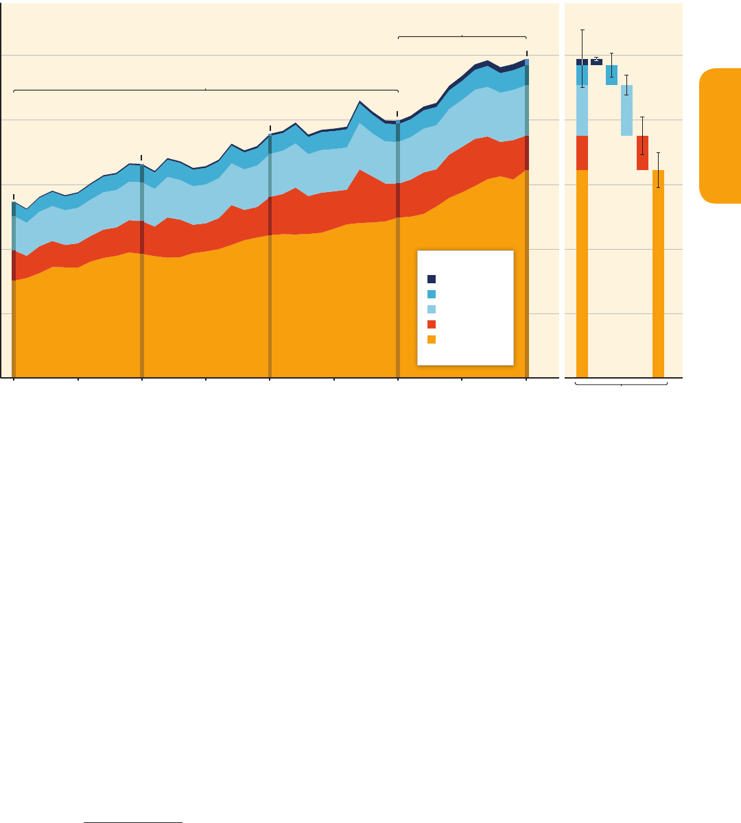
Figure SPM.1 | Total annual anthropogenic GHG emissions (GtCO
2
eq / yr) by groups of gases 1970 – 2010: CO
2
from fossil fuel combustion and industrial processes; CO
2
from
Forestry and Other Land Use (FOLU); methane (CH
4
); nitrous oxide (N
2
O); fluorinated gases
8
covered under the Kyoto Protocol (F-gases). At the right side of the figure GHG emis-
sions in 2010 are shown again broken down into these components with the associated uncertainties (90 % confidence interval) indicated by the error bars. Total anthropogenic
GHG emissions uncertainties are derived from the individual gas estimates as described in Chapter 5 [5.2.3.6]. Global CO
2
emissions from fossil fuel combustion are known within
8 % uncertainty (90 % confidence interval). CO
2
emissions from FOLU have very large uncertainties attached in the order of ± 50 %. Uncertainty for global emissions of CH
4
, N
2
O
and the F-gases has been estimated as 20 %, 60 % and 20 %, respectively. 2010 was the most recent year for which emission statistics on all gases as well as assessment of
uncertainties were essentially complete at the time of data cut-off for this report. Emissions are converted into CO
2
-equivalents based on GWP
100
6
from the IPCC Second Assessment
Report. The emission data from FOLU represents land-based CO
2
emissions from forest fires, peat fires and peat decay that approximate to net CO
2
flux from FOLU as described in
Chapter 11 of this report. Average annual growth rate over different periods is highlighted with the brackets. [Figure 1.3, Figure TS.1]
27 Gt
33 Gt
55%
17%
19%
7.9%
0.44%
58%
15%
18%
7.9%
0.67%
62%
13%
16%
6.9%
1.3%
38 Gt
40 Gt
59%
16%
18%
7.4%
0.81%
49 Gt
65%
11%
16%
6.2%
2.0%
2005
Gas
CO
2
Fossil Fuel and
Industrial Processes
CO
2
FOLU
CH
4
N
2
O
F-Gases
GHG Emissions [GtCO
2
eq/yr]
0
10
20
30
40
50
2010200520001995199019851980
19751970
+2.2%/yr
2000 – 2010
+1.3%/yr
1970 – 2000
2010
Total Annual Anthropogenic GHG Emissions by Groups of Gases 1970 – 2010

8
SPM
Summary for Policymakers
24 % (12 GtCO
2
eq, net emissions) in AFOLU, 21 % (10 GtCO
2
eq) in industry, 14 % (7.0 GtCO
2
eq) in transport and 6.4 %
(3.2 GtCO
2
eq) in buildings. When emissions from electricity and heat production are attributed to the sectors that use
the final energy (i. e. indirect emissions), the shares of the industry and buildings sectors in global GHG emissions are
increased to 31 % and 19 %
7
, respectively (Figure SPM.2). [7.3, 8.2, 9.2, 10.3, 11.2]
Globally, economic and population growth continue to be the most important drivers of increases in CO
2
emissions from fossil fuel combustion. The contribution of population growth between 2000 and 2010
remained roughly identical to the previous three decades, while the contribution of economic growth has
risen sharply (high confidence). Between 2000 and 2010, both drivers outpaced emission reductions from improve-
ments in energy intensity (Figure SPM.3). Increased use of coal relative to other energy sources has reversed the
long-standing trend of gradual decarbonization of the world’s energy supply. [1.3, 5.3, 7.2, 14.3, TS.2.2]
Without additional efforts to reduce GHG emissions beyond those in place today, emissions growth is
expected to persist driven by growth in global population and economic activities. Baseline scenarios, those
without additional mitigation, result in global mean surface temperature increases in 2100 from 3.7 °C to
4.8 °C compared to pre-industrial levels
10
(range based on median climate response; the range is 2.5 °C to
7.8 °C when including climate uncertainty, see Table SPM.1)
11
(high confidence). The emission scenarios collected for
this assessment represent full radiative forcing including GHGs, tropospheric ozone, aerosols and albedo change. Baseline
scenarios (scenarios without explicit additional efforts to constrain emissions) exceed 450 parts per million (ppm) CO
2
eq
by 2030 and reach CO
2
eq concentration levels between 750 and more than 1300 ppm CO
2
eq by 2100. This is similar to
the range in atmospheric concentration levels between the RCP 6.0 and RCP 8.5 pathways in 2100.
12
For comparison, the
CO
2
eq concentration in 2011 is estimated to be 430 ppm (uncertainty range 340 – 520 ppm).
13
[6.3, Box TS.6; WGI Figure
SPM.5, WGI 8.5, WGI 12.3]
10
Based on the longest global surface temperature dataset available, the observed change between the average of the period 1850 – 1900 and of
the AR5 reference period (1986 – 2005) is 0.61 °C (5 – 95 % confidence interval: 0.55 – 0.67 °C) [WGI SPM.E], which is used here as an approxi-
mation of the change in global mean surface temperature since pre-industrial times, referred to as the period before 1750.
11
The climate uncertainty reflects the 5th to 95th percentile of climate model calculations described in Table SPM.1.
12
For the purpose of this assessment, roughly 300 baseline scenarios and 900 mitigation scenarios were collected through an open call from
integrated modelling teams around the world. These scenarios are complementary to the Representative Concentration Pathways (RCPs, see
WGIII
AR5 Glossary). The RCPs are identified by their approximate total radiative forcing in year 2100 relative to 1750: 2.6 Watts per square meter
(
W /
m
2
) for RCP2.6, 4.5 W / m
2
for RCP4.5, 6.0 W / m
2
for RCP6.0, and 8.5 W /
m
2
for RCP8.5. The scenarios collected for this assessment span a
slightly broader range of concentrations in the year 2100 than the four RCPs.
13
This is based on the assessment of total anthropogenic radiative forcing for 2011 relative to 1750 in WGI, i. e. 2.3 W /
m
2
, uncertainty range 1.1 to
3.3 W /
m
2
. [WGI Figure SPM.5, WGI 8.5, WGI 12.3]
Figure SPM.2 | Total anthropogenic GHG emissions (GtCO
2
eq / yr) by economic sectors. Inner circle shows direct GHG emission shares (in % of total anthropogenic GHG emissions)
of five economic sectors in 2010. Pull-out shows how indirect CO
2
emission shares (in % of total anthropogenic GHG emissions) from electricity and heat production are attributed
to sectors of final energy use. ‘Other Energy’ refers to all GHG emission sources in the energy sector as defined in Annex II other than electricity and heat production [A.II.9.1]. The
emissions data from Agriculture, Forestry and Other Land Use (AFOLU) includes land-based CO
2
emissions from forest fires, peat fires and peat decay that approximate to net CO
2
flux from the Forestry and Other Land Use (FOLU) sub-sector as described in Chapter 11 of this report. Emissions are converted into CO
2
-equivalents based on GWP
100
6
from the
IPCC Second Assessment Report. Sector definitions are provided in Annex II.9. [Figure 1.3a, Figure TS.3 upper panel]
Greenhouse Gas Emissions by Economic Sectors
Indirect CO
2
Emissions
Direct Emissions
Buildings
6.4%
Transport
14%
Industry
21%
Other
Energy
9.6%
Electricity
and Heat Production
25%
49 Gt CO
2
eq
(2010)
AFOLU
24%
Buildings
12%
Transport
0.3%
Industry
11%
Energy
1.4%
AFOLU
0.87%
Figure SPM.3 | Decomposition of the change in total annual CO
2
emissions from fossil fuel combustion by decade and four driving factors: population, income (GDP) per capita,
energy intensity of GDP and carbon intensity of energy. The bar segments show the changes associated with each factor alone, holding the respective other factors constant. Total
emissions changes are indicated by a triangle. The change in emissions over each decade is measured in gigatonnes of CO
2
per year [GtCO
2
/ yr]; income is converted into common
units using purchasing power parities. [Figure 1.7]
1970-1980 1980-1990 1990-2000 2000-2010
-6
-4
-2
0
2
4
6
8
10
12
Change in Annual CO
2
Emissions by Decade [GtCO
2
/yr]
CarbonIntensity of Energy
EnergyIntensity of GDP
GDPperCapita
Population
TotalChange
6.8
2.5
2.9
4.0
Decomposition of the Change in Total Annual CO
2
Emissions from Fossil Fuel Combustion by Decade

9
SPM
Summary for Policymakers
24 % (12 GtCO
2
eq, net emissions) in AFOLU, 21 % (10 GtCO
2
eq) in industry, 14 % (7.0 GtCO
2
eq) in transport and 6.4 %
(3.2 GtCO
2
eq) in buildings. When emissions from electricity and heat production are attributed to the sectors that use
the final energy (i. e. indirect emissions), the shares of the industry and buildings sectors in global GHG emissions are
increased to 31 % and 19 %
7
, respectively (Figure SPM.2). [7.3, 8.2, 9.2, 10.3, 11.2]
Globally, economic and population growth continue to be the most important drivers of increases in CO
2
emissions from fossil fuel combustion. The contribution of population growth between 2000 and 2010
remained roughly identical to the previous three decades, while the contribution of economic growth has
risen sharply (high confidence). Between 2000 and 2010, both drivers outpaced emission reductions from improve-
ments in energy intensity (Figure SPM.3). Increased use of coal relative to other energy sources has reversed the
long-standing trend of gradual decarbonization of the world’s energy supply. [1.3, 5.3, 7.2, 14.3, TS.2.2]
Without additional efforts to reduce GHG emissions beyond those in place today, emissions growth is
expected to persist driven by growth in global population and economic activities. Baseline scenarios, those
without additional mitigation, result in global mean surface temperature increases in 2100 from 3.7 °C to
4.8 °C compared to pre-industrial levels
10
(range based on median climate response; the range is 2.5 °C to
7.8 °C when including climate uncertainty, see Table SPM.1)
11
(high confidence). The emission scenarios collected for
this assessment represent full radiative forcing including GHGs, tropospheric ozone, aerosols and albedo change. Baseline
scenarios (scenarios without explicit additional efforts to constrain emissions) exceed 450 parts per million (ppm) CO
2
eq
by 2030 and reach CO
2
eq concentration levels between 750 and more than 1300 ppm CO
2
eq by 2100. This is similar to
the range in atmospheric concentration levels between the RCP 6.0 and RCP 8.5 pathways in 2100.
12
For comparison, the
CO
2
eq concentration in 2011 is estimated to be 430 ppm (uncertainty range 340 – 520 ppm).
13
[6.3, Box TS.6; WGI Figure
SPM.5, WGI 8.5, WGI 12.3]
10
Based on the longest global surface temperature dataset available, the observed change between the average of the period 1850 – 1900 and of
the AR5 reference period (1986 – 2005) is 0.61 °C (5 – 95 % confidence interval: 0.55 – 0.67 °C) [WGI SPM.E], which is used here as an approxi-
mation of the change in global mean surface temperature since pre-industrial times, referred to as the period before 1750.
11
The climate uncertainty reflects the 5th to 95th percentile of climate model calculations described in Table SPM.1.
12
For the purpose of this assessment, roughly 300 baseline scenarios and 900 mitigation scenarios were collected through an open call from
integrated modelling teams around the world. These scenarios are complementary to the Representative Concentration Pathways (RCPs, see
WGIII
AR5 Glossary). The RCPs are identified by their approximate total radiative forcing in year 2100 relative to 1750: 2.6 Watts per square meter
(
W /
m
2
) for RCP2.6, 4.5 W / m
2
for RCP4.5, 6.0 W / m
2
for RCP6.0, and 8.5 W /
m
2
for RCP8.5. The scenarios collected for this assessment span a
slightly broader range of concentrations in the year 2100 than the four RCPs.
13
This is based on the assessment of total anthropogenic radiative forcing for 2011 relative to 1750 in WGI, i. e. 2.3 W /
m
2
, uncertainty range 1.1 to
3.3 W /
m
2
. [WGI Figure SPM.5, WGI 8.5, WGI 12.3]
Figure SPM.2 | Total anthropogenic GHG emissions (GtCO
2
eq / yr) by economic sectors. Inner circle shows direct GHG emission shares (in % of total anthropogenic GHG emissions)
of five economic sectors in 2010. Pull-out shows how indirect CO
2
emission shares (in % of total anthropogenic GHG emissions) from electricity and heat production are attributed
to sectors of final energy use. ‘Other Energy’ refers to all GHG emission sources in the energy sector as defined in Annex II other than electricity and heat production [A.II.9.1]. The
emissions data from Agriculture, Forestry and Other Land Use (AFOLU) includes land-based CO
2
emissions from forest fires, peat fires and peat decay that approximate to net CO
2
flux from the Forestry and Other Land Use (FOLU) sub-sector as described in Chapter 11 of this report. Emissions are converted into CO
2
-equivalents based on GWP
100
6
from the
IPCC Second Assessment Report. Sector definitions are provided in Annex II.9. [Figure 1.3a, Figure TS.3 upper panel]
Greenhouse Gas Emissions by Economic Sectors
Indirect CO
2
Emissions
Direct Emissions
Buildings
6.4%
Transport
14%
Industry
21%
Other
Energy
9.6%
Electricity
and Heat Production
25%
49 Gt CO
2
eq
(2010)
AFOLU
24%
Buildings
12%
Transport
0.3%
Industry
11%
Energy
1.4%
AFOLU
0.87%
Figure SPM.3 | Decomposition of the change in total annual CO
2
emissions from fossil fuel combustion by decade and four driving factors: population, income (GDP) per capita,
energy intensity of GDP and carbon intensity of energy. The bar segments show the changes associated with each factor alone, holding the respective other factors constant. Total
emissions changes are indicated by a triangle. The change in emissions over each decade is measured in gigatonnes of CO
2
per year [GtCO
2
/ yr]; income is converted into common
units using purchasing power parities. [Figure 1.7]
1970-1980 1980-1990 1990-2000 2000-2010
-6
-4
-2
0
2
4
6
8
10
12
Change in Annual CO
2
Emissions by Decade [GtCO
2
/yr]
CarbonIntensity of Energy
EnergyIntensity of GDP
GDPperCapita
Population
TotalChange
6.8
2.5
2.9
4.0
Decomposition of the Change in Total Annual CO
2
Emissions from Fossil Fuel Combustion by Decade

10
SPM
Summary for Policymakers
Mitigation pathways and measures in the context
of sustainable development
Long-term mitigation pathways
There are multiple scenarios with a range of technological and behavioral options, with different characteristics
and implications for sustainable development, that are consistent with different levels of mitigation. For this
assessment, about 900 mitigation scenarios have been collected in a database based on published integrated models.
14
This
range spans atmospheric concentration levels in 2100 from 430 ppm CO
2
eq to above 720 ppm CO
2
eq, which is comparable
to the 2100 forcing levels between RCP 2.6 and RCP 6.0. Scenarios outside this range were also assessed including some
scenarios with concentrations in 2100 below 430 ppm CO
2
eq (for a discussion of these scenarios see below). The mitigation
scenarios involve a wide range of technological, socioeconomic, and institutional trajectories, but uncertainties and model
limitations exist and developments outside this range are possible (Figure SPM.4, upper panel).
[6.1, 6.2, 6.3, TS.3.1, Box TS.6]
Mitigation scenarios in which it is likely that the temperature change caused by anthropogenic GHG emis-
sions can be kept to less than 2 °C relative to pre-industrial levels are characterized by atmospheric concen-
trations in 2100 of about 450 ppm CO
2
eq (high confidence). Mitigation scenarios reaching concentration levels of
about 500 ppm CO
2
eq by 2100 are more likely than not to limit temperature change to less than 2 °C relative to
pre-industrial levels, unless they temporarily ‘overshoot’ concentration levels of roughly 530 ppm CO
2
eq before 2100, in
which case they are about as likely as not to achieve that goal.
15
Scenarios that reach 530 to 650 ppm CO
2
eq concentra-
tions by 2100 are more unlikely than likely to keep temperature change below 2 °C relative to pre-industrial levels.
Scenarios that exceed about 650 ppm CO
2
eq by 2100 are unlikely to limit temperature change to below 2 °C relative to
pre-industrial levels. Mitigation scenarios in which temperature increase is more likely than not to be less than 1.5 °C
relative to pre-industrial levels by 2100 are characterized by concentrations in 2100 of below 430 ppm CO
2
eq. Tempera-
ture peaks during the century and then declines in these scenarios. Probability statements regarding other levels of
temperature change can be made with reference to Table SPM.1. [6.3, Box TS.6]
Scenarios reaching atmospheric concentration levels of about 450 ppm CO
2
eq by 2100 (consistent with a
likely chance to keep temperature change below 2 °C relative to pre-industrial levels) include substantial cuts
in anthropogenic GHG emissions by mid-century through large-scale changes in energy systems and poten-
tially land use (high confidence). Scenarios reaching these concentrations by 2100 are characterized by lower global
GHG emissions in 2050 than in 2010, 40 % to 70 % lower globally,
16
and emissions levels near zero GtCO
2
eq or below in
14
The long-term scenarios assessed in WGIII were generated primarily by large-scale, integrated models that project many key characteristics of
mitigation pathways to mid-century and beyond. These models link many important human systems (e. g., energy, agriculture and land use,
economy) with physical processes associated with climate change (e. g., the carbon cycle). The models approximate cost-effective solutions that
minimize the aggregate economic costs of achieving mitigation outcomes, unless they are specifically constrained to behave otherwise. They are
simplified, stylized representations of highly-complex, real-world processes, and the scenarios they produce are based on uncertain projections
about key events and drivers over often century-long timescales. Simplifications and differences in assumptions are the reason why output gen-
erated from different models, or versions of the same model, can differ, and projections from all models can differ considerably from the reality
that unfolds. [Box TS.7, 6.2]
15
Mitigation scenarios, including those reaching 2100 concentrations as high as or higher than about 550 ppm CO
2
eq, can temporarily ‘overshoot’
atmospheric CO
2
eq concentration levels before descending to lower levels later. Such concentration overshoot involves less mitigation in the near
term with more rapid and deeper emissions reductions in the long run. Overshoot increases the probability of exceeding any given temperature
goal. [6.3, Table SPM.1]
16
This range differs from the range provided for a similar concentration category in AR4 (50 % – 85 % lower than 2000 for CO
2
only). Reasons for
this difference include that this report has assessed a substantially larger number of scenarios than in AR4 and looks at all GHGs. In addition, a
large proportion of the new scenarios include Carbon Dioxide Removal (CDR) technologies (see below). Other factors include the use of 2100
concentration levels instead of stabilization levels and the shift in reference year from 2000 to 2010. Scenarios with higher emissions in 2050 are
characterized by a greater reliance on CDR technologies beyond mid-century.
SPM.4
SPM.4.1
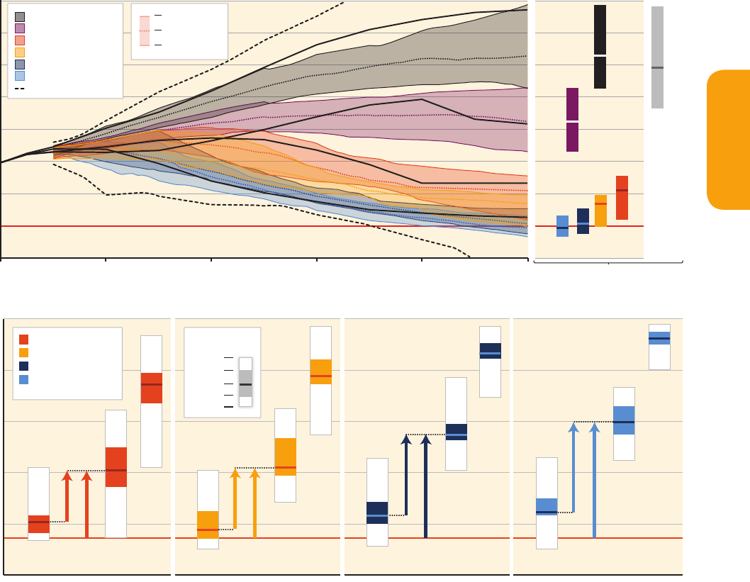
Figure SPM.4 | Pathways of global GHG emissions (GtCO
2
eq / yr) in baseline and mitigation scenarios for different long-term concentration levels (upper panel) [Figure 6.7] and
associated upscaling requirements of low-carbon energy (% of primary energy) for 2030, 2050 and 2100 compared to 2010 levels in mitigation scenarios (lower panel) [Figure
7.16]. The lower panel excludes scenarios with limited technology availability and exogenous carbon price trajectories. For definitions of CO
2
-equivalent emissions and CO
2
-equiva-
lent concentrations see the WGIII
AR5
Glossary.
21002000 2020 2040 2060 2080 2100
-20
0
20
40
60
80
100
120
140
Baseline
RCP8.5
RCP6.0
RCP4.5
RCP2.6
Associated Upscaling of Low-Carbon Energy Supply
0
20
40
60
80
100
2030 2050 2100 2030 2050 2100 2030 2050 2100 2030 2050 2100
Low-Carbon Energy Share of Primary Energy [%]
Annual GHG Emissions [GtCO
2
eq/yr]
> 1000
720 - 1000
580 - 720
530 - 580
480 - 530
430 - 480
Full AR5 Database Range
ppm CO
2
eq
ppm CO
2
eq
ppm CO
2
eq
ppm CO
2
eq
ppm CO
2
eq
ppm CO
2
eq
GHG Emission Pathways 2000-2100: All AR5 Scenarios
90
th
Percentile
Median
10
th
Percentile
580 - 720
530 - 580
480 - 530
430 - 480
ppm CO
2
eq
ppm CO
2
eq
ppm CO
2
eq
ppm CO
2
eq
Min
75
th
Max
Median
25
th
Percentile
+180%
+185%
+275%
+310%
+95%
+135%
+135%
+145%
2010
11
SPM
Summary for Policymakers
Mitigation pathways and measures in the context
of sustainable development
Long-term mitigation pathways
There are multiple scenarios with a range of technological and behavioral options, with different characteristics
and implications for sustainable development, that are consistent with different levels of mitigation. For this
assessment, about 900 mitigation scenarios have been collected in a database based on published integrated models.
14
This
range spans atmospheric concentration levels in 2100 from 430 ppm CO
2
eq to above 720 ppm CO
2
eq, which is comparable
to the 2100 forcing levels between RCP 2.6 and RCP 6.0. Scenarios outside this range were also assessed including some
scenarios with concentrations in 2100 below 430 ppm CO
2
eq (for a discussion of these scenarios see below). The mitigation
scenarios involve a wide range of technological, socioeconomic, and institutional trajectories, but uncertainties and model
limitations exist and developments outside this range are possible (Figure SPM.4, upper panel).
[6.1, 6.2, 6.3, TS.3.1, Box TS.6]
Mitigation scenarios in which it is likely that the temperature change caused by anthropogenic GHG emis-
sions can be kept to less than 2 °C relative to pre-industrial levels are characterized by atmospheric concen-
trations in 2100 of about 450 ppm CO
2
eq (high confidence). Mitigation scenarios reaching concentration levels of
about 500 ppm CO
2
eq by 2100 are more likely than not to limit temperature change to less than 2 °C relative to
pre-industrial levels, unless they temporarily ‘overshoot’ concentration levels of roughly 530 ppm CO
2
eq before 2100, in
which case they are about as likely as not to achieve that goal.
15
Scenarios that reach 530 to 650 ppm CO
2
eq concentra-
tions by 2100 are more unlikely than likely to keep temperature change below 2 °C relative to pre-industrial levels.
Scenarios that exceed about 650 ppm CO
2
eq by 2100 are unlikely to limit temperature change to below 2 °C relative to
pre-industrial levels. Mitigation scenarios in which temperature increase is more likely than not to be less than 1.5 °C
relative to pre-industrial levels by 2100 are characterized by concentrations in 2100 of below 430 ppm CO
2
eq. Tempera-
ture peaks during the century and then declines in these scenarios. Probability statements regarding other levels of
temperature change can be made with reference to Table SPM.1. [6.3, Box TS.6]
Scenarios reaching atmospheric concentration levels of about 450 ppm CO
2
eq by 2100 (consistent with a
likely chance to keep temperature change below 2 °C relative to pre-industrial levels) include substantial cuts
in anthropogenic GHG emissions by mid-century through large-scale changes in energy systems and poten-
tially land use (high confidence). Scenarios reaching these concentrations by 2100 are characterized by lower global
GHG emissions in 2050 than in 2010, 40 % to 70 % lower globally,
16
and emissions levels near zero GtCO
2
eq or below in
14
The long-term scenarios assessed in WGIII were generated primarily by large-scale, integrated models that project many key characteristics of
mitigation pathways to mid-century and beyond. These models link many important human systems (e. g., energy, agriculture and land use,
economy) with physical processes associated with climate change (e. g., the carbon cycle). The models approximate cost-effective solutions that
minimize the aggregate economic costs of achieving mitigation outcomes, unless they are specifically constrained to behave otherwise. They are
simplified, stylized representations of highly-complex, real-world processes, and the scenarios they produce are based on uncertain projections
about key events and drivers over often century-long timescales. Simplifications and differences in assumptions are the reason why output gen-
erated from different models, or versions of the same model, can differ, and projections from all models can differ considerably from the reality
that unfolds. [Box TS.7, 6.2]
15
Mitigation scenarios, including those reaching 2100 concentrations as high as or higher than about 550 ppm CO
2
eq, can temporarily ‘overshoot’
atmospheric CO
2
eq concentration levels before descending to lower levels later. Such concentration overshoot involves less mitigation in the near
term with more rapid and deeper emissions reductions in the long run. Overshoot increases the probability of exceeding any given temperature
goal. [6.3, Table SPM.1]
16
This range differs from the range provided for a similar concentration category in AR4 (50 % – 85 % lower than 2000 for CO
2
only). Reasons for
this difference include that this report has assessed a substantially larger number of scenarios than in AR4 and looks at all GHGs. In addition, a
large proportion of the new scenarios include Carbon Dioxide Removal (CDR) technologies (see below). Other factors include the use of 2100
concentration levels instead of stabilization levels and the shift in reference year from 2000 to 2010. Scenarios with higher emissions in 2050 are
characterized by a greater reliance on CDR technologies beyond mid-century.
SPM.4
SPM.4.1
Figure SPM.4 | Pathways of global GHG emissions (GtCO
2
eq / yr) in baseline and mitigation scenarios for different long-term concentration levels (upper panel) [Figure 6.7] and
associated upscaling requirements of low-carbon energy (% of primary energy) for 2030, 2050 and 2100 compared to 2010 levels in mitigation scenarios (lower panel) [Figure
7.16]. The lower panel excludes scenarios with limited technology availability and exogenous carbon price trajectories. For definitions of CO
2
-equivalent emissions and CO
2
-equiva-
lent concentrations see the WGIII
AR5
Glossary.
21002000 2020 2040 2060 2080 2100
-20
0
20
40
60
80
100
120
140
Baseline
RCP8.5
RCP6.0
RCP4.5
RCP2.6
Associated Upscaling of Low-Carbon Energy Supply
0
20
40
60
80
100
2030 2050 2100 2030 2050 2100 2030 2050 2100 2030 2050 2100
Low-Carbon Energy Share of Primary Energy [%]
Annual GHG Emissions [GtCO
2
eq/yr]
> 1000
720 - 1000
580 - 720
530 - 580
480 - 530
430 - 480
Full AR5 Database Range
ppm CO
2
eq
ppm CO
2
eq
ppm CO
2
eq
ppm CO
2
eq
ppm CO
2
eq
ppm CO
2
eq
GHG Emission Pathways 2000-2100: All AR5 Scenarios
90
th
Percentile
Median
10
th
Percentile
580 - 720
530 - 580
480 - 530
430 - 480
ppm CO
2
eq
ppm CO
2
eq
ppm CO
2
eq
ppm CO
2
eq
Min
75
th
Max
Median
25
th
Percentile
+180%
+185%
+275%
+310%
+95%
+135%
+135%
+145%
2010

12
SPM
Summary for Policymakers
2100. In scenarios reaching about 500 ppm CO
2
eq by 2100, 2050 emissions levels are 25 % to 55 % lower than in 2010
globally. In scenarios reaching about 550 ppm CO
2
eq, emissions in 2050 are from 5 % above 2010 levels to 45 % below
2010 levels globally (Table SPM.1). At the global level, scenarios reaching about 450 ppm CO
2
eq are also characterized
by more rapid improvements in energy efficiency and a tripling to nearly a quadrupling of the share of zero- and low-
carbon energy supply from renewables, nuclear energy and fossil energy with carbon dioxide capture and storage (CCS),
or bioenergy with CCS (BECCS) by the year 2050 (Figure SPM.4, lower panel). These scenarios describe a wide range of
changes in land use, reflecting different assumptions about the scale of bioenergy production, afforestation, and reduced
deforestation. All of these emissions, energy, and land-use changes vary across regions.
17
Scenarios reaching higher
concentrations include similar changes, but on a slower timescale. On the other hand, scenarios reaching lower concen-
trations require these changes on a faster timescale. [6.3, 7.11]
Mitigation scenarios reaching about 450 ppm CO
2
eq in 2100 typically involve temporary overshoot of
atmospheric concentrations, as do many scenarios reaching about 500 ppm to about 550 ppm CO
2
eq in 2100.
Depending on the level of the overshoot, overshoot scenarios typically rely on the availability and wide-
spread deployment of BECCS and afforestation in the second half of the century. The availability and scale of
these and other Carbon Dioxide Removal (CDR) technologies and methods are uncertain and CDR technolo-
gies and methods are, to varying degrees, associated with challenges and risks (high confidence) (see Section
SPM.4.2).
18
CDR is also prevalent in many scenarios without overshoot to compensate for residual emissions from sectors
where mitigation is more expensive. There is uncertainty about the potential for large-scale deployment of BECCS, large-
scale afforestation, and other CDR technologies and methods. [2.6, 6.3, 6.9.1, Figure 6.7, 7.11, 11.13]
Estimated global GHG emissions levels in 2020 based on the Cancún Pledges are not consistent with cost-
effective long-term mitigation trajectories that are at least about as likely as not to limit temperature
change to 2 °C relative to pre-industrial levels (2100 concentrations of about 450 to about 500 ppm CO
2
eq),
but they do not preclude the option to meet that goal (high confidence). Meeting this goal would require further
substantial reductions beyond 2020. The Cancún Pledges are broadly consistent with cost-effective scenarios that are
likely to keep temperature change below 3 °C relative to preindustrial levels. [6.4, 13.13, Figure TS.11]
Delaying mitigation efforts beyond those in place today through 2030 is estimated to substantially increase
the difficulty of the transition to low longer-term emissions levels and narrow the range of options consis-
tent with maintaining temperature change below 2 °C relative to pre-industrial levels (high confidence). Cost-
effective mitigation scenarios that make it at least about as likely as not that temperature change will remain below 2 °C
relative to pre-industrial levels (2100 concentrations of about 450 to about 500 ppm CO
2
eq) are typically characterized
by annual GHG emissions in 2030 of roughly between 30 GtCO
2
eq and 50 GtCO
2
eq (Figure SPM.5, left panel). Scenarios
with annual GHG emissions above 55 GtCO
2
eq in 2030 are characterized by substantially higher rates of emissions
reductions from 2030 to 2050 (Figure SPM.5, middle panel); much more rapid scale-up of low-carbon energy over this
period (FigureSPM.5, right panel); a larger reliance on CDR technologies in the long-term; and higher transitional and
long-term economic impacts (Table SPM.2, orange segment). Due to these increased mitigation challenges, many models
with annual 2030 GHG emissions higher than 55 GtCO
2
eq could not produce scenarios reaching atmospheric concentra-
tion levels that make it about as likely as not that temperature change will remain below 2 °C relative to pre-industrial
levels. [6.4, 7.11, Figures TS.11, TS.13]
17
At the national level, change is considered most effective when it reflects country and local visions and approaches to achieving sustainable
development according to national circumstances and priorities. [6.4, 11.8.4, WGII SPM]
18
According to WGI, CDR methods have biogeochemical and technological limitations to their potential on the global scale. There is insufficient
knowledge to quantify how much CO
2
emissions could be partially offset by CDR on a century timescale. CDR methods carry side-effects and
long-term consequences on a global scale. [WGI SPM.E.8]

13
SPM
Summary for Policymakers
Table SPM.1 | Key characteristics of the scenarios collected and assessed for WGIII AR5. For all parameters, the 10th to 90th percentile of the scenarios is shown.
1, 2
[Table 6.3]
CO
2
eq
Concentrations
in 2100 [ppm
CO
2
eq]
Category label
(concentration
range)
9
Subcategories
Relative
position of
the RCPs
5
Cumulative CO
2
emissions
3
[GtCO
2
]
Change in CO
2
eq emissions
compared to 2010 in [%]
4
Temperature change (relative to 1850 – 1900)
5, 6
2011 – 2050 2011 – 2100 2050 2100
2100
Temperature
change [°C]
7
Likelihood of staying below temperature
level over the 21st century
8
1.5 °C 2.0 °C 3.0 °C 4.0 °C
< 430 Only a limited number of individual model studies have explored levels below 430 ppm CO
2
eq
450
(430 – 480)
Total range
1, 10
RCP2.6 550 – 1300 630 – 1180 − 72 to − 41 − 118 to − 78
1.5 – 1.7
(1.0 – 2.8)
More unlikely
than likely
Likely
Likely
Likely
500
(480 – 530)
No overshoot of
530 ppm CO
2
eq
860 – 1180 960 – 1430 − 57 to − 42 − 107 to − 73
1.7 – 1.9
(1.2 – 2.9)
Unlikely
More likely
than not
Overshoot of
530 ppm CO
2
eq
1130 – 1530 990 – 1550 − 55 to − 25 − 114 to − 90
1.8 – 2.0
(1.2 – 3.3)
About as
likely as not
550
(530 – 580)
No overshoot of
580 ppm CO
2
eq
1070 – 1460 1240 – 2240 − 47 to − 19 − 81 to − 59
2.0 – 2.2
(1.4 – 3.6)
More unlikely
than likely
12
Overshoot of
580 ppm CO
2
eq
1420 – 1750 1170 – 2100 − 16 to 7 − 183 to − 86
2.1 – 2.3
(1.4 – 3.6)
(580 – 650) Total range
RCP4.5
1260 – 1640 1870 – 2440 − 38 to 24 − 134 to − 50
2.3 – 2.6
(1.5 – 4.2)
(650 – 720) Total range 1310 – 1750 2570 – 3340 − 11 to 17 − 54 to − 21
2.6 – 2.9
(1.8 – 4.5)
Unlikely
More likely
than not
(720 – 1000) Total range RCP6.0 1570 – 1940 3620 – 4990 18 to 54 − 7 to 72
3.1 – 3.7
(2.1 – 5.8)
Unlikely
11
More unlikely
than likely
> 1000 Total range RCP8.5 1840 – 2310 5350 – 7010 52 to 95 74 to 178
4.1 – 4.8
(2.8 – 7.8)
Unlikely
11
Unlikely
More unlikely
than likely
1
The ‘total range’ for the 430 – 480 ppm CO
2
eq scenarios corresponds to the range of the 10th – 90th percentile of the subcategory of these scenarios shown in Table 6.3.
2
Baseline scenarios (see SPM.3) fall into the > 1000 and 720 – 1000 ppm CO
2
eq categories. The latter category also includes mitigation scenarios. The baseline scenarios in the latter
category reach a temperature change of 2.5 – 5.8 °C above preindustrial in 2100. Together with the baseline scenarios in the > 1000 ppm CO
2
eq category, this leads to an overall 2100
temperature range of 2.5 – 7.8 °C (range based on median climate response: 3.7 – 4.8 °C) for baseline scenarios across both concentration categories.
3
For comparison of the cumulative CO
2
emissions estimates assessed here with those presented in WGI, an amount of 515 [445 – 585] GtC (1890 [1630 – 2150] GtCO
2
), was
already emitted by 2011 since 1870 [Section WGI 12.5]. Note that cumulative emissions are presented here for different periods of time (2011 – 2050 and 2011 – 2100) while
cumulative emissions in WGI are presented as total compatible emissions for the RCPs (2012 – 2100) or for total compatible emissions for remaining below a given tempera-
ture target with a given likelihood [WGI Table SPM.3, WGI SPM.E.8].
4
The global 2010 emissions are 31 % above the 1990 emissions (consistent with the historic GHG emission estimates presented in this report). CO
2
eq emissions include the
basket of Kyoto gases (CO
2
, CH
4
, N
2
O as well as F-gases).
5
The assessment in WGIII involves a large number of scenarios published in the scientific literature and is thus not limited to the RCPs. To evaluate the CO
2
eq concentration
and climate implications of these scenarios, the MAGICC model was used in a probabilistic mode (see AnnexII). For a comparison between MAGICC model results and
the outcomes of the models used in WGI, see Sections WGI 12.4.1.2 and WGI 12.4.8 and 6.3.2.6. Reasons for differences with WGI SPM Table.2 include the difference in
reference year (1986 – 2005 vs. 1850 – 1900 here), difference in reporting year (2081 – 2100 vs 2100 here), set-up of simulation (CMIP5 concentration driven versus MAGICC
emission-driven here), and the wider set of scenarios (RCPs versus the full set of scenarios in the WGIII AR5 scenario database here).
6
Temperature change is reported for the year 2100, which is not directly comparable to the equilibrium warming reported in WGIII AR4 [Table 3.5, Chapter 3]. For the 2100
temperature estimates, the transient climate response (TCR) is the most relevant system property. The assumed 90 % range of the TCR for MAGICC is 1.2 – 2.6 °C (median
1.8 °C). This compares to the 90 % range of TCR between 1.2 – 2.4 °C for CMIP5 [WGI 9.7] and an assessed likely range of 1 – 2.5 °C from multiple lines of evidence reported
in the WGI AR5 [Box 12.2 in Section 12.5].
7
Temperature change in 2100 is provided for a median estimate of the MAGICC calculations, which illustrates differences between the emissions pathways of the scenarios
in each category. The range of temperature change in the parentheses includes in addition the carbon cycle and climate system uncertainties as represented by the MAGICC
model [see 6.3.2.6 for further details]. The temperature data compared to the 1850 – 1900 reference year was calculated by taking all projected warming relative to
1986 – 2005, and adding 0.61 °C for 1986 – 2005 compared to 1850 – 1900, based on HadCRUT4 [see WGI Table SPM.2].
8
The assessment in this table is based on the probabilities calculated for the full ensemble of scenarios in WGIII using MAGICC and the assessment in WGI of the uncertainty
of the temperature projections not covered by climate models. The statements are therefore consistent with the statements in WGI, which are based on the CMIP5 runs of the
RCPs and the assessed uncertainties. Hence, the likelihood statements reflect different lines of evidence from both WGs. This WGI method was also applied for scenarios with
intermediate concentration levels where no CMIP5 runs are available. The likelihood statements are indicative only [6.3], and follow broadly the terms used by the WGI SPM
for temperature projections: likely 66 – 100 %, more likely than not > 50 – 100 %, about as likely as not 33 – 66 %, and unlikely 0 – 33 %. In addition the term more unlikely
than likely 0–< 50 % is used.
9
The CO
2
-equivalent concentration includes the forcing of all GHGs including halogenated gases and tropospheric ozone, as well as aerosols and albedo change (calculated on
the basis of the total forcing from a simple carbon cycle / climate model, MAGICC).
10
T he vast majority of scenarios in this category overshoot the category boundary of 480 ppm CO
2
eq concentrations.
11
For scenarios in this category no CMIP5 run [WGI Chapter 12, Table 12.3] as well as no MAGICC realization [6.3] stays below the respective temperature level. Still, an
unlikely assignment is given to reflect uncertainties that might not be reflected by the current climate models.
12
Scenarios in the 580 – 650 ppm CO
2
eq category include both overshoot scenarios and scenarios that do not exceed the concentration level at the high end of the category
(like RCP4.5). The latter type of scenarios, in general, have an assessed probability of more unlikely than likely to stay below the 2 °C temperature level, while the former are
mostly assessed to have an unlikely probability of staying below this level.
14
SPM
Summary for Policymakers
Estimates of the aggregate economic costs of mitigation vary widely and are highly sensitive to model design
and assumptions as well as the specification of scenarios, including the characterization of technologies and
the timing of mitigation (high confidence). Scenarios in which all countries of the world begin mitigation immediately,
there is a single global carbon price, and all key technologies are available, have been used as a cost-effective benchmark
for estimating macroeconomic mitigation costs (Table SPM.2, yellow segments). Under these assumptions, mitigation
scenarios that reach atmospheric concentrations of about 450 ppm CO
2
eq by 2100 entail losses in global consumption—
not including benefits of reduced climate change as well as co-benefits and adverse side-effects of mitigation
19
—of 1 % to
4 % (median: 1.7 %) in 2030, 2 % to 6 % (median: 3.4 %) in 2050, and 3 % to 11 % (median: 4.8 %) in 2100 relative to
consumption in baseline scenarios that grows anywhere from 300 % to more than 900 % over the century. These numbers
19
The total economic effect at different temperature levels would include mitigation costs, co-benefits of mitigation, adverse side-effects of mitiga-
tion, adaptation costs and climate damages. Mitigation cost and climate damage estimates at any given temperature level cannot be compared
to evaluate the costs and benefits of mitigation. Rather, the consideration of economic costs and benefits of mitigation should include the reduc-
tion of climate damages relative to the case of unabated climate change.
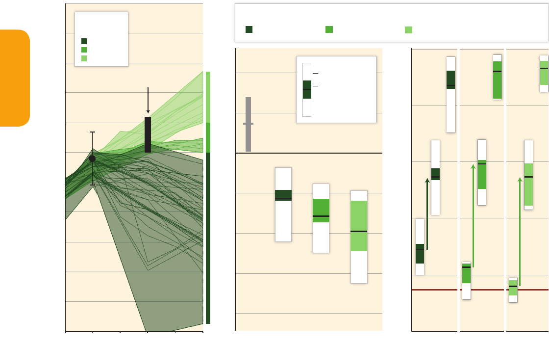
Figure SPM.5 | The implications of different 2030 GHG emissions levels (left panel) for the rate of CO
2
emissions reductions from 2030 to 2050 (middle panel) and low-carbon
energy upscaling from 2030 to 2050 and 2100 (right panel) in mitigation scenarios reaching about 450 to about 500 (430 – 530) ppm CO
2
eq concentrations by 2100. The scenarios
are grouped according to different emissions levels by 2030 (coloured in different shades of green). The left panel shows the pathways of GHG emissions (GtCO
2
eq / yr) leading to
these 2030 levels. The black bar shows the estimated uncertainty range of GHG emissions implied by the Cancún Pledges. The middle panel denotes the average annual CO
2
emis-
sions reduction rates for the period 2030 – 2050. It compares the median and interquartile range across scenarios from recent intermodel comparisons with explicit 2030 interim
goals to the range of scenarios in the Scenario Database for WGIII AR5. Annual rates of historical emissions change between 1900 – 2010 (sustained over a period of 20 years) and
average annual emissions change between 2000 – 2010 are shown in grey. The arrows in the right panel show the magnitude of zero and low-carbon energy supply up-scaling
from 2030 to 2050 subject to different 2030 GHG emissions levels. Zero- and low-carbon energy supply includes renewables, nuclear energy, fossil energy with carbon dioxide cap-
ture and storage (CCS), and bioenergy with CCS (BECCS). Note: Only scenarios that apply the full, unconstrained mitigation technology portfolio of the underlying models (default
technology assumption) are shown. Scenarios with large net negative global emissions (> 20 GtCO
2
/ yr), scenarios with exogenous carbon price assumptions, and scenarios with
2010 emissions significantly outside the historical range are excluded. The right-hand panel includes only 68 scenarios, because three of the 71 scenarios shown in the figure do not
report some subcategories for primary energy that are required to calculate the share of zero- and low-carbon energy. [Figures 6.32 and 7.16; 13.13.1.3]
+90%
+160%
+240%
2010
0
20
40
60
80
100
2030 2050 2100 2030 2050 2100 2030 2050
2100
Implications of Different 2030 GHG
Emissions Levels for Low-Carbon Energy
Upscaling
Zero- and Low-Carbon Energy Share of Primary Energy [%]
GHG Emissions Pathways to 2030 Implications of Different 2030 GHG Emissions
Levels for the Rate of Annual Average CO
2
Emissions Reductions from 2030 to 2050
Annual Rate of Change in CO
2
Emissions (2030 – 2050) [%/yr]
-12
-9
-6
-3
0
3
6
History
1900 – 2010
2000 – 2010
AR5 Scenario Range
Interquartile Range
and Median of Model
Comparisons with
2030 Targets
Annual GHG Emissions [GtCO
2
eq/yr]
<50 GtCO
2
eq
Annual GHG Emissions in 2030
50 – 5 5 GtCO
2
eq
>55 GtCO
2
eq
n=68n=71
Cancún
Pledges
<50 GtCO
2
eq
Annual
GHG Emissions
in 2030
50 – 55 GtCO
2
eq
>55 GtCO
2
eq
2005 2010 2015 2020 2025 2030
20
25
30
35
40
45
50
55
70
75
60
65
n=71

15
SPM
Summary for Policymakers
Estimates of the aggregate economic costs of mitigation vary widely and are highly sensitive to model design
and assumptions as well as the specification of scenarios, including the characterization of technologies and
the timing of mitigation (high confidence). Scenarios in which all countries of the world begin mitigation immediately,
there is a single global carbon price, and all key technologies are available, have been used as a cost-effective benchmark
for estimating macroeconomic mitigation costs (Table SPM.2, yellow segments). Under these assumptions, mitigation
scenarios that reach atmospheric concentrations of about 450 ppm CO
2
eq by 2100 entail losses in global consumption—
not including benefits of reduced climate change as well as co-benefits and adverse side-effects of mitigation
19
—of 1 % to
4 % (median: 1.7 %) in 2030, 2 % to 6 % (median: 3.4 %) in 2050, and 3 % to 11 % (median: 4.8 %) in 2100 relative to
consumption in baseline scenarios that grows anywhere from 300 % to more than 900 % over the century. These numbers
19
The total economic effect at different temperature levels would include mitigation costs, co-benefits of mitigation, adverse side-effects of mitiga-
tion, adaptation costs and climate damages. Mitigation cost and climate damage estimates at any given temperature level cannot be compared
to evaluate the costs and benefits of mitigation. Rather, the consideration of economic costs and benefits of mitigation should include the reduc-
tion of climate damages relative to the case of unabated climate change.
Figure SPM.5 | The implications of different 2030 GHG emissions levels (left panel) for the rate of CO
2
emissions reductions from 2030 to 2050 (middle panel) and low-carbon
energy upscaling from 2030 to 2050 and 2100 (right panel) in mitigation scenarios reaching about 450 to about 500 (430 – 530) ppm CO
2
eq concentrations by 2100. The scenarios
are grouped according to different emissions levels by 2030 (coloured in different shades of green). The left panel shows the pathways of GHG emissions (GtCO
2
eq / yr) leading to
these 2030 levels. The black bar shows the estimated uncertainty range of GHG emissions implied by the Cancún Pledges. The middle panel denotes the average annual CO
2
emis-
sions reduction rates for the period 2030 – 2050. It compares the median and interquartile range across scenarios from recent intermodel comparisons with explicit 2030 interim
goals to the range of scenarios in the Scenario Database for WGIII AR5. Annual rates of historical emissions change between 1900 – 2010 (sustained over a period of 20 years) and
average annual emissions change between 2000 – 2010 are shown in grey. The arrows in the right panel show the magnitude of zero and low-carbon energy supply up-scaling
from 2030 to 2050 subject to different 2030 GHG emissions levels. Zero- and low-carbon energy supply includes renewables, nuclear energy, fossil energy with carbon dioxide cap-
ture and storage (CCS), and bioenergy with CCS (BECCS). Note: Only scenarios that apply the full, unconstrained mitigation technology portfolio of the underlying models (default
technology assumption) are shown. Scenarios with large net negative global emissions (> 20 GtCO
2
/ yr), scenarios with exogenous carbon price assumptions, and scenarios with
2010 emissions significantly outside the historical range are excluded. The right-hand panel includes only 68 scenarios, because three of the 71 scenarios shown in the figure do not
report some subcategories for primary energy that are required to calculate the share of zero- and low-carbon energy. [Figures 6.32 and 7.16; 13.13.1.3]
+90%
+160%
+240%
2010
0
20
40
60
80
100
2030 2050 2100 2030 2050 2100 2030 2050 2100
Implications of Different 2030 GHG
Emissions Levels for Low-Carbon Energy
Upscaling
Zero- and Low-Carbon Energy Share of Primary Energy [%]
GHG Emissions Pathways to 2030 Implications of Different 2030 GHG Emissions
Levels for the Rate of Annual Average CO
2
Emissions Reductions from 2030 to 2050
Annual Rate of Change in CO
2
Emissions (2030 – 2050) [%/yr]
-12
-9
-6
-3
0
3
6
History
1900 – 2010
2000 – 2010
AR5 Scenario Range
Interquartile Range
and Median of Model
Comparisons with
2030 Targets
Annual GHG Emissions [GtCO
2
eq/yr]
<50 GtCO
2
eq
Annual GHG Emissions in 2030
50 – 5 5 GtCO
2
eq
>55 GtCO
2
eq
n=68n=71
Cancún
Pledges
<50 GtCO
2
eq
Annual
GHG Emissions
in 2030
50 – 55 GtCO
2
eq
>55 GtCO
2
eq
2005 2010 2015 2020 2025 2030
20
25
30
35
40
45
50
55
70
75
60
65
n=71
Table SPM.2 | Global mitigation costs in cost-effective scenarios
1
and estimated cost increases due to assumed limited availability of specific technologies and delayed additional
mitigation. Cost estimates shown in this table do not consider the benefits of reduced climate change as well as co-benefits and adverse side-effects of mitigation. The yellow col-
umns show consumption losses in the years 2030, 2050, and 2100 and annualized consumption growth reductions over the century in cost-effective scenarios relative to a baseline
development without climate policy. The grey columns show the percentage increase in discounted costs
2
over the century, relative to cost-effective scenarios, in scenarios in which
technology is constrained relative to default technology assumptions.
3
The orange columns show the increase in mitigation costs over the periods 2030 – 2050 and 2050 – 2100,
relative to scenarios with immediate mitigation, due to delayed additional mitigation through 2030.
4
These scenarios with delayed additional mitigation are grouped by emission
levels of less or more than 55 GtCO
2
eq in 2030, and two concentration ranges in 2100 (430 – 530 ppm CO
2
eq and 530 – 650 ppm CO
2
eq). In all figures, the median of the scenario
set is shown without parentheses, the range between the 16th and 84th percentile of the scenario set is shown in the parentheses, and the number of scenarios in the set is shown
in square brackets.
5
[Figures TS.12, TS.13, 6.21, 6.24, 6.25, Annex II.10]
Consumption losses in cost-effective scenarios
1
Increase in total discounted mitigation costs in
scenarios with limited availability of technologies
Increase in medium- and long-term mitigation costs
due to delayed additional mitigation until 2030
[% reduction in consumption
relative to baseline]
[percentage
point
reduction in
annualized
consumption
growth rate]
[% increase in total discounted mitigation costs
(2015 – 2100) relative to default technology assumptions]
[% increase in mitigation costs relative
to immediate mitigation]
2100
Concentration
[ppm CO
2
eq]
2030 2050 2100 2010 – 2100 No CCS
Nuclear
phase out
Limited
Solar / Wind
Limited
Bioenergy
≤ 55 GtCO
2
eq > 55 GtCO
2
eq
2030 – 2050 2050 – 2100 2030 – 2050 2050 – 2100
450 (430 – 480)
1.7
(1.0 – 3.7)
[N: 14]
3.4
(2.1 – 6.2)
4.8
(2.9 – 11.4)
0.06
(0.04 – 0.14)
138
(29 – 297)
[N: 4]
7
(4 – 18)
[N: 8]
6
(2 – 29)
[N: 8]
64
(44 – 78)
[N: 8]
28
(14 – 50)
[N: 34]
15
(5 – 59)
44
(2 – 78)
[N: 29]
37
(16 – 82)
500 (480 – 530)
1.7
(0.6 – 2.1)
[N: 32]
2.7
(1.5 – 4.2)
4.7
(2.4 – 10.6)
0.06
(0.03 – 0.13)
N / A N / A N / A N / A
550 (530 – 580)
0.6
(0.2 – 1.3)
[N: 46]
1.7
(1.2 – 3.3)
3.8
(1.2 – 7.3)
0.04
(0.01 – 0.09)
39
(18 – 78)
[N: 11]
13
(2 – 23)
[N: 10]
8
(5 – 15)
[N: 10]
18
(4 – 66)
[N: 12]
3
(− 5 – 16)
[N: 14]
4
(− 4 – 11)
15
(3 – 32)
[N: 10]
16
(5 – 24)
580 – 650
0.3
(0 – 0.9)
[N: 16]
1.3
(0.5 – 2.0)
2.3
(1.2 – 4.4)
0.03
(0.01 – 0.05)
N / A N / A N / A N / A
1
Cost-effective scenarios assume immediate mitigation in all countries and a single global carbon price, and impose no additional limitations on technology relative to the
models’ default technology assumptions.
2
Percentage increase of net present value of consumption losses in percent of baseline consumption (for scenarios from general equilibrium models) and abatement costs in
percent of baseline GDP (for scenarios from partial equilibrium models) for the period 2015 – 2100, discounted at 5 % per year.
3
No CCS: CCS is not included in these scenarios. Nuclear phase out: No addition of nuclear power plants beyond those under construction, and operation of existing plants
until the end of their lifetime. Limited Solar / Wind: a maximum of 20 % global electricity generation from solar and wind power in any year of these scenarios. Limited Bioen-
ergy: a maximum of 100 EJ / yr modern bioenergy supply globally (modern bioenergy used for heat, power, combinations, and industry was around 18 EJ / yr in 2008 [11.13.5]).
4
Percentage increase of total undiscounted mitigation costs for the periods 2030 – 2050 and 2050 – 2100.
5
The range is determined by the central scenarios encompassing the 16th and 84th percentile of the scenario set. Only scenarios with a time horizon until 2100 are included.
Some models that are included in the cost ranges for concentration levels above 530 ppm CO
2
eq in 2100 could not produce associated scenarios for concentration levels
below 530 ppm CO
2
eq in 2100 with assumptions about limited availability of technologies and / or delayed additional mitigation.
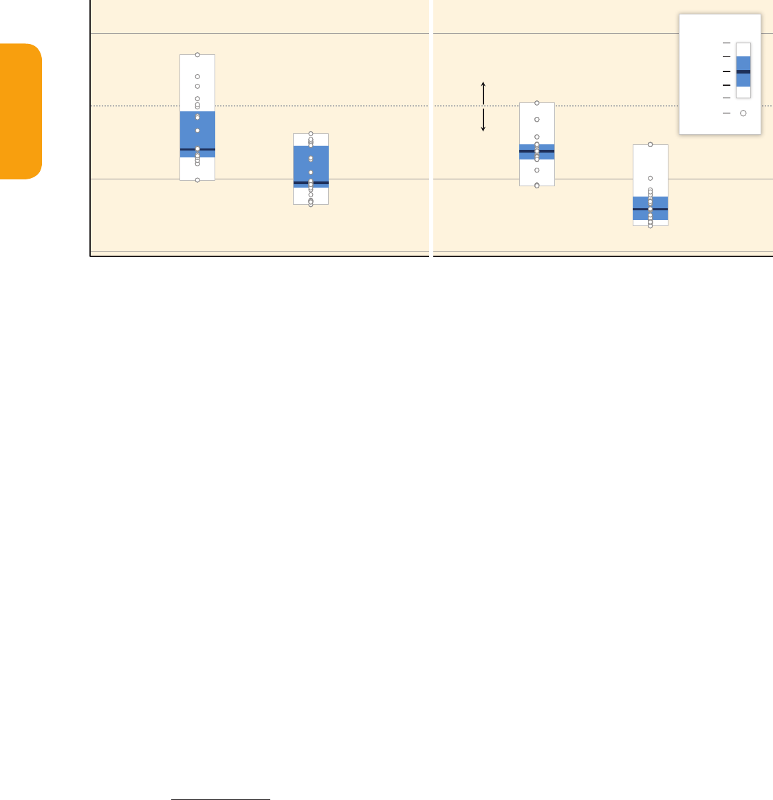
16
SPM
Summary for Policymakers
health and ecosystems associated with major cuts in air pollutant emissions (Figure SPM.6) are particularly high where
currently legislated and planned air pollution controls are weak. There is a wide range of co-benefits and adverse
side-effects for additional objectives other than air quality and energy security. Overall, the potential for co-benefits of
energy end-use measures outweighs the potential for adverse side-effects, whereas the evidence suggests this may not
be the case for all energy supply and AFOLU measures. [WGIII 4.8, 5.7, 6.3.6, 6.6, 7.9, 8.7, 9.7, 10.8, 11.7, 11.13.6, 12.8,
Figure TS.14, Table 6.7, Tables TS.3–TS.7; WGII 11.9]
There is a wide range of possible adverse side-effects as well as co-benefits and spillovers from climate
policy that have not been well-quantified (high confidence). Whether or not side-effects materialize, and to what
extent side-effects materialize, will be case- and site-specific, as they will depend on local circumstances and the scale,
scope, and pace of implementation. Important examples include biodiversity conservation, water availability, food
security, income distribution, efficiency of the taxation system, labour supply and employment, urban sprawl, and the
sustainability of the growth of developing countries. [Box TS.11]
Mitigation efforts and associated costs vary between countries in mitigation scenarios. The distribution of
costs across countries can differ from the distribution of the actions themselves (high confidence). In globally
cost-effective scenarios, the majority of mitigation efforts takes place in countries with the highest future emissions in
baseline scenarios. Some studies exploring particular effort-sharing frameworks, under the assumption of a global carbon
market, have estimated substantial global financial flows associated with mitigation for scenarios leading to 2100 atmo-
spheric concentrations of about 450 to about 550 ppm CO
2
eq. [4.6, 6.3.6, 13.4.2.4; Box 3.5; Table 6.4; Figures 6.9, 6.27,
6.28, 6.29]
Mitigation policy could devalue fossil fuel assets and reduce revenues for fossil fuel exporters, but differ-
ences between regions and fuels exist (high confidence). Most mitigation scenarios are associated with reduced
revenues from coal and oil trade for major exporters (high confidence). The effect of mitigation on natural gas export
revenues is more uncertain, with some studies showing possible benefits for export revenues in the medium term until
about 2050 (medium confidence). The availability of CCS would reduce the adverse effect of mitigation on the value of
fossil fuel assets (medium confidence). [6.3.6, 6.6, 14.4.2]
Sectoral and cross-sectoral mitigation pathways and measures
Cross-sectoral mitigation pathways and measures
In baseline scenarios, GHG emissions are projected to grow in all sectors, except for net CO
2
emissions in
the AFOLU sector
21
(robust evidence, medium agreement). Energy supply sector emissions are expected to continue
to be the major source of GHG emissions, ultimately accounting for the significant increases in indirect emissions from
electricity use in the buildings and industry sectors. In baseline scenarios, while non-CO
2
GHG agricultural emissions are
projected to increase, net CO
2
emissions from the AFOLU sector decline over time, with some models projecting a net sink
towards the end of the century (Figure SPM.7).
22
[6.3.1.4, 6.8, Figure TS.15]
21
Net AFOLU CO
2
emissions include emissions and removals of CO
2
from the AFOLU sector, including land under forestry and, in some assessments,
CO
2
sinks in agricultural soils.
22
A majority of the Earth System Models assessed in WGI project a continued land carbon uptake under all RCPs through to 2100, but some
models simulate a land carbon loss due to the combined effect of climate change and land-use change. [WGI SPM.E.7, WGI 6.4]
Figure SPM.6 | Air pollutant emission levels for black carbon (BC) and sulfur dioxide (SO
2
) in 2050 relative to 2005 (0=2005 levels). Baseline scenarios without additional efforts
to reduce GHG emissions beyond those in place today are compared to scenarios with stringent mitigation policies, which are consistent with reaching about 450 to about 500
(430– 530) ppm CO
2
eq concentrations by 2100. [Figure 6.33]
Individual
Scenarios
Min
75
th
Max
Median
25
th
Percentile
Stringent Climate Policy Stringent Climate PolicyBaseline Baseline
Change from 2005 [%]
Co-Benefits of Climate Change Mitigation for Air Quality
Impact of Stringent Climate Policy on Air Pollutant Emissions (Global, 2005-2050)
Increased
Pollution
Decreased
Pollution
-100
-50
0
50
Black Carbon Sulfur Dioxide
SPM.4.2
SPM.4.2.1
correspond to an annualized reduction of consumption growth by 0.04 to 0.14 (median: 0.06) percentage points over the
century relative to annualized consumption growth in the baseline that is between 1.6 % and 3 % per year. Estimates at
the high end of these cost ranges are from models that are relatively inflexible to achieve the deep emissions reductions
required in the long run to meet these goals and / or include assumptions about market imperfections that would raise
costs. Under the absence or limited availability of technologies, mitigation costs can increase substantially depending on
the technology considered (Table SPM.2, grey segment). Delaying additional mitigation further increases mitigation costs
in the medium- to long-term (Table SPM.2, orange segment). Many models could not achieve atmospheric concentration
levels of about 450 ppm CO
2
eq by 2100 if additional mitigation is considerably delayed or under limited availability of key
technologies, such as bioenergy, CCS, and their combination (BECCS). [6.3]
Only a limited number of studies have explored scenarios that are more likely than not to bring temperature
change back to below 1.5 °C by 2100 relative to pre-industrial levels; these scenarios bring atmospheric
concentrations to below 430 ppm CO
2
eq by 2100 (high confidence). Assessing this goal is currently difficult because
no multi-model studies have explored these scenarios. Scenarios associated with the limited number of published studies
exploring this goal are characterized by (1) immediate mitigation action; (2) the rapid upscaling of the full portfolio of
mitigation technologies; and (3) development along a low-energy demand trajectory.
20
[6.3, 7.11]
Mitigation scenarios reaching about 450 to about 500 ppm CO
2
eq by 2100 show reduced costs for achieving
air quality and energy security objectives, with significant co-benefits for human health, ecosystem impacts,
and sufficiency of resources and resilience of the energy system; these scenarios did not quantify other
co-benefits or adverse side-effects (medium confidence). These mitigation scenarios show improvements in terms of
the sufficiency of resources to meet national energy demand as well as the resilience of energy supply, resulting in
energy systems that are less vulnerable to price volatility and supply disruptions. The benefits from reduced impacts to
20
In these scenarios, the cumulative CO
2
emissions range between 680 and 800 GtCO
2
for the period 2011 – 2050 and between 90 and 310 GtCO
2
for the period 2011 – 2100. Global CO
2
eq emissions in 2050 are between 70 and 95 % below 2010 emissions, and they are between 110 and
120 % below 2010 emissions in 2100.

17
SPM
Summary for Policymakers
health and ecosystems associated with major cuts in air pollutant emissions (Figure SPM.6) are particularly high where
currently legislated and planned air pollution controls are weak. There is a wide range of co-benefits and adverse
side-effects for additional objectives other than air quality and energy security. Overall, the potential for co-benefits of
energy end-use measures outweighs the potential for adverse side-effects, whereas the evidence suggests this may not
be the case for all energy supply and AFOLU measures. [WGIII 4.8, 5.7, 6.3.6, 6.6, 7.9, 8.7, 9.7, 10.8, 11.7, 11.13.6, 12.8,
Figure TS.14, Table 6.7, Tables TS.3–TS.7; WGII 11.9]
There is a wide range of possible adverse side-effects as well as co-benefits and spillovers from climate
policy that have not been well-quantified (high confidence). Whether or not side-effects materialize, and to what
extent side-effects materialize, will be case- and site-specific, as they will depend on local circumstances and the scale,
scope, and pace of implementation. Important examples include biodiversity conservation, water availability, food
security, income distribution, efficiency of the taxation system, labour supply and employment, urban sprawl, and the
sustainability of the growth of developing countries. [Box TS.11]
Mitigation efforts and associated costs vary between countries in mitigation scenarios. The distribution of
costs across countries can differ from the distribution of the actions themselves (high confidence). In globally
cost-effective scenarios, the majority of mitigation efforts takes place in countries with the highest future emissions in
baseline scenarios. Some studies exploring particular effort-sharing frameworks, under the assumption of a global carbon
market, have estimated substantial global financial flows associated with mitigation for scenarios leading to 2100 atmo-
spheric concentrations of about 450 to about 550 ppm CO
2
eq. [4.6, 6.3.6, 13.4.2.4; Box 3.5; Table 6.4; Figures 6.9, 6.27,
6.28, 6.29]
Mitigation policy could devalue fossil fuel assets and reduce revenues for fossil fuel exporters, but differ-
ences between regions and fuels exist (high confidence). Most mitigation scenarios are associated with reduced
revenues from coal and oil trade for major exporters (high confidence). The effect of mitigation on natural gas export
revenues is more uncertain, with some studies showing possible benefits for export revenues in the medium term until
about 2050 (medium confidence). The availability of CCS would reduce the adverse effect of mitigation on the value of
fossil fuel assets (medium confidence). [6.3.6, 6.6, 14.4.2]
Sectoral and cross-sectoral mitigation pathways and measures
Cross-sectoral mitigation pathways and measures
In baseline scenarios, GHG emissions are projected to grow in all sectors, except for net CO
2
emissions in
the AFOLU sector
21
(robust evidence, medium agreement). Energy supply sector emissions are expected to continue
to be the major source of GHG emissions, ultimately accounting for the significant increases in indirect emissions from
electricity use in the buildings and industry sectors. In baseline scenarios, while non-CO
2
GHG agricultural emissions are
projected to increase, net CO
2
emissions from the AFOLU sector decline over time, with some models projecting a net sink
towards the end of the century (Figure SPM.7).
22
[6.3.1.4, 6.8, Figure TS.15]
21
Net AFOLU CO
2
emissions include emissions and removals of CO
2
from the AFOLU sector, including land under forestry and, in some assessments,
CO
2
sinks in agricultural soils.
22
A majority of the Earth System Models assessed in WGI project a continued land carbon uptake under all RCPs through to 2100, but some
models simulate a land carbon loss due to the combined effect of climate change and land-use change. [WGI SPM.E.7, WGI 6.4]
Figure SPM.6 | Air pollutant emission levels for black carbon (BC) and sulfur dioxide (SO
2
) in 2050 relative to 2005 (0=2005 levels). Baseline scenarios without additional efforts
to reduce GHG emissions beyond those in place today are compared to scenarios with stringent mitigation policies, which are consistent with reaching about 450 to about 500
(430– 530) ppm CO
2
eq concentrations by 2100. [Figure 6.33]
Individual
Scenarios
Min
75
th
Max
Median
25
th
Percentile
Stringent Climate Policy Stringent Climate PolicyBaseline Baseline
Change from 2005 [%]
Co-Benefits of Climate Change Mitigation for Air Quality
Impact of Stringent Climate Policy on Air Pollutant Emissions (Global, 2005-2050)
Increased
Pollution
Decreased
Pollution
-100
-50
0
50
Black Carbon Sulfur Dioxide
SPM.4.2
SPM.4.2.1
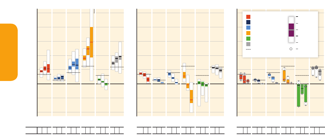
18
SPM
Summary for Policymakers
Infrastructure developments and long-lived products that lock societies into GHG-intensive emissions
pathways may be difficult or very costly to change, reinforcing the importance of early action for ambitious
mitigation (robust evidence, high agreement). This lock-in risk is compounded by the lifetime of the infrastructure, by
the difference in emissions associated with alternatives, and the magnitude of the investment cost. As a result, lock-in
related to infrastructure and spatial planning is the most difficult to reduce. However, materials, products and infrastruc-
ture with long lifetimes and low lifecycle emissions can facilitate a transition to low-emission pathways while also reduc-
ing emissions through lower levels of material use. [5.6.3, 6.3.6.4, 9.4, 10.4, 12.3, 12.4]
There are strong interdependencies in mitigation scenarios between the pace of introducing mitigation
measures in energy supply and energy end-use and developments in the AFOLU sector (high confidence). The
distribution of the mitigation effort across sectors is strongly influenced by the availability and performance of BECCS
and large scale afforestation (Figure SPM.7). This is particularly the case in scenarios reaching CO
2
eq concentrations of
about 450 ppm by 2100. Well-designed systemic and cross-sectoral mitigation strategies are more cost-effective in
cutting emissions than a focus on individual technologies and sectors. At the energy system level these include reduc-
tions in the GHG emission intensity of the energy supply sector, a switch to low-carbon energy carriers (including
low-carbon electricity) and reductions in energy demand in the end-use sectors without compromising development
(Figure SPM.8). [6.3.5, 6.4, 6.8, 7.11, Table TS.2]
Mitigation scenarios reaching around 450 ppm CO
2
eq concentrations by 2100 show large-scale global
changes in the energy supply sector (robust evidence, high agreement). In these selected scenarios, global CO
2
emis-
sions from the energy supply sector are projected to decline over the next decades and are characterized by reductions of
90 % or more below 2010 levels between 2040 and 2070. Emissions in many of these scenarios are projected to decline
to below zero thereafter. [6.3.4, 6.8, 7.1, 7.11]
Figure SPM.7 | Direct emissions of CO
2
by sector and total non-CO
2
GHGs (Kyoto gases) across sectors in baseline (left panel) and mitigation scenarios that reach around 450
(430 – 480) ppm CO
2
eq with CCS (middle panel) and without CCS (right panel). The numbers at the bottom of the graphs refer to the number of scenarios included in the range
which differs across sectors and time due to different sectoral resolution and time horizon of models. Note that many models cannot reach about 450 ppm CO
2
eq concentration by
2100 in the absence of CCS, resulting in a low number of scenarios for the right panel. [Figures 6.34 and 6.35]
CO
2
Transport
CO
2
Buildings
CO
2
Industry
CO
2
Electricity
CO
2
Net AFOLU
Non−CO
2
(All Sectors)
Actual 2010 Level
Individual
Scenarios
Min
75%
Max
Median
25%
Direct Sectoral CO
2
and Non-CO
2
GHG Emissions in Baseline and Mitigation Scenarios with and without CCS
93
93
78
80
80
65
80
80
65
147
147
127
131
131
118
121
121
107
2030
2050
2100
29
29
29
22
22
22
22
22
22
36
36
36
32
32
32
36
36
36
2030
2050
2100
Transport Buildings Industry Electricity Net
AFOLU
Non−CO
2
Transport Buildings Industry Electricity Net
AFOLU
Non−CO
2
Transport Buildings Industry Electricity Net
AFOLU
Non−CO
2
5
5
5
3
3
3
3
3
3
5
5
5
6
6
6
6
6
6
2030
2050
2100
30
20
-20
10
-10
0
40
50
30
20
-20
10
-10
0
40
50
30
20
-20
10
-10
0
40
50
Direct Emissions [GtCO
2
eq/yr]
n=
80 GtCO
2
/yr
450 ppm CO
2
eq with CCSBaselines
450 ppm CO
2
eq without CCS
Figure SPM.8 | Final energy demand reduction relative to baseline (upper row) and low-carbon energy carrier shares in final energy (lower row) in the transport, buildings, and
industry sectors by 2030 and 2050 in scenarios from two different CO
2
eq concentration categories compared to sectoral studies assessed in Chapters 8 – 10. The demand reductions
shown by these scenarios do not compromise development. Low-carbon energy carriers include electricity, hydrogen and liquid biofuels in transport, electricity in buildings and
electricity, heat, hydrogen and bioenergy in industry. The numbers at the bottom of the graphs refer to the number of scenarios included in the ranges which differ across sectors
and time due to different sectoral resolution and time horizon of models. [Figures 6.37 and 6.38]
Min
75%
Max
Median
25%
Final Energy Demand Reduction and Low-Carbon Energy Carrier Shares in Energy End-Use Sectors
N= 161 225 161 225 126 189 126 189 126 189 126 189
2030 2050
Transport
Final Energy Demand Reduction Relative to Baseline [%]
2030 2050
Buildings
Final Energy Demand Reduction Relative to Baseline [%]
2030 2050
100
80
60
40
20
0
100
80
60
40
20
0
100
80
60
40
20
0
Industry
Final Energy Demand Reduction Relative to Baseline [%]
Sectoral Studies (Base)
Sectoral Studies (Policy)
Actual 2010 Level
Baselines
530 – 650 ppm CO
2
eq
430 – 530 ppm CO
2
eq
Sectoral Studies (Partial)
Sectoral Studies (Full)
N=
154 130 182 154 130 182 124 103 110 124 103 110 107 86 95 107 86 95
2030 2050
0
20
40
60
100 100 100
80
Transport
Low-Carbon Energy Carrier Share in Final Energy [%]
2030 2050
0
20
40
60
80
Buildings
Low-Carbon Energy Carrier Share in Final Energy [%]
2030 2050
0
20
40
60
80
Industry
Low-Carbon Energy Carrier Share in Final Energy [%]
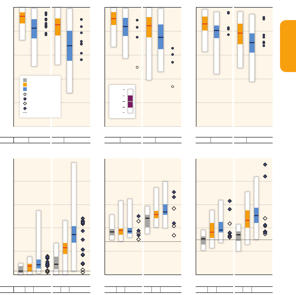
19
SPM
Summary for Policymakers
Infrastructure developments and long-lived products that lock societies into GHG-intensive emissions
pathways may be difficult or very costly to change, reinforcing the importance of early action for ambitious
mitigation (robust evidence, high agreement). This lock-in risk is compounded by the lifetime of the infrastructure, by
the difference in emissions associated with alternatives, and the magnitude of the investment cost. As a result, lock-in
related to infrastructure and spatial planning is the most difficult to reduce. However, materials, products and infrastruc-
ture with long lifetimes and low lifecycle emissions can facilitate a transition to low-emission pathways while also reduc-
ing emissions through lower levels of material use. [5.6.3, 6.3.6.4, 9.4, 10.4, 12.3, 12.4]
There are strong interdependencies in mitigation scenarios between the pace of introducing mitigation
measures in energy supply and energy end-use and developments in the AFOLU sector (high confidence). The
distribution of the mitigation effort across sectors is strongly influenced by the availability and performance of BECCS
and large scale afforestation (Figure SPM.7). This is particularly the case in scenarios reaching CO
2
eq concentrations of
about 450 ppm by 2100. Well-designed systemic and cross-sectoral mitigation strategies are more cost-effective in
cutting emissions than a focus on individual technologies and sectors. At the energy system level these include reduc-
tions in the GHG emission intensity of the energy supply sector, a switch to low-carbon energy carriers (including
low-carbon electricity) and reductions in energy demand in the end-use sectors without compromising development
(Figure SPM.8). [6.3.5, 6.4, 6.8, 7.11, Table TS.2]
Mitigation scenarios reaching around 450 ppm CO
2
eq concentrations by 2100 show large-scale global
changes in the energy supply sector (robust evidence, high agreement). In these selected scenarios, global CO
2
emis-
sions from the energy supply sector are projected to decline over the next decades and are characterized by reductions of
90 % or more below 2010 levels between 2040 and 2070. Emissions in many of these scenarios are projected to decline
to below zero thereafter. [6.3.4, 6.8, 7.1, 7.11]
Figure SPM.7 | Direct emissions of CO
2
by sector and total non-CO
2
GHGs (Kyoto gases) across sectors in baseline (left panel) and mitigation scenarios that reach around 450
(430 – 480) ppm CO
2
eq with CCS (middle panel) and without CCS (right panel). The numbers at the bottom of the graphs refer to the number of scenarios included in the range
which differs across sectors and time due to different sectoral resolution and time horizon of models. Note that many models cannot reach about 450 ppm CO
2
eq concentration by
2100 in the absence of CCS, resulting in a low number of scenarios for the right panel. [Figures 6.34 and 6.35]
CO
2
Transport
CO
2
Buildings
CO
2
Industry
CO
2
Electricity
CO
2
Net AFOLU
Non−CO
2
(All Sectors)
Actual 2010 Level
Individual
Scenarios
Min
75%
Max
Median
25%
Direct Sectoral CO
2
and Non-CO
2
GHG Emissions in Baseline and Mitigation Scenarios with and without CCS
93
93
78
80
80
65
80
80
65
147
147
127
131
131
118
121
121
107
2030
2050
2100
29
29
29
22
22
22
22
22
22
36
36
36
32
32
32
36
36
36
2030
2050
2100
Transport Buildings Industry Electricity Net
AFOLU
Non−CO
2
Transport Buildings Industry Electricity Net
AFOLU
Non−CO
2
Transport Buildings Industry Electricity Net
AFOLU
Non−CO
2
5
5
5
3
3
3
3
3
3
5
5
5
6
6
6
6
6
6
2030
2050
2100
30
20
-20
10
-10
0
40
50
30
20
-20
10
-10
0
40
50
30
20
-20
10
-10
0
40
50
Direct Emissions [GtCO
2
eq/yr]
n=
80 GtCO
2
/yr
450 ppm CO
2
eq with CCSBaselines
450 ppm CO
2
eq without CCS
Figure SPM.8 | Final energy demand reduction relative to baseline (upper row) and low-carbon energy carrier shares in final energy (lower row) in the transport, buildings, and
industry sectors by 2030 and 2050 in scenarios from two different CO
2
eq concentration categories compared to sectoral studies assessed in Chapters 8 – 10. The demand reductions
shown by these scenarios do not compromise development. Low-carbon energy carriers include electricity, hydrogen and liquid biofuels in transport, electricity in buildings and
electricity, heat, hydrogen and bioenergy in industry. The numbers at the bottom of the graphs refer to the number of scenarios included in the ranges which differ across sectors
and time due to different sectoral resolution and time horizon of models. [Figures 6.37 and 6.38]
Min
75%
Max
Median
25%
Final Energy Demand Reduction and Low-Carbon Energy Carrier Shares in Energy End-Use Sectors
N= 161 225 161 225 126 189 126 189 126 189 126 189
2030 2050
Transport
Final Energy Demand Reduction Relative to Baseline [%]
2030 2050
Buildings
Final Energy Demand Reduction Relative to Baseline [%]
2030 2050
100
80
60
40
20
0
100
80
60
40
20
0
100
80
60
40
20
0
Industry
Final Energy Demand Reduction Relative to Baseline [%]
Sectoral Studies (Base)
Sectoral Studies (Policy)
Actual 2010 Level
Baselines
530 – 650 ppm CO
2
eq
430 – 530 ppm CO
2
eq
Sectoral Studies (Partial)
Sectoral Studies (Full)
N=
154 130 182 154 130 182 124 103 110 124 103 110 107 86 95 107 86 95
2030 2050
0
20
40
60
100 100 100
80
Transport
Low-Carbon Energy Carrier Share in Final Energy [%]
2030 2050
0
20
40
60
80
Buildings
Low-Carbon Energy Carrier Share in Final Energy [%]
2030 2050
0
20
40
60
80
Industry
Low-Carbon Energy Carrier Share in Final Energy [%]

20
SPM
Summary for Policymakers
Efficiency enhancements and behavioural changes, in order to reduce energy demand compared to base-
line scenarios without compromising development, are a key mitigation strategy in scenarios reaching
atmospheric CO
2
eq concentrations of about 450 to about 500 ppm by 2100 (robust evidence, high agreement).
Near-term reductions in energy demand are an important element of cost-effective mitigation strategies, provide more
flexibility for reducing carbon intensity in the energy supply sector, hedge against related supply-side risks, avoid lock-in
to carbon-intensive infrastructures, and are associated with important co-benefits. Both integrated and sectoral studies
provide similar estimates for energy demand reductions in the transport, buildings and industry sectors for 2030 and
2050 (Figure SPM.8). [6.3.4, 6.6, 6.8, 7.11, 8.9, 9.8, 10.10]
Behaviour, lifestyle and culture have a considerable influence on energy use and associated emissions, with
high mitigation potential in some sectors, in particular when complementing technological and structural
change
23
(medium evidence, medium agreement). Emissions can be substantially lowered through changes in consump-
tion patterns (e. g., mobility demand and mode, energy use in households, choice of longer-lasting products) and dietary
change and reduction in food wastes. A number of options including monetary and non-monetary incentives as well as
information measures may facilitate behavioural changes. [6.8, 7.9, 8.3.5, 8.9, 9.2, 9.3, 9.10, Box 10.2, 10.4, 11.4, 12.4,
12.6, 12.7, 15.3, 15.5, Table TS.2]
Energy supply
In the baseline scenarios assessed in AR5, direct CO
2
emissions from the energy supply sector are projected
to almost double or even triple by 2050 compared to the level of 14.4 GtCO
2
/ year in 2010, unless energy
intensity improvements can be significantly accelerated beyond the historical development (medium evidence,
medium agreement). In the last decade, the main contributors to emission growth were a growing energy demand and
an increase of the share of coal in the global fuel mix. The availability of fossil fuels alone will not be sufficient to limit
CO
2
eq concentration to levels such as 450 ppm, 550 ppm, or 650 ppm. (Figure SPM.7) [6.3.4, 7.2, 7.3, Figures 6.15, TS.15]
Decarbonizing (i. e. reducing the carbon intensity of) electricity generation is a key component of cost-
effective mitigation strategies in achieving low-stabilization levels (430 – 530 ppm CO
2
eq); in most integrated
modelling scenarios, decarbonization happens more rapidly in electricity generation than in the industry,
buildings, and transport sectors (medium evidence, high agreement) (Figure SPM.7). In the majority of low-stabiliza-
tion scenarios, the share of low-carbon electricity supply (comprising renewable energy (RE), nuclear and CCS) increases
from the current share of approximately 30 % to more than 80 % by 2050, and fossil fuel power generation without CCS
is phased out almost entirely by 2100 (Figure SPM. 7). [6.8, 7.11, Figures 7.14, TS.18]
Since AR4, many RE technologies have demonstrated substantial performance improvements and cost reduc-
tions, and a growing number of RE technologies have achieved a level of maturity to enable deployment at
significant scale (robust evidence, high agreement). Regarding electricity generation alone, RE accounted for just over
half of the new electricity-generating capacity added globally in 2012, led by growth in wind, hydro and solar power.
However, many RE technologies still need direct and / or indirect support, if their market shares are to be significantly
increased; RE technology policies have been successful in driving recent growth of RE. Challenges for integrating RE into
energy systems and the associated costs vary by RE technology, regional circumstances, and the characteristics of the
existing background energy system (medium evidence, medium agreement). [7.5.3, 7.6.1, 7.8.2, 7.12, Table 7.1]
Nuclear energy is a mature low-GHG emission source of baseload power, but its share of global electricity
generation has been declining (since 1993). Nuclear energy could make an increasing contribution to low-
carbon energy supply, but a variety of barriers and risks exist (robust evidence, high agreement). Those include:
23
Structural changes refer to systems transformations whereby some components are either replaced or potentially substituted by other compo-
nents (see WGIII AR5 Glossary).
SPM.4.2.2

21
SPM
Summary for Policymakers
operational risks, and the associated concerns, uranium mining risks, financial and regulatory risks, unresolved waste
management issues, nuclear weapon proliferation concerns, and adverse public opinion (robust evidence, high agree-
ment). New fuel cycles and reactor technologies addressing some of these issues are being investigated and progress in
research and development has been made concerning safety and waste disposal. [7.5.4, 7.8, 7.9, 7.12, Figure TS.19]
GHG emissions from energy supply can be reduced significantly by replacing current world average coal-fired
power plants with modern, highly efficient natural gas combined-cycle power plants or combined heat and
power plants, provided that natural gas is available and the fugitive emissions associated with extraction
and supply are low or mitigated (robust evidence, high agreement). In mitigation scenarios reaching about 450 ppm
CO
2
eq concentrations by 2100, natural gas power generation without CCS acts as a bridge technology, with deployment
increasing before peaking and falling to below current levels by 2050 and declining further in the second half of the
century (robust evidence, high agreement). [7.5.1, 7.8, 7.9, 7.11, 7.12]
Carbon dioxide capture and storage (CCS) technologies could reduce the lifecycle GHG emissions of fos-
sil fuel power plants (medium evidence, medium agreement). While all components of integrated CCS systems exist
and are in use today by the fossil fuel extraction and refining industry, CCS has not yet been applied at scale to a large,
operational commercial fossil fuel power plant. CCS power plants could be seen in the market if this is incentivized by
regulation and /or if they become competitive with their unabated counterparts, for instance, if the additional investment
and operational costs, caused in part by efficiency reductions, are compensated by sufficiently high carbon prices (or
direct financial support). For the large-scale future deployment of CCS, well-defined regulations concerning short- and
long-term responsibilities for storage are needed as well as economic incentives. Barriers to large-scale deployment of
CCS technologies include concerns about the operational safety and long-term integrity of CO
2
storage as well as trans-
port risks. There is, however, a growing body of literature on how to ensure the integrity of CO
2
wells, on the potential
consequences of a pressure build-up within a geologic formation caused by CO
2
storage (such as induced seismicity),
and on the potential human health and environmental impacts from CO
2
that migrates out of the primary injection zone
(limited evidence, medium agreement). [7.5.5., 7.8, 7.9, 7.11, 7.12, 11.13]
Combining bioenergy with CCS (BECCS) offers the prospect of energy supply with large-scale net negative
emissions which plays an important role in many low-stabilization scenarios, while it entails challenges and
risks (limited evidence, medium agreement). These challenges and risks include those associated with the upstream
large-scale provision of the biomass that is used in the CCS facility as well as those associated with the CCS technology
itself. [7.5.5, 7.9, 11.13]
Energy end-use sectors
Transport
The transport sector accounted for 27 % of final energy use and 6.7 GtCO
2
direct emissions in 2010, with
baseline CO
2
emissions projected to approximately double by 2050 (medium evidence, medium agreement). This
growth in CO
2
emissions from increasing global passenger and freight activity could partly offset future mitigation mea-
sures that include fuel carbon and energy intensity improvements, infrastructure development, behavioural change and
comprehensive policy implementation (high confidence). Overall, reductions in total transport CO
2
emissions of 15 – 40 %
compared to baseline growth could be achieved in 2050 (medium evidence, medium agreement). (Figure SPM.7) [6.8,
8.1, 8.2, 8.9, 8.10]
Technical and behavioural mitigation measures for all transport modes, plus new infrastructure and urban
redevelopment investments, could reduce final energy demand in 2050 by around 40 % below the baseline,
with the mitigation potential assessed to be higher than reported in the AR4 (robust evidence, medium agree-
ment). Projected energy efficiency and vehicle performance improvements range from 30 – 50 % in 2030 relative to 2010
depending on transport mode and vehicle type (medium evidence, medium agreement). Integrated urban planning,
SPM.4.2.3

22
SPM
Summary for Policymakers
transit-oriented development, more compact urban form that supports cycling and walking, can all lead to modal shifts
as can, in the longer term, urban redevelopment and investments in new infrastructure such as high-speed rail systems
that reduce short-haul air travel demand (medium evidence, medium agreement). Such mitigation measures are chal-
lenging, have uncertain outcomes, and could reduce transport GHG emissions by 20 – 50 % in 2050 compared to baseline
(limited evidence, low agreement). (Figure SPM.8 upper panel) [8.2, 8.3, 8.4, 8.5, 8.6, 8.7, 8.8, 8.9, 12.4, 12.5]
Strategies to reduce the carbon intensities of fuel and the rate of reducing carbon intensity are constrained by
challenges associated with energy storage and the relatively low energy density of low-carbon transport fuels
(medium confidence). Integrated and sectoral studies broadly agree that opportunities for switching to low-carbon fuels
exist in the near term and will grow over time. Methane-based fuels are already increasing their share for road vehicles
and waterborne craft. Electricity produced from low-carbon sources has near-term potential for electric rail and short- to
medium-term potential as electric buses, light-duty and 2-wheel road vehicles are deployed. Hydrogen fuels from low-car-
bon sources constitute longer-term options. Commercially available liquid and gaseous biofuels already provide co-benefits
together with mitigation options that can be increased by technology advances. Reducing transport emissions of particulate
matter (including black carbon), tropospheric ozone and aerosol precursors (including NO
x
) can have human health and
mitigation co-benefits in the short term (medium evidence, medium agreement). [8.2, 8.3, 11.13, Figure TS.20, right panel]
The cost-effectiveness of different carbon reduction measures in the transport sector varies significantly with
vehicle type and transport mode (high confidence). The levelized costs of conserved carbon can be very low or nega-
tive for many short-term behavioural measures and efficiency improvements for light- and heavy-duty road vehicles and
waterborne craft. In 2030, for some electric vehicles, aircraft and possibly high-speed rail, levelized costs could be more
than USD100 / tCO
2
avoided (limited evidence, medium agreement). [8.6, 8.8, 8.9, Figures TS.21, TS.22]
Regional differences influence the choice of transport mitigation options (high confidence). Institutional, legal,
financial and cultural barriers constrain low-carbon technology uptake and behavioural change. Established infrastructure
may limit the options for modal shift and lead to a greater reliance on advanced vehicle technologies; a slowing of growth
in light-duty vehicle demand is already evident in some OECD countries. For all economies, especially those with high rates
of urban growth, investment in public transport systems and low-carbon infrastructure can avoid lock-in to carbon-intensive
modes. Prioritizing infrastructure for pedestrians and integrating non-motorized and transit services can create economic
and social co-benefits in all regions (medium evidence, medium agreement). [8.4, 8.8, 8.9, 14.3, Table 8.3]
Mitigation strategies, when associated with non-climate policies at all government levels, can help decouple
transport GHG emissions from economic growth in all regions (medium confidence). These strategies can help
reduce travel demand, incentivise freight businesses to reduce the carbon intensity of their logistical systems and induce
modal shifts, as well as provide co-benefits including improved access and mobility, better health and safety, greater
energy security, and cost and time savings (medium evidence, high agreement). [8.7, 8.10]
Buildings
In 2010, the buildings sector
24
accounted for around 32 % final energy use and 8.8 GtCO
2
emissions, including
direct and indirect emissions, with energy demand projected to approximately double and CO
2
emissions to
increase by 50 – 150 % by mid-century in baseline scenarios (medium evidence, medium agreement). This energy
demand growth results from improvements in wealth, lifestyle change, access to modern energy services and adequate
housing, and urbanisation. There are significant lock-in risks associated with the long lifespans of buildings and related
infrastructure, and these are especially important in regions with high construction rates (robust evidence, high agree-
ment). (Figure SPM.7) [9.4]
24
The buildings sector covers the residential, commercial, public and services sectors; emissions from construction are accounted for in the industry sec-
tor.

23
SPM
Summary for Policymakers
Recent advances in technologies, know-how and policies provide opportunities to stabilize or reduce global
buildings sector energy use by mid-century (robust evidence, high agreement). For new buildings, the adoption of
very low energy building codes is important and has progressed substantially since AR4. Retrofits form a key part of
the mitigation strategy in countries with established building stocks, and reductions of heating / cooling energy use by
50 – 90 % in individual buildings have been achieved. Recent large improvements in performance and costs make very
low energy construction and retrofits economically attractive, sometimes even at net negative costs. [9.3]
Lifestyle, culture and behaviour significantly influence energy consumption in buildings (limited evidence, high
agreement). A three- to five-fold difference in energy use has been shown for provision of similar building-related energy
service levels in buildings. For developed countries, scenarios indicate that lifestyle and behavioural changes could reduce
energy demand by up to 20 % in the short term and by up to 50 % of present levels by mid-century. In developing coun-
tries, integrating elements of traditional lifestyles into building practices and architecture could facilitate the provision of
high levels of energy services with much lower energy inputs than baseline. [9.3]
Most mitigation options for buildings have considerable and diverse co-benefits in addition to energy cost
savings (robust evidence, high agreement). These include improvements in energy security, health (such as from cleaner
wood-burning cookstoves), environmental outcomes, workplace productivity, fuel poverty reductions and net employ-
ment gains. Studies which have monetized co-benefits often find that these exceed energy cost savings and possibly
climate benefits (medium evidence, medium agreement). [9.6, 9.7, 3.6.3]
Strong barriers, such as split incentives (e. g., tenants and builders), fragmented markets and inadequate
access to information and financing, hinder the market-based uptake of cost-effective opportunities. Barriers
can be overcome by policy interventions addressing all stages of the building and appliance lifecycles (robust evidence,
high agreement). [9.8, 9.10, 16, Box 3.10]
The development of portfolios of energy efficiency policies and their implementation has advanced consider-
ably since AR4. Building codes and appliance standards, if well designed and implemented, have been among
the most environmentally and cost-effective instruments for emission reductions (robust evidence, high agree-
ment). In some developed countries they have contributed to a stabilization of, or reduction in, total energy demand for
buildings. Substantially strengthening these codes, adopting them in further jurisdictions, and extending them to more
building and appliance types, will be a key factor in reaching ambitious climate goals. [9.10, 2.6.5.3]
Industry
In 2010, the industry sector accounted for around 28 % of final energy use, and 13 GtCO
2
emissions, including
direct and indirect emissions as well as process emissions, with emissions projected to increase by 50 – 150 %
by 2050 in the baseline scenarios assessed in AR5, unless energy efficiency improvements are accelerated
significantly (medium evidence, medium agreement). Emissions from industry accounted for just over 30 % of global
GHG emissions in 2010 and are currently greater than emissions from either the buildings or transport end-use sectors.
(Figures SPM.2, SPM.7) [10.3]
The energy intensity of the industry sector could be directly reduced by about 25 % compared to the current
level through the wide-scale upgrading, replacement and deployment of best available technologies, par-
ticularly in countries where these are not in use and in non-energy intensive industries (high agreement, robust
evidence). Additional energy intensity reductions of about 20 % may potentially be realized through innovation (limited
evidence, medium agreement). Barriers to implementing energy efficiency relate largely to initial investment costs and
lack of information. Information programmes are a prevalent approach for promoting energy efficiency, followed by
economic instruments, regulatory approaches and voluntary actions. [10.7, 10.9, 10.11]

24
SPM
Summary for Policymakers
Improvements in GHG emission efficiency and in the efficiency of material use, recycling and re-use of mate-
rials and products, and overall reductions in product demand (e. g., through a more intensive use of products)
and service demand could, in addition to energy efficiency, help reduce GHG emissions below the baseline
level in the industry sector (medium evidence, high agreement). Many emission-reducing options are cost-effective,
profitable and associated with multiple co-benefits (better environmental compliance, health benefits etc.). In the long
term, a shift to low-carbon electricity, new industrial processes, radical product innovations (e. g., alternatives to cement),
or CCS (e. g., to mitigate process emissions) could contribute to significant GHG emission reductions. Lack of policy and
experiences in material and product service efficiency are major barriers. [10.4, 10.7, 10.8, 10.11]
CO
2
emissions dominate GHG emissions from industry, but there are also substantial mitigation opportuni-
ties for non-CO
2
gases (robust evidence, high agreement). CH
4
, N
2
O and fluorinated gases from industry accounted for
emissions of 0.9 GtCO
2
eq in 2010. Key mitigation opportunities include, e. g., the reduction of hydrofluorocarbon emissions
by process optimization and refrigerant recovery, recycling and substitution, although there are barriers. [Tables 10.2, 10.7]
Systemic approaches and collaborative activities across companies and sectors can reduce energy and
material consumption and thus GHG emissions (robust evidence, high agreement). The application of cross-cutting
technologies (e. g., efficient motors) and measures (e. g., reducing air or steam leaks) in both large energy intensive indus-
tries and small and medium enterprises can improve process performance and plant efficiency cost-effectively. Coopera-
tion across companies (e. g., in industrial parks) and sectors could include the sharing of infrastructure, information, and
waste heat utilization. [10.4, 10.5]
Important options for mitigation in waste management are waste reduction, followed by re-use, recycling
and energy recovery (robust evidence, high agreement). Waste and wastewater accounted for 1.5 GtCO
2
eq in 2010.
As the share of recycled or reused material is still low (e. g., globally, around 20 % of municipal solid waste is recycled),
waste treatment technologies and recovering energy to reduce demand for fossil fuels can result in significant direct
emission reductions from waste disposal. [10.4, 10.14]
Agriculture, Forestry and Other Land Use (AFOLU)
The AFOLU sector accounts for about a quarter (~10 – 12 GtCO
2
eq / yr) of net anthropogenic GHG emissions
mainly from deforestation, agricultural emissions from soil and nutrient management and livestock (medium
evidence, high agreement). Most recent estimates indicate a decline in AFOLU CO
2
fluxes, largely due to decreasing
deforestation rates and increased afforestation. However, the uncertainty in historical net AFOLU emissions is larger than
for other sectors, and additional uncertainties in projected baseline net AFOLU emissions exist. Nonetheless, in the future,
net annual baseline CO
2
emissions from AFOLU are projected to decline, with net emissions potentially less than half the
2010 level by 2050 and the possibility of the AFOLU sectors becoming a net CO
2
sink before the end of century (medium
evidence, high agreement). (Figure SPM. 7) [6.3.1.4, 11.2, Figure 6.5]
AFOLU plays a central role for food security and sustainable development. The most cost-effective mitiga-
tion options in forestry are afforestation, sustainable forest management and reducing deforestation, with
large differences in their relative importance across regions. In agriculture, the most cost-effective mitiga-
tion options are cropland management, grazing land management, and restoration of organic soils (medium
evidence, high agreement). The economic mitigation potential of supply-side measures is estimated to be 7.2 to 11
GtCO
2
eq / year
25
in 2030 for mitigation efforts consistent with carbon prices
26
up to 100 USD / tCO
2
eq, about a third of
which can be achieved at a < 20 USD / tCO
2
eq (medium evidence, medium agreement). There are potential barriers to
25
Full range of all studies: 0.49 – 11 GtCO
2
eq / year
26
In many models that are used to assess the economic costs of mitigation, carbon price is used as a proxy to represent the level of effort in mitiga-
tion policies (see WGIII AR5 Glossary).
SPM.4.2.4

25
SPM
Summary for Policymakers
implementation of available mitigation options [11.7, 11.8]. Demand-side measures, such as changes in diet and reduc-
tions of losses in the food supply chain, have a significant, but uncertain, potential to reduce GHG emissions from food
production (medium evidence, medium agreement). Estimates vary from roughly 0.76 – 8.6 GtCO
2
eq / yr by 2050 (limited
evidence, medium agreement). [11.4, 11.6, Figure 11.14]
Policies governing agricultural practices and forest conservation and management are more effective when
involving both mitigation and adaptation. Some mitigation options in the AFOLU sector (such as soil and forest
carbon stocks) may be vulnerable to climate change (medium evidence, high agreement). When implemented sustain-
ably, activities to reduce emissions from deforestation and forest degradation (REDD+
27
is an example designed to be
sustainable) are cost-effective policy options for mitigating climate change, with potential economic, social and other
environmental and adaptation co-benefits (e. g., conservation of biodiversity and water resources, and reducing soil ero-
sion) (limited evidence, medium agreement). [11.3.2, 11.10]
Bioenergy can play a critical role for mitigation, but there are issues to consider, such as the sustainability of
practices and the efficiency of bioenergy systems (robust evidence, medium agreement) [11.4.4, Box 11.5, 11.13.6,
11.13.7]. Barriers to large-scale deployment of bioenergy include concerns about GHG emissions from land, food security,
water resources, biodiversity conservation and livelihoods. The scientific debate about the overall climate impact related
to land-use competition effects of specific bioenergy pathways remains unresolved (robust evidence, high agreement).
[11.4.4, 11.13] Bioenergy technologies are diverse and span a wide range of options and technology pathways. Evidence
suggests that options with low lifecycle emissions (e. g., sugar cane, Miscanthus, fast growing tree species, and sustain-
able use of biomass residues), some already available, can reduce GHG emissions; outcomes are site-specific and rely
on efficient integrated ‘biomass-to-bioenergy systems’, and sustainable land-use management and governance. In some
regions, specific bioenergy options, such as improved cookstoves, and small-scale biogas and biopower production, could
reduce GHG emissions and improve livelihoods and health in the context of sustainable development (medium evidence,
medium agreement). [11.13]
Human settlements, infrastructure and spatial planning
Urbanization is a global trend and is associated with increases in income, and higher urban incomes are cor-
related with higher consumption of energy and GHG emissions (medium evidence, high agreement). As of 2011,
more than 52 % of the global population lives in urban areas. In 2006, urban areas accounted for 67 – 76 % of energy use
and 71 – 76 % of energy-related CO
2
emissions. By 2050, the urban population is expected to increase to 5.6 – 7.1 billion,
or 64 – 69 % of world population. Cities in non-Annex I countries generally have higher levels of energy use compared to
the national average, whereas cities in Annex I countries generally have lower energy use per capita than national aver-
ages (medium evidence, medium agreement). [12.2, 12.3]
The next two decades present a window of opportunity for mitigation in urban areas, as a large portion of
the world’s urban areas will be developed during this period (limited evidence, high agreement). Accounting for
trends in declining population densities, and continued economic and population growth, urban land cover is projected
to expand by 56 – 310 % between 2000 and 2030. [12.2, 12.3, 12.4, 12.8]
Mitigation options in urban areas vary by urbanization trajectories and are expected to be most effective
when policy instruments are bundled (robust evidence, high agreement). Infrastructure and urban form are strongly
interlinked, and lock-in patterns of land use, transport choice, housing, and behaviour. Effective mitigation strategies
involve packages of mutually reinforcing policies, including co-locating high residential with high employment densities,
27
See WGIII AR5 Glossary.
SPM.4.2.5

26
SPM
Summary for Policymakers
achieving high diversity and integration of land uses, increasing accessibility and investing in public transport and other
demand management measures. [8.4, 12.3, 12.4, 12.5, 12.6]
The largest mitigation opportunities with respect to human settlements are in rapidly urbanizing areas where
urban form and infrastructure are not locked in, but where there are often limited governance, technical,
financial, and institutional capacities (robust evidence, high agreement). The bulk of urban growth is expected in
small- to medium-size cities in developing countries. The feasibility of spatial planning instruments for climate change
mitigation is highly dependent on a city’s financial and governance capability. [12.6, 12.7]
Thousands of cities are undertaking climate action plans, but their aggregate impact on urban emissions
is uncertain (robust evidence, high agreement). There has been little systematic assessment on their implementation,
the extent to which emission reduction targets are being achieved, or emissions reduced. Current climate action plans
focus largely on energy efficiency. Fewer climate action plans consider land-use planning strategies and cross-sectoral
measures to reduce sprawl and promote transit-oriented development
28
. [12.6, 12.7, 12.9]
Successful implementation of urban-scale climate change mitigation strategies can provide co-benefits
(robust evidence, high agreement). Urban areas throughout the world continue to struggle with challenges, including
ensuring access to energy, limiting air and water pollution, and maintaining employment opportunities and competitive-
ness. Action on urban-scale mitigation often depends on the ability to relate climate change mitigation efforts to local
co-benefits (robust evidence, high agreement). [12.5, 12.6, 12.7, 12.8]
Mitigation policies and institutions
Sectoral and national policies
Substantial reductions in emissions would require large changes in investment patterns. Mitigation scenarios
in which policies stabilize atmospheric concentrations (without overshoot) in the range from 430 to 530 ppm CO
2
eq by
2100 lead to substantial shifts in annual investment flows during the period 2010 – 2029 compared to baseline scenarios
(Figure SPM.9). Over the next two decades (2010 to 2029), annual investment in conventional fossil fuel technologies
associated with the electricity supply sector is projected to decline by about 30 (2 – 166) billion USD (median: − 20 %
compared to 2010) while annual investment in low-carbon electricity supply (i. e., renewables, nuclear and electric-
ity generation with CCS) is projected to rise by about 147 (31 – 360) billion USD (median: + 100 % compared to 2010)
(limited evidence, medium agreement). For comparison, global total annual investment in the energy system is presently
about 1200 billion USD. In addition, annual incremental energy efficiency investments in transport, buildings and industry
is projected to increase by about 336 (1 – 641) billion USD (limited evidence, medium agreement), frequently involving
modernization of existing equipment. [13.11, 16.2.2]
There is no widely agreed definition of what constitutes climate finance, but estimates of the financial flows
associated with climate change mitigation and adaptation are available. Published assessments of all current
annual financial flows whose expected effect is to reduce net GHG emissions and / or to enhance resilience to climate
change and climate variability show 343 to 385 billion USD per year globally (medium confidence) [Box TS.14]. Most of
this goes to mitigation. Out of this, total public climate finance that flowed to developing countries is estimated to be
between 35 and 49 billion USD / yr in 2011 and 2012 (medium confidence). Estimates of international private climate
28
See WGIII AR5 Glossary.
SPM.5
SPM.5.1
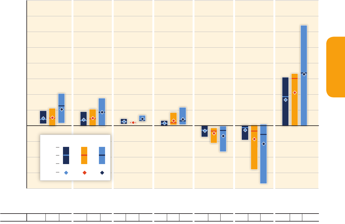
27
SPM
Summary for Policymakers
finance flowing to developing countries range from 10 to 72 billion USD / yr including foreign direct investment as equity
and loans in the range of 10 to 37 billion USD / yr over the period of 2008 – 2011 (medium confidence). [16.2.2]
There has been a considerable increase in national and sub-national mitigation plans and strategies since AR4.
In 2012, 67 % of global GHG emissions were subject to national legislation or strategies versus 45 % in 2007. However,
there has not yet been a substantial deviation in global emissions from the past trend [Figure 1.3c]. These plans and
strategies are in their early stages of development and implementation in many countries, making it difficult to assess their
aggregate impact on future global emissions (medium evidence, high agreement). [14.3.4, 14.3.5, 15.1, 15.2]
Since AR4, there has been an increased focus on policies designed to integrate multiple objectives, increase
co-benefits and reduce adverse side-effects (high confidence). Governments often explicitly reference co-benefits in
climate and sectoral plans and strategies. The scientific literature has sought to assess the size of co-benefits (see Sec-
tion SPM.4.1) and the greater political feasibility and durability of policies that have large co-benefits and small adverse
Figure SPM.9 | Change in annual investment flows from the average baseline level over the next two decades (2010 – 2029) for mitigation scenarios that stabilize concentrations
within the range of approximately 430 – 530 ppm CO
2
eq by 2100. Investment changes are based on a limited number of model studies and model comparisons. Total electricity gen-
eration (leftmost column) is the sum of renewables, nuclear, power plants with CCS and fossil fuel power plants without CCS. The vertical bars indicate the range between minimum
and maximum estimate; the horizontal bar indicates the median. Proximity to this median value does not imply higher likelihood because of the different degree of aggregation of
model results, the low number of studies available and different assumptions in the different studies considered. The numbers in the bottom row show the total number of stud-
ies in the literature used for the assessment. This underscores that investment needs are still an evolving area of research that relatively few studies have examined. [Figure 16.3]
-400
-300
-200
-100
0
100
200
300
400
500
600
700
800
Power Plants
with CCS
Renewables Energy Efficiency
Across Sectors
Extraction of
Fossil Fuels
Fossil Fuel
Power Plants
without CCS
NuclearTotal Electricity
Generation
# of Studies: 434444444 3545
545455 44
Changes in Annual Investment Flows 2010 – 2029 [Billion USD
2010
/yr]
Max
Median
Mean
Min
non-OECD
WorldOECD

28
SPM
Summary for Policymakers
side-effects. [4.8, 5.7, 6.6, 13.2, 15.2] Despite the growing attention in policymaking and the scientific literature since AR4,
the analytical and empirical underpinnings for understanding many of the interactive effects are under-developed [1.2,
3.6.3, 4.2, 4.8, 5.7, 6.6].
Sector-specific policies have been more widely used than economy-wide policies (medium evidence, high agree-
ment). Although most economic theory suggests that economy-wide policies for the singular objective of mitigation
would be more cost-effective than sector-specific policies, since AR4 a growing number of studies has demonstrated that
administrative and political barriers may make economy-wide policies harder to design and implement than sector-spe-
cific policies. The latter may be better suited to address barriers or market failures specific to certain sectors, and may be
bundled in packages of complementary policies. [6.3.6.5, 8.10, 9.10, 10.10, 15.2, 15.5, 15.8, 15.9]
Regulatory approaches and information measures are widely used, and are often environmentally effec-
tive (medium evidence, medium agreement). Examples of regulatory approaches include energy efficiency standards;
examples of information programmes include labelling programmes that can help consumers make better-informed deci-
sions. While such approaches have often been found to have a net social benefit, the scientific literature is divided on the
extent to which such policies can be implemented with negative private costs to firms and individuals. [Box 3.10, 15.5.5,
15.5.6] There is general agreement that rebound effects exist, whereby higher efficiency can lead to lower energy prices
and greater consumption, but there is low agreement in the literature on the magnitude [3.9.5, 5.7.2, 14.4.2, 15.5.4].
Since AR4, cap and trade systems for GHGs have been established in a number of countries and regions. Their
short-run environmental effect has been limited as a result of loose caps or caps that have not proved to
be constraining (limited evidence, medium agreement). This was related to factors such as the financial and economic
crisis that reduced energy demand, new energy sources, interactions with other policies, and regulatory uncertainty. In
principle, a cap and trade system can achieve mitigation in a cost-effective way; its implementation depends on national
circumstances. Though earlier programmes relied almost exclusively on grandfathering (free allocation of permits), auc-
tioning permits is increasingly applied. If allowances are auctioned, revenues can be used to address other investments
with a high social return, and / or reduce the tax and debt burden. [14.4.2, 15.5.3]
In some countries, tax-based policies specifically aimed at reducing GHG emissions—alongside technology
and other policies—have helped to weaken the link between GHG emissions and GDP (high confidence). In
a large group of countries, fuel taxes (although not necessarily designed for the purpose of mitigation) have effects
that are akin to sectoral carbon taxes [Table 15.2]. The demand reduction in transport fuel associated with a 1 % price
increase is 0.6 % to 0.8 % in the long run, although the short-run response is much smaller [15.5.2]. In some countries
revenues are used to reduce other taxes and / or to provide transfers to low-income groups. This illustrates the general
principle that mitigation policies that raise government revenue generally have lower social costs than approaches which
do not. While it has previously been assumed that fuel taxes in the transport sector are regressive, there have been a
number of other studies since AR4 that have shown them to be progressive, particularly in developing countries (medium
evidence, medium agreement). [3.6.3, 14.4.2, 15.5.2]
The reduction of subsidies for GHG-related activities in various sectors can achieve emission reductions,
depending on the social and economic context (high confidence). While subsidies can affect emissions in many sec-
tors, most of the recent literature has focused on subsidies for fossil fuels. Since AR4 a small but growing literature based
on economy-wide models has projected that complete removal of subsidies for fossil fuels in all countries could result in
reductions in global aggregate emissions by mid-century (medium evidence, medium agreement) [7.12, 13.13, 14.3.2,
15.5.2]. Studies vary in methodology, the type and definition of subsidies and the time frame for phase out considered. In
particular, the studies assess the impacts of complete removal of all fossil fuel subsidies without seeking to assess which
subsidies are wasteful and inefficient, keeping in mind national circumstances. Although political economy barriers are
substantial, some countries have reformed their tax and budget systems to reduce fuel subsidies. To help reduce possible
adverse effects on lower-income groups who often spend a large fraction of their income on energy services, many gov-
ernments have utilized lump-sum cash transfers or other mechanisms targeted on the poor. [15.5.2]

29
SPM
Summary for Policymakers
Interactions between or among mitigation policies may be synergistic or may have no additive effect on
reducing emissions (medium evidence, high agreement). For instance, a carbon tax can have an additive environmental
effect to policies such as subsidies for the supply of RE. By contrast, if a cap and trade system has a binding cap (suffi-
ciently stringent to affect emission-related decisions), then other policies such as RE subsidies have no further impact on
reducing emissions within the time period that the cap applies (although they may affect costs and possibly the viability
of more stringent future targets) (medium evidence, high agreement). In either case, additional policies may be needed to
address market failures relating to innovation and technology diffusion. [15.7]
Some mitigation policies raise the prices for some energy services and could hamper the ability of societ-
ies to expand access to modern energy services to underserved populations (low confidence). These potential
adverse side-effects can be avoided with the adoption of complementary policies (medium confidence). Most
notably, about 1.3 billion people worldwide do not have access to electricity and about 3 billion are dependent on tradi-
tional solid fuels for cooking and heating with severe adverse effects on health, ecosystems and development. Provid-
ing access to modern energy services is an important sustainable development objective. The costs of achieving nearly
universal access to electricity and clean fuels for cooking and heating are projected to be between 72 and 95 billion USD
per year until 2030 with minimal effects on GHG emissions (limited evidence, medium agreement). A transition away
from the use of traditional biomass
29
and the more efficient combustion of solid fuels reduce air pollutant emissions, such
as sulfur dioxide (SO
2
), nitrogen oxides (NO
x
), carbon monoxide (CO), and black carbon (BC), and thus yield large health
benefits (high confidence). [4.3, 6.6, 7.9, 9.3, 9.7, 11.13.6, 16.8]
Technology policy complements other mitigation policies (high confidence). Technology policy includes techno logy-
push (e. g., publicly funded R&D) and demand-pull (e. g., governmental procurement programmes). Such policies address
market failures related to innovation and technology diffusion. [3.11, 15.6] Technology support policies have promoted
substantial innovation and diffusion of new technologies, but the cost-effectiveness of such policies is often difficult to
assess [2.6.5, 7.12, 9.10]. Nevertheless, program evaluation data can provide empirical evidence on the relative effective-
ness of different policies and can assist with policy design [15.6.5].
In many countries, the private sector plays central roles in the processes that lead to emissions as well as to
mitigation. Within appropriate enabling environments, the private sector, along with the public sector, can
play an important role in financing mitigation (medium evidence, high agreement). The share of total mitigation
finance from the private sector, acknowledging data limitations, is estimated to be on average between two-thirds and
three-fourths on the global level (2010 – 2012) (limited evidence, medium agreement). In many countries, public finance
interventions by governments and national and international development banks encourage climate investments by the
private sector [16.2.1] and provide finance where private sector investment is limited. The quality of a country’s enabling
environment includes the effectiveness of its institutions, regulations and guidelines regarding the private sector, security
of property rights, credibility of policies and other factors that have a substantial impact on whether private firms invest
in new technologies and infrastructures [16.3]. Dedicated policy instruments, for example, credit insurance, power
purchase agreements and feed-in tariffs, concessional finance or rebates, provide an incentive for investment by lowering
risks for private actors [16.4].
29
See WGIII AR5 Glossary.

30
SPM
Summary for Policymakers
International cooperation
The United Nations Framework Convention on Climate Change (UNFCCC) is the main multilateral forum
focused on addressing climate change, with nearly universal participation. Other institutions organized at differ-
ent levels of governance have resulted in diversifying international climate change cooperation. [13.3.1, 13.4.1.4, 13.5]
Existing and proposed international climate change cooperation arrangements vary in their focus and degree
of centralization and coordination. They span: multilateral agreements, harmonized national policies and decentral-
ized but coordinated national policies, as well as regional and regionally-coordinated policies. [Figure TS.38, 13.4.1,
13.13.2, 14.4]
The Kyoto Protocol offers lessons towards achieving the ultimate objective of the UNFCCC, particularly with
respect to participation, implementation, flexibility mechanisms, and environmental effectiveness (medium
evidence, low agreement). [5.3.3, 13.3.4, 13.7.2, 13.13.1.1, 13.13.1.2, 14.3.7.1, Table TS.9]
UNFCCC activities since 2007 have led to an increasing number of institutions and other arrangements for
international climate change cooperation. [13.5.1.1, 13.13.1.3, 16.2.1]
Policy linkages among regional, national, and sub-national climate policies offer potential climate change
mitigation and adaptation benefits (medium evidence, medium agreement). Linkages can be established between
national policies, various instruments, and through regional cooperation. [13.3.1, 13.5.3, 13.6, 13.7, 13.13.2.3, 14.4,
Figure 13.4]
Various regional initiatives between the national and global scales are either being developed or imple-
mented, but their impact on global mitigation has been limited to date (medium confidence). Many climate
policies can be more effective if implemented across geographical regions. [13.13, 13.6, 14.4, 14.5]
SPM.5.2
