1029

This chapter should be cited as:

Collins, M., R. Knutti, J. Arblaster, J.-L. Dufresne, T. Fichefet, P. Friedlingstein, X. Gao, W.J. Gutowski, T. Johns, G.

Krinner, M. Shongwe, C. Tebaldi, A.J. Weaver and M. Wehner, 2013: Long-term Climate Change: Projections, Com-

mitments and Irreversibility. In: Climate Change 2013: The Physical Science Basis. Contribution of Working Group

I to the Fifth Assessment Report of the Intergovernmental Panel on Climate Change [Stocker, T.F., D. Qin, G.-K.

Plattner, M. Tignor, S.K. Allen, J. Boschung, A. Nauels, Y. Xia, V. Bex and P.M. Midgley (eds.)]. Cambridge University

Press, Cambridge, United Kingdom and New York, NY, USA.

Coordinating Lead Authors:

Matthew Collins (UK), Reto Knutti (Switzerland)

Lead Authors:

Julie Arblaster (Australia), Jean-Louis Dufresne (France), Thierry Fichefet (Belgium), Pierre

Friedlingstein (UK/Belgium), Xuejie Gao (China), William J. Gutowski Jr. (USA), Tim Johns (UK),

Gerhard Krinner (France/Germany), Mxolisi Shongwe (South Africa), Claudia Tebaldi (USA),

Andrew J. Weaver (Canada), Michael Wehner (USA)

Contributing Authors:

Myles R. Allen (UK), Tim Andrews (UK), Urs Beyerle (Switzerland), Cecilia M. Bitz (USA),

Sandrine Bony (France), Ben B.B. Booth (UK), Harold E. Brooks (USA), Victor Brovkin (Germany),

Oliver Browne (UK), Claire Brutel-Vuilmet (France), Mark Cane (USA), Robin Chadwick (UK),

Ed Cook (USA), Kerry H. Cook (USA), Michael Eby (Canada), John Fasullo (USA), Erich M.

Fischer (Switzerland), Chris E. Forest (USA), Piers Forster (UK), Peter Good (UK), Hugues Goosse

(Belgium), Jonathan M. Gregory (UK), Gabriele C. Hegerl (UK/Germany), Paul J. Hezel (Belgium/

USA), Kevin I. Hodges (UK), Marika M. Holland (USA), Markus Huber (Switzerland), Philippe

Huybrechts (Belgium), Manoj Joshi (UK), Viatcheslav Kharin (Canada), Yochanan Kushnir (USA),

David M. Lawrence (USA), Robert W. Lee (UK), Spencer Liddicoat (UK), Christopher Lucas

(Australia), Wolfgang Lucht (Germany), Jochem Marotzke (Germany), François Massonnet

(Belgium), H. Damon Matthews (Canada), Malte Meinshausen (Germany), Colin Morice

(UK), Alexander Otto (UK/Germany), Christina M. Patricola (USA), Gwenaëlle Philippon-

Berthier (France), Prabhat (USA), Stefan Rahmstorf (Germany), William J. Riley (USA), Joeri

Rogelj (Switzerland/Belgium), Oleg Saenko (Canada), Richard Seager (USA), Jan Sedláček

(Switzerland), Len C. Shaffrey (UK), Drew Shindell (USA), Jana Sillmann (Canada), Andrew

Slater (USA/Australia), Bjorn Stevens (Germany/USA), Peter A. Stott (UK), Robert Webb (USA),

Giuseppe Zappa (UK/Italy), Kirsten Zickfeld (Canada/Germany)

Review Editors:

Sylvie Joussaume (France), Abdalah Mokssit (Morocco), Karl Taylor (USA), Simon Tett (UK)

Long-term Climate Change:

Projections, Commitments

and Irreversibility

1030

Table of Contents

Executive Summary ................................................................... 1031

12.1 Introduction .................................................................... 1034

12.2 Climate Model Ensembles and Sources of

Uncertainty from Emissions to Projections ........... 1035

12.2.1 The Coupled Model Intercomparison Project

Phase 5 and Other Tools .......................................... 1035

12.2.2 General Concepts: Sources of Uncertainties ............ 1035

12.2.3 From Ensembles to Uncertainty Quantiﬁcation ....... 1040

Box 12.1: Methods to Quantify Model

Agreement in Maps ................................................................. 1041

12.2.4 Joint Projections of Multiple Variables .................... 1044

12.3 Projected Changes in Forcing Agents, Including

Emissions and Concentrations .................................. 1044

12.3.1 Description of Scenarios .......................................... 1045

12.3.2 Implementation of Forcings in Coupled Model

Intercomparison Project Phase 5 Experiments ....... 1047

12.3.3 Synthesis of Projected Global Mean Radiative

Forcing for the 21st Century .................................... 1052

12.4 Projected Climate Change over the

21st Century ................................................................... 1054

12.4.1 Time-Evolving Global Quantities ............................. 1054

12.4.2 Pattern Scaling ........................................................ 1058

12.4.3 Changes in Temperature and Energy Budget ........... 1062

12.4.4 Changes in Atmospheric Circulation ....................... 1071

12.4.5 Changes in the Water Cycle .................................... 1074

12.4.6 Changes in Cryosphere ........................................... 1087

12.4.7 Changes in the Ocean ............................................. 1093

12.4.8 Changes Associated with Carbon Cycle

Feedbacks and Vegetation Cover ............................ 1096

12.4.9 Consistency and Main Differences Between Coupled

Model Intercomparison Project Phase 3/Coupled

Model Intercomparison Project Phase 5 and Special

Report on Emission Scenarios/Representative

Concentration Pathways ........................................ 1099

12.5 Climate Change Beyond 2100, Commitment,

Stabilization and Irreversibility ................................ 1102

12.5.1 Representative Concentration Pathway

Extensions ............................................................... 1102

12.5.2 Climate Change Commitment ................................. 1102

12.5.3 Forcing and Response, Time Scales of Feedbacks .... 1105

12.5.4 Climate Stabilization and Long-term

Climate Targets ....................................................... 1107

Box 12.2: Equilibrium Climate Sensitivity and

Transient Climate Response ................................................... 1110

12.5.5 Potentially Abrupt or Irreversible Changes .............. 1114

References ................................................................................ 1120

Frequently Asked Questions

FAQ 12.1 Why Are So Many Models and Scenarios Used

to Project Climate Change? ................................ 1036

FAQ 12.2 How Will the Earth’s Water Cycle Change? ....... 1084

FAQ 12.3 What Would Happen to Future Climate if We

Stopped Emissions Today? .................................. 1106

1031

Long-term Climate Change: Projections, Commitments and Irreversibility Chapter 12

In this Report, the following terms have been used to indicate the assessed likelihood of an outcome or a result: Virtually certain 99–100% probability, Very likely 90–100%,

Likely 66–100%, About as likely as not 33–66%, Unlikely 0–33%, Very unlikely 0–10%, Exceptionally unlikely 0–1%. Additional terms (Extremely likely: 95–100%, More likely

than not >50–100%, and Extremely unlikely 0–5%) may also be used when appropriate. Assessed likelihood is typeset in italics, e.g., very likely (see Section 1.4 and Box TS.1

for more details).

In this Report, the following summary terms are used to describe the available evidence: limited, medium, or robust; and for the degree of agreement: low, medium, or high.

A level of conﬁdence is expressed using ﬁve qualiﬁers: very low, low, medium, high, and very high, and typeset in italics, e.g., medium conﬁdence. For a given evidence and

agreement statement, different conﬁdence levels can be assigned, but increasing levels of evidence and degrees of agreement are correlated with increasing conﬁdence (see

Section 1.4 and Box TS.1 for more details).

Executive Summary

This chapter assesses long-term projections of climate change for the

end of the 21st century and beyond, where the forced signal depends

on the scenario and is typically larger than the internal variability of

the climate system. Changes are expressed with respect to a baseline

period of 1986–2005, unless otherwise stated.

Scenarios, Ensembles and Uncertainties

The Coupled Model Intercomparison Project Phase 5 (CMIP5)

presents an unprecedented level of information on which to

base projections including new Earth System Models with a

more complete representation of forcings, new Representative

Concentration Pathways (RCP) scenarios and more output avail-

able for analysis. The four RCP scenarios used in CMIP5 lead to a

total radiative forcing (RF) at 2100 that spans a wider range than that

estimated for the three Special Report on Emission Scenarios (SRES)

scenarios (B1, A1B, A2) used in the Fourth Assessment Report (AR4),

RCP2.6 being almost 2 W m

–2

lower than SRES B1 by 2100. The mag-

nitude of future aerosol forcing decreases more rapidly in RCP sce-

narios, reaching lower values than in SRES scenarios through the 21st

century. Carbon dioxide (CO

) represents about 80 to 90% of the total

anthropogenic forcing in all RCP scenarios through the 21st century.

The ensemble mean total effective RFs at 2100 for CMIP5 concen-

tration-driven projections are 2.2, 3.8, 4.8 and 7.6 W m

–2

for RCP2.6,

RCP4.5, RCP6.0 and RCP8.5 respectively, relative to about 1850, and

are close to corresponding Integrated Assessment Model (IAM)-based

estimates (2.4, 4.0, 5.2 and 8.0 W m

–2

). {12.2.1, 12.3, Table 12.1, Fig-

ures 12.1, 12.2, 12.3, 12.4}

New experiments and studies have continued to work towards

a more complete and rigorous characterization of the uncertain-

ties in long-term projections, but the magnitude of the uncer-

tainties has not changed signiﬁcantly since AR4. There is overall

consistency between the projections based on CMIP3 and CMIP5, for

both large-scale patterns and magnitudes of change. Differences in

global temperature projections are largely attributable to a change in

scenarios. Model agreement and conﬁdence in projections depend on

the variable and spatial and temporal averaging. The well-established

stability of large-scale geographical patterns of change during a tran-

sient experiment remains valid in the CMIP5 models, thus justifying

pattern scaling to approximate changes across time and scenarios

under such experiments. Limitations remain when pattern scaling is

applied to strong mitigation scenarios, to scenarios where localized

forcing (e.g., aerosols) are signiﬁcant and vary in time and for varia-

bles other than average temperature and precipitation. {12.2.2, 12.2.3,

12.4.2, 12.4.9, Figures 12.10, 12.39, 12.40, 12.41}

Projections of Temperature Change

Global mean temperatures will continue to rise over the 21st

century if greenhouse gas (GHG) emissions continue unabat-

ed. Under the assumptions of the concentration-driven RCPs, global

mean surface temperatures for 2081–2100, relative to 1986–2005 will

likely

be in the 5 to 95% range of the CMIP5 models; 0.3°C to 1.7°C

(RCP2.6), 1.1°C to 2.6°C (RCP4.5), 1.4°C to 3.1°C (RCP6.0), 2.6°C to

4.8°C (RCP8.5). Global temperatures averaged over the period 2081–

2100 are projected to likely exceed 1.5°C above 1850-1900 for RCP4.5,

RCP6.0 and RCP8.5 (high conﬁdence), are likely to exceed 2°C above

1850-1900 for RCP6.0 and RCP8.5 (high conﬁdence) and are more

likely than not to exceed 2°C for RCP4.5 (medium conﬁdence). Temper-

ature change above 2°C under RCP2.6 is unlikely (medium conﬁdence).

Warming above 4°C by 2081–2100 is unlikely in all RCPs (high conﬁ-

dence) except for RCP8.5, where it is about as likely as not (medium

conﬁdence). {12.4.1, Tables 12.2, 12.3, Figures 12.5, 12.8}

Temperature change will not be regionally uniform. There is very

high conﬁdence

that globally averaged changes over land will exceed

changes over the ocean at the end of the 21st century by a factor that

is likely in the range 1.4 to 1.7. In the absence of a strong reduction

in the Atlantic Meridional Overturning, the Arctic region is project-

ed to warm most (very high conﬁdence). This polar ampliﬁcation is

not found in Antarctic regions due to deep ocean mixing, ocean heat

uptake and the persistence of the Antarctic ice sheet. Projected region-

al surface air temperature increase has minima in the North Atlantic

and Southern Oceans in all scenarios. One model exhibits marked cool-

ing in 2081–2100 over large parts of the Northern Hemisphere (NH),

and a few models indicate slight cooling locally in the North Atlantic.

Atmospheric zonal mean temperatures show warming throughout the

troposphere, especially in the upper troposphere and northern high

latitudes, and cooling in the stratosphere. {12.4.2, 12.4.3, Table 12.2,

Figures 12.9, 12.10, 12.11, 12.12}

It is virtually certain that, in most places, there will be more hot

and fewer cold temperature extremes as global mean temper-

atures increase. These changes are expected for events deﬁned as

extremes on both daily and seasonal time scales. Increases in the fre-

quency, duration and magnitude of hot extremes along with heat stress

are expected; however, occasional cold winter extremes will continue to

occur. Twenty-year return values of low temperature events are project-

ed to increase at a rate greater than winter mean temperatures in most

regions, with the largest changes in the return values of low tempera-

tures at high latitudes. Twenty-year return values for high temperature

events are projected to increase at a rate similar to or greater than the

rate of increase of summer mean temperatures in most regions. Under

RCP8.5 it is likely that, in most land regions, a current 20-year high

temperature event will occur more frequently by the end of the 21st

1032

Chapter 12 Long-term Climate Change: Projections, Commitments and Irreversibility

century (at least doubling its frequency, but in many regions becoming

an annual or 2-year event) and a current 20-year low temperature event

will become exceedingly rare. {12.4.3, Figures 12.13, 12.14}

Changes in Atmospheric Circulation

Mean sea level pressure is projected to decrease in high lati-

tudes and increase in the mid-latitudes as global temperatures

rise. In the tropics, the Hadley and Walker Circulations are likely

to slow down. Poleward shifts in the mid-latitude jets of about 1

to 2 degrees latitude are likely at the end of the 21st century under

RCP8.5 in both hemispheres (medium conﬁdence), with weaker shifts

in the NH. In austral summer, the additional inﬂuence of stratospheric

ozone recovery in the Southern Hemisphere opposes changes due to

GHGs there, though the net response varies strongly across models and

scenarios. Substantial uncertainty and thus low conﬁdence remains in

projecting changes in NH storm tracks, especially for the North Atlantic

basin. The Hadley Cell is likely to widen, which translates to broad-

er tropical regions and a poleward encroachment of subtropical dry

zones. In the stratosphere, the Brewer–Dobson circulation is likely to

strengthen. {12.4.4, Figures 12.18, 12.19, 12.20}

Changes in the Water Cycle

It is virtually certain that, in the long term, global precipitation

will increase with increased global mean surface temperature.

Global mean precipitation will increase at a rate per degree Celsius

smaller than that of atmospheric water vapour. It will likely increase by

1 to 3% °C

–1

for scenarios other than RCP2.6. For RCP2.6 the range of

sensitivities in the CMIP5 models is 0.5 to 4% °C

–1

at the end of the

21st century. {12.4.1, Figures 12.6, 12.7}

Changes in average precipitation in a warmer world will exhibit

substantial spatial variation. Some regions will experience

increases, other regions will experience decreases and yet

others will not experience signiﬁcant changes at all. There is

high conﬁdence that the contrast of annual mean precipitation

between dry and wet regions and that the contrast between

wet and dry seasons will increase over most of the globe as

temperatures increase. The general pattern of change indicates that

high latitude land masses are likely to experience greater amounts

of precipitation due to the increased speciﬁc humidity of the warmer

troposphere as well as increased transport of water vapour from the

tropics by the end of this century under the RCP8.5 scenario. Many

mid-latitude and subtropical arid and semi-arid regions will likely

experience less precipitation and many moist mid-latitude regions will

likely experience more precipitation by the end of this century under

the RCP8.5 scenario. Globally, for short-duration precipitation events, a

shift to more intense individual storms and fewer weak storms is likely

as temperatures increase. Over most of the mid-latitude land-masses

and over wet tropical regions, extreme precipitation events will very

likely be more intense and more frequent in a warmer world. The global

average sensitivity of the 20-year return value of the annual maximum

daily precipitation increases ranges from 4% °C

–1

of local temperature

increase (average of CMIP3 models) to 5.3%

–1

of local tempera-

ture increase (average of CMIP5 models) but regionally there are wide

variations. {12.4.5, Figures 12.10, 12.22, 12.26, 12.27}

Annual surface evaporation is projected to increase as global

temperatures rise over most of the ocean and is projected to

change over land following a similar pattern as precipitation.

Decreases in annual runoff are likely in parts of southern Europe, the

Middle East, and southern Africa by the end of the 21st century under

the RCP8.5 scenario. Increases in annual runoff are likely in the high

northern latitudes corresponding to large increases in winter and

spring precipitation by the end of the 21st century under the RCP8.5

scenario. Regional to global-scale projected decreases in soil moisture

and increased risk of agricultural drought are likely in presently dry

regions and are projected with medium conﬁdence by the end of the

21st century under the RCP8.5 scenario. Prominent areas of projected

decreases in evaporation include southern Africa and north western

Africa along the Mediterranean. Soil moisture drying in the Mediterra-

nean, southwest USA and southern African regions is consistent with

projected changes in Hadley Circulation and increased surface tem-

peratures, so surface drying in these regions as global temperatures

increase is likely with high conﬁdence by the end of this century under

the RCP8.5 scenario. In regions where surface moistening is projected,

changes are generally smaller than natural variability on the 20-year

time scale. {12.4.5, Figures 12.23, 12.24, 12.25}

Changes in Cryosphere

It is very likely that the Arctic sea ice cover will continue shrink-

ing and thinning year-round in the course of the 21st century as

global mean surface temperature rises. At the same time, in the

Antarctic, a decrease in sea ice extent and volume is expected,

but with low conﬁdence. Based on the CMIP5 multi-model ensem-

ble, projections of average reductions in Arctic sea ice extent for 2081–

2100 compared to 1986–2005 range from 8% for RCP2.6 to 34% for

RCP8.5 in February and from 43% for RCP2.6 to 94% for RCP8.5 in

September (medium conﬁdence). A nearly ice-free Arctic Ocean (sea ice

extent less than 1 × 10

for at least 5 consecutive years) in Septem-

ber before mid-century is likely under RCP8.5 (medium conﬁdence),

based on an assessment of a subset of models that most closely repro-

duce the climatological mean state and 1979–2012 trend of the Arctic

sea ice cover. Some climate projections exhibit 5- to 10-year periods of

sharp summer Arctic sea ice decline—even steeper than observed over

the last decade—and it is likely that such instances of rapid ice loss

will occur in the future. There is little evidence in global climate models

of a tipping point (or critical threshold) in the transition from a peren-

nially ice-covered to a seasonally ice-free Arctic Ocean beyond which

further sea ice loss is unstoppable and irreversible. In the Antarctic, the

CMIP5 multi-model mean projects a decrease in sea ice extent that

ranges from 16% for RCP2.6 to 67% for RCP8.5 in February and from

8% for RCP2.6 to 30% for RCP8.5 in September for 2081–2100 com-

pared to 1986–2005. There is, however, low conﬁdence in those values

as projections because of the wide inter-model spread and the inability

of almost all of the available models to reproduce the mean annual

cycle, interannual variability and overall increase of the Antarctic sea

ice areal coverage observed during the satellite era. {12.4.6, 12.5.5,

Figures 12.28, 12.29, 12.30, 12.31}

It is very likely that NH snow cover will reduce as global tem-

peratures rise over the coming century. A retreat of permafrost

extent with rising global temperatures is virtually certain. Snow

1033

Long-term Climate Change: Projections, Commitments and Irreversibility Chapter 12

cover changes result from precipitation and ablation changes, which

are sometimes opposite. Projections of the NH spring snow covered

area by the end of the 21st century vary between a decrease of 7%

(RCP2.6) and a decrease of 25% (RCP8.5), with a pattern that is fairly

consistent between models. The projected changes in permafrost are a

response not only to warming but also to changes in snow cover, which

exerts a control on the underlying soil. By the end of the 21st cen-

tury, diagnosed near-surface permafrost area is projected to decrease

by between 37% (RCP2.6) and 81% (RCP8.5) (medium conﬁdence).

{12.4.6, Figures 12.32, 12.33}

Changes in the Ocean

The global ocean will warm in all RCP scenarios. The strongest

ocean warming is projected for the surface in subtropical and tropi-

cal regions. At greater depth the warming is projected to be most

pronounced in the Southern Ocean. Best estimates of ocean warm-

ing in the top onehundred meters are about 0.6°C (RCP2.6) to 2.0°C

(RCP8.5), and about 0.3°C (RCP2.6) to 0.6°C(RCP8.5) at a depth of

about 1 km by the end of the 21st century. For RCP4.5 by the end of the

21st century, half of the energy taken up by the ocean is in the upper-

most 700 m and 85% is in the uppermost 2000 m. Due to the long time

scales of this heat transfer from the surface to depth, ocean warming

will continue for centuries, even if GHG emissions are decreased or

concentrations kept constant. {12.4.7, 12.5.2–12.5.4, Figure 12.12}

It is very likely that the Atlantic Meridional Overturning Circu-

lation (AMOC) will weaken over the 21st century but it is very

unlikely that the AMOC will undergo an abrupt transition or col-

lapse in the 21st century. Best estimates and ranges for the reduc-

tion from CMIP5 are 11% (1 to 24%) in RCP2.6 and 34% (12 to 54%)

in RCP8.5. There is low conﬁdence in assessing the evolution of the

AMOC beyond the 21st century. {12.4.7, Figure 12.35}

Carbon Cycle

When forced with RCP8.5 CO

emissions, as opposed to the

RCP8.5 CO

concentrations, 11 CMIP5 Earth System Models with

interactive carbon cycle simulate, on average, a 50 ppm (min to

max range –140 to +210 ppm) larger atmospheric CO

concen-

tration and 0.2°C (min to max range –0.4 to +0.9°C) larger global

surface temperature increase by 2100. {12.4.8, Figures 12.36, 12.37}

Long-term Climate Change, Commitment and Irreversibility

Global temperature equilibrium would be reached only after

centuries to millennia if RF were stabilized. Continuing GHG emis-

sions beyond 2100, as in the RCP8.5 extension, induces a total RF above

12 W m

–2

by 2300. Sustained negative emissions beyond 2100, as in

RCP2.6, induce a total RF below 2 W m

–2

by 2300. The projected warm-

ing for 2281–2300, relative to 1986–2005, is 0.0°C to 1.2°C for RCP2.6

and 3.0°C to 12.6°C for RCP8.5 (medium conﬁdence). In much the same

way as the warming to a rapid increase of forcing is delayed, the cooling

after a decrease of RF is also delayed. {12.5.1, Figures 12.43, 12.44}

A large fraction of climate change is largely irreversible on

human time scales, unless net anthropogenic CO

emissions

were strongly negative over a sustained period. For scenarios

driven by CO

alone, global average temperature is projected to

remain approximately constant for many centuries following a com-

plete cessation of emissions. The positive commitment from CO

may

be enhanced by the effect of an abrupt cessation of aerosol emissions,

which will cause warming. By contrast, cessation of emission of short-

lived GHGs will contribute a cooling. {12.5.3, 12.5.4, Figures 12.44,

12.45, 12.46, FAQ 12.3}

Equilibrium Climate Sensitivity and Transient Climate

Response

Estimates of the equilibrium climate sensitivity (ECS) based on

observed climate change, climate models and feedback analy-

sis, as well as paleoclimate evidence indicate that ECS is likely

in the range 1.5°C to 4.5°C with high conﬁdence, extreme-

ly unlikely less than 1°C (high conﬁdence) and very unlikely

greater than 6°C (medium conﬁdence). The transient climate

response (TCR) is likely in the range 1°C to 2.5ºC and extremely

unlikely greater than 3°C, based on observed climate change

and climate models. {Box 12.2, Figures 1, 2}

Climate Stabilization

The principal driver of long-term warming is total emissions

of CO

and the two quantities are approximately linearly

related. The global mean warming per 1000 PgC (transient cli-

mate response to cumulative carbon emissions (TCRE)) is likely

between 0.8°C to 2.5°C per 1000 PgC, for cumulative emissions

less than about 2000 PgC until the time at which temperatures

peak. To limit the warming caused by anthropogenic CO

emissions

alone to be likely less than 2°C relative to the period 1861-1880, total

emissions from all anthropogenic sources would need to be limit-

ed to a cumulative budget of about 1000 PgC since that period. About

half [445 to 585 PgC] of this budget was already emitted by 2011.

Accounting for projected warming effect of non-CO

forcing, a possible

release of GHGs from permafrost or methane hydrates, or requiring

a higher likelihood of temperatures remaining below 2°C, all imply a

lower budget. {12.5.4, Figures 12.45, 12.46, Box 12.2}

Some aspects of climate will continue to change even if temper-

atures are stabilized. Processes related to vegetation change, chang-

es in the ice sheets, deep ocean warming and associated sea level rise

and potential feedbacks linking for example ocean and the ice sheets

have their own intrinsic long time scales and may result in signiﬁcant

changes hundreds to thousands of years after global temperature is

stabilized. {12.5.2 to 12.5.4}

Abrupt Change

Several components or phenomena in the climate system could

potentially exhibit abrupt or nonlinear changes, and some are

known to have done so in the past. Examples include the AMOC,

Arctic sea ice, the Greenland ice sheet, the Amazon forest and mon-

soonal circulations. For some events, there is information on potential

consequences, but in general there is low conﬁdence and little con-

sensus on the likelihood of such events over the 21st century. {12.5.5,

Table 12.4}

1034

Chapter 12 Long-term Climate Change: Projections, Commitments and Irreversibility

12.1 Introduction

Projections of future climate change are not like weather forecasts.

It is not possible to make deterministic, deﬁnitive predictions of how

climate will evolve over the next century and beyond as it is with short-

term weather forecasts. It is not even possible to make projections of

the frequency of occurrence of all possible outcomes in the way that it

might be possible with a calibrated probabilistic medium-range weath-

er forecast. Projections of climate change are uncertain, ﬁrst because

they are dependent primarily on scenarios of future anthropogenic

and natural forcings that are uncertain, second because of incomplete

understanding and imprecise models of the climate system and ﬁnally

because of the existence of internal climate variability. The term cli-

mate projection tacitly implies these uncertainties and dependencies.

Nevertheless, as greenhouse gas (GHG) concentrations continue to

rise, we expect to see future changes to the climate system that are

greater than those already observed and attributed to human activi-

ties. It is possible to understand future climate change using models

and to use models to characterize outcomes and uncertainties under

speciﬁc assumptions about future forcing scenarios.

This chapter assesses climate projections on time scales beyond those

covered in Chapter 11, that is, beyond the mid-21st century. Informa-

tion from a range of different modelling tools is used here; from simple

energy balance models, through Earth System Models of Intermediate

Complexity (EMICs) to complex dynamical climate and Earth System

Models (ESMs). These tools are evaluated in Chapter 9 and, where pos-

sible, the evaluation is used in assessing the validity of the projections.

This chapter also summarizes some of the information on leading-order

measures of the sensitivity of the climate system from other chapters

and discusses the relevance of these measures for climate projections,

commitments and irreversibility.

Since the AR4 (Meehl et al., 2007b) there have been a number of

advances:

• New scenarios of future forcings have been developed to replace

the Special Report on Emissions Scenarios (SRES). The Represen-

tative Concentration Pathways (RCPs, see Section 12.3) (Moss et

al., 2010), have been designed to cover a wide range of possible

magnitudes of climate change in models rather than being derived

sequentially from storylines of socioeconomic futures. The aim is

to provide a range of climate responses while individual socioeco-

nomic scenarios may be derived, scaled and interpolated (some

including explicit climate policy). Nevertheless, many studies that

have been performed since AR4 have used SRES and, where appro-

priate, these are assessed. Simpliﬁed scenarios of future change,

developed strictly for understanding the response of the climate

system rather than to represent realistic future outcomes, are also

synthesized and the understanding of leading-order measures of

climate response such as the equilibrium climate sensitivity (ECS)

and the transient climate response (TCR) are assessed.

• New models have been developed with higher spatial resolution,

with better representation of processes and with the inclusion of

more processes, in particular processes that are important in simu-

lating the carbon cycle of the Earth. In these models, emissions of

GHGs may be speciﬁed and these gases may be chemically active

in the atmosphere or be exchanged with pools in terrestrial and

oceanic systems before ending up as an airborne concentration

(see Figure 10.1 of AR4).

• New types of model experiments have been performed, many

coordinated by the Coupled Model Intercomparison Project Phase

5 (CMIP5) (Taylor et al., 2012), which exploit the addition of these

new processes. Models may be driven by emissions of GHGs, or by

their concentrations with different Earth System feedback loops

cut. This allows the separate assessment of different feedbacks in

the system and of projections of physical climate variables and

future emissions.

• Techniques to assess and quantify uncertainties in projections

have been further developed but a full probabilistic quantiﬁca-

tion remains difﬁcult to propose for most quantities, the exception

being global, temperature-related measures of the system sensitiv-

ity to forcings, such as ECS and TCR. In those few cases, projections

are presented in the form of probability density functions (PDFs).

We make the distinction between the spread of a multi-model

ensemble, an ad hoc measure of the possible range of projections

and the quantiﬁcation of uncertainty that combines information

from models and observations using statistical algorithms. Just like

climate models, different techniques for quantifying uncertainty

exist and produce different outcomes. Where possible, different

estimates of uncertainty are compared.

Although not an advance, as time has moved on, the baseline period

from which climate change is expressed has also moved on (a common

baseline period of 1986–2005 is used throughout, consistent with

the 2006 start-point for the RCP scenarios). Hence climate change is

expressed as a change with respect to a recent period of history, rather

than a time before signiﬁcant anthropogenic inﬂuence. It should be

borne in mind that some anthropogenically forced climate change had

already occurred by the 1986–2005 period (see Chapter 10).

The focus of this chapter is on global and continental/ocean basin-scale

features of climate. For many aspects of future climate change, it is

possible to discuss generic features of projections and the processes

that underpin them for such large scales. Where interesting or unique

changes have been investigated at smaller scales, and there is a level

of agreement between different studies of those smaller-scale changes,

these may also be assessed in this chapter, although where changes are

linked to climate phenomena such as El Niño, readers are referred to

Chapter 14. Projections of atmospheric composition, chemistry and air

quality for the 21st century are assessed in Chapter 11, except for CO

which is assessed in this chapter. An innovation for AR5 is Annex I: Atlas

of Global and Regional Climate Projections, a collection of global and

regional maps of projected climate changes derived from model output.

A detailed commentary on each of the maps presented in Annex I is not

provided here, but some discussion of generic features is provided.

Projections from regional models driven by boundary conditions from

global models are not extensively assessed but may be mentioned

in this chapter. More detailed regional information may be found in

Chapter 14 and is also now assessed in the Working Group II report,

where it can more easily be linked to impacts.

1035

Long-term Climate Change: Projections, Commitments and Irreversibility Chapter 12

12.2 Climate Model Ensembles and Sources of

Uncertainty from Emissions to Projections

12.2.1 The Coupled Model Intercomparison Project

Phase 5 and Other Tools

Many of the ﬁgures presented in this chapter and in others draw

on data collected as part of CMIP5 (Taylor et al., 2012). The project

involves the worldwide coordination of ESM experiments including the

coordination of input forcing ﬁelds, diagnostic output and the host-

ing of data in a distributed archive. CMIP5 has been unprecedented

in terms of the number of modelling groups and models participating,

the number of experiments performed and the number of diagnostics

collected. The archive of model simulations began being populated by

mid-2011 and continued to grow during the writing of AR5. The pro-

duction of ﬁgures for this chapter draws on a ﬁxed database of simu-

lations and variables that was available on 15 March 2013 (the same

as the cut-off date for the acceptance of the publication of papers).

Different ﬁgures may use different subsets of models and there are

unequal numbers of models that have produced output for the differ-

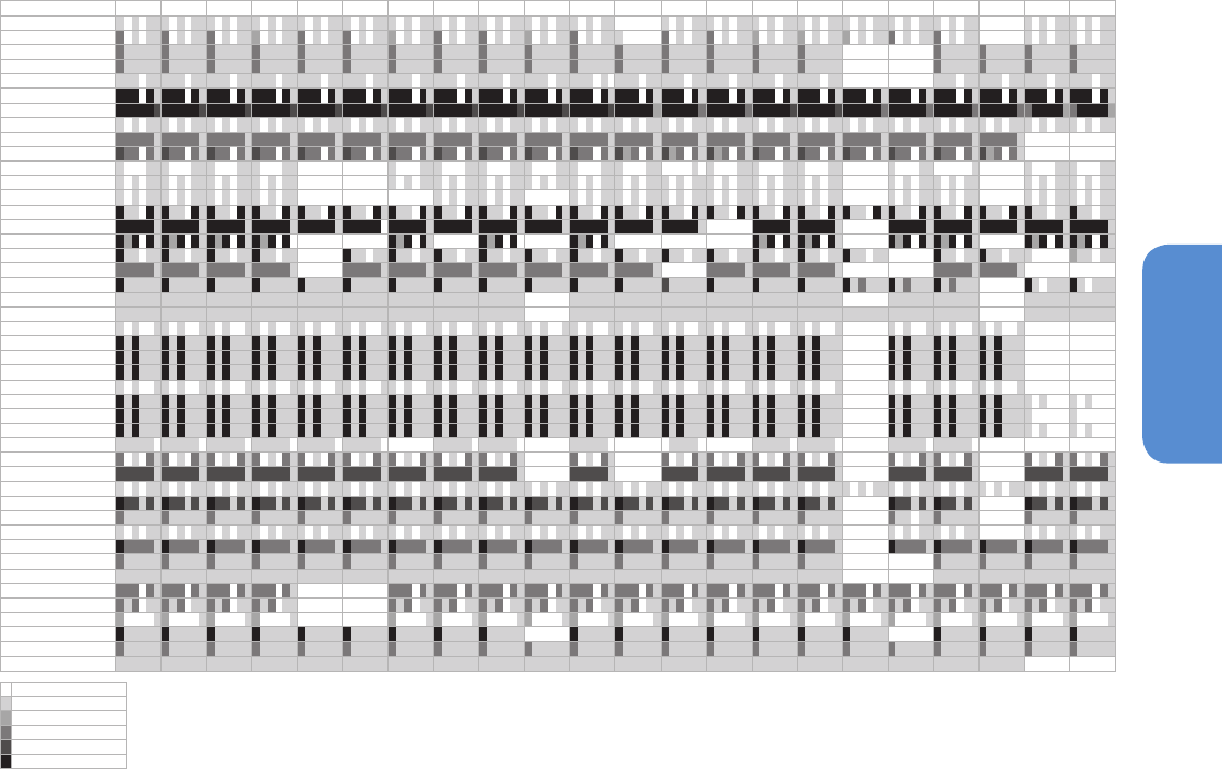
ent RCP scenarios. Figure 12.1 gives a summary of which output was

available from which model for which scenario. Where multiple runs

Model/Variable taspsl pr clthurshussevspsbl rsut rlut rtmt rsdt mrro mrso tsltauamsft.yz sossic snctas_day pr_day

ACCESS1-0

ACCESS1-3

bcc-csm1-1

bcc-csm1-1-m

BNU-ESM

CanESM2

CCSM4

CESM1-BGC

CESM1-CAM5

CESM1-WACCM

CMCC-CESM

CMCC-CM

CMCC-CMS

CNRM-CM5

CSIRO-Mk3-6-0

EC-EARTH

FGOALS-g2

FIO-ESM

GFDL-CM3

GFDL-ESM2G

GFDL-ESM2M

GISS-E2-H-CC

GISS-E2-H-P1

GISS-E2-H-P2

GISS-E2-H-P3

GISS-E2-R-CC

GISS-E2-R-P1

GISS-E2-R-P2

GISS-E2-R-P3

HadGEM2-AO

HadGEM2-CC

HadGEM2-ES

inmcm4

IPSL-CM5A-LR

IPSL-CM5A-MR

IPSL-CM5B-LR

MIROC5

MIROC-ESM

MIROC-ESM-CHEM

MPI-ESM-LR

MPI-ESM-MR

MPI-ESM-P

MRI-CGCM3

NorESM1-M

NorESM1-ME

0 ensemble

1 ensemble

2 ensembles

3 ensembles

4 ensembles

5 or more ensembles

Figure 12.1 | A summary of the output used to make the CMIP5 ﬁgures in this chapter (and some ﬁgures in Chapter 11). The climate variable names run along the horizontal axis

and use the standard abbreviations in the CMIP5 protocol (Taylor et al., 2012, and online references therein). The climate model names run along the vertical axis. In each box the

shading indicates the number of ensemble members available for historical, RCP2.6, RCP4.5, RCP6.0, RCP8.5 and pre-industrial control experiments, although only one ensemble

member per model is used in the relevant ﬁgures.

are performed with exactly the same model but with different initial

conditions, we choose only one ensemble member (usually the ﬁrst but

in cases where that was not available, the ﬁrst available member is

chosen) in order not to weight models with more ensemble members

than others unduly in the multi-model synthesis. Rather than give an

exhaustive account of which models were used to make which ﬁgures,

this summary information is presented as a guide to readers.

In addition to output from CMIP5, information from a coordinated

set of simulations with EMICs is also used (Zickfeld et al., 2013) to

investigate long-term climate change beyond 2100. Even more sim-

pliﬁed energy balance models or emulation techniques are also used,

mostly to estimate responses where ESM experiments are not availa-

ble (Meinshausen et al., 2011a; Good et al., 2013). An evaluation of

the models used for projections is provided in Chapter 9 of this Report.

12.2.2 General Concepts: Sources of Uncertainties

The understanding of the sources of uncertainty affecting future cli-

mate change projections has not substantially changed since AR4, but

many experiments and studies since then have proceeded to explore

and characterize those uncertainties further. A full characterization,

1036

Chapter 12 Long-term Climate Change: Projections, Commitments and Irreversibility

Frequently Asked Questions

FAQ 12.1 | Why Are So Many Models and Scenarios Used to Project Climate Change?

Future climate is partly determined by the magnitude of future emissions of greenhouse gases, aerosols and other

natural and man-made forcings. These forcings are external to the climate system, but modify how it behaves.

Future climate is shaped by the Earth’s response to those forcings, along with internal variability inherent in the

climate system. A range of assumptions about the magnitude and pace of future emissions helps scientists develop

different emission scenarios, upon which climate model projections are based. Different climate models, mean-

while, provide alternative representations of the Earth’s response to those forcings, and of natural climate variabil-

ity. Together, ensembles of models, simulating the response to a range of different scenarios, map out a range of

possible futures, and help us understand their uncertainties.

Predicting socioeconomic development is arguably even more difﬁcult than predicting the evolution of a physical

system. It entails predicting human behaviour, policy choices, technological advances, international competition

and cooperation. The common approach is to use scenarios of plausible future socioeconomic development, from

which future emissions of greenhouse gases and other forcing agents are derived. It has not, in general, been pos-

sible to assign likelihoods to individual forcing scenarios. Rather, a set of alternatives is used to span a range of

possibilities. The outcomes from different forcing scenarios provide policymakers with alternatives and a range of

possible futures to consider.

Internal ﬂuctuations in climate are spontaneously generated by interactions between components such as the

atmosphere and the ocean. In the case of near-term climate change, they may eclipse the effect of external per-

turbations, like greenhouse gas increases (see Chapter 11). Over the longer term, however, the effect of external

forcings is expected to dominate instead. Climate model simulations project that, after a few decades, different

scenarios of future anthropogenic greenhouse gases and other forcing agents—and the climate system’s response

to them—will differently affect the change in mean global temperature (FAQ 12.1, Figure 1, left panel). Therefore,

evaluating the consequences of those various scenarios and responses is of paramount importance, especially when

policy decisions are considered.

Climate models are built on the basis of the physical principles governing our climate system, and empirical under-

standing, and represent the complex, interacting processes needed to simulate climate and climate change, both

past and future. Analogues from past observations, or extrapolations from recent trends, are inadequate strategies

for producing projections, because the future will not necessarily be a simple continuation of what we have seen

thus far.

Although it is possible to write down the equations of ﬂuid motion that determine the behaviour of the atmo-

sphere and ocean, it is impossible to solve them without using numerical algorithms through computer model

simulation, similarly to how aircraft engineering relies on numerical simulations of similar types of equations. Also,

many small-scale physical, biological and chemical processes, such as cloud processes, cannot be described by those

equations, either because we lack the computational ability to describe the system at a ﬁne enough resolution

to directly simulate these processes or because we still have a partial scientiﬁc understanding of the mechanisms

driving these processes. Those need instead to be approximated by so-called parameterizations within the climate

models, through which a mathematical relation between directly simulated and approximated quantities is estab-

lished, often on the basis of observed behaviour.

There are various alternative and equally plausible numerical representations, solutions and approximations for

modelling the climate system, given the limitations in computing and observations. This diversity is considered a

healthy aspect of the climate modelling community, and results in a range of plausible climate change projections

at global and regional scales. This range provides a basis for quantifying uncertainty in the projections, but because

the number of models is relatively small, and the contribution of model output to public archives is voluntary,

the sampling of possible futures is neither systematic nor comprehensive. Also, some inadequacies persist that are

common to all models; different models have different strength and weaknesses; it is not yet clear which aspects

of the quality of the simulations that can be evaluated through observations should guide our evaluation of future

model simulations. (continued on next page)

1037

Long-term Climate Change: Projections, Commitments and Irreversibility Chapter 12

FAQ 12.1 (continued)

Models of varying complexity are commonly used for different projection problems. A faster model with lower

resolution, or a simpliﬁed description of some climate processes, may be used in cases where long multi-century

simulations are required, or where multiple realizations are needed. Simpliﬁed models can adequately represent

large-scale average quantities, like global average temperature, but ﬁner details, like regional precipitation, can be

simulated only by complex models.

The coordination of model experiments and output by groups such as the Coupled Model Intercomparison Project

(CMIP), the World Climate Research Program and its Working Group on Climate Models has seen the science com-

munity step up efforts to evaluate the ability of models to simulate past and current climate and to compare future

climate change projections. The ‘multi-model’ approach is now a standard technique used by the climate science

community to assess projections of a speciﬁc climate variable.

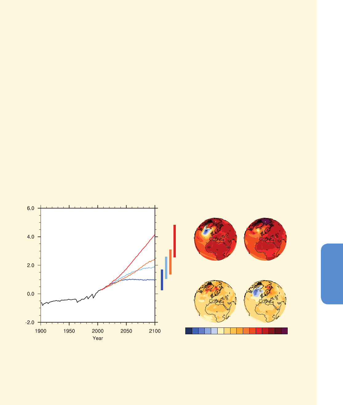
FAQ 12.1, Figure 1, right panels, shows the temperature response by the end of the 21st century for two illustrative

models and the highest and lowest RCP scenarios. Models agree on large-scale patterns of warming at the surface,

for example, that the land is going to warm faster than ocean, and the Arctic will warm faster than the tropics. But

they differ both in the magnitude of their global response for the same scenario, and in small scale, regional aspects

of their response. The magnitude of Arctic ampliﬁcation, for instance, varies among different models, and a subset

of models show a weaker warming or slight cooling in the North Atlantic as a result of the reduction in deepwater

formation and shifts in ocean currents.

There are inevitable uncertainties in future external forcings, and the climate system’s response to them, which

are further complicated by internally generated variability. The use of multiple scenarios and models have become

a standard choice in order to assess and characterize them, thus allowing us to describe a wide range of possible

future evolutions of the Earth’s climate.

FAQ 12.1, Figure 1 | Global mean temperature change averaged across all Coupled Model Intercomparison Project Phase 5 (CMIP5) models (relative to 1986–2005)

for the four Representative Concentration Pathway (RCP) scenarios: RCP2.6 (dark blue), RCP4.5 (light blue), RCP6.0 (orange) and RCP8.5 (red); 32, 42, 25 and 39

models were used respectively for these 4 scenarios. Likely ranges for global temperature change by the end of the 21st centuryare indicated by vertical bars. Note that

these ranges apply to the difference between two 20-year means, 2081–2100 relative to 1986–2005, which accounts for the bars being centred at a smaller value than

the end point of the annual trajectories. For the highest (RCP8.5) and lowest (RCP2.6) scenario, illustrative maps of surface temperature change at the end of the 21st

century (2081–2100 relative to 1986–2005) are shown for two CMIP5 models. These models are chosen to show a rather broad range of response, but this particular

set is not representative of any measure of model response uncertainty.

Model mean global

mean temperature

change for high

emission scenario

RCP8.5

Model mean global

mean temperature

change for low

emission scenario

RCP2.6

Global surface temperature change (°C)

Possible temperature responses in 2081-2100 to

high emission scenario RCP8.5

Possible temperature responses in 2081-2100 to

low emission scenario RCP2.6

-2 -1.5 -1-0.5 00.5 11.5 23457911

(°C)

1038

Chapter 12 Long-term Climate Change: Projections, Commitments and Irreversibility

qualitative and even more so quantitative, involves much more than a

measure of the range of model outcomes, because additional sources

of information (e.g., observational constraints, model evaluation, expert

judgement) lead us to expect that the uncertainty around the future

climate state does not coincide straightforwardly with those ranges.

In fact, in this chapter we highlight wherever relevant the distinction

between model uncertainty evaluation, which encompasses the under-

standing that models have intrinsic shortcoming in fully and accurately

representing the real system, and cannot all be considered independent

of one another (Knutti et al., 2013), and a simpler descriptive quantiﬁ-

cation, based on the range of outcomes from the ensemble of models.

Uncertainty affecting mid- to long-term projections of climatic changes

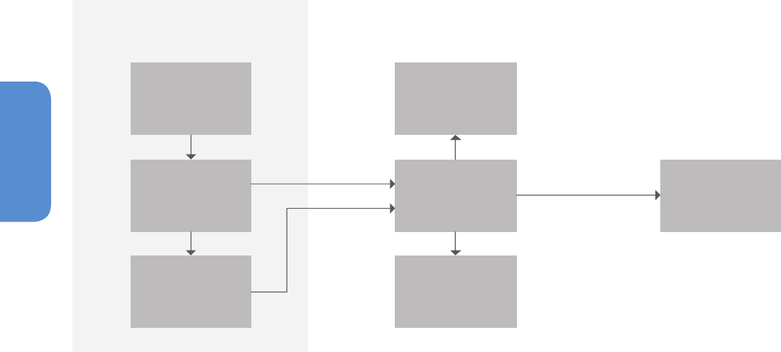
stems from distinct but possibly interacting sources. Figure 12.2 shows

a schematic of the chain from scenarios, through ESMs to projections.

Uncertainties affecting near-term projections of which some aspect

are also relevant for longer-term projections are discussed in Section

11.3.1.1 and shown in Figure 11.8.

Future anthropogenic emissions of GHGs, aerosol particles and other

forcing agents such as land use change are dependent on socioec-

onomic factors including global geopolitical agreements to control

those emissions. Systematic studies that attempt to quantify the likely

ranges of anthropogenic emission have been undertaken (Sokolov et

al., 2009) but it is more common to use a scenario approach of dif-

ferent but plausible—in the sense of technically feasible—pathways,

leading to the concept of scenario uncertainty. AR4 made extensive

use of the SRES scenarios (IPCC, 2000) developed using a sequential

approach, that is, socioeconomic factors feed into emissions scenarios

which are then used either to directly force the climate models or to

determine concentrations of GHGs and other agents required to drive

these models. This report also assesses outcomes of simulations that

use the new RCP scenarios, developed using a parallel process (Moss

et al., 2010) whereby different targets in terms of RF at 2100 were

selected (2.6, 4.5, 6.0 and 8.5 W m

–2

) and GHG and aerosol emissions

consistent with those targets, and their corresponding socioeconom-

ic drivers were developed simultaneously (see Section 12.3). Rather

than being identiﬁed with one socioeconomic storyline, RCP scenarios

are consistent with many possible economic futures (in fact, different

combinations of GHG and aerosol emissions can lead to the same

RCP). Their development was driven by the need to produce scenari-

os that could be input to climate model simulations more expediently

while corresponding socioeconomic scenarios would be developed in

parallel, and to produce a wide range of model responses that may be

scaled and interpolated to estimate the response under other scenari-

os, involving different measures of adaptation and mitigation.

In terms of the uncertainties related to the RCP emissions scenarios,

the following issues can be identiﬁed:

• No probabilities or likelihoods have been attached to the alterna-

tive RCP scenarios (as was the case for SRES scenarios). Each of

them should be considered plausible, as no study has questioned

their technical feasibility (see Chapter 1).

Target Radiative

Forcing

Concentrations

Emissions

Diagnosed Radiative

Forcing

Earth System

Models

Diagnosed

Emissions

Climate Projections

Representative

Concentration Pathway (RCP)

Figure 12.2 | Links in the chain from scenarios, through models to climate projections. The Representative Concentration Pathways (RCPs) are designed to sample a range of

radiative forcing (RF) of the climate system at 2100. The RCPs are translated into both concentrations and emissions of greenhouse gases using Integrated Assessment Models

(IAMs). These are then used as inputs to dynamical Earth System Models (ESMs) in simulations that are either concentration-driven (the majority of projection experiments) or

emissions-driven (only for RCP8.5). Aerosols and other forcing factors are implemented in different ways in each ESM. The ESM projections each have a potentially different RF,

which may be viewed as an output of the model and which may not correspond to precisely the level of RF indicated by the RCP nomenclature. Similarly, for concentration-driven

experiments, the emissions consistent with those concentrations diagnosed from the ESM may be different from those speciﬁed in the RCP (diagnosed from the IAM). Different

models produce different responses even under the same RF. Uncertainty propagates through the chain and results in a spread of ESM projections. This spread is only one way

of assessing uncertainty in projections. Alternative methods, which combine information from simple and complex models and observations through statistical models or expert

judgement, are also used to quantify that uncertainty.

1039

Long-term Climate Change: Projections, Commitments and Irreversibility Chapter 12

• Despite the naming of the RCPs in terms of their target RF at 2100

or at stabilization (Box 1.1), climate models translate concentra-

tions of forcing agents into RF in different ways due to their differ-

ent structural modelling assumptions. Hence a model simulation

of RCP6.0 may not attain exactly a RF of 6 W m

–2

; more accurately,

an RCP6.0 forced model experiment may not attain exactly the

same RF as was intended by the speciﬁcation of the RCP6.0 forc-

ing inputs. Thus in addition to the scenario uncertainty there is

RF uncertainty in the way the RCP scenarios are implemented in

climate models.

• Some model simulations are concentration-driven (GHG concen-

trations are speciﬁed) whereas some models, which have Earth

Systems components, convert emission scenarios into concen-

trations and are termed emissions-driven. Different ESMs driven

by emissions may produce different concentrations of GHGs and

aerosols because of differences in the representation and/or

parameterization of the processes responsible for the conversion

of emissions into concentrations. This aspect may be considered a

facet of forcing uncertainty, or may be compounded in the category

of model uncertainty, which we discuss below. Also, aerosol load-

ing and land use changes are not dictated intrinsically by the RCP

speciﬁcation. Rather, they are a result of the Integrated Assessment

Model that created the emission pathway for a given RCP.

SRES and RCPs account for future changes only in anthropogenic forc-

ings. With regard to solar forcing, the 1985–2005 solar cycle is repeat-

ed. Neither projections of future deviations from this solar cycle, nor

future volcanic RF and their uncertainties are considered.

Any climate projection is subject to sampling uncertainties that arise

because of internal variability. In this chapter, the prediction of, for

example, the amplitude or phase of some mode of variability that may

be important on long time scales is not addressed (see Sections 11.2

and 11.3). Any climate variable projection derived from a single simu-

lation of an individual climate model will be affected by internal varia-

bility (stemming from the chaotic nature of the system), whether it be

a variable that involves a long time average (e.g., 20 years), a snapshot

in time or some more complex diagnostic such as the variance comput-

ed from a time series over many years. No amount of time averaging

can reduce internal variability to zero, although for some EMICs and

simpliﬁed models, which may be used to reproduce the results of more

complex model simulations, the representation of internal variability

is excluded from the model speciﬁcation by design. For different

variables, and different spatial and time scale averages, the relative

importance of internal variability in comparison with other sources of

uncertainty will be different. In general, internal variability becomes

more important on shorter time scales and for smaller scale variables

(see Section 11.3 and Figure 11.2). The concept of signal-to-noise ratio

may be used to quantify the relative magnitude of the forced response

(signal) versus internal variability (noise). Internal variability may be

sampled and estimated explicitly by running ensembles of simulations

with slightly different initial conditions, designed explicitly to represent

internal variability, or can be estimated on the basis of long control

runs where external forcings are held constant. In the case of both

multi-model and perturbed physics ensembles (see below), there is an

implicit perturbation in the initial state of each run considered, which

means that these ensembles sample both modelling uncertainty and

internal variability jointly.

The ability of models to mimic nature is achieved by simpliﬁcation

choices that can vary from model to model in terms of the fundamental

numeric and algorithmic structures, forms and values of parameteriza-

tions, and number and kinds of coupled processes included. Simpliﬁ-

cations and the interactions between parameterized and resolved pro-

cesses induce ‘errors’ in models, which can have a leading-order impact

on projections. It is possible to characterize the choices made when

building and running models into structural—indicating the numerical

techniques used for solving the dynamical equations, the analytic form

of parameterization schemes and the choices of inputs for ﬁxed or var-

ying boundary conditions—and parametric—indicating the choices

made in setting the parameters that control the various components

of the model. The community of climate modellers has regularly col-

laborated in producing coordinated experiments forming multi-model

ensembles (MMEs), using both global and regional model families, for

example, CMIP3/5 (Meehl et al., 2007a), ENSEMBLES (Johns et al.,

2011) and Chemistry–Climate Model Validation 1 and 2 (CCM-Val-1

and 2; Eyring et al., 2005), through which structural uncertainty can be

at least in part explored by comparing models, and perturbed physics

ensembles (PPEs, with e.g., Hadley Centre Coupled Model version 3

(HadCM3; Murphy et al., 2004), Model for Interdiciplinary Research On

Climate (MIROC; Yokohata et al., 2012), Community Climate System

Model 3 (CCSM3; Jackson et al., 2008; Sanderson, 2011)), through

which uncertainties in parameterization choices can be assessed in a

given model. As noted below, neither MMEs nor PPEs represent an

adequate sample of all the possible choices one could make in building

a climate model. Also, current models may exclude some processes that

could turn out to be important for projections (e.g., methane clathrate

release) or produce a common error in the representation of a particu-

lar process. For this reason, it is of critical importance to distinguish

two different senses in which the uncertainty terminology is used or

misused in the literature (see also Sections 1.4.2, 9.2.2, 9.2.3, 11.2.1

and 11.2.2). A narrow interpretation of the concept of model uncer-

tainty often identiﬁes it with the range of responses of a model ensem-

ble. In this chapter this type of characterization is referred as model

range or model spread. A broader concept entails the recognition of a

fundamental uncertainty in the representation of the real system that

these models can achieve, given their necessary approximations and

the limits in the scientiﬁc understanding of the real system that they

encapsulate. When addressing this aspect and characterizing it, this

chapter uses the term model uncertainty.

The relative role of the different sources of uncertainty—model, sce-

nario and internal variability—as one moves from short- to mid- to

long-term projections and considers different variables at different

spatial scales has to be recognized (see Section 11.3). The three sourc-

es exchange relevance as the time horizon, the spatial scale and the

variable change. In absolute terms, internal variability is generally

estimated, and has been shown in some speciﬁc studies (Hu et al.,

2012) to remain approximately constant across the forecast horizon,

with model ranges and scenario/forcing variability increasing over

time. For forecasts of global temperatures after mid-century, scenario

and model ranges dominate the amount of variation due to internally

generated variability, with scenarios accounting for the largest source

1040

Chapter 12 Long-term Climate Change: Projections, Commitments and Irreversibility

of uncertainty in projections by the end of the century. For global aver-

age precipitation projections, scenario uncertainty has a much smaller

role even by the end of the 21st century and model range maintains

the largest share across all projection horizons. For temperature and

precipitation projections at smaller spatial scales, internal variability

may remain a signiﬁcant source of uncertainty up until middle of the

21st century in some regions (Hawkins and Sutton, 2009, 2011; Rowell,

2012; Knutti and Sedláček, 2013). Within single model experiments,

the persistently signiﬁcant role of internally generated variability for

regional projections even beyond short- and mid-term horizons has

been documented by analyzing relatively large ensembles sampling

initial conditions (Deser et al., 2012a, 2012b).

12.2.3 From Ensembles to Uncertainty Quantiﬁcation

Ensembles like CMIP5 do not represent a systematically sampled

family of models but rely on self-selection by the modelling groups.

This opportunistic nature of MMEs has been discussed, for example, in

Tebaldi and Knutti (2007) and Knutti et al. (2010a). These ensembles are

therefore not designed to explore uncertainty in a coordinated manner,

and the range of their results cannot be straightforwardly interpreted

as an exhaustive range of plausible outcomes, even if some studies

have shown how they appear to behave as well calibrated probabil-

istic forecasts for some large-scale quantities (Annan and Hargreaves,

2010). Other studies have argued instead that the tail of distributions

is by construction undersampled (Räisänen, 2007). In general, the dif-

ﬁculty in producing quantitative estimates of uncertainty based on

multiple model output originates in their peculiarities as a statistical

sample, neither random nor systematic, with possible dependencies

among the members (Jun et al., 2008; Masson and Knutti, 2011; Pen-

nell and Reichler, 2011; Knutti et al., 2013) and of spurious nature, that

is, often counting among their members models with different degrees

of complexities (different number of processes explicitly represented or

parameterized) even within the category of general circulation models.

Agreement between multiple models can be a source of information in

an uncertainty assessment or conﬁdence statement. Various methods

have been proposed to indicate regions where models agree on the

projected changes, agree on no change or disagree. Several of those

methods are compared in Box 12.1. Many ﬁgures use stippling or

hatching to display such information, but it is important to note that

conﬁdence cannot be inferred from model agreement alone.

Perturbed physics experiments (PPEs) differ in their output interpret-

ability for they can be, and have been, systematically constructed

and as such lend themselves to a more straightforward treatment

through statistical modelling (Rougier, 2007; Sanso and Forest, 2009).

Uncertain parameters in a single model to whose values the output

is known to be sensitive are targeted for perturbations. More often

it is the parameters in the atmospheric component of the model that

are varied (Collins et al., 2006a; Sanderson et al., 2008), and to date

have in fact shown to be the source of the largest uncertainties in

large-scale response, but lately, with much larger computing power

expense, also parameters within the ocean component have been per-

turbed (Collins et al., 2007; Brierley et al., 2010). Parameters in the

land surface schemes have also been subject to perturbation studies

(Fischer et al., 2011; Booth et al., 2012; Lambert et al., 2012). Ranges

of possible values are explored and often statistical models that ﬁt the

relationship between parameter values and model output, that is, emu-

lators, are trained on the ensemble and used to predict the outcome

for unsampled parameter value combinations, in order to explore the

parameter space more thoroughly that would otherwise be computa-

tionally affordable (Rougier et al., 2009). The space of a single model

simulations (even when ﬁltered through observational constraints) can

show a large range of outcomes for a given scenario (Jackson et al.,

2008). However, multi-model ensembles and perturbed physics ensem-

bles produce modes and distributions of climate responses that can

be different from one another, suggesting that one type of ensemble

cannot be used as an analogue for the other (Murphy et al., 2007;

Sanderson et al., 2010; Yokohata et al., 2010; Collins et al., 2011).

Many studies have made use of results from these ensembles to charac-

terize uncertainty in future projections, and these will be assessed and

their results incorporated when describing speciﬁc aspects of future

climate responses. PPEs have been uniformly treated across the differ-

ent studies through the statistical framework of analysis of computer

experiments (Sanso et al., 2008; Rougier et al., 2009; Harris et al., 2010)

or, more plainly, as a thorough exploration of alternative responses

reweighted by observational constraints (Murphy et al., 2004; Piani et

al., 2005; Forest et al., 2008; Sexton et al., 2012). In all cases the con-

struction of a probability distribution is facilitated by the systematic

nature of the experiments. MMEs have generated a much more diver-

siﬁed treatment (1) according to the choice of applying weights to the

different models on the basis of past performance or not (Weigel et al.,

2010) and (2) according to the choice between treating the different

models and the truth as indistinguishable or treating each model as

a version of the truth to which an error has been added (Annan and

Hargreaves, 2010; Sanderson and Knutti, 2012). Many studies can be

classiﬁed according to these two criteria and their combination, but

even within each of the four resulting categories different studies pro-

duce different estimates of uncertainty, owing to the preponderance

of a priori assumptions, explicitly in those studies that approach the

problem through a Bayesian perspective, or only implicit in the choice

of likelihood models, or weighting. This makes the use of probabilistic

and other results produced through statistical inference necessarily

dependent on agreeing with a particular set of assumptions (Sansom

et al., 2013), given the lack of a full exploration of the robustness of

probabilistic estimates to varying these assumptions.

In summary, there does not exist at present a single agreed on and

robust formal methodology to deliver uncertainty quantiﬁcation esti-

mates of future changes in all climate variables (see also Section 9.8.3

and Stephenson et al., 2012). As a consequence, in this chapter, state-

ments using the calibrated uncertainty language are a result of the

expert judgement of the authors, combining assessed literature results

with an evaluation of models demonstrated ability (or lack thereof)

in simulating the relevant processes (see Chapter 9) and model con-

sensus (or lack thereof) over future projections. In some cases when a

signiﬁcant relation is detected between model performance and relia-

bility of its future projections, some models (or a particular parametric

conﬁguration) may be excluded (e.g., Arctic sea ice; Section 12.4.6.1

and Joshi et al., 2010) but in general it remains an open research ques-

tion to ﬁnd signiﬁcant connections of this kind that justify some form

of weighting across the ensemble of models and produce aggregated

1041

Long-term Climate Change: Projections, Commitments and Irreversibility Chapter 12

Box 12.1 | Methods to Quantify Model Agreement in Maps

The climate change projections in this report are based on ensembles of climate models. The ensemble mean is a useful quantity to

characterize the average response to external forcings, but does not convey any information on the robustness of this response across

models, its uncertainty and/or likelihood or its magnitude relative to unforced climate variability. In the IPCC AR4 WGI contribution

(IPCC, 2007) several criteria were used to indicate robustness of change, most prominently in Figure SPM.7. In that ﬁgure, showing

projected precipitation changes, stippling marked regions where at least 90% of the CMIP3 models agreed on the sign of the change.

Regions where less than 66% of the models agreed on the sign were masked white. The resulting large white area was often misin-

terpreted as indicating large uncertainties in the different models’ response to external forcings, but recent studies show that, for the

most part, the disagreement in sign among models is found where projected changes are small and still within the modelled range

of internal variability, that is, where a response to anthropogenic forcings has not yet emerged locally in a statistically signiﬁcant way

(Tebaldi et al., 2011; Power et al., 2012).

A number of methods to indicate model robustness, involving an assessment of the signiﬁcance of the change when compared to inter-

nal variability, have been proposed since AR4. The different methods share the purpose of identifying regions with large, signiﬁcant or

robust changes, regions with small changes, regions where models disagree or a combination of those. They do, however, use different

assumptions about the statistical properties of the model ensemble, and therefore different criteria for synthesizing the information

from it. Different methods also differ in the way they estimate internal variability. We brieﬂy describe and compare several of these

methods here.

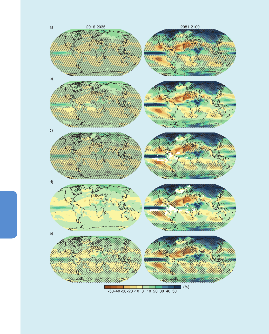
Method (a): The default method used in Chapters 11,12 and 14 as well as in the Annex I (hatching only) is shown in Box 12.1, Figure

1a, and is based on relating the climate change signal to internal variability in 20-year means of the models as a reference

. Regions

where the multi-model mean change exceeds two standard deviations of internal variability and where at least 90% of the models

agree on the sign of change are stippled and interpreted as ‘large change with high model agreement’. Regions where the model mean

is less than one standard deviation of internal variability are hatched and interpreted as ‘small signal or low agreement of models’. This

can have various reasons: (1) changes in individual models are smaller than internal variability, or (2) although changes in individual

models are signiﬁcant, they disagree about the sign and the multi-model mean change remains small. Using this method, the case

where all models scatter widely around zero and the case where all models agree on near zero change therefore are both hatched

(e.g., precipitation change over the Amazon region by the end of the 21st century, which the following methods mark as ‘inconsistent

model response’).

Method (b): Method (a) does not distinguish the case where all models agree on no change and the case where, for example, half of

the models show a signiﬁcant increase and half a decrease. The distinction may be relevant for many applications and a modiﬁcation

of method (a) is to restrict hatching to regions where there is high agreement among the models that the change will be ‘small’, thus

eliminating the ambiguous interpretation ‘small or low agreement’ in (a). In contrast to method (a) where the model mean is com-

pared to variability, this case (b) marks regions where at least 80% of the individual models show a change smaller than two standard

deviations of variability with hatching. Grid points where many models show signiﬁcant change but don’t agree are no longer hatched

(Box 12.1, Figure 1b).

Method (c): Knutti and Sedláček (2013) deﬁne a dimensionless robustness measure, R, which is inspired by the signal-to-noise ratio

and the ranked probability skill score. It considers the natural variability and agreement on magnitude and sign of change. A value of

R = 1 implies perfect model agreement; low or negative values imply poor model agreement (note that by deﬁnition R can assume any

negative value). Any level of R can be chosen for the stippling. For illustration, in Box 12.1, Figure 1c, regions with R > 0.8 are marked

with small dots, regions with R > 0.9 with larger dots and are interpreted as ‘robust large change’. This yields similar results to method

(a) for the end of the century, but with some areas of moderate model robustness (R > 0.8) already for the near-term projections,

even though the signal is still within the noise. Regions where at least 80% of the models individually show no signiﬁcant change

are hatched and interpreted as ‘changes unlikely to emerge from variability’

.There is less hatching in this method than in method (a),

The internal variability in this method is estimated using pre-industrial control runs for each of the models which are at least 500 years long. The ﬁrst 100 years of

the pre-industrial are ignored. Variability is calculated for every grid point as the standard deviation of non-overlapping 20-year means, multiplied by the square

root of 2 to account for the fact that the variability of a difference in means is of interest. A quadratic ﬁt as a function of time is subtracted from these at every grid

point to eliminate model drift. This is by deﬁnition the standard deviation of the difference between two independent 20-year averages having the same variance

and estimates the variation of that difference that would be expected due to unforced internal variability. The median across all models of that quantity is used.

Variability in methods b–d is estimated from interannual variations in the base period within each model.

(continued on next page)

1042

Chapter 12 Long-term Climate Change: Projections, Commitments and Irreversibility

DJF mean precipitation change (RCP8.5)

Box 12.1, Figure 1 | Projected change in December to February precipitation for 2016–2035 and 2081–2100, relative to 1986–2005 from CMIP5 models. The

choice of the variable and time frames is just for illustration of how the different methods compare in cases with low and high signal-to-noise ratio (left and right

column, respectively). The colour maps are identical along each column and only stippling and hatching differ on the basis of the different methods. Different methods

for stippling and hatching are shown determined (a) from relating the model mean to internal variability, (b) as in (a) but hatching here indicates high agreement for

‘small change’, (c) by the robustness measure by Knutti and Sedláček (2013), (d) by the method proposed by Tebaldi et al. (2011) and (e) by the method by Power et

al. (2012). Detailed technical explanations for each method are given in the text. 39 models are used in all panels.

Box 12.1 (continued)

1043

Long-term Climate Change: Projections, Commitments and Irreversibility Chapter 12

Box 12.1 (continued)

because it requires 80% of the models to be within variability, not just the model average. Regions where at least 50% of the models

show signiﬁcant change but R< 0.5 are masked as white to indicate ‘models disagreeing on the projected change projections’ (Box

12.1, Figure 1c).

Method (d): Tebaldi et al. (2011) start from IPCC AR4 SPM7 but separate lack of model agreement from lack of signal (Box 12.1, Figure

1e). Grid points are stippled and interpreted as ‘robust large change’ when more than 50% of the models show signiﬁcant change and

at least 80% of those agree on the sign of change. Grid points where more than 50% of the models show signiﬁcant change but less

than 80% of those agree on the sign of change are masked as white and interpreted as ‘unreliable’. The results are again similar to

the methods above. No hatching was deﬁned in that method (Box 12.1 Figure 1d). (See also Neelin et al., 2006 for a similar approach

applied to a speciﬁc regional domain.)

Method (e): Power et al. (2012) identify three distinct regions using various methods in which projections can be very loosely described

as either: ‘statistically signiﬁcant’, ‘small (relative to temporal variability) or zero, but not statistically signiﬁcant’ or ‘uncertain’. The

emphasis with this approach is to identify robust signals taking the models at face value and to address the questions: (1) What

will change? (2) By how much? and (3) What will not change? The underlying consideration here is that statistical testing under the

assumption of model independence provides a worthwhile, albeit imperfect, line of evidence that needs to be considered in conjunction

with other evidence (e.g., degree of interdependence, ability of models to simulate the past), in order to assess the degree of conﬁdence

one has in a projected change.

The examples given here are not exhaustive but illustrate the main ideas. Other methods include simply counting the number of models

agreeing on the sign (Christensen et al., 2007), or varying colour hue and saturation to indicate magnitude of change and robustness

of change separately (Kaye et al., 2012). In summary, there are a variety of ways to characterize magnitude or signiﬁcance of change,

and agreement between models. There is also a compromise to make between clarity and richness of information. Different methods

serve different purposes and a variety of criteria can be justiﬁed to highlight speciﬁc properties of multi-model ensembles. Clearly only

a subset of information regarding robust and uncertain change can be conveyed in a single plot. The methods above convey some

important pieces of this information, but obviously more information could be provided if more maps with additional statistics were

provided. In fact Annex I provides more explicit information on the range of projected changes evident in the models (e.g., the median,

and the upper and lower quartiles). For most of the methods there is a necessity to choose thresholds for the level of agreement that

cannot be identiﬁed objectively, but could be the result of individual, application-speciﬁc evaluations. Note also that all of the above

methods measure model agreement in an ensemble of opportunity, and it is impossible to derive a conﬁdence or likelihood statement

from the model agreement or model spread alone, without considering consistency with observations, model dependence and the

degree to which the relevant processes are understood and reﬂected in the models (see Section 12.2.3).

The method used by Power et al. (2012) differs from the other methods in that it tests the statistical signiﬁcance of the ensemble mean

rather than a single simulation. As a result, the area where changes are signiﬁcant increases with an increasing number of models.

Already for the period centred on 2025, most of the grid points when using this method show signiﬁcant change in the ensemble

mean whereas in the other methods projections for this time period are classiﬁed as changes not exceeding internal variability. The

reason is that the former produces a statement about the mean of the distribution being signiﬁcantly different from zero, equivalent to

treating the ensemble as ‘truth plus error’, that is, assuming that the models are independent and randomly distributed around reality.

Methods a–d, on the other hand, use an ‘indistinguishable’ interpretation, in which each model and reality are drawn from the same

distribution. In that case, the stippling and hatching characterize the likelihood of a single member being signiﬁcant or not, rather than

the ensemble mean. There is some debate in the literature on how the multi-model ensembles should be interpreted statistically. This

and past IPCC reports treat the model spread as some measure of uncertainty, irrespective of the number of models, which implies an

‘indistinguishable’ interpretation. For a detailed discussion readers are referred to the literature (Tebaldi and Knutti, 2007; Annan and

Hargreaves, 2010; Knutti et al., 2010a, 2010b; Annan and Hargreaves, 2011a; Sanderson and Knutti, 2012).

1044

Chapter 12 Long-term Climate Change: Projections, Commitments and Irreversibility

future projections that are signiﬁcantly different from straightforward

one model–one vote (Knutti, 2010) ensemble results. Therefore, most

of the analyses performed for this chapter make use of all available

models in the ensembles, with equal weight given to each of them

unless otherwise stated.

12.2.4 Joint Projections of Multiple Variables

While many of the key processes relevant to the simulation of single

variables are understood, studies are only starting to focus on assess-

ing projections of joint variables, especially when extremes or varia-

bility in the individual quantities are of concern. A few studies have

addressed projected changes in joint variables, for example, by combin-

ing mean temperature and precipitation (Williams et al., 2007; Tebaldi

and Lobell, 2008; Tebaldi and Sanso, 2009; Watterson, 2011; Watter-

son and Whetton, 2011a; Sexton et al., 2012), linking soil moisture,

precipitation and temperature mean and variability (Seneviratne et al.,

2006; Fischer and Schär, 2009; Koster et al., 2009b, 2009c), combining

temperature and humidity (Diffenbaugh et al., 2007; Fischer and Schär,

2010; Willett and Sherwood, 2012), linking summertime temperature

and soil moisture to prior winter snowpack (Hall et al., 2008) or linking

precipitation change to circulation, moisture and moist static energy

budget changes (Neelin et al., 2003; Chou and Neelin, 2004; Chou et

al., 2006, 2009). Models may have difﬁculties simulating all relevant

interactions between atmosphere and land surface and the water cycle

that determine the joint response, observations to evaluate models are

often limited (Seneviratne et al., 2010), and model uncertainties are

therefore large (Koster et al., 2006; Boé and Terray, 2008; Notaro, 2008;

Fischer et al., 2011). In some cases, correlations between, for example,

temperature and precipitation or accumulated precipitation and tem-

perature have found to be too strong in climate models (Trenberth and

Shea, 2005; Hirschi et al., 2011). The situation is further complicated

by the fact that model biases in one variable affect other variables.

The standard method for model projections is to subtract model biases

derived from control integrations (assuming that the bias remains con-

stant in a future scenario integration). Several studies note that this

may be problematic when a consistent treatment of biases in multiple

variables is required (Christensen et al., 2008; Buser et al., 2009), but

there is no consensus at this stage for a methodology addressing this

problem (Ho et al., 2012). More generally the existence of structural

errors in models according to which an unavoidable discrepancy (Rou-

gier, 2007) between their simulations and reality cannot be avoided

is relevant here, as well as for univariate projections. In the recent lit-

erature an estimate of this discrepancy has been proposed through

the use of MMEs, using each model in turn as a surrogate for reali-

ty, and measuring the distance between it and the other models of

the ensemble. Some summary statistic of these measures is then used

to estimate the distance between models and the real world (Sexton

and Murphy, 2012; Sexton et al., 2012; Sanderson, 2013). Statistical

frameworks to deal with multivariate projections are challenging even

for just two variables, as they have to address a trade-off between

modelling the joint behavior at scales that are relevant for impacts—

that is, ﬁne spatial and temporal scales, often requiring complex spa-

tio-temporal models—and maintaining computational feasibility. In

one instance (Tebaldi and Sanso, 2009) scales were investigated at

the seasonal and sub-continental level, and projections of the forced

response of temperature and precipitation at those scales did not show

signiﬁcant correlations, likely because of the heterogeneity of the rela-

tion between the variables within those large averaged regions and

seasons. In Sexton et al. (2012) the spatial scale focussed on regions of

Great Britain and correlation emerged as more signiﬁcant, for exam-

ple, between summer temperatures and precipitation amounts. Fischer

and Knutti (2013) estimated strong relationships between variables

making up impact relevant indices (e.g., temperature and humidi-

ty) and showed how in some cases, uncertainties across models are

larger for a combined variable than if the uncertainties in the individ-

ual underlying variables were treated independently (e.g., wildﬁres),

whereas in other cases theuncertainties in the combined variables are

smaller than in the individual ones (e.g., heat stress for humans).

Even while recognizing the need for joint multivariate projections, the

above limitations at this stage prevent a quantitative assessment for

most cases. A few robust qualitative relationships nonetheless emerge

from the literature and these are assessed, where appropriate, in the

rest of the chapter. For applications that are sensitive to relationships

between variables, but still choose to use the multi-model framework

to determine possible ranges for projections, sampling from univari-

ate ranges may lead to unrealistic results when signiﬁcant correlations

exist. IPCC assessments often show model averages as best estimates,

but such averages can underestimate spatial variability, and more in

general they neither represent any of the actual model states (Knutti et

al., 2010a) nor do they necessarily represent the joint best estimate in a

multivariate sense. Impact studies usually need temporally and spatial-

ly coherent multivariate input from climate model simulations. In those

cases, using each climate model output individually and feeding it into

the impact model, rather than trying to summarise a multivariate distri-

bution from the MME and sample from it, is likely to be more consist-

ent, assuming that the climate model itself correctly captures the spa-

tial covariance, the temporal co-evolution and the relevant feedbacks.

12.3 Projected Changes in Forcing Agents,

Including Emissions and Concentrations

The experiments that form the basis of global future projections dis-

cussed in this chapter are extensions of the simulations of the observa-

tional record discussed in Chapters 9 and 10. The scenarios assessed in

AR5, introduced in Chapter 1, include four new scenarios designed to

explore a wide range of future climate characterized by representative

trajectories of well-mixed greenhouse gas (WMGHG) concentrations

and other anthropogenic forcing agents. These are described further

in Section 12.3.1. The implementation of forcing agents in model pro-

jections, including natural and anthropogenic aerosols, ozone and land

use change are discussed in Section 12.3.2, with a strong focus on

CMIP5 experiments. Global mean emissions, concentrations and RFs

applicable to the historical record simulations assessed in Chapters 8,

9 and 10, and the future scenario simulations assessed here, are listed

in Annex II. Global mean RF for the 21st century consistent with these

scenarios, derived from CMIP5 and other climate model studies, is dis-

cussed in Section 12.3.3.

1045

Long-term Climate Change: Projections, Commitments and Irreversibility Chapter 12

12.3.1 Description of Scenarios

Long-term climate change projections reﬂect how human activities or

natural effects could alter the climate over decades and centuries. In

this context, deﬁned scenarios are important, as using speciﬁc time

series of emissions, land use, atmospheric concentrations or RF across

multiple models allows for coherent climate model intercomparisons

and synthesis. Some scenarios present a simple stylized future (not

accompanied by a socioeconomic storyline) and are used for pro-

cess understanding. More comprehensive scenarios are produced by

Integrated Assessment Models (IAMs) as internally consistent sets of

emissions and socioeconomic assumptions (e.g., regarding population

and socioeconomic development) with the aim of presenting sever-

al plausible future worlds (see Section 1.5.2 and Box 1.1). In general

it is these scenarios that are used for policy relevant climate change,

impact, adaptation and mitigation analysis. It is beyond the scope of

this report to consider the full range of currently published scenarios

and their implications for mitigation policy and climate targets—that

is covered by the Working Group III contribution to the AR5. Here, we

focus on the RCP scenarios used within the CMIP5 intercomparison

exercise (Taylor et al. 2012) along with the SRES scenarios (IPCC, 2000)

developed for the IPCC Third Assessment Report (TAR) but still widely

used by the climate community.

12.3.1.1 Stylized Concentration Scenarios

A 1% per annum compound increase of atmospheric CO

concen-

tration until a doubling or a quadrupling of its initial value has been

widely used since the second phase of CMIP (Meehl et al., 2000) and

the Second Assessment Report (Kattenberg et al., 1996). This stylized

scenario is a useful benchmark for comparing coupled model climate

sensitivity, climate feedback and transient climate response, but is not

used directly for future projections. The exponential increase of CO

concentration induces approximately a linear increase in RF due to

a ‘saturation effect’ of the strong absorbing bands (Augustsson and

Ramanathan, 1977; Hansen et al., 1988; Myhre et al., 1998). Thus, a

linear ramp function in forcing results from these stylized pathways,

adding to their suitability for comparative diagnostics of the models’

climate feedbacks and inertia. The CMIP5 intercomparison project

again includes such a stylized pathway, in which the CO

concentration

reaches twice the initial concentration after 70 years and four times

the initial concentration after 140 years. The corresponding RFs are

3.7 W m

–2

(Ramaswamy et al., 2001) and 7.4 W m

–2

respectively with

a range of ±20% accounting for uncertainties in radiative transfer cal-

culations and rapid adjustments (see Section 8.3.2.1), placing them

within the range of the RFs at the end of the 21st century for the

future scenarios presented below. The CMIP5 project also includes a

second stylized experiment in which the CO

concentration is quadru-

pled instantaneously, which allows a distinction between effective RFs

and longer-term climate feedbacks (Gregory et al., 2004).

12.3.1.2 The Socioeconomic Driven Scenarios from the Special

Report on Emission Scenarios

The climate change projections undertaken as part of CMIP3 and dis-

cussed in AR4 were based primarily on the SRES A2, A1B and B1 sce-

narios (IPCC, 2000). These scenarios were developed using IAMs and

resulted from speciﬁc socioeconomic scenarios, that is, from storylines

about future demographic and economic development, regionaliza-

tion, energy production and use, technology, agriculture, forestry, and

land use. All SRES scenarios assumed that no climate mitigation policy

would be undertaken. Based on these SRES scenarios, global climate

models were then forced with corresponding WMGHG and aerosol

concentrations, although the degree to which models implemented

these forcings differed (Meehl et al., 2007b, Table 10.1). The result-

ing climate projections, together with the socioeconomic scenarios on

which they are based, have been widely used in further analysis by the

impact, adaptation and vulnerability research communities.

12.3.1.3 The New Concentration Driven Representative

Concentration Pathway Scenarios, and Their Extensions

As introduced in Box 1.1 and mentioned in Section 12.1, a new parallel

process for scenario development was proposed in order to facilitate

the interactions between the scientiﬁc communities working on cli-

mate change, adaptation and mitigation (Hibbard et al., 2007; Moss et

al., 2008, 2010; van Vuuren et al., 2011). These new scenarios, Repre-

sentative Concentration Pathways, are referred to as pathways in order

to emphasize that they are not deﬁnitive scenarios, but rather inter-

nally consistent sets of time-dependent forcing projections that could

potentially be realized with more than one underlying socioeconomic

scenario. The primary products of the RCPs are concentrations but they

also provide gas emissions. They are representative in that they are one

of several different scenarios, sampling the full range of published sce-

narios (including mitigation scenarios) at the time they were deﬁned,

that have similar RF and emissions characteristics. They are identiﬁed

by the approximate value of the RF (in W m

–2

) at 2100 or at stabiliza-

tion after 2100 in their extensions, relative to pre-industrial (Moss et

al., 2008; Meinshausen et al., 2011c). RCP2.6 (the lowest of the four,

also referred to as RCP3-PD) peaks at 3.0 W m

–2

and then declines to

2.6 W m

–2

in 2100, RCP4.5 (medium-low) and RCP6.0 (medium-high)

stabilize after 2100 at 4.2 and 6.0 W m

–2

respectively, while RCP8.5

(highest) reaches 8.3 W m

–2

in 2100 on a rising trajectory (see also

Figure 12.3a which takes into account the efﬁcacies of the various

anthropogenic forcings). The primary objective of these scenarios is to

provide all the input variables necessary to run comprehensive climate

models in order to reach a target RF (Figure 12.2). These scenarios

were developed using IAMs that provide the time evolution of a large

ensemble of anthropogenic forcings (concentration and emission of

gas and aerosols, land use changes, etc.) and their individual RF values

(Moss et al., 2008, 2010; van Vuuren et al., 2011). Note that due to the

substantial uncertainties in RF, these forcing values should be under-

stood as comparative ‘labels’, not as exact deﬁnitions of the forcing

that is effective in climate models. This is because concentrations or

emissions, rather than the RF itself, are prescribed in the CMIP5 climate

model runs. The forcing as manifested in climate models is discussed

in Section 12.3.3.

Various steps were necessary to turn the selected ‘raw’ RCP scenarios

from the IAMs into data sets usable by the climate modelling commu-

nity. First, harmonization with historical data was performed for emis-

sions of reactive gases and aerosols (Lamarque et al., 2010; Granier

et al., 2011; Smith et al., 2011), land use (Hurtt et al., 2011), and for

GHG emissions and concentrations (Meinshausen et al., 2011c). Then

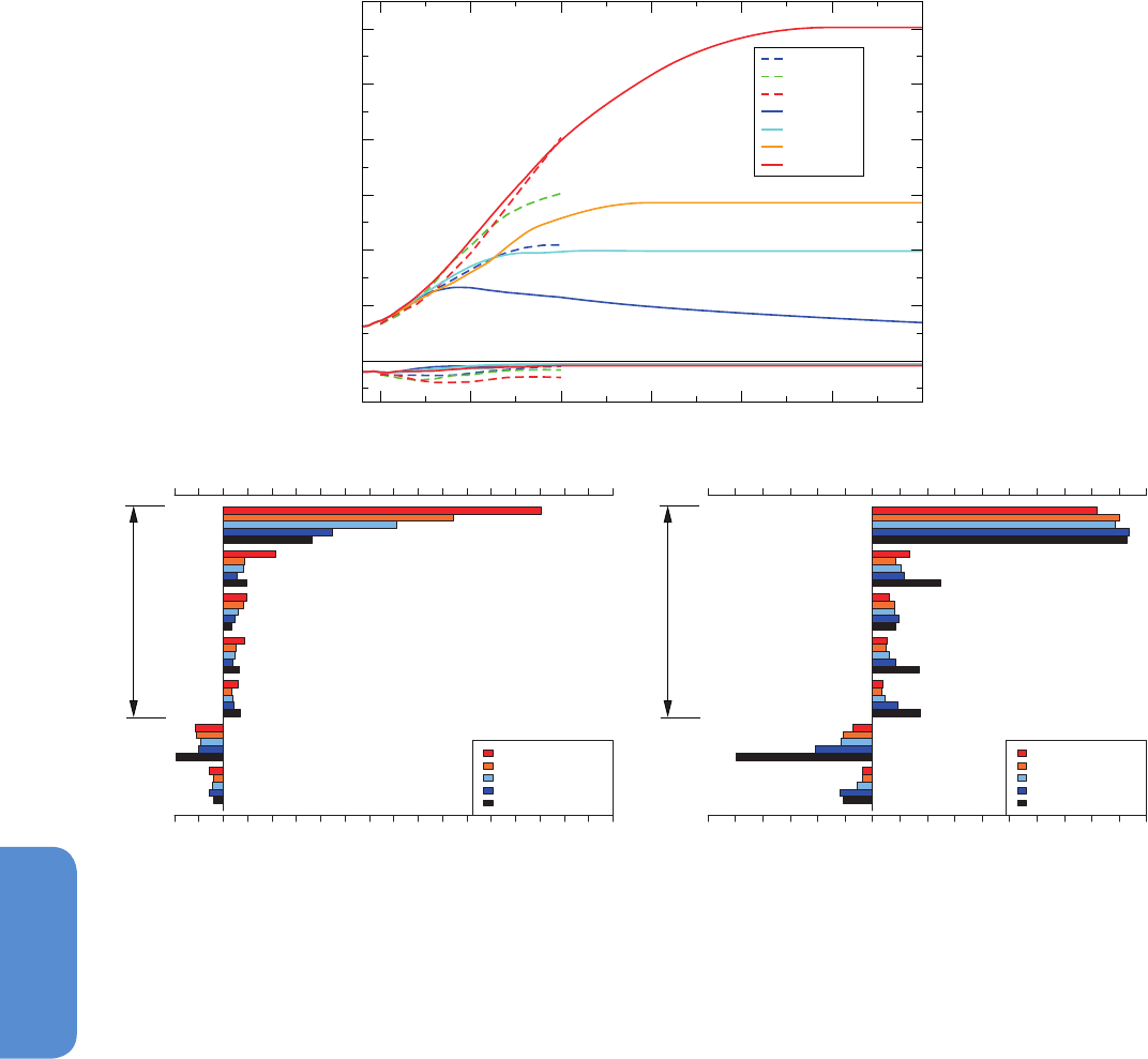
1046

Chapter 12 Long-term Climate Change: Projections, Commitments and Irreversibility

2000 2050 2100 2150220022502300

Year

Anthropogenic Radiative Forcing (W m

-2

)

SRES-B1

SRES-A1B

SRES-A2

RCP2.6

RCP4.5

RCP6.0

RCP8.5

aerosolother

OCH

RCP8.5 (2100)

RCP6.0 (2100)

RCP4.5 (2100)

RCP2.6 (2100)

present day (2010)

(W m

−2

)

Contribution of individual forcings to the total

−1.0 0.0 1.0 2.0 3.0 4.0 5.0 6.0 7.0 8.0

aerosolother

OCH

RCP8.5 (2100)

RCP6.0 (2100)

RCP4.5 (2100)

RCP2.6 (2100)

present day (2010)

(%)

Contribution of individual forcings as a percentage of the total

−60 −40 −200 20 40 60 80 100

GHG

atmospheric chemistry runs were performed to estimate ozone and

aerosol distributions (Lamarque et al., 2011). Finally, a single carbon

cycle model with a representation of carbon–climate feedbacks was

used in order to provide consistent values of CO

concentration for

the CO

emission provided by a different IAM for each of the scenari-

os. This methodology was used to produce consistent data sets across

scenarios but does not provide uncertainty estimates for them. After

these processing steps, the ﬁnal RCP data sets comprise land use

data, harmonized GHG emissions and concentrations, gridded reactive

gas and aerosol emissions, as well as ozone and aerosol abundance

ﬁelds. These data are used as forcings in individual climate models. The

number and type of forcings included primarily depend on the exper-

iment. For instance, while the CO

concentration is prescribed in most

experiments, CO

emissions are prescribed in some others (see Box 6.4

and Section 12.3.2.1). Which of these forcings are included in individ-

ual CMIP5 models, and variations in their implementation, is described

in Section 12.3.2.2.

During this development process, the total RF and the RF of individual

forcing agents have been estimated by the IAMs and made availa-

ble via the RCP database (Meinshausen et al., 2011c). Each individual

anthropogenic forcing varies from one scenario to another. They have

Figure 12.3 | (a) Time evolution of the total anthropogenic (positive) and anthropogenic aerosol (negative) radiative forcing (RF) relative to pre-industrial (about 1765) between

2000 and 2300 for RCP scenarios and their extensions (continuous lines), and SRES scenarios (dashed lines) as computed by the Integrated Assessment Models (IAMs) used to

develop those scenarios. The four RCP scenarios used in CMIP5 are: RCP2.6 (dark blue), RCP4.5 (light blue), RCP6.0 (orange) and RCP8.5 (red). The three SRES scenarios used

in CMIP3 are: B1 (blue, dashed), A1B (green, dashed) and A2 (red, dashed). Positive values correspond to the total anthropogenic RF. Negative values correspond to the forcing

from all anthropogenic aerosol–radiation interactions (i.e., direct effects only). The total RF of the SRES and RCP families of scenarios differs in 2000 because the number of forc-

ings represented and our knowledge about them have changed since the TAR. The total RF of the RCP family is computed taking into account the efﬁcacy of the various forcings

(Meinshausen et al., 2011a). (b) Contribution of the individual anthropogenic forcings to the total RF in year 2100 for the four RCP scenarios and at present day (year 2010). The

individual forcings are gathered into seven groups: carbon dioxide (CO

), methane (CH

), nitrous oxide (N

O), ozone (O

), other greenhouse gases, aerosol (all effects unlike in (a),

i.e., aerosol–radiation and aerosol–cloud interactions, aerosol deposition on snow) and land use (LU). (c) As in (b), but the individual forcings are relative to the total RF (i.e., RF

tot

, in %, with RF

individual RFs and RF

tot

total RF). Note that the RFs in (b) and (c) are not efﬁcacy adjusted, unlike in (a). The values shown in (a) are summarized in Table AII.6.8.

The values shown in (b) and (c) have been directly extracted from data ﬁles (hosted at http://tntcat.iiasa.ac.at:8787/RcpDb/) compiled by the four modelling teams that developed

the RCP scenarios and are summarized in Tables AII.6.1 to AII.6.3 for CO

, CH

and N

O respectively.

1047

Long-term Climate Change: Projections, Commitments and Irreversibility Chapter 12

been aggregated into a few groups in Figure 12.3b and c. The total

anthropogenic RF estimated by the IAMs in 2010 is about 0.15 W m

–2

lower than Chapter 8’s best estimate of ERF in 2010 (2.2 W m

–2

), the

difference arising from a revision of the RF due to aerosols and land

use in the current assessment compared to AR4. All the other individ-

ual forcings are consistent to within 0.02 W m

–2

. The change in CO

concentration is the main cause of difference in the total RF among

the scenarios (Figure 12.3b). The relative contribution

of CO

to the

total anthropogenic forcing is currently (year 2010) about 80 to 90%

and does not vary much across the scenarios (Figure 12.3c), as was

also the case for SRES scenarios (Ramaswamy et al., 2001). Aerosols

have a large negative contribution to the total forcing (about –40 to

–50% in 2010), but this contribution decreases (in both absolute and

relative terms) in the future for all the RCPs scenarios. This means that

while anthropogenic aerosols have had a cooling effect in the past,

their decrease in all RCP scenarios relative to current levels is expected

to have a net warming effect in the future (Levy II et al., 2013; see also

Figure 8.20). The 21st century decrease in the magnitude of future aer-

osol forcing was not as large and as rapid in the SRES scenarios (Figure

12.3a). However, even in the SRES scenarios, aerosol effects were

expected to have a diminishing role in the future compared to GHG

forcings, mainly because of the accumulation of GHG in the atmos-

phere (Dufresne et al., 2005). Other forcings do not change much in

the future, except CH

which increases in the RCP8.5 scenario. Note

that the estimates of all of these individual RFs are subject to many

uncertainties (see Sections 7.5, 8.5 and 11.3.6). In this section and in

Table AII.6.8, the RF values for RCP scenarios are derived from pub-

lished equivalent-CO

(CO

eq) concentration data that aggregates all

anthropogenic forcings including GHGs and aerosols. The conversion

to RF uses the formula: RF = 3.71/ln(2) ∙ ln(CO

eq/278) W m

–2

, where

eq is in ppmv.

The four RCPs (Meinshausen et al., 2011c) are based on IAMs up to the

end of the 21st century only. In order to investigate longer-term climate

change implications, these RCPs were also extended until 2300. The

extensions, formally named Extended Concentration Pathways (ECPs)

but often simply referred to as RCP extensions, use simple assump-

tions about GHG and aerosol emissions and concentrations beyond

2100 (such as stabilization or steady decline) and were designed as

hypothetical ‘what-if’ scenarios, not as an outcome of an IAM assum-

ing socioeconomic considerations beyond 2100 (Meinshausen et al.,

2011c) (see Box 1.1). In order to continue to investigate a broad range

of possible climate futures, RCP2.6 assumes small constant net nega-

tive emissions after 2100 and RCP8.5 assumes stabilization with high

emissions between 2100 and 2150, then a linear decrease until 2250.

The two middle RCPs aim for a smooth stabilization of concentrations

by 2150. RCP8.5 stabilizes concentrations only by 2250, with CO

concentrations of approximately 2000 ppmv, nearly seven times the

pre-industrial level. As RCP2.6 implies net negative CO

emissions after

around 2070 and throughout the extension, CO

concentrations slowly

reduce towards 360 ppmv by 2300.

The range of the relative contribution of CO

and aerosols to the total anthropogenic forcing is derived here from the RF values given by the IAMs and the best estimate assessed

in Chapter 8.

12.3.1.4 Comparison of Special Report on Emission Scenarios

and Representative Concentration Pathway Scenarios

The four RCP scenarios used in CMIP5 lead to RF values that range from

2.3 to 8.0 W m

–2

at 2100, a wider range than that of the three SRES

scenarios used in CMIP3 which vary from 4.2 to 8.1 W m

–2

at 2100 (see

Table AII.6.8 and Figure 12.3). The SRES scenarios do not assume any

policy to control climate change, unlike the RCP scenarios. The RF of

RCP2.6 is hence lower by 1.9 W m

–2

than the three SRES scenarios and

very close to the ENSEMBLES E1 scenario (Johns et al., 2011). RCP4.5

and SRES B1 have similar RF at 2100, and comparable time evolution

(within 0.2 W m

–2

). The RF of SRES A2 is lower than RCP8.5 through-

out the 21st century, mainly due to a faster decline in the radiative

effect of aerosols in RCP8.5 than SRES A2, but they converge to within

0.1 W m

–2

at 2100. RCP6.0 lies in between SRES B1 and SRES A1B.

Results obtained with one General Circulation Model (GCM) (Dufresne

et al., 2013) and with a reduced-complexity model (Rogelj et al., 2012)

conﬁrm that the differences in temperature responses are consistent

with the differences in RFs estimates. RCP2.6, which assumes strong

mitigation action, yields a smaller temperature increase than any SRES

scenario. The temperature increase with the RCP4.5 and SRES B1 sce-

narios are close and the temperature increase is larger with RCP8.5

than with SRES A2. The spread of projected global mean temperature

for the RCP scenarios (Section 12.4.1) is considerably larger (at both

the high and low response ends) than for the three SRES scenarios

used in CMIP3 (B1, A1B and A2) as a direct consequence of the larger

range of RF across the RCP scenarios compared to that across the

three SRES scenarios (see analysis of SRES versus RCP global tempera-

ture projections in Section 12.4.9 and Figure 12.40).

12.3.2 Implementation of Forcings in Coupled Model

Intercomparison Project Phase 5 Experiments

The CMIP5 experimental protocol for long-term transient climate

experiments prescribes a common basis for a comprehensive set of

anthropogenic forcing agents acting as boundary conditions in three

experimental phases—historical, RCPs and ECPs (Taylor et al., 2012).

To permit common implementations of this set of forcing agents in

CMIP5 models, self-consistent forcing data time series have been com-

puted and provided to participating models (see Sections 9.3.2.2 and

12.3.1.3) comprising emissions or concentrations of GHGs and related

compounds, ozone and atmospheric aerosols and their chemical pre-

cursors, and land use change.

The forcing agents implemented in Atmosphere–Ocean General Cir-

culation Models (AOGCMs) and ESMs used to make long-term cli-

mate projections in CMIP5 are summarized in Table 12.1. The number

of CMIP5 models listed here is about double the number of CMIP3

models listed in Table 10.1 of AR4 (Meehl et al., 2007b).

Natural forcings (arising from solar variability and aerosol emissions

via volcanic activity) are also speciﬁed elements in the CMIP5 exper-

imental protocol, but their future time evolutions are not prescribed

1048

Chapter 12 Long-term Climate Change: Projections, Commitments and Irreversibility

Table 12.1 | Radiative forcing agents in the CMIP5 multi-model global climate projections. See Table 9.A.1 for descriptions of the models and main model references. Earth System Models (ESMs) are highlighted in bold. Numeric superscripts

indicate model-speciﬁc references that document forcing implementations. Forcing agents are mostly implemented in close conformance with standard prescriptions (Taylor et al., 2012) and recommended data sets (Lamarque et al., 2010;

Cionni et al., 2011; Lamarque et al., 2011; Meinshausen et al., 2011c) provided for CMIP5. Variations in forcing implementations are highlighted with superscripts and expanded in the table footnotes. Entries mean: n.a.: Forcing agent is not

included in either the historical or future scenario simulations; Y: Forcing agent included (via prescribed concentrations, distributions or time series data); E: Concentrations of forcing agent calculated interactively driven by prescribed emissions

or precursor emissions; Es: Concentrations of forcing agent calculated interactively constrained by prescribed surface concentrations. For a more detailed classiﬁcation of ozone chemistry and ozone forcing implementations in CMIP5 models

see Eyring et al. (2013).

Model

Forcing Agents

Greenhouse Gases Aerosols Other

O Trop O

Strat O

CFCs SO

Black

carbon

Organic

carbon

Nitrate

Cloud

albedo

effect

Cloud

lifetime

effect

Dust Volcanic Sea salt

Land

use

Solar

ACCESS-1.0

Y Y Y

Y E E E n.a. Y Y Y

n.a. Y

ACCESS-1.3

Y Y Y

Y E E E n.a. Y Y n.a. Y

n.a. Y

BCC-CSM1.1

Y/E

Y Y Y

Y Y

n.a. n.a. n.a. Y

n.a. Y

BCC-CSM1.1(m)

Y/E

Y Y Y

Y Y

n.a. n.a. n.a. Y

n.a. Y

BNU-ESM Y/E

Y Y Y

Y Y

n.a. n.a. n.a. Y

n.a. Y

CanCM4 Y Y Y Y

Y E E E n.a. Y

n.a. Y

Y/E

st,v0

n.a. Y

CanESM2 Y/E

Y Y Y

Y E E E n.a. Y

n.a. Y

Y/E

st,v0

CCSM4

Y Y Y

Y Y

n.a. n.a. n.a. Y

Y Y

CESM1(BGC)

Y/E

Y Y Y

Y Y

n.a. n.a. n.a. Y

Y Y

CESM1(CAM5)

Y Y Y

Y E E E n.a. Y Y E Y

E Y Y

CESM1(CAM5.1,FV2)

Y Y Y

Y E E E n.a. Y Y E Y

E Y Y

CESM1(FASTCHEM) Y

Y E E Y E Y

n.a. n.a. n.a. Y

Y Y

CESM1(WACCM)

Es Es E/Es

E/Es

Es Y Y Y n.a. n.a. n.a. Y

Y Y

CMCC-CESM

Y Y Y Y

Y Y

n.a. n.a. n.a. Y

n.a. Y

CMCC-CM Y Y Y Y

Y Y

n.a. n.a. n.a. Y

n.a. Y

CMCC-CMS Y Y Y Y

Y Y

n.a. n.a. n.a. Y

n.a. Y

CNRM-CM5

Y Y Y Y

Y Y

n.a. Y

so,ic

n.a. Y

CSIRO-Mk3.6.0

Y Y Y Y

Y E E E n.a. Y Y Y

n.a. Y

EC-EARTH

Y Y Y Y

Y Y

n.a. n.a. n.a. Y

Y Y

FGOALS-g2

Y Y Y Y

Y Y

n.a. Y Y Y

n.a. Y

FGOALS-s2

Y/E Y Y Y

Y Y

n.a. n.a. n.a. Y

n.a. Y

FIO-ESM Y/E Y Y Y

Y Y

n.a. n.a. n.a. Y

n.a. Y

GFDL-CM3

Y/Es

E E Y/Es

E E E n.a./E

Y Y E

Y/E

st,v0

Y Y

GFDL-ESM2G Y/E

Y Y Y

Y Y

n.a. n.a. n.a. Y

Y Y

GFDL-ESM2M Y/E

Y Y Y

Y Y

n.a. n.a. n.a. Y

Y Y

GISS-E2-p1

Y Y Y Y

Y Y Y Y Y Y n.a. Y

Y Y

GISS-E2-p2

Y Es/E

Es E E Es/E

E E E E Y n.a. Y

Y Y

(continued on next page)

1049

Long-term Climate Change: Projections, Commitments and Irreversibility Chapter 12

Model

Forcing Agents

Greenhouse Gases Aerosols Other

O Trop O

Strat O

CFCs SO

Black

carbon

Organic

carbon

Nitrate

Cloud

albedo

effect

Cloud

lifetime

effect

Dust Volcanic Sea salt

Land

use

Solar

GISS-E2-p3

Y Es/E

Es E E Es/E

E E E E Y n.a. Y

Y Y

HadCM3 Y

Y Y Y

Y E n.a. n.a. n.a. Y

n.a. n.a. Y

HadGEM2-AO

Y Y Y

Y E E E n.a. Y Y Y

Y Y

HadGEM2-CC

16,17

Y Y Y

Y E E E n.a. Y Y Y

Y Y

HadGEM2-ES

Y/E

Es Y E Y

Y E E E n.a. Y Y Y

Y Y

INM-CM4 Y/E Y Y Y

n.a. Y

n.a. n.a. n.a. Y

n.a. n.a. Y

n.a. Y Y

IPSL-CM5A-LR

Y/E

Y Y Y

Y Y

n.a. Y n.a. Y

Y Y

IPSL-CM5A-MR

Y/E

Y Y Y

Y Y

n.a. Y n.a. Y

Y Y

IPSL-CM5B-LR

Y Y Y

Y Y

n.a. Y n.a. Y

Y Y

MIROC-ESM

Y/E

Y Y Y

Y E E E n.a. Y

Y Y

MIROC-ESM-CHEM

Y Y E E Y E E E n.a. Y

Y Y

MIROC4h

Y Y Y

Y E E E n.a. Y Y Y

MIROC5

Y Y Y

Y E E E n.a. Y

MPI-ESM-LR Y/E

Y Y Y

Y Y

n.a. n.a. Y

Y Y

MPI-ESM-MR Y

Y Y Y

Y Y

n.a. n.a. Y

Y Y

MPI-ESM-P Y

Y Y Y

Y Y

n.a. n.a. Y

Y Y

MRI-CGCM3

Y Y Y Y

Y E E E n.a. Y

Y Y

MRI-ESM1

E Y Y E E Es E E E n.a. Y

Y Y

NorESM1-M

Y Y Y

Y E E E n.a. Y Y E Y/E

st,v1

Y Y

NorESM1-ME

Y/E

Y Y Y

Y E E E n.a. Y Y E Y/E

st,v1

Y Y

Jones et al. (2011)

Hardiman et al. (2012)

Dufresne et al. (2013)

Watanabe et al. (2011)

Komuro et al. (2012)

Yukimoto et al. (2012)

Adachi et al. (2013)

Iversen et al. (2013); Kirkevåg et al. (2013); Tjiputra et al. (2013)

Notes:

Model-speciﬁc references relating to forcing implementations:

Dix et al. (2013)

Wu et al. (2013); Xin et al. (2013a, 2013b)

Meehl et al. (2012); Gent et al. (2011)

Long et al. (2013); Meehl et al. (2012)

Meehl et al. (2013)

Calvo et al. (2012); Meehl et al. (2012)

Cagnazzo et al. (2013)

Voldoire et al. (2013)

Rotstayn et al. (2012)

Hazeleger et al. (2013)

Li et al. (2013c)

Bao et al. (2013)

Levy II et al. (2013)

Shindell et al. (2013a). GISS-E2-R and GISS-E2-H model variants are forced similarly and both

represented here as GISS-E2. Both -R and -H model versions have three variants: in physics version

1 (p1) aerosols and ozone are speciﬁed from pre-computed transient aerosol and ozone ﬁelds, in

physics version 2 (p2) aerosols and atmospheric chemistry are calculated online as a function of

atmospheric state and transient emissions inventories, while in physics version 3 (p3) atmospheric

composition is calculated as for p2 but the aerosol impacts on clouds (and hence the aerosol indirect

effect) is calculated interactively. In p1 and p2 variants the aerosol indirect effect is parameterized

following Hansen et al. (2005b).

HadGEM2-AO is forced in a similar way to HadGEM2-ES and HadGEM2-CC following Jones et al.

(2011), but tropospheric ozone, stratospheric ozone and land cover are prescribed.

Table 12.1 (continued)

(continued on next page)

1050

Chapter 12 Long-term Climate Change: Projections, Commitments and Irreversibility

Additional notes:

Separate entries for CO

denote ‘concentration-driven’ and ‘emissions-driven’ experiments as indicated.

‘Cloud albedo effect’ and ‘Cloud lifetime effect’ are classical terms (as used in AR4) to describe indirect effects of radiative

forcing associated with aerosols. They relate to the revised terminologies deﬁned in Chapter 7 and used in AR5: ‘Radiative

forcing from aerosol–cloud interactions (RFaci)’ and ‘Effective radiative forcing from aerosol–cloud interactions (ERFaci)’.

RFaci equates to cloud albedo effect, while ERFaci is the effective forcing resulting from cloud albedo effect plus cloud

lifetime effect, including all rapid adjustments to cloud lifetime and thermodynamics (Section 7.1.3, Figure 7.3).

Physiological forcing effect of CO

via plant stomatal response and evapotranspiration (Betts et al., 2007) included.

Separate entries denote different treatments used for radiation and chemistry respectively.

Separate entries denote treatment for historical and future (RCPs) respectively.

Three-dimensional tropospheric ozone, stratospheric ozone, methane, and/or aerosol distributions speciﬁed as monthly

10-year mean concentrations, computed off-line using CAM-Chem – a modiﬁed version of CAM3.5 with interactive chemistry –

driven with speciﬁed emissions for the historical period (Lamarque et al., 2010) and RCPs (Lamarque et al., 2011) with sea

surface temperature and sea ice boundary conditions based on CCSM3’s projections for the closest corresponding AR4

scenarios.

Ozone prescribed using the original or slightly modiﬁed IGAC/SPARC ozone data set (Cionni et al., 2011); in some models this

data set is modiﬁed to add a future solar cycle and in some models tropospheric ozone is zonally averaged.

Linearized 2D ozone chemistry scheme (Cariolle and Teyssedre, 2007) including transport and photochemistry, reactive to

stratospheric chlorine concentrations but not tropospheric chemical emissions.

Ozone prescribed using the data set described in Hansen et al. (2007), with historical tropospheric ozone being calculated

by a CCM and stratospheric ozone taken from Randel and Wu (2007) in the past. Tropospheric ozone is held constant from

1990 onwards, while stratospheric ozone is constant from 1997 to 2003 and then returned linearly to its 1979 value over the

period 2004 to 2050.

For IPSL-CM5 model versions, ozone and aerosol concentrations are calculated semi-ofﬂine with the atmospheric general

circulation model including interactive chemistry and aerosol, following the four RCPs in the future (Dufresne et al., 2013;

Szopa et al., 2013). The same aerosol concentration ﬁelds (but not ozone) are also prescribed for the CNRM-CM5 model.

Ozone concentrations computed off-line by Kawase et al. (2011) using a CCM forced with CMIP5 emissions.

Ozone concentrations computed off-line by Sudo et al. (2003) for the historical period and Kawase et al. (2011) for the future.

Time dependent climatology based on simulations and observations; aerosols are distinguished only with respect to coarse

and ﬁne mode, and anthropogenic and natural origins, not with respect to composition.

Separate entries denote different ozone chemistry precursors.

RFaci from sulphate aerosol only.

Separate entries denote stratosphere and troposphere respectively.

Radiative effects of aerosols on ice clouds are represented.

Prognostic or diagnostic scheme for dust/sea salt aerosol with emissions/concentrations determined by the model state

rather than externally prescribed.

Fixed prescribed climatology of dust/sea salt aerosol concentrations with no year-to-year variability.

Explosive volcanic aerosol returns rapidly in future to zero (or near-zero) background, like that in the pre-industrial control

experiment.

Explosive volcanic aerosol returns rapidly in future to constant (average volcano) background, the same as in the pre-

industrial control experiment.

Explosive volcanic aerosol returns slowly in future (over several decades) to constant (average volcano) background like that

in the pre-industrial control experiment.

Explosive volcanic aerosol returns rapidly in future to near-zero background, below that in the pre-industrial control

experiment.

Explosive volcanic aerosol set to zero in future, but constant (average volcano) background in the pre-industrial control

experiment.

Explosive volcanic aerosol returns slowly in future (over several decades) to constant (average volcano) background, but zero

background in the pre-industrial control experiment.

Land use change represented via crop change only.

Realistic time-varying orbital parameters for solar forcing (in historical period only for GISS-E2).

Table 12.1 (continued)

1051

Long-term Climate Change: Projections, Commitments and Irreversibility Chapter 12

very precisely. A repeated 11-year cycle for total solar irradiance (Lean

and Rind, 2009) is suggested for future projections but the periodicity

is not speciﬁed precisely as solar cycles vary in length. Some models

include the effect of orbital variations as well, but most do not. For

volcanic eruptions, no speciﬁc CMIP5 prescription is given for future

emissions or concentration data, the general recommendation being

that volcanic aerosols should either be omitted entirely both from the

control experiment and future projections or the same background

volcanic aerosols should be prescribed in both. This provides a con-

sistent framework for model intercomparison given a lack of knowl-

edge of when future large eruptions will occur. In general models have

adhered to this guidance, but there are variations in the background

volcanic aerosol levels chosen (zero or an average volcano back-

ground in general) and some cases, for example, Australian Commu-

nity Climate and Earth System Simulator (ACCESS)1.0 and ACCESS1.3

(Dix et al., 2013), where the background volcanic aerosol in future

differs signiﬁcantly from that in the control experiment, with a small

effect on future RF.

For the other natural aerosols (dust, sea-salt, etc.), no emission or

concentration data are recommended. The emissions are potentially

computed interactively by the models themselves and may change

with climate, or prescribed from separate model simulations carried

out in the implementation of CMIP5 experiments, or simply held con-

stant. Natural aerosols (mineral dust and sea salt) are in a few cases

prescribed with no year-to-year variation (giving no transient forcing

effect), in some cases prescribed from data sets computed off-line as

described above, and in other cases calculated interactively via prog-

nostic or diagnostic calculations. The degree to which natural aerosol

emissions are interactive is effectively greater in some such models

than others, however, as mineral dust emissions are more constrained

when land vegetation cover is speciﬁed (e.g., as in Commonwealth

Scientiﬁc and Industrial Research Organisation (CSIRO)-Mk3.6.0) (Rot-

stayn et al., 2012) than when vegetation is allowed to evolve dynami-

cally (e.g., as in Hadley Centre new Global Environmental Model 2-ES

(HadGEM2-ES)) (Jones et al., 2011) (Table 9.A.1).

12.3.2.1 ‘Emissions-Driven’ versus ‘Concentration Driven’

Experiments

A novel feature within the CMIP5 experimental design is that experi-

ments with prescribed anthropogenic emissions are included in addi-

tion to classical experiments with prescribed concentration pathways

for WMGHGs (Taylor et al., 2012). The essential features of these two

classes of experiment are described in Box 6.4. The CMIP5 protocol

includes experiments in which ‘ESMs’ (models possessing at least a

carbon cycle, allowing for interactive calculation of atmospheric CO

or compatible emissions) and AOGCMs (that do not possess such an

interactive carbon cycle) are both forced with WMGHG concentration

pathways to derive a range of climate responses consistent with those

pathways from the two types of model. The range of climate responses

including climate–carbon cycle feedbacks can additionally be explored

in ESMs driven with emissions rather than concentrations, analogous

to Coupled Climate Carbon Cycle Model Intercomparison Project

MIP) experiments (Friedlingstein et al., 2006)—see Box 6.4. Results

from the two types of experiment cannot be compared directly, but

they provide complementary information. Uncertainties in the forward

climate response driven with speciﬁed emissions or concentrations can

be derived from all participating models, while concentration-driven

ESM experiments also permit a policy-relevant diagnosis of the range

of anthropogenic carbon emissions compatible with the imposed con-

centration pathways (Hibbard et al., 2007; Moss et al., 2010).

WMGHG forcing implementations in CMIP5 concentration-driven

experiments conform closely in almost all cases to the standard proto-

col (Table 12.1; CO

, CH

, N

O, chloroﬂuorocarbons (CFCs)), imposing

an effective control over the RF due to WMGHGs across the multi-mod-

el ensemble, apart from the model spread arising from radiative trans-

fer codes (Collins et al., 2006b; Meehl et al., 2007b). The ability of ESMs

to determine their own WMGHG concentrations in emissions-driven

experiments means that RF due to WMGHGs is less tightly controlled

in such experiments. Even in concentration-driven experiments, many

models implement some emissions-driven forcing agents (more often

aerosols, but also ozone in some cases), leading to a potentially great-

er spread in both the concentrations and hence RF of those emis-

sions-driven agents.

12.3.2.2 Variations Between Model Forcing Implementations

Apart from the distinction between concentration-driven and emis-

sions-driven protocols, a number of variations are present in the imple-

mentation of forcing agents listed in Table 12.1, which generally arise

due to constraining characteristics of the model formulations, various

computational efﬁciency considerations or local implementation deci-

sions. In a number of models, off-line modelling using an aerosol chem-

istry climate model has been used to convert emissions into concentra-

tions compatible with the speciﬁc model formulation or characteristics.

As a result, although detailed prescriptions are given for the forcing

agents in CMIP5 experiments in emissions terms, individual modelling

approaches lead to considerable variations in their implementations

and consequential RFs. This was also the case in the ENSEMBLES mul-

ti-model projections, in which similar forcing agents to CMIP5 models

were applied but again with variations in the implementation of aer-

osol, ozone and land use forcings, prescribing the SRES A1B and E1

scenarios in a concentration-driven protocol (Johns et al., 2011) akin

to the CMIP5 protocol.

Methane, nitrous oxide and CFCs (typically with some aggregation of

the multiple gases) are generally prescribed in CMIP5 models as well-

mixed concentrations following the forcing data time series provid-

ed for the given scenarios. In a number of models (CESM1(WACCM),

GFDL-CM3, GISS-E2-p2, GISS-E2-p3, HadGEM2-ES and MRI-ESM1) the

three-dimensional concentrations in the atmosphere of some species

evolve interactively driven by the full emissions/sinks cycle (in some

cases constrained by prescribed concentrations at the surface, e.g.,

HadGEM2-ES for methane). In cases where the full emissions/sinks

cycle is modelled, the radiation scheme is usually passed the time-var-

ying 3-D concentrations, but some models prescribe different concen-

trations for the purpose of radiation.

Eyring et al. (2013) document, in greater detail than Table 12.1, the

implementations of tropospheric and stratospheric ozone in CMIP5

models, including their ozone chemistry schemes and modiﬁcations

applied to reference data sets in models driven by concentrations. In

1052

Chapter 12 Long-term Climate Change: Projections, Commitments and Irreversibility

most models that prescribe ozone, concentrations are based on the

original or slightly modiﬁed CMIP5 standard ozone data set comput-

ed as part of the International Global Atmospheric Chemistry/Strat-

ospheric Processes and their Role in Climate (IGAC/SPARC) activity

(Cionni et al., 2011). In the stratosphere, this data set is based on

observations of the past (Randel and Wu, 2007) continued into the

future with the multi-model mean of 13 chemistry–climate models

(CCMs) projections following the SRES A1B (IPCC, 2000) and SRES

A1 adjusted halogen scenario (WMO, 2007). The stratospheric zonal

mean ozone ﬁeld is merged with a 3-D tropospheric ozone time series

generated as the mean of two CCMs (Goddard Institute of Space

Studies-Physical Understanding of Composition-Climate Interactions

and Impacts (GISS-PUCCINI), Shindell et al., 2006; CAM3.5, Lamarque

et al., 2010) in the past and continued by one CCM (CAM3.5) in the

future. Some CMIP5 models (MIROC-ESM, MIROC4h, MIROC5 and

GISS-E2-p1) prescribe ozone concentrations using different data sets

but again following just one GHG scenario in the future for the projec-

tion of stratospheric ozone. In other models (e.g., Institut Pierre Simon

Laplace (IPSL)-CM5, CCSM4) ozone is again prescribed, but supplied as

concentrations from off-line computations using a related CCM. Some

models determine ozone interactively from speciﬁed emissions via

on-line atmospheric chemistry (CESM1(FASTCHEM), CESM1(WACCM),

CNRM-CM5, GFDL-CM3, GISS-E2-p2, GISS-E2-p3, MIROC-ESM-CHEM,

MRI-ESM1; and HadGEM2-ES for tropospheric ozone only). Computing

ozone concentrations interactively allows the fast coupling between

chemistry and climate to be captured, but modelling of chemistry pro-

cesses is sometimes simpliﬁed (CNRM-CM5, CESM(FASTCHEM)) in

comparison with full complexity CCMs to reduce the computational

cost. Compared to CMIP3, in which all models prescribed ozone and

around half of them used a ﬁxed ozone climatology, this leads to sub-

stantial improvement to ozone forcings in CMIP5, although differences

remain among the models with interactive chemistry.

For atmospheric aerosols, either aerosol precursor emissions-driven

or concentration-driven forcings are applied depending on individu-

al model characteristics (see Sections 7.3 and 7.4 for an assessment

of aerosols processes including aerosol–radiation and aerosol–cloud

interactions). A larger fraction of models in CMIP5 than CMIP3 pre-

scribe aerosol precursor emissions rather than concentrations. Many

still prescribe concentrations pre-computed either using a directly relat-

ed aerosol CCM or from output of another, complex, emissions-driven

aerosol chemistry model within the CMIP5 process. As for ozone, aer-

osol concentrations provided from off-line simulations help to reduce

the computational burden of the projections themselves. For several

of the concentration-driven models (CCSM4, IPSL-CM5A variants,

MPI-ESM-LR, MPI-ESM-MR), additional emissions-driven simulations

have been undertaken to tailor the prescribed concentrations closely

to the model’s individual aerosol–climate characteristics. Lamarque et

al. (2010, 2011) provided the recommended CMIP5 aerosols data set

which has been used in several of the models driven by concentrations.

Compared with the CMIP3 models, a much larger fraction of CMIP5

models now incorporate black and organic carbon aerosol forcings.

Also, a larger fraction of CMIP5 than CMIP3 models now includes a

range of processes that combine in the effective RF from aerosol–

cloud interactions (ERFaci; see Section 7.1.3 and Figure 7.3). Previ-

ously such processes were generally termed aerosol indirect effects,

usually separated into cloud albedo (or ﬁrst indirect) effect and cloud

lifetime (or second indirect) effect. Many CMIP5 models only include

the interaction between sulphate aerosol and cloud, and the majority

of them only model the effect of aerosols on cloud albedo rather than

cloud lifetime (Table 12.1). No CMIP5 models represent urban aero-

sol pollution explicitly so that is not listed in Table 12.1 (see Section

11.3.5.2 for discussion of future air quality). Only one model (GISS-E2)

explicitly includes nitrate aerosol as a separate forcing, though it is

also included within the total aerosol mixture in the Max Planck Insti-

tute-Earth System Model (MPI-ESM) model versions.

Land use change is typically applied by blending anthropogenic land

surface disturbance via crop and pasture fraction changes with under-

lying land cover maps of natural vegetation, but model variations

in the underlying land cover maps and biome modelling mean that

the land use forcing agent is impossible to impose in a completely

common way at present (Pitman et al., 2009). Most CMIP5 models rep-

resent crop and pasture disturbance separately, while some (Canadian

Earth System Model (CanESM2), MIROC4h, MIROC5) represent crop

but not pasture. Some models (e.g., HadGEM2-ES, MIROC-ESM and

MPI-ESM versions) allow a dynamical representation of natural vege-

tation changes alongside anthropogenic disturbance (see also Sections

9.4.4.3 and 9.4.4.4).

Treatment of the CO

emissions associated with land cover chang-

es is also model dependent. Some models do not account for land

cover changes at all, some simulate the biophysical effects but are

still forced externally by land cover change induced CO

emissions (in

emissions-driven simulations), while the most advanced ESMs simu-

late both biophysical effects of land cover changes and their associ-

ated CO

emissions.

12.3.3 Synthesis of Projected Global Mean Radiative

Forcing for the 21st Century

Quantiﬁcation of future global mean RF is of interest as it is directly

related to changes in the global energy balance of the climate system

and resultant climate change. Chapter 8 discusses RF concepts and

methods for computing it that form the basis of analysis directly from

the output of model projections.

We assess three related estimates of projected global mean forc-

ing and its range through the 21st century in the context of forcing

estimated for the recent past (Figure 12.4). The estimates used are:

the total forcings for the deﬁned RCP scenarios, harmonized to RF in

the past (Meinshausen et al., 2011a; Meinshausen et al., 2011c); the

total effective radiative forcing (ERF) estimated from CMIP5 models

through the 21st century for the four RCP experiments (Forster et al.,

2013); and that estimated from models in the Atmospheric Chemistry

and Climate Model Intercomparison Project (ACCMIP; Lamarque et

al., 2013—see Section 8.2.2 ) for RCP time-slice experiments (Shindell

et al., 2013b). Methodological differences mean that whereas CMIP5

estimates include both natural and anthropogenic forcings based

entirely on ERF, ACCMIP estimates anthropogenic composition forcing

only (neglecting forcing changes due to natural, i.e., solar and volca-

nic, and land use factors) based on a combination of ERF for aerosols

and RF for WMGHG (see Section 8.5.3). Note also that total forcing

for the deﬁned RCP scenarios is based on Meinshausen et al. (2011c)

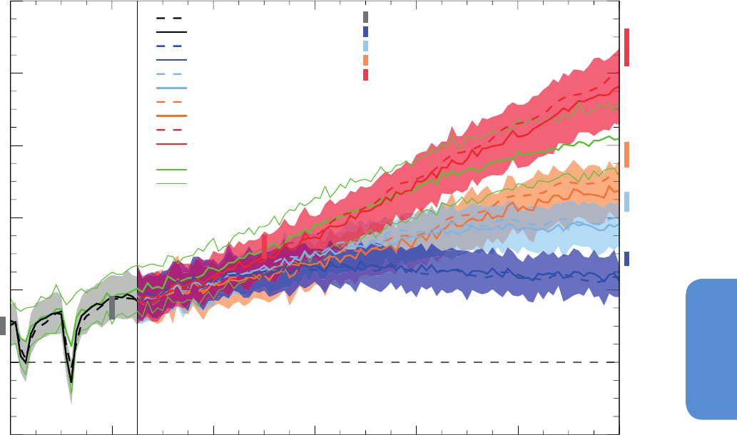
1053

Long-term Climate Change: Projections, Commitments and Irreversibility Chapter 12

1980 2000 2020 2040 2060 2080 2100

Year

-2

Radiative Forcing (W m

-2

)

historical

historical (CMIP5)

RCP2.6

RCP2.6 (CMIP5)

RCP4.5

RCP4.5 (CMIP5)

RCP6.0

RCP6.0 (CMIP5)

RCP8.5

RCP8.5 (CMIP5)

historical (ACCMIP)

RCP2.6 (ACCMIP)

RCP4.5 (ACCMIP)

RCP6.0 (ACCMIP)

RCP8.5 (ACCMIP)

20C3M+A1B (CMIP3)

+/- 1 Stdev

but combining total anthropogenic ERF (allowing for efﬁcacies of the

various anthropogenic forcings as in Figure 12.3) with natural (solar

and volcanic) RF.

The CMIP5 multi-model ensemble mean ERF at 2100 (relative to an

1850–1869 base period) is 2.2, 3.8, 4.8 and 7.6 W m

–2

respectively for

RCP2.6, RCP4.5, RCP6.0 and RCP8.5 concentration-driven projections,

with a 1-σ range based on annual mean data for year 2100 of about

±0.5 to 1.0 W m

–2

depending on scenario (lowest for RCP2.6 and high-

est for RCP8.5). The CMIP5-based ERF estimates are close to the total

forcing at 2100 (relative to an 1850–1859 base period) of 2.4, 4.0, 5.2

and 8.0 W m

–2

as deﬁned for the four RCPs.

The spread in ERF indicated from CMIP5 model results with speciﬁed

GHG concentration pathways is broadly consistent with that found for

Figure 12.4 | Global mean radiative forcing (RF, W m

–2

) between 1980 and 2100 estimated by alternative methods. The baseline is circa 1850 but dependent on the methods.

Dashed lines indicate the total anthropogenic plus natural (solar and volcanic) RF for the RCP scenarios as deﬁned by Meinshausen et al. (2011c), taking into account the efﬁcacies

of the various anthropogenic forcings (Meinshausen et al., 2011a), normalized by the mean between 1850 and 1859. Solid lines are multi-model mean effective radiative forcing

(ERF) realized in a subset of CMIP5 models for the concentration-driven historical experiment and RCP scenarios, normalized either with respect to the 1850–1869 base period

or with respect to the pre-industrial control simulation (Forster et al., 2013). (The subset of CMIP5 models included is deﬁned by Table 1 of Forster et al. (2013) but omitting the

FGOALS-s2 (Flexible Global Ocean-Atmosphere-Land System) model, the historical and RCP simulations of which were subsequently withdrawn from the CMIP5 archive.) This

CMIP5-based estimate assumes each model has an invariant climate feedback parameter, calculated from abrupt 4 × CO

experiments using the method of Gregory et al. (2004).

Each individual CMIP5 model’s forcing estimate is an average over all available ensemble members, and a 1-σ inter-model range around the multi-model mean is shaded in light

colour. Grey or coloured vertical bars illustrate the 1-σ range (68% conﬁdence interval) of anthropogenic composition forcing (excluding natural and land use change forcings,

based on ERF for aerosols combined with RF for WMGHG) estimated in ACCMIP models (Shindell et al., 2013b) for time slice experiments at 1980, 2000, 2030 (RCP8.5 only) and

2100 (all RCPs). The ACCMIP ranges plotted have been converted from the 5 to 95% ranges given in Shindell et al. (2013b) (Table 8) to a 1-σ range. Note that the ACCMIP bars at

1980 and 2100 are shifted slightly to aid clarity. The mean ERF diagnosed from 21 CMIP3 models for the SRES A1B scenario, as in Forster and Taylor (2006), is also shown (thick

green line) with a 1-σ range (thinner green lines). The number of models included in CMIP3 and CMIP5 ensemble means is shown colour coded. (See Tables AII.6.8 to AII.6.10.

Note that the CMIP5 model ranges given in Table AII.6.10 are based on decadal averages and therefore differ slightly from the ranges based on annual data shown in this ﬁgure.)

CMIP3 models for the A1B scenario using the corresponding method

(Forster and Taylor, 2006). As for CMIP3 models, part of the forcing

spread in CMIP5 models (Forster et al., 2013) is consistent with differ-

ences in GHG forcings arising from the radiative transfer codes (Col-

lins et al., 2006b). Aerosol forcing implementations in CMIP5 models

also vary considerably, however (Section 12.3.2), leading to a spread

in aerosol concentrations and forcings which contributes to the overall

model spread. A further small source of spread in CMIP5 results pos-

sibly arises from an underlying ambiguity in the CMIP5 experimental

design regarding the volcanic forcing offset between the historical

experiment versus the pre-industrial control experiment. Most models

implement zero volcanic forcing in the control experiment but some

use constant negative forcing equal to the time-mean of historical

volcanic forcing (see Table 12.1 and Section 12.3.2). The effect of this

volcanic forcing offset persists into the future projections.

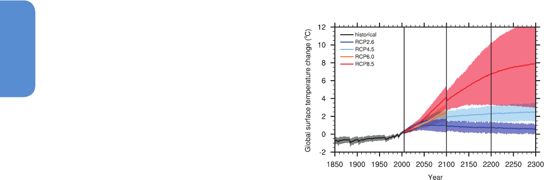
1054

Chapter 12 Long-term Climate Change: Projections, Commitments and Irreversibility

ACCMIP projected forcing at 2030 (for RCP8.5) and 2100 (all RCPs) is

systematically higher than corresponding CMIP5 ERF, although with

some overlap between 1-σ ranges. CMIP5 and ACCMIP comprise dif-

ferent sets of models and they are related in many but not all cases

(Section 8.2.2). Conﬁning analysis to a subset of closely related models

also gives higher forcing estimates from ACCMIP compared to CMIP5

so the discrepancy in multi-model ensemble mean forcings appears

unrelated to the different model samples associated with the two

methods of estimation. The discrepancy is thought to originate mostly

from differences in the underlying methodologies used to estimate RF,

but is not yet well understood (see also Section 8.5.3).

There is high conﬁdence in projections from ACCMIP models (Shindell

et al., 2013b) based on the GISS-E2 CMIP5 simulations (Shindell et al.,

2013a) and an earlier study with a version of the HadGEM2-ES model

related to that used in CMIP5 (Bellouin et al., 2011), consistent with

understanding of the processes controlling nitrate formation (Adams

et al., 2001), that nitrate aerosols (which provide a negative forcing)

will increase substantially over the 21st century under the RCPs (Sec-

tion 8.5.3, Figure 8.20). The magnitude of total aerosol-related forcing

(also negative in sign) will therefore tend to be underestimated in the

CMIP5 multi-model mean ERF, as nitrate aerosol has been omitted as a

forcing from almost all CMIP5 models.

Natural RF variations are, by their nature, difﬁcult to project reliably

(see Section 8.4). There is very high conﬁdence that Industrial Era nat-

ural forcing has been a small fraction of the (positive) anthropogenic

forcing except for brief periods following large volcanic eruptions (Sec-

tions 8.5.1 and 8.5.2). Based on that assessment and the assumption

that variability in natural forcing remains of a similar magnitude and

character to that over the Industrial Era, total anthropogenic forcing

relative to pre-industrial, for any of the RCP scenarios through the 21st

century, is very likely to be greater in magnitude than changes in natu-

ral (solar plus volcanic) forcing on decadal time scales.

In summary, global mean forcing projections derived from climate

models exhibit a substantial range for the given RCP scenarios in con-

centration-driven experiments, contributing to the projected global

mean temperature range (Section 12.4.1). Forcings derived from

ACCMIP models for 2100 are systematically higher than those estimat-

ed from CMIP5 models for reasons that are not fully understood but

are partly due to methodological differences. The multi-model mean

estimate of combined anthropogenic plus natural forcing from CMIP5

is consistent with indicative RCP forcing values at 2100 to within 0.2

to 0.4 W m

–2

12.4 Projected Climate Change over the

21st Century

12.4.1 Time-Evolving Global Quantities

12.4.1.1 Projected Changes in Global Mean Temperature and

Precipitation

A consistent and robust feature across climate models is a continua-

tion of global warming in the 21st century for all the RCP scenarios

(Figure 12.5 showing changes in concentration-driven model simu-

lations). Temperature increases are almost the same for all the RCP

scenarios during the ﬁrst two decades after 2005 (see Figure 11.25).

At longer time scales, the warming rate begins to depend more on

the speciﬁed GHG concentration pathway, being highest (>0.3°C per

decade) in the highest RCP8.5 and signiﬁcantly lower in RCP2.6, par-

ticularly after about 2050 when global surface temperature response

stabilizes (and declines thereafter). The dependence of global temper-

ature rise on GHG forcing at longer time scales has been conﬁrmed by

several studies (Meehl et al., 2007b). In the CMIP5 ensemble mean,

global warming under RCP2.6 stays below 2°C above 1850-1900

levels throughout the 21st century, clearly demonstrating the potential

of mitigation policies (note that to translate the anomalies in Figure

12.5 into anomalies with respect to that period, an assumed 0.61°C

of observed warming since 1850–1900, as discussed in Section 2.4.3,

should be added). This is in agreement with previous studies of aggres-

sive mitigation scenarios (Johns et al., 2011; Meehl et al., 2012). Note,

however, that some individual ensemble members do show warming

exceeding 2°C above 1850-1900 (see Table 12.3). As for the other

pathways, global warming exceeds 2°C within the 21st century under

RCP4.5, RCP6.0 and RCP8.5, in qualitative agreement with previous

studies using the SRES A1B and A2 scenarios (Joshi et al., 2011). Global

mean temperature increase exceeds 4°C under RCP8.5 by 2100. The

CMIP5 concentration-driven global temperature projections are broad-

ly similar to CMIP3 SRES scenarios discussed in AR4 (Meehl et al.,

2007b) and Section 12.4.9, although the overall range of the former

is larger primarily because of the low-emission mitigation pathway

RCP2.6 (Knutti and Sedláček, 2013).

The multi-model global mean temperature changes under different

RCPs are summarized in Table 12.2. The relationship between cumu-

lative anthropogenic carbon emissions and global temperature is

assessed in Section 12.5 and only concentration-driven models are

42 models

Figure 12.5 | Time series of global annual mean surface air temperature anomalies

(relative to 1986–2005) from CMIP5 concentration-driven experiments. Projections are

shown for each RCP for the multi-model mean (solid lines) and the 5 to 95% range

(±1.64 standard deviation) across the distribution of individual models (shading). Dis-

continuities at 2100 are due to different numbers of models performing the exten-

sion runs beyond the 21st century and have no physical meaning. Only one ensemble

member is used from each model and numbers in the ﬁgure indicate the number of

different models contributing to the different time periods. No ranges are given for the

RCP6.0 projections beyond 2100 as only two models are available.

1055

Long-term Climate Change: Projections, Commitments and Irreversibility Chapter 12

RCP2.6 (ΔT in °C) RCP4.5 (ΔT in °C) RCP6.0 (ΔT in °C) RCP8.5 (ΔT in °C)

Global: 2046–2065 1.0 ± 0.3 (0.4, 1.6) 1.4 ± 0.3 (0.9, 2.0) 1.3 ± 0.3 (0.8, 1.8) 2.0 ± 0.4 (1.4, 2.6)

2081–2100 1.0 ± 0.4 (0.3, 1.7) 1.8 ± 0.5 (1.1, 2.6) 2.2 ± 0.5 (1.4, 3.1) 3.7 ± 0.7 (2.6, 4.8)

2181–2200 0.7 ± 0.4 (0.1, 1.3) 2.3 ± 0.5 (1.4, 3.1) 3.7 ± 0.7 (-,-) 6.5 ± 2.0 (3.3, 9.8)

2281–2300 0.6 ± 0.3 (0.0, 1.2) 2.5 ± 0.6 (1.5, 3.5) 4.2 ± 1.0 (-,-) 7.8 ± 2.9 (3.0, 12.6)

Land: 2081–2100 1.2 ± 0.6 (0.3, 2.2) 2.4 ± 0.6 (1.3, 3.4) 3.0 ± 0.7 (1.8, 4.1) 4.8 ± 0.9 (3.4, 6.2)

Ocean: 2081–2100 0.8 ± 0.4 (0.2, 1.4) 1.5 ± 0.4 (0.9, 2.2) 1.9 ± 0.4 (1.1, 2.6) 3.1 ± 0.6 (2.1, 4.0)

Tropics: 2081–2100 0.9 ± 0.3 (0.3, 1.4) 1.6 ± 0.4 (0.9, 2.3) 2.0 ± 0.4 (1.3, 2.7) 3.3 ± 0.6 (2.2, 4.4)

Polar: Arctic: 2081–2100 2.2 ± 1.7 (-0.5, 5.0) 4.2 ± 1.6 (1.6, 6.9) 5.2 ± 1.9 (2.1, 8.3) 8.3 ± 1.9 (5.2, 11.4)

Polar: Antarctic: 2081–2100 0.8 ± 0.6 (-0.2, 1.8) 1.5 ± 0.7 (0.3, 2.7) 1.7 ± 0.9 (0.2, 3.2) 3.1 ± 1.2 (1.1, 5.1)

included here. Warming in 2046–2065 is slightly larger under RCP4.5

compared to RCP6.0, consistent with its greater total anthropogenic

forcing at that time (see Table A.II.6.12). For all other periods the mag-

nitude of global temperature change increases from RCP2.6 to RCP8.5.

Beyond 2100, RCP2.6 shows a decreasing trend whereas under all

other RCPs warming continues to increase. Also shown in Table 12.2

are projected changes at 2081–2100 averaged over land and ocean

separately as well as area-weighted averages over the Tropics (30°S

to 30°N), Arctic (67.5°N to 90°N) and Antarctic (90°S to 55°S) regions.

Surface air temperatures over land warm more than over the ocean,

and northern polar regions warm more than the tropics. The excess of

land mass in the Northern Hemisphere (NH) in comparison with the

Southern Hemisphere (SH), coupled with the greater uptake of heat by

the Southern Ocean in comparison with northern ocean basins means

that the NH generally warms more than the SH. Arctic warming is much

greater than in the Antarctic, due to the presence of the Antarctic ice

sheet and differences in local responses in snow and ice. Mechanisms

behind these features of warming are discussed in Section 12.4.3.

Maps and time series of regional temperature changes are displayed in

Annex I and regional averages are discussed in Section 14.8.1.

Global annual multi-model mean temperature changes above 1850-

1900 are listed in Table 12.3 for the 2081–2100 period (assuming

0.61°C warming since 1850–1900 as discussed in Section 2.4.3)

along with the percentage of 2081–2100 projections from the CMIP5

models exceeding policy-relevant temperature levels under each RCP.

These complement a similar discussion for the near-term projections

in Table 11.3 which are based on the CMIP5 ensemble as well as

evidence (discussed in Sections 10.3.1, 11.3.2.1.1 and 11.3.6.3) that

some CMIP5 models have a higher sensitivity to GHGs and a larger

response to other anthropogenic forcings (dominated by the effects

of aerosols) than the real world (medium conﬁdence). The percent-

age calculations for the long-term projections in Table 12.3 are based

solely on the CMIP5 ensemble, using one ensemble member for each

model. For these long-term projections, the 5 to 95% ranges of the

CMIP5 model ensemble are considered the likely range, an assess-

ment based on the fact that the 5 to 95% range of CMIP5 models’

TCR coincides with the assessed likely range of the TCR (see Section

12.4.1.2 below and Box 12.2). Based on this assessment, global mean

temperatures averaged in the period 2081–2100 are projected to

likely exceed 1.5°C above 1850-1900 for RCP4.5, RCP6.0 and RCP8.5

(high conﬁdence). They are also likely to exceed 2°C above 1850-1900

for RCP6.0 and RCP8.5 (high conﬁdence) and more likely than not

to exceed 2°C for RCP4.5 (medium conﬁdence). Temperature change

above 2°C under RCP2.6 is unlikely but is assessed only with medium

conﬁdence as some CMIP5 ensemble members do produce a global

mean temperature change above 2°C. Warming above 4°C by 2081–

2100 is unlikely in all RCPs (high conﬁdence) except RCP8.5. Under

the latter, the 4°C global temperature level is exceeded in more than

half of ensemble members, and is assessed to be about as likely as not

(medium conﬁdence). Note that the likelihoods of exceeding speciﬁc

temperature levels show some sensitivity to the choice of reference

period (see Section 11.3.6.3).

CMIP5 models on average project a gradual increase in global precip-

itation over the 21st century: change exceeds 0.05 mm day

–1

(~2%

of global precipitation) and 0.15 mm day

–1

(~5% of global precipi-

tation) by 2100 in RCP2.6 and RCP8.5, respectively. The relationship

between global precipitation and global temperature is approximately

linear (Figure 12.6). The precipitation sensitivity, that is, the change of

global precipitation with temperature, is about 1 to 3% °C

–1

in most

models, tending to be highest for RCP2.6 and RCP4.5 (Figure 12.7;

note that only global values are discussed in this section, ocean and

land changes are discussed in Section 12.4.5.2). These behaviours are

consistent with previous studies, including CMIP3 model projections

for SRES scenarios and AR4 constant composition commitment exper-

iments (Meehl et al., 2007b), and ENSEMBLES multi-model results for

SRES A1B and E1 scenarios (Johns et al., 2011).

The processes that govern global precipitation changes are now well

understood and have been presented in Section 7.6. They are brieﬂy

summarized here and used to interpret the long-term projected chang-

es. The precipitation sensitivity (about 1 to 3% °C

–1

) is very different

from the water vapour sensitivity (~7% °C

–1

) as the main physical

Table 12.2 | CMIP5 annual mean surface air temperature anomalies (°C) from the 1986–2005 reference period for selected time periods, regions and RCPs. The multi-model

mean ±1 standard deviation ranges across the individual models are listed and the 5 to 95% ranges from the models’ distribution (based on a Gaussian assumption and obtained

by multiplying the CMIP5 ensemble standard deviation by 1.64) are given in brackets. Only one ensemble member is used from each model and the number of models differs for

each RCP (see Figure 12.5) and becomes signiﬁcantly smaller after 2100. No ranges are given for the RCP6.0 projections beyond 2100 as only two models are available. Using

Hadley Centre/Climate Research Unit gridded surface temperature data set 4 (HadCRUT4) and its uncertainty estimate (5 to 95% conﬁdence interval), the observed warming to the

1986–2005 reference period (see Section 2.4.3) is 0.61°C ± 0.06°C (1850–1900), 0.30°C ± 0.03°C (1961–1990), 0.11°C ± 0.02°C (1980–1999). Decadal values are provided

in Table AII.7.5, but note that percentiles of the CMIP5 distributions cannot directly be interpreted in terms of calibrated language.

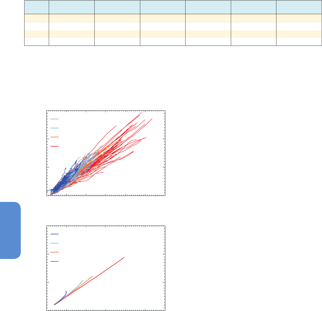
1056

Chapter 12 Long-term Climate Change: Projections, Commitments and Irreversibility

Table 12.3 | CMIP5 global annual mean temperature changes above 1850-1900 for the 2081–2100 period of each RCP scenario (mean, ±1 standard deviation and 5 to 95%

ranges based on a Gaussian assumption and obtained by multiplying the CMIP5 ensemble standard deviation by 1.64), assuming 0.61°C warming has occurred prior to 1986–2005

(second column). For a number of temperature levels (1°C, 1.5°C, 2°C, 3°C and 4°C), the proportion of CMIP5 model projections for 2081–2100 above those levels under each

RCP scenario are listed. Only one ensemble member is used for each model.

laws that drive these changes also differ. Water vapour increases are

primarily a consequence of the Clausius–Clapeyron relationship asso-

ciated with increasing temperatures in the lower troposphere (where

most atmospheric water vapour resides). In contrast, future precipi-

tation changes are primarily the result of changes in the energy bal-

ance of the atmosphere and the way that these later interact with

Figure 12.6 | Global mean precipitation (mm day

–1

) versus temperature (°C) changes

relative to 1986–2005 baseline period in CMIP5 model concentrations-driven projec-

tions for the four RCPs for (a) means over decadal periods starting in 2006 and over-

lapped by 5 years (2006–2015, 2011–2020, up to 2091–2100), each line representing

a different model (one ensemble member per model) and (b) corresponding multi-model

means for each RCP.

0 1 2 3 4 5 6

Temperature change (°C)

0.0

0.1

0.2

0.3

Precipitation change (mm day

-1

)

RCP2.6

RCP4.5

RCP6.0

RCP8.5

0 1 2 3 4 5 6

Temperature change (°C)

0.0

0.1

0.2

0.3

Precipitation change (mm day

-1

)

RCP2.6

RCP4.5

RCP6.0

RCP8.5

∆T (°C)

2081–2100

∆T > +1.0°C ∆T > +1.5°C ∆T > +2.0°C ∆T > +3.0°C ∆T > +4.0°C

RCP2.6 1.6 ± 0.4 (0.9, 2.3) 94% 56% 22% 0% 0%

RCP4.5 2.4 ± 0.5 (1.7, 3.2) 100% 100% 79% 12% 0%

RCP6.0 2.8 ± 0.5 (2.0, 3.7) 100% 100% 100% 36% 0%

RCP8.5 4.3 ± 0.7 (3.2, 5.4) 100% 100% 100% 100% 62%

circulation, moisture and temperature (Mitchell et al., 1987; Boer, 1993;

Vecchi and Soden, 2007; Previdi, 2010; O’Gorman et al., 2012). Indeed,

the radiative cooling of the atmosphere is balanced by latent heat-

ing (associated with precipitation) and sensible heating. Since AR4,

the changes in heat balance and their effects on precipitation have

been analyzed in detail for a large variety of forcings, simulations and

models (Takahashi, 2009a; Andrews et al., 2010; Bala et al., 2010; Ming

et al., 2010; O’Gorman et al., 2012; Bony et al., 2013).

An increase of CO

decreases the radiative cooling of the troposphere

and reduces precipitation (Andrews et al., 2010; Bala et al., 2010). On

longer time scales than the fast hydrological adjustment time scale

(Andrews et al., 2010; Bala et al., 2010; Cao et al., 2012; Bony et al.,

2013), the increase of CO

induces a slow increase of temperature and

water vapour, thereby enhancing the radiative cooling of the atmos-

phere and increasing global precipitation (Allen and Ingram, 2002;

Yang et al., 2003; Held and Soden, 2006). Even after the CO

forcing

stabilizes or begins to decrease, the ocean continues to warm, which

then drives up global temperature, evaporation and precipitation. In

addition, nonlinear effects also affect precipitation changes (Good et

al., 2012). These different effects explain the steepening of the precip-

itation versus temperature relationship in RCP2.6 and RCP4.5 scenari-

os (Figure 12.6), as RF stabilizes and/or declines from the mid-century

(Figure 12.4). In idealized CO

ramp-up/ramp-down experiments, this

effect produces an hydrological response overshoot (Wu et al., 2010).

An increase of absorbing aerosols warms the atmosphere and reduces

precipitation, and the surface temperature response may be too small

to compensate this decrease (Andrews et al., 2010; Ming et al., 2010;

Shiogama et al., 2010a). Change in scattering aerosols or incoming

solar radiation modiﬁes global precipitation mainly via the response of

the surface temperature (Andrews et al., 2009; Bala et al., 2010).

The main reasons for the inter-model spread of the precipitation sen-

sitivity estimate among GCMs have not been fully understood. Never-

theless, spread in the changes of the cloud radiative effect has been

shown to have an impact (Previdi, 2010), although the effect is less

important for precipitation than it is for the climate sensitivity esti-

mate (Lambert and Webb, 2008). The lapse rate plus water vapour

feedback and the response of the surface heat ﬂux (Previdi, 2010;

O’Gorman et al., 2012), the shortwave absorption by water vapour

(Takahashi, 2009b) or by aerosols, have been also identiﬁed as impor-

tant factors.

Global precipitation sensitivity estimates from observations are

very sensitive to the data and the time period considered. Some

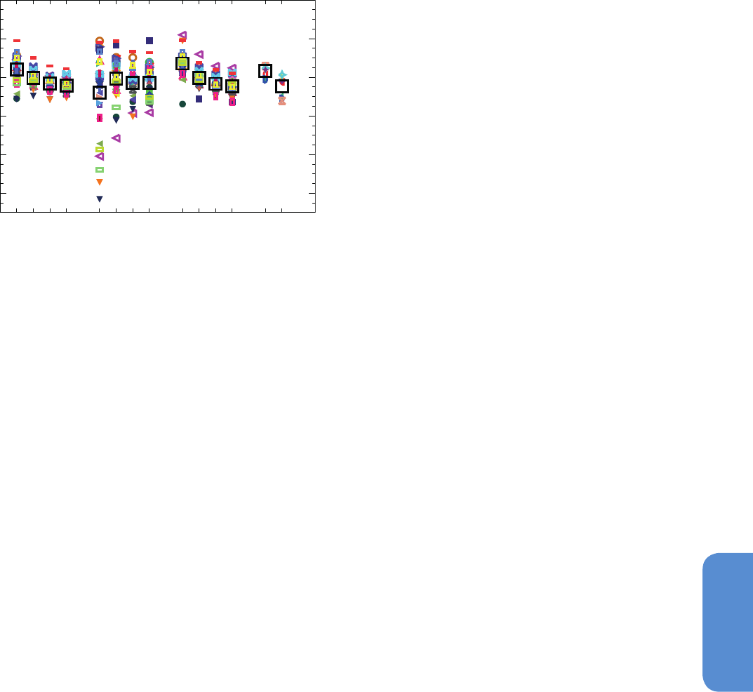
1057

Long-term Climate Change: Projections, Commitments and Irreversibility Chapter 12

Figure 12.7 | Percentage changes over the 21st century in global, land and ocean pre-

cipitation per degree Celsius of global warming in CMIP5 model concentration-driven

projections for the four RCP scenarios. Annual mean changes are calculated for each

year between 2006 and 2100 from one ensemble member per model relative to its

mean precipitation and temperature for the 1986–2005 baseline period, and the gradi-

ent of a least-squares ﬁt through the annual data is derived. Land and ocean derived

values use global mean temperature in the denominator of dP/dT. Each coloured

symbol represents a different model, the same symbol being used for the same model

for different RCPs and larger black squares being the multi-model mean. Also shown

for comparison are global mean results for ENSEMBLES model concentrations-driven

projections for the E1 and A1B scenarios (Johns et al., 2011), in this case using a least-

squares ﬁt derived over the period 2000–2099 and taking percentage changes relative

to the 1980–1999 baseline period. Changes of precipitation over land and ocean are

discussed in Section 12.4.5.2.

observational studies suggest precipitation sensitivity values higher

than model estimates (Wentz et al., 2007; Zhang et al., 2007), although

more recent studies suggest consistent values (Adler et al., 2008; Li et

al., 2011b).

12.4.1.2 Uncertainties in Global Quantities

Uncertainties in global mean quantities arise from variations in internal

natural variability, model response and forcing pathways. Table 12.2

gives two measures of uncertainty in the CMIP5 model projections,

the standard deviation and the 5 to 95% range across the ensemble’s

distribution. Because CMIP5 was not designed to explore fully the

uncertainty range in projections (see Section 12.2), neither its stand-

ard deviation nor its range can be interpreted directly as an uncer-

tainty statement about the corresponding real quantities, and other

techniques and arguments to assess uncertainty in future projections

must be considered. Figure 12.8 summarizes the uncertainty ranges

in global mean temperature changes at the end of the 21st century

under the various scenarios quantiﬁed by various methods. Individual

CMIP5 models are shown by red crosses. Red bars indicate mean and

5 to 95% percentiles based on assuming a normal distribution for the

CMIP5 sample (i.e., ±1.64 standard deviations). Estimates from the

simple climate carbon cycle Model for the Assessment of Greenhouse

Gas-Induced Climate Change (MAGICC; Meinshausen et al., 2011a;

Meinshausen et al., 2011b) calibrated to C

MIP (Friedlingstein et al.,

2006) carbon cycle models, assuming a PDF for climate sensitivity that

corresponds to the assessment of IPCC AR4 (Meehl et al., 2007b, Box

10.2), are given as yellow bars (Rogelj et al., 2012). Note that not all

2.6 4.5 6.0 8.5 2.6 4.5 6.0 8.5 2.6 4.5 6.0 8.5 E1 A1B

-4

-2

dP/dT (% °C

-1

)

CMIP5

Global

CMIP5

Land

CMIP5

Ocean

ENSEMBLES

Global

RCPRCP RCP

models have simulated all scenarios. To test the effect of undersam-

pling, and to generate a consistent set of uncertainties across scenarios,

a step response method that estimates the total warming as sum of

responses to small forcing steps (Good et al., 2011a) is used to emulate

23 CMIP5 models under the different scenarios (those 23 models that

supplied the necessary simulations to compute the emulators, i.e., CO

step change experiments). This provides means and ranges (5 to 95%)

that are comparable across scenarios (blue). See also Section 12.4.9 for

a discussion focussed on the differences between CMIP3 and CMIP5

projections of global average temperature changes.

For the CO

concentration-driven simulations (Figure 12.8a), the dom-

inant driver of uncertainty in projections of global temperature for the

higher RCPs beyond 2050 is the transient climate response (TCR), for

RCP2.6, which is closer to equilibrium by the end of the century, it is

both the TCR and the equilibrium climate sensitivity (ECS). In a tran-

sient situation, the ratio of temperature to forcing is approximately

constant and scenario independent (Meehl et al., 2007b, Appendix

10.A.1; Gregory and Forster, 2008; Knutti et al., 2008b; Good et al.,

2013). Therefore, the uncertainty in TCR maps directly into the uncer-

tainty in global temperature projections for the RCPs other than

RCP2.6. The assessed likely range of TCR based on various lines of

evidence (see Box 12.2) is similar to the 5 to 95% percentile range

of TCR in CMIP5. In addition, the assessed likely range of ECS is also

consistent with the CMIP5 range (see Box 12.2). There is little evidence

that the CMIP5 models are signiﬁcantly over- or underestimating the

RF. The RF uncertainty is small compared to response uncertainty (see

Figure 12.4), and is considered by treating the 5 to 95% as a likely

rather than very likely range. Kuhlbrodt and Gregory (2012) suggest

that models might be overestimating ocean heat uptake, as previously

suggested by Forest et al. (2006), but observationally constrained esti-

mates of TCR are unaffected by that. The ocean heat uptake efﬁciency

does not contribute much to the spread of TCR (Knutti and Tomassini,

2008; Kuhlbrodt and Gregory, 2012).

Therefore, for global mean temperature projections only, the 5 to 95%

range (estimated as 1.64 times the sample standard deviation) of the

CMIP5 projections can also be interpreted as a likely range for future

temperature change between about 2050 and 2100. Conﬁdence in this

assessment is high for the end of the century because the warming

then is dominated by CO

and the TCR. Conﬁdence is only medium for

mid-century when the contributions of RF and initial conditions to the

total temperature response uncertainty are larger. The likely ranges are

an expert assessment, taking into account many lines of evidence, in

much the same way as in AR4 (Figure SPM.5), and are not probabilistic.

The likely ranges for 2046–2065 do not take into account the possible

inﬂuence of factors that lead to near-term (2016–2035) projections of

global mean surface temperature (GMST) that are somewhat cooler

than the 5 to 95% model ranges (see Section 11.3.6), because the

inﬂuence of these factors on longer term projections cannot be quan-

tiﬁed. A few recent studies indicate that some of the models with the

strongest transient climate response might overestimate the near term

warming (Otto et al., 2013; Stott et al., 2013) (see Sections 10.8.1,

11.3.2.1.1), but there is little evidence of whether and how much that

affects the long-term warming response. One perturbed physics ensem-

ble combined with observations indicates warming that exceeds the

AR4 at the top end but used a relatively short time period of warming

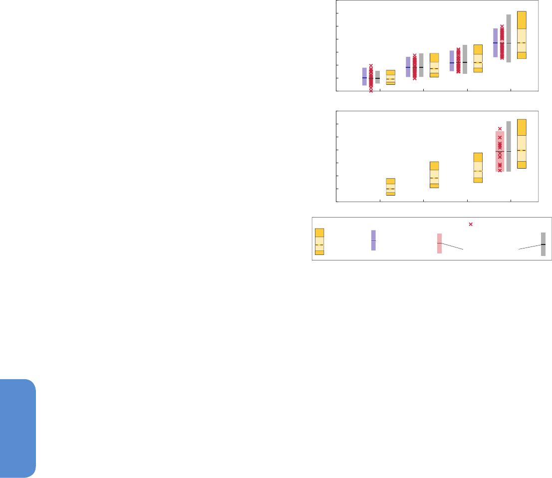
1058

Chapter 12 Long-term Climate Change: Projections, Commitments and Irreversibility

(50 years) to constrain the models’ projections (Rowlands et al., 2012)

(see Sections 11.3.2.1.1 and 11.3.6.3). GMSTs for 2081–2100 (rela-

tive to 1986–2005) for the CO

concentration driven RCPs is therefore

assessed to likely fall in the range 0.3°C to 1.7°C (RCP2.6), 1.1°C to

2.6°C (RCP4.5), 1.4°C to 3.1°C (RCP6.0), and 2.6°C to 4.8°C (RCP8.5)

estimated from CMIP5. Beyond 2100, the number of CMIP5 simula-

tions is insufﬁcient to estimate a likely range. Uncertainties before

2050 are assessed in Section 11.3.2.1.1. The assessed likely range is

very similar to the range estimated by the pulse response model, sug-

gesting that the different sample of models for the different RCPs are

not strongly affecting the result, and providing further support that

this pulse response technique can be used to emulate temperature and

ocean heat uptake in Chapter 13 and Section 12.4.9. The results are

consistent with the probabilistic results from MAGICC, which for the

lower RCPs have a slightly narrower range due to the lack of inter-

nal variability in the simple model, and the fact that non-CO

forcings

are treated more homogeneously than in CMIP5 (Meinshausen et al.,

2011a, 2011b). This is particularly pronounced for RCP2.6 where the

CMIP5 range is substantially larger, partly due to the larger fraction of

non-CO

forcings in that scenario.

The uncertainty estimate in AR4 for the SRES scenarios was –40% to

+60% around the CMIP3 means (shown here in grey for comparison).

That range was asymmetric and wider for the higher scenarios because

it included the uncertainty in carbon cycle climate feedbacks. The SRES

scenarios are based on the assumption of prescribed emissions, which

then translates to uncertainties in concentrations that propagate

through to uncertainties in the temperature response. The RCP sce-

narios assume prescribed concentrations. For scenarios that stabilize

(RCP2.6) that approach of constant fractional uncertainty underes-

timates the uncertainty and is no longer applicable, mainly because

internal variability has a larger relative contribution to the total uncer-

tainty (Good et al., 2013; Knutti and Sedláček, 2013). For the RCPs,

the carbon cycle climate feedback uncertainty is not included because

the simulations are driven by concentrations. Furthermore, there is no

clear evidence that distribution of CMIP5 global temperature changes

deviates from a normal distribution. For most other variables the shape

of the distribution is unclear, and standard deviations are simply used

as an indication of model spread, not representing a formal uncertainty

assessment.

Simulations with prescribed CO

emissions rather than concentrations

are only available for RCP8.5 (Figure 12.8b) and from MAGICC. The

projected temperature change in 2100 is slightly higher and the uncer-

tainty range is wider as a result of uncertainties in the carbon cycle

climate feedbacks. The CMIP5 range is consistent with the uncertainty

range given in AR4 for SRES A2 in 2100. Further details about emission

versus concentration driven simulations are given in Section 12.4.8.

In summary, the projected changes in global temperature for 2100 in

the RCP scenarios are very consistent with those obtained by CMIP3

for SRES in IPCC AR4 (see Section 12.4.9) when taking into account the

differences in scenarios. The likely uncertainty ranges provided here are

similar for RCP4.5 and RCP6.0 but narrower for RCP8.5 compared to

AR4. There was no scenario as low as RCP2.6 in AR4. The uncertainties

in global temperature projections have not decreased signiﬁcantly in

CMIP5 (Knutti and Sedláček, 2013), but the assessed ranges cannot be

compared between AR4 and AR5. The main reason is that uncertain-

ties in carbon cycle feedbacks are not considered in the concentration

driven RCPs. In contrast, the likely range in AR4 included those. The

assessed likely ranges are therefore narrower for the high RCPs. The

differences in the projected warming are largely attributable to the dif-

ference in scenarios (Knutti and Sedláček, 2013), and the change in the

future and reference period, rather than to developments in modelling

since AR4. A detailed comparison between the SRES and RCP scenarios

and the CMIP3 and CMIP5 models is given in Section 12.4.9.

12.4.2 Pattern Scaling

12.4.2.1 Deﬁnition and Use

In this chapter we show geographical patterns of projected changes

in climate variables according to speciﬁc scenarios and time horizons.

Alternative scenarios and projection times can be inferred from those

shown by using some established approximation methods. This is espe-

cially the case for large-scale regional patterns of average temperature

and—with additional caveats—precipitation changes. In fact, ‘pattern

scaling’ is an approximation that has been explicitly suggested in the

description of the RCPs (Moss et al., 2010) as a method for deriving

impact-relevant regional projections for scenarios that have not been

simulated by global and regional climate models. It was ﬁrst proposed

RCP2.6 RCP4.5 RCP6.0 RCP8.5

Concentration-driven

RCP2.6 RCP4.5 RCP6.0 RCP8.5

Emission-driven

CMIP5 models

90% range

66% range

median

Rogelj et al. 2012 Good et al. 2011

multimodel mean

-40 to +60% range

around mean

likely range

50th percentile

5-95th perc. range

Temperature increase in 2081-2100

relative to 1986 to 2005 (°C)

Temperature increase in 2081-2100

relative to 1986 to 2005 (°C)

Figure 12.8 | Uncertainty estimates for global mean temperature change in 2081–

2100 with respect to 1986–2005. Red crosses mark projections from individual CMIP5

models. Red bars indicate mean and 5 to 95% ranges based on CMIP5 (1.64 standard

deviations), which are considered as a likely range. Blue bars indicate 5 to 95% ranges

from the pulse response emulation of 21 models (Good et al., 2011a). Grey bars mark

the range from the mean of CMIP5 minus 40% to the mean +60%, assessed as likely in

AR4 for the SRES scenarios. The yellow bars show the median, 17 to 83% range and 5

to 95% range based on Rogelj et al. (2012). See also Figures 12.39 and 12.40.

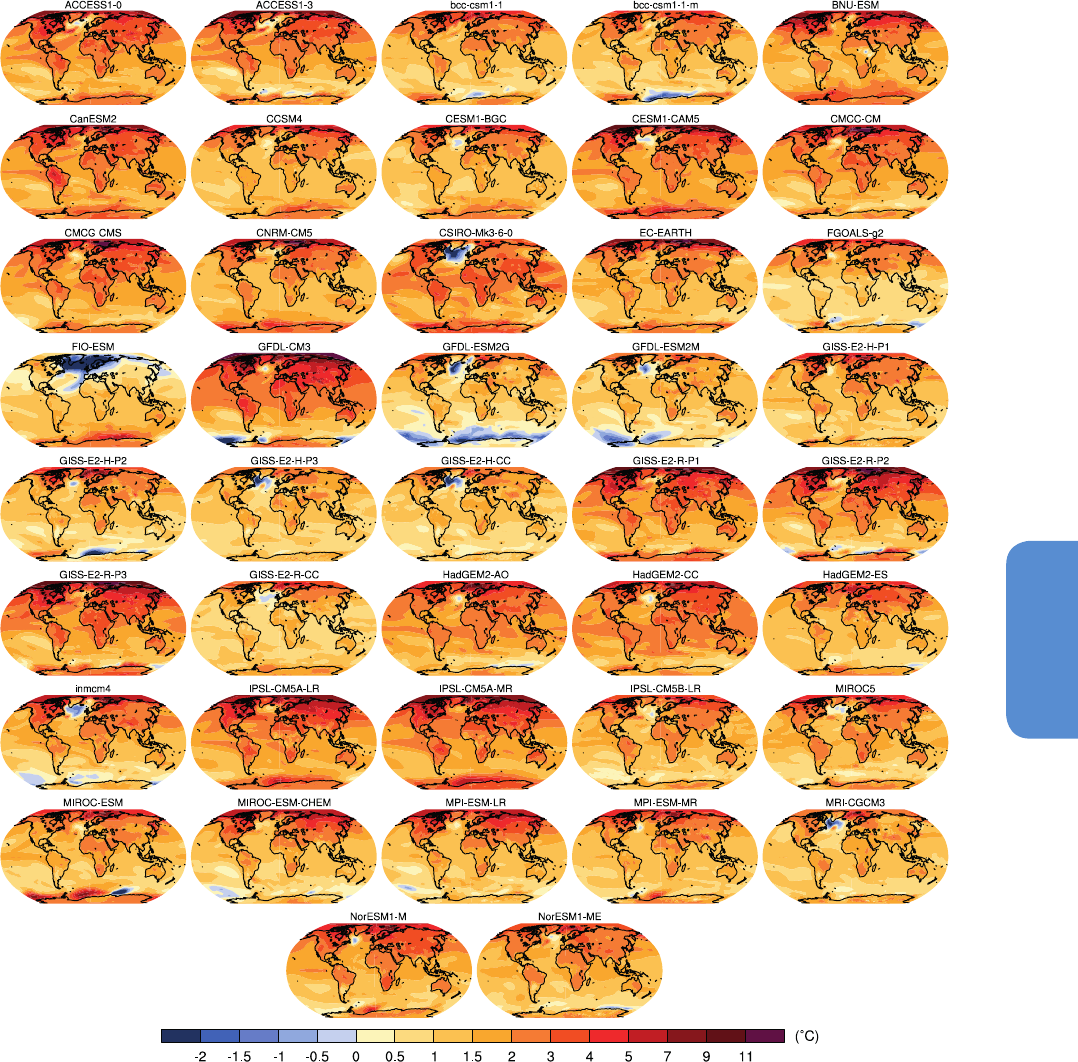
1059

Long-term Climate Change: Projections, Commitments and Irreversibility Chapter 12

Figure 12.9 | Surface air temperature change in 2081–2100 displayed as anomalies with respect to 1986–2005 for RCP4.5 from one ensemble member of each of the concen-

tration-driven models available in the CMIP5 archive.

Annual mean surface air temperature change (RCP4.5: 2081-2100)

by Santer et al. (1990) and revisited later by numerous studies (e.g.,

Huntingford and Cox, 2000). It relies on the existence of robust geo-

graphical patterns of change, emerging at the time when the response

to external forcings emerges from the noise, and persisting across the

length of the simulation, across different scenarios, and even across

models, modulated by the corresponding changes in global average

temperature. The robustness of temperature change patterns has

been amply documented from the original paper onward. An example

is given in Figure 12.9 for surface air temperature from each of the

CMIP5 models highlighting both similarities and differences between

the responses of different models. The precipitation pattern was shown

to scale linearly with global average temperature to a sufﬁcient accu-

racy in CMIP3 models (Neelin et al., 2006) for this to be useful for

projections related to the hydrological cycle. Shiogama et al. (2010b)

ﬁnd similar results with the caution that in the early stages of warming

aerosols modify the pattern. A more mixed evaluation can be found in

1060

Chapter 12 Long-term Climate Change: Projections, Commitments and Irreversibility

Good et al. (2012), where some land areas in the low latitudes exhibit a

nonlinear relation to global average temperature, but, largely, average

precipitation change over the remaining regions can be well approx-

imated by a grid-point speciﬁc linear function of global average tem-

perature change. It is in the latter quantity that the dependence of the

evolution of the change in time on the model (e.g., its climate sensitivi-

ty) and the forcing (e.g., the emission scenario) is encapsulated.

In analytical terms, it is assumed that the following relation holds:

C (t,x) = T

(t) c(x) + R (t, x)

where the symbol x identiﬁes the geographic location (model grid

point or other spatial coordinates) and possibly the time of year (e.g.,

a June–July–August average). The index t runs along the length of the

forcing scenario of interest. T

(t) indicates global average temperature

change at time t under this scenario; c(x) is the time-invariant geo-

graphic pattern of change per 1°C global surface temperature change

for the variable of interest (which represents the forced component of

the change) and C (t,x) is the actual ﬁeld of change for that variable

at the speciﬁc time t under this scenario. The R (t, x) is a residual term

and highlights the fact that pattern scaling cannot reconstruct model

behaviour with complete accuracy due to both natural variability and

because of limitations of the methodology discussed below. This way,

regionally and temporally differentiated results under different scenar-

ios or climate sensitivities can be approximated by the product of a

spatial pattern, constant over time, scenario and model characteristics,

and a time evolving global mean change in temperature. Model and

scenario dependence are thus captured through the global mean tem-

perature response, and simple climate models calibrated against fully

coupled climate models can be used to simulate the latter, at a great

saving in computational cost. The spatial pattern can be estimated

through the available coupled model simulations under the assump-

tion that it does not depend on the speciﬁc scenario(s) used.

The choice of the pattern in the studies available in the literature can be

as simple as the ensemble average ﬁeld of change (across models and/

or across scenarios, for the coupled experiments available), normalized

by the corresponding change in global average temperature, choosing

a segment of the simulations when the signal has emerged from the

noise of natural variability from a baseline of reference (e.g., the last

20 years of the 21st century compared to pre-industrial or current cli-

mate) and taking the difference of two multi-decadal means. Similar

properties and results have been obtained using more sophisticated

multivariate procedures that optimize the variance explained by the

pattern (Holden and Edwards, 2010). The validity of this approximation

is discussed by Mitchell et al. (1999) and Mitchell (2003). Huntingford

and Cox (2000) evaluate the quality of the approximation for numer-

ous variables, showing that the technique performs best for temper-

ature, downward longwave radiation, relative humidity, wind speeds

and surface pressure while showing relatively larger limitations for

rainfall rate anomalies. Joshi et al. (2013) have recently shown that the

accuracy of the approximation, especially across models, is improved

by adding a second term, linear in the land–sea surface warming ratio,

another quantity that can be easily estimated from existing coupled

climate model simulations. There exist of course differences between

the patterns generated by different GCMs (documented for example

for CMIP3 in Watterson and Whetton, 2011b), but uncertainty can be

characterized, for example, by the inter-model spread in the pattern

c(x). Recent applications of the methodology to probabilistic future

projections have in fact sought to fully quantify errors introduced by

the approximation, on the basis of the available coupled model runs

(Harris et al., 2006).

Pattern scaling and its applications have been documented in IPCC

WGI Reports before (IPCC, 2001, Section 13.5.2.1; Meehl et al., 2007b,

Section 10.3.2). It has been used extensively for regional tempera-

ture and precipitation change projections, for example, Murphy et al.

(2007), (Watterson, 2008), Giorgi (2008), Harris et al. (2006, 2010), May

(2008a), Ruosteenoja et al. (2007), Räisänen and Ruokolainen (2006),

Cabre et al. (2010) and impact studies, for example, as described in

Dessai et al. (2005) and Fowler et al. (2007b). Recent studies have

focussed on patterns linked to warming at certain global average tem-

perature change thresholds (e.g., May, 2008a; Sanderson et al., 2011)

and patterns derived under the RCPs (Ishizaki et al., 2012).

There are basic limitations to this approach, besides a degradation of

its performance as the regional scale of interest becomes ﬁner and in

the presence of regionally speciﬁc forcings. Recent work with MIROC3.2

(Shiogama et al., 2010a; Shiogama et al., 2010b) has revealed a depend-

ence of the precipitation sensitivity (global average precipitation change

per 1°C of global warming—see Figure 12.6) on the scenario, due to the

precipitation being more sensitive to carbon aerosols than WMGHGs.

In fact, there are signiﬁcant differences in black and organic carbon

aerosol forcing between the emission scenarios investigated by Shiog-

ama et al. (2010a; 2010b). Levy II et al. (2013) conﬁrm that patterns of

precipitation change are spatially correlated with the sources of aerosol

emissions, in simulations where the indirect effect is represented. This

is a behaviour that is linked to a more general limitation of pattern

scaling, which breaks down if aerosol forcing is signiﬁcant. The effects

of aerosols have a regional nature and are thus dependent on the future

sources of pollution which are likely to vary geographically in the future

and are difﬁcult to predict (May, 2008a). For example, Asian and North

American aerosol production are likely to have different time histories

and future projections. Schlesinger et al. (2000) extended the method-

ology of pattern scaling by isolating and recombining patterns derived

by dedicated experiments with a coupled climate model where sulphate

aerosols were increased for various regions in turn. More recently, in

an extension of pattern scaling into a probabilistic treatment of model,

scenario and initial condition uncertainties, Frieler et al. (2012) derived

joint probability distributions for regionally averaged temperature and

precipitation changes as linear functions of global average temperature

and additional predictors including regionally speciﬁc sulphate aerosol

and black carbon emissions.

Pattern scaling is less accurate for strongly mitigated stabilization

scenarios. This has been shown recently by May (2012), compar-

ing patterns of temperature change under a scenario limiting global

warming since pre-industrial times to 2°C and patterns produced by

a scenario that reaches 4.5°C of global average temperature change.

The limitations of pattern scaling in approximating changes while the

climate system approaches equilibrium have found their explanation in

Manabe and Wetherald (1980) and Mitchell et al. (1999). Both studies

point out that as the temperatures of the deep oceans reach equilibri-

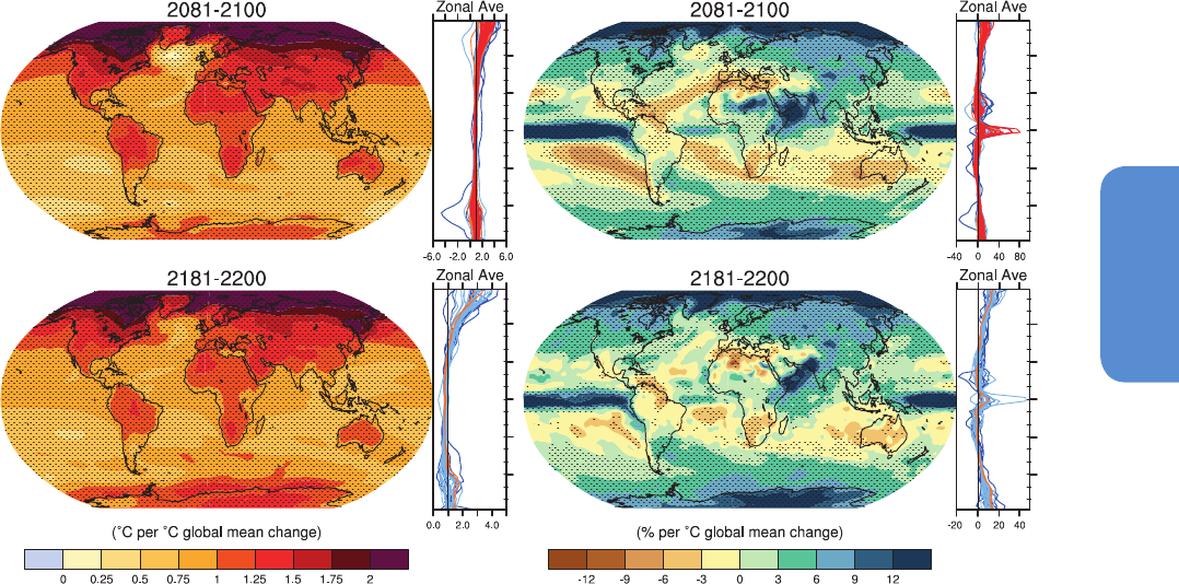
1061

Long-term Climate Change: Projections, Commitments and Irreversibility Chapter 12

um (over multiple centuries) the geographical distribution of warming

changes as well, for example, showing a larger warming of the high

latitudes in the SH than in the earlier periods of the transient response,

relative to the global mean warming. More recently, Held et al. (2010)

showed how this slow warming pattern is in fact present during the

initial transient response of the system as well, albeit with much small-

er amplitude. Further, Gillett et al. (2011) show how in a simulation in

which emissions cease, regional temperatures and precipitation pat-

terns exhibit ongoing changes, even though global mean temperature

remains almost constant. Wu et al. (2010) showed that the global pre-

cipitation response shows a nonlinear response to strong mitigation

scenarios, with the hydrological cycle continuing to intensify even after

atmospheric CO

concentration, and thus global average temperature,

start decreasing. Regional nonlinear responses to mitigation scenari-

os of precipitation and sea surface temperatures (SSTs) are shown by

Chadwick et al. (2013).

Other areas where pattern scaling shows a lack of robustness are the

edges of polar ice caps and sea ice extent, where at an earlier time in

the simulation ice melts and regions of sharp gradient surface, while

later in the simulation, in the absence of ice, the gradient will become

less steep. Different sea ice representations in models also make the

location of such regions much less robust across the model ensembles

and the scenarios.

Pattern scaling has not been as thoroughly explored for quantities

other than average temperature and precipitation. Impact relevant

extremes, for example, seem to indicate a critical dependence on the

scale at which their changes are evaluated, with studies showing that

some aspects of their statistics change in a close-to-linear way with

mean temperature (Kharin et al., 2007; Lustenberger et al., 2013) while

others have documented the dependence of their changes on moments

of their statistical distribution other than the mean (Ballester et al.,

2010a), which would make pattern scaling inadequate.

12.4.2.2 Coupled Model Intercomparison Project Phase 5 Patterns

Scaled by Global Average Temperature Change

On the basis of CMIP5 simulations, we show geographical patterns

(Figure 12.10) of warming and precipitation change and indicate

measures of their variability across models and across RCPs. The pat-

terns are scaled to 1°C global mean surface temperature change above

the reference period 1986–2005 for 2081–2100 (ﬁrst row) and for a

period of approximate stable temperature, 2181–2200 (thus excluding

RCP8.5, which does not stabilize by that time) (second row). Spatial

correlation of ﬁelds of temperature and precipitation change range

from 0.93 to 0.99 when considering ensemble means under different

RCPs. The lower values are found when computing correlation between

RCP2.6 and the higher RCPs, and may be related to the high mitigation

Precipitation scaled by global T (% per

C)Temperature scaled by global T (

C per

Figure 12.10 | Temperature (left) and precipitation (right) change patterns derived from transient simulations from the CMIP5 ensembles, scaled to 1°C of global mean surface

temperature change. The patterns have been calculated by computing 20-year averages at the end of the 21st (top) and 22nd (bottom) centuries and over the period 1986–2005

for the available simulations under all RCPs, taking their difference (percentage difference in the case of precipitation) and normalizing it, grid-point by grid-point, by the cor-

responding value of global average temperature change for each model and scenario. The normalized patterns have then been averaged across models and scenarios. The colour

scale represents degrees Celsius (in the case of temperature) and percent (in the case of precipitation) per 1°C of global average temperature change. Stippling indicates where the

mean change averaged over all realizations is larger than the 95% percentile of the distribution of models. Zonal means of the geographical patterns are shown for each individual

model for RCP2.6 (blue), 4.5 (light blue), 6.0 (orange) and 8.5 (red). RCP8.5 is excluded from the stabilization ﬁgures. The RCP2.6 simulation of the FIO-ESM (First Institute of

Oceanography) model was excluded because it did not show any warming by the end of the 21st century, thus not complying with the method requirement that the pattern be

estimated at a time when the temperature change signal from CO

increase has emerged.

1062

Chapter 12 Long-term Climate Change: Projections, Commitments and Irreversibility

enacted under RCP2.6 from early in the 21st century. Pattern corre-

lation varies between 0.91 and 0.98 for temperature and between

0.91 and 0.96 for precipitation when comparing patterns computed

by averaging and normalizing changes at the end of the 21st, 22nd

and 23rd centuries, with the largest value representing the correlation

between the patterns at the end of the 22nd and 23rd centuries, the

lowest representing the correlation between the pattern at the end

of the 21st and the pattern at the end of the 23rd century. The zonal

means shown to the side of each plot represent each model by one line,

colour coding the four different scenarios. They show good agreement

of models and scenarios over low and mid-latitudes for temperature,

but higher spread across models and especially across scenarios for the

areas subject to polar ampliﬁcation, for which the previous discussion

about the sensitivity of the patterns to the sea ice edge may be rele-

vant. A comparison of the mean of the lines to their spread indicates

overall the presence of a strong mean signal with respect to the spread

of the ensemble. Precipitation shows an opposite pattern of inter-mod-

el spread, with larger variations in the low latitudes and around the

equator, and smaller around the high latitudes. Precipitation has also

a lower signal-to-noise ratio (measured as above by comparing the

ensemble mean change magnitude to the spread across models and

scenarios of these zonal mean averages).

As already mentioned, although we do not explicitly use pattern scaling

in the sections that follow, we consider it a useful approximation when

the need emerges to interpolate or extrapolate results to different sce-

narios or time periods, noting the possibility that the scaling may break

down at higher levels of global warming, and that the validity of the

approximation is limited to broad patterns of change, as opposed to

local scales. An important caveat is that pattern scaling only applies

to the climate response that is externally forced. The actual response

is a combination of forced change and natural variability, which is not

and should not be scaled up or down by the application of this tech-

nique, which becomes important on small spatial scales and shorter

time scales, and whose relative magnitude compared to the forced

component also depends on the variable (Hawkins and Sutton, 2009,

2011; Mahlstein et al., 2011; Deser et al., 2012a, 2012b; Mahlstein et

al., 2012) (see Section 11.2). One approach to produce projections that

include both components is to estimate natural variability separately,

scale the forced response and add the two.

12.4.3 Changes in Temperature and Energy Budget

12.4.3.1 Patterns of Surface Warming: Land–Sea Contrast,

Polar Ampliﬁcation and Sea Surface Temperatures

Patterns of surface air temperature change for various RCPs show

widespread warming during the 21st century (Figure 12.11; see

Annex I for seasonal patterns). A key feature that has been present

throughout the history of coupled modelling is the larger warming over

land compared to oceans, which occurs in both transient and equilib-

rium climate change (e.g., Manabe et al., 1990). The degree to which

warming is larger over land than ocean is remarkably constant over

time under transient warming due to WMGHGs (Lambert and Chiang,

2007; Boer, 2011; Lambert et al., 2011) suggesting that heat capac-

ity differences between land and ocean do not play a major role in

the land–sea warming contrast (Sutton et al., 2007; Joshi et al., 2008,

2013). The phenomenon is predominantly a feature of the surface and

lower atmosphere (Joshi et al., 2008). Studies have found it occurs due

to contrasts in surface sensible and latent ﬂuxes over land (Sutton et

al., 2007), land–ocean contrasts in boundary layer lapse rate changes

(Joshi et al., 2008), boundary layer relative humidity and associated

low-level cloud cover changes over land (Doutriaux-Boucher et al.,

2009; Fasullo, 2010) and soil moisture reductions (Dong et al., 2009;

Clark et al., 2010) under climate change. The land–sea warming con-

trast is also sensitive to aerosol forcing (Allen and Sherwood, 2010;

Joshi et al., 2013). Globally averaged warming over land and ocean

is identiﬁed separately in Table 12.2 for the CMIP5 models and the

ratio of land to ocean warming is likely in the range of 1.4 to 1.7,

consistent with previous studies (Lambert et al., 2011). The CMIP5 mul-

ti-model mean ratio is approximately constant from 2020 through to

2100 (based on an update of Joshi et al., 2008 from available CMIP5

models).

Ampliﬁed surface warming in Arctic latitudes is also a consistent fea-

ture in climate model integrations (e.g., Manabe and Stouffer, 1980).

This is often referred to as polar ampliﬁcation, although numerous

studies have shown that under transient forcing, this is primarily an

Arctic phenomenon (Manabe et al., 1991; Meehl et al., 2007b). The

lack of an ampliﬁed transient warming response in high Southern polar

latitudes has been associated with deep ocean mixing, strong ocean

heat uptake and the persistence of the vast Antarctic ice sheet. In equi-

librium simulations, ampliﬁed warming occurs in both polar regions.

On an annual average, and depending on the forcing scenario (see

Table 12.2), the CMIP5 models show a mean Arctic (67.5°N to 90°N)

warming between 2.2 and 2.4 times the global average warming for

2081–2100 compared to 1986–2005. Similar polar ampliﬁcation fac-

tors occurred in earlier coupled model simulations (e.g., Holland and

Bitz, 2003; Winton, 2006a). This factor in models is slightly higher

than the observed central value, but it is within the uncertainty of

the best estimate from observations of the recent past (Bekryaev et

al., 2010). The uncertainty is large in the observed factor because sta-

tion records are short and sparse (Serreze and Francis, 2006) and the

forced signal is contaminated by the noise of internal variability. By

contrast, model trends in surface air temperature are 2.5 to 5 times

higher than observed over Antarctica, but here also the observational

estimates have a very large uncertainty, so, for example, the CMIP3

ensemble mean is consistent with observations within error estimates

(Monaghan et al., 2008). Moreover, recent work suggests more wide-

spread current West Antarctic surface warming than previously esti-

mated (Bromwich et al., 2013).

The ampliﬁed Arctic warming in models has a distinct seasonal charac-

ter (Manabe and Stouffer, 1980; Rind, 1987; Holland and Bitz, 2003; Lu

and Cai, 2009; Kumar et al., 2010). Arctic ampliﬁcation (deﬁned as the

67.5 N° to 90°N warming compared to the global average warming

for 2081–2100 versus 1986–2005) peaks in early winter (November

to December) with a CMIP5 RCP4.5 multi-model mean warming for

67.5°N to 90°N exceeding the global average by a factor of more than

4. The warming is smallest in summer when excess heat at the Arctic

surface goes into melting ice or is absorbed by the ocean, which has

a relatively large thermal inertia. Simulated Arctic warming also has

a consistent vertical structure that is largest in the lower troposphere

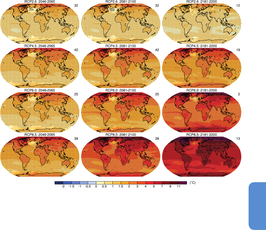
1063

Long-term Climate Change: Projections, Commitments and Irreversibility Chapter 12

(e.g., Manabe et al., 1991; Kay et al., 2012). This is in agreement with

recent observations (Serreze et al., 2009; Screen and Simmonds, 2010)

but contrary to an earlier study that suggested a larger warming aloft

(Graversen et al., 2008). The discrepancy in observed vertical structure

may reﬂect inadequacies in data sets (Bitz and Fu, 2008; Grant et al.,

2008; Thorne, 2008) and sensitivity to the time period used for averag-

ing (see also Box 2.3).

As also discussed in Box 5.1, there are many mechanisms that con-

tribute to Arctic ampliﬁcation, some of which were identiﬁed in early

modelling studies (Manabe and Stouffer, 1980). Feedbacks associat-

ed with changes in sea ice and snow amplify surface warming near

the poles (Hall, 2004; Soden et al., 2008; Graversen and Wang, 2009;

Kumar et al., 2010). The longwave radiation changes in the top of the

atmosphere associated with surface warming opposes surface warm-

ing at all latitudes, but less so in the Arctic (Winton, 2006a; Soden et

al., 2008). Rising temperature globally is expected to increase the hori-

Annual mean surface air temperature change

Figure 12.11 | Multi-model ensemble average of surface air temperature change (compared to 1986–2005 base period) for 2046–2065, 2081–2100, 2181–2200 for RCP2.6,

4.5, 6.0 and 8.5. Hatching indicates regions where the multi-model mean change is less than one standard deviation of internal variability. Stippling indicates regions where the

multi-model mean change is greater than two standard deviations of internal variability and where at least 90% of the models agree on the sign of change (see Box 12.1). The

number of CMIP5 models used is indicated in the upper right corner of each panel.

zontal latent heat transport by the atmosphere into the Arctic (Flan-

nery, 1984; Alexeev et al., 2005; Cai, 2005; Langen and Alexeev, 2007;

Kug et al., 2010), which warms primarily the lower troposphere. On

average, CMIP3 models simulate enhanced latent heat transport (Held

and Soden, 2006), but north of about 65°N, the sensible heat transport

declines enough to more than offset the latent heat transport increase

(Hwang et al., 2011). Increased atmospheric heat transport into the

Arctic and subsidence warming has been associated with a teleconnec-

tion driven by enhanced convection in the tropical western Paciﬁc (Lee

et al., 2011). Ocean heat transport plays a role in the simulated Arctic

ampliﬁcation, with both large late 20th century transport (Mahlstein

and Knutti, 2011) and increases over the 21st century (Hwang et al.,

2011; Bitz et al., 2012) associated with higher ampliﬁcation. As noted

by Held and Soden (2006), Kay et al. (2012), and Alexeev and Jackson

(2012), diagnosing the role of various factors in ampliﬁed warming is

complicated by coupling in the system in which local feedbacks inter-

act with poleward heat transports.

1064

Chapter 12 Long-term Climate Change: Projections, Commitments and Irreversibility

Although models consistently exhibit Arctic ampliﬁcation as global

mean temperatures rise, the multitude of physical processes described

above mean that they differ considerably in the magnitude. Previous

work has implicated variations across climate models in numerous fac-

tors including inversion strength (Boé et al., 2009a), ocean heat trans-

port (Holland and Bitz, 2003; Mahlstein and Knutti, 2011), albedo feed-

back (Winton, 2006a), longwave radiative feedbacks (Winton, 2006a)

and shortwave cloud feedback (Crook et al., 2011; Kay et al., 2012)

as playing a role in the across-model scatter in polar ampliﬁcation.

The magnitude of ampliﬁcation is generally higher in models with less

extensive late 20th century sea ice in June, suggesting that the initial

ice state inﬂuences the 21st century Arctic ampliﬁcation. The pattern

of simulated Arctic warming is also associated with the initial ice state,

and in particular with the location of the winter sea ice edge (Holland

and Bitz, 2003; Räisänen, 2007; Bracegirdle and Stephenson, 2012).

This relationship has been suggested as a constraint on projected

Arctic warming (Abe et al., 2011; Bracegirdle and Stephenson, 2012),

although, in general, the ability of models to reproduce observed cli-

mate and its trends is not a sufﬁcient condition for attributing high

conﬁdence to the projection of future trends (see Section 9.8).

Minima in surface warming occur in the North Atlantic and Southern

Oceans under transient forcing in part due to deep ocean mixed layers

in those regions (Manabe et al., 1990; Xie et al., 2010). Trenberth and

Fasullo (2010) ﬁnd that the large biases in the Southern Ocean energy

budget in CMIP3 coupled models negatively correlate with equilibrium

climate sensitivity (see Section 12.5.3), suggesting that an improved

mean state in the Southern Ocean is needed before warming there

can be understood. In the equatorial Paciﬁc, warming is enhanced

in a narrow band which previous assessments have described as ‘El

Niño-like’, as may be expected from the projected decrease in atmos-

pheric tropical circulations (see Section 12.4.4). However, DiNezio et al.

(2009) highlight that the tropical Paciﬁc warming in the CMIP3 models

is not ‘El Niño-like’ as the pattern of warming and associated tele-

connections (Xie et al., 2010; Section 12.4.5.2) is quite distinct from

that of an El Niño event. Instead the pattern is of enhanced equatorial

warming and is due to a meridional minimum in evaporative damping

on the equator (Liu et al., 2005) and ocean dynamical changes that can

be decoupled from atmospheric changes (DiNezio et al., 2009) (see

also further discussion in Section 12.4.7).

In summary, there is robust evidence over multiple generations of

models and high conﬁdence in these large-scale warming patterns. In

the absence of a strong reduction in the Atlantic Meridional Overturn-

ing Circulation (AMOC), there is very high conﬁdence that the Arctic

region is projected to warm most.

12.4.3.2 Zonal Average Atmospheric Temperature

Zonal temperature changes at the end of the 21st century show warm-

ing throughout the troposphere and, depending on the scenario, a mix

of warming and cooling in the stratosphere (Figure 12.12). The max-

imum warming in the tropical upper troposphere is consistent with

theoretical explanations and associated with a decline in the moist

adiabatic lapse rate of temperature in the tropics as the climate warms

(Bony et al., 2006). The northern polar regions also experience large

warming in the lower atmosphere, consistent with the mechanisms

discussed in Section 12.4.3.1. The tropospheric patterns are similar

to those in the TAR and AR4 with the RCP8.5 changes being up to

several degrees warmer in the tropics compared to the A1B changes

appearing in the AR4. Similar tropospheric patterns appear in the RCP

2.6 and 4.5 changes, but with reduced magnitudes, suggesting some

degree of scaling with forcing change in the troposphere, similar to

behaviour discussed in the AR4 and Section 12.4.2. The consistency of

tropospheric patterns over multiple generations of models indicates

high conﬁdence in these projected changes.

In the stratosphere, the models show similar tropical patterns of

change, with magnitudes differing according to the degree of cli-

mate forcing. Substantial differences appear in polar regions. In the

north, RCP8.5 and 4.5 yield cooling, though it is more signiﬁcant in

the RCP8.5 ensemble. In contrast, RCP2.6 shows warming, albeit weak

and with little signiﬁcance. In the southern polar region, RCP 2.6 and

4.5 both show signiﬁcant warming, and RCP8.5 is the outlier, with sig-

niﬁcant cooling. The polar stratospheric warming, especially in the SH,

is similar to that found by Butchart et al. (2010) and Meehl et al. (2012)

in GCM simulations that showed effects of ozone recovery in deter-

mining the patterns (Baldwin et al., 2007; Son et al., 2010). Eyring et

al. (2013) ﬁnd behaviour in the CMIP5 ensemble both for models with

and without interactive chemistry that supports the contention that

the polar stratospheric changes in Figure 12.12 are strongly inﬂuenced

by ozone recovery. Overall, the stratospheric temperature changes do

not exhibit pattern scaling with global temperature change and are

dependent on ozone recovery.

Away from the polar stratosphere, there is physical and pattern consist-

ency in temperature changes between different generations of models

assessed here and in the TAR and AR4. The consistency is especially clear

in the northern high latitudes and, coupled with physical understanding,

indicates that some of the greatest warming is very likely to occur here.

There is also consistency across generations of models in relatively large

warming in the tropical upper troposphere. Allen and Sherwood (2008)

and Johnson and Xie (2010) have presented dynamic and thermody-

namic arguments, respectively, for the physical robustness of the tropi-

cal behaviour. However, there remains uncertainty about the magnitude

of warming simulated in the tropical upper troposphere because large

observational uncertainties and contradictory analyses limit a conﬁdent

assessment of model accuracy in simulating temperature trends in the

tropical upper troposphere (Section 9.4.1.4.2). The combined evidence

indicates that relatively large warming in the tropical upper troposphere

is likely, but with medium conﬁdence.

12.4.3.3 Temperature Extremes

As the climate continues to warm, changes in several types of tem-

perature extremes have been observed (Donat et al., 2013), and are

expected to continue in the future in concert with global warming

(Seneviratne et al., 2012). Extremes occur on multiple time scales, from

a single day or a few consecutive days (a heat wave) to monthly and

seasonal events. Extreme temperature events are often deﬁned by

indices (see Box 2.4 for the common deﬁnitions used), for example,

percentage of days in a year when maximum temperature is above the

90th percentile of a present day distribution or by long period return

values. Although changes in temperature extremes are a very robust

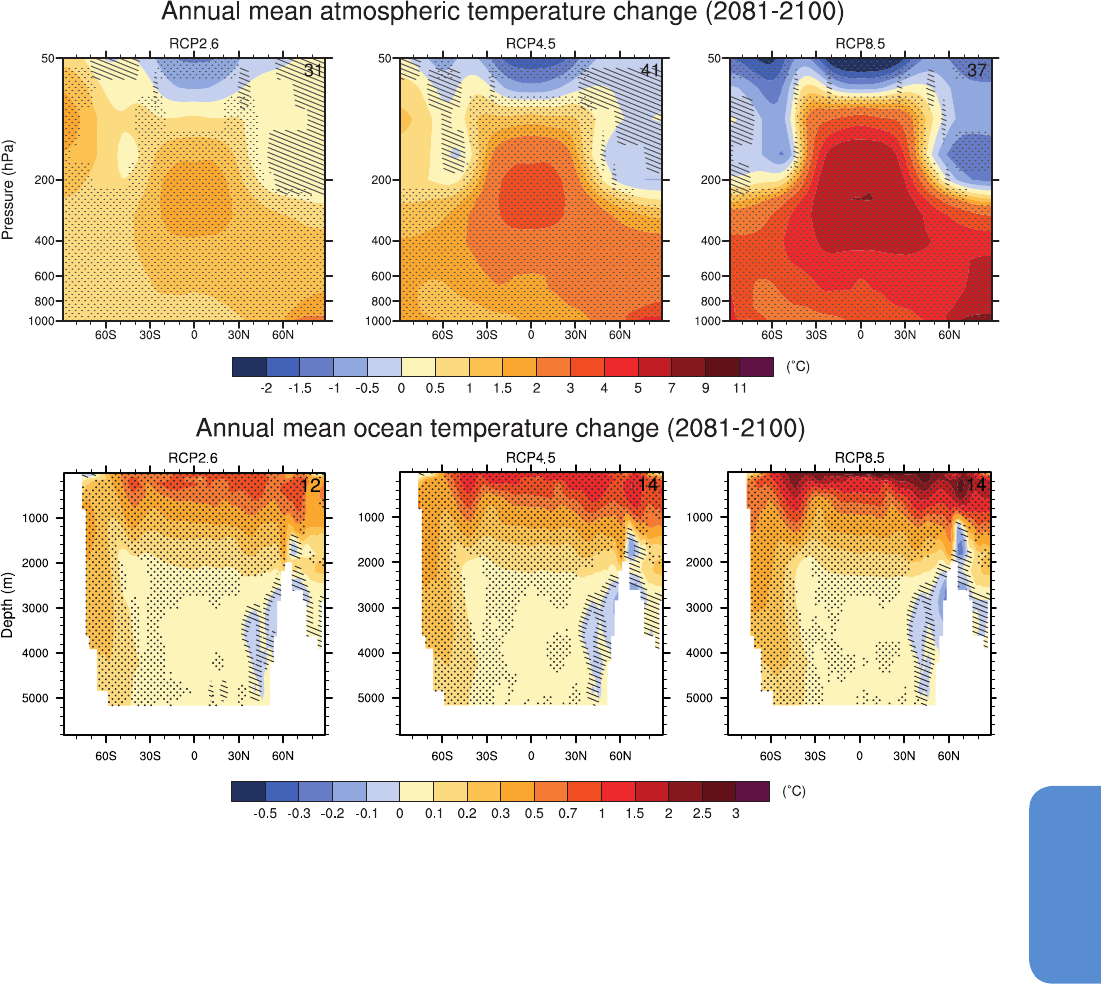
1065

Long-term Climate Change: Projections, Commitments and Irreversibility Chapter 12

signature of anthropogenic climate change (Seneviratne et al., 2012),

the magnitude of change and consensus among models varies with

the characteristics of the event being considered (e.g., time scale, mag-

nitude, duration and spatial extent) as well as the deﬁnition used to

describe the extreme.

Since the AR4 many advances have been made in establishing global

observed records of extremes (Alexander et al., 2006; Perkins et al.,

2012; Donat et al., 2013) against which models can be evaluated to

give context to future projections (Sillmann and Roeckner, 2008; Alex-

ander and Arblaster, 2009). Numerous regional assessments of future

changes in extremes have also been performed and a comprehensive

summary of these is given in Seneviratne et al. (2012). Here we sum-

marize the key ﬁndings from this report and assess updates since then.

It is virtually certain that there will be more hot and fewer cold extremes

as global temperature increases (Caesar and Lowe, 2012; Orlowsky

and Seneviratne, 2012; Sillmann et al., 2013), consistent with previous

assessments (Solomon et al., 2007; Seneviratne et al., 2012). Figure

12.13 shows multi-model mean changes in the absolute temperature

indices of the coldest day of the year and the hottest day of the year

and the threshold-based indices of frost days and tropical nights from

the CMIP5 ensemble (Sillmann et al., 2013). A robust increase in warm

temperature extremes and decrease in cold temperature extremes

is found at the end of the 21st century, with the magnitude of the

changes increasing with increased anthropogenic forcing. The coldest

night of the year undergoes larger increases than the hottest day in

the globally averaged time series (Figure 12.13b and d). This tenden-

cy is consistent with the CMIP3 model results shown in Figure 12.13,

which use different models and the SRES scenarios (see Seneviratne

et al. (2012) for earlier CMIP3 results). Similarly, increases in the fre-

quency of warm nights are greater than increases in the frequency

of warm days (Sillmann et al., 2013). Regionally, the largest increases

in the coldest night of the year are projected in the high latitudes of

Figure 12.12 | CMIP5 multi-model changes in annual mean zonal mean temperature in the atmosphere and ocean relative to 1986–2005 for 2081–2100 under the RCP2.6 (left),

RCP4.5 (centre) and RCP8.5 (right) forcing scenarios. Hatching indicates regions where the multi-model mean change is less than one standard deviation of internal variability.

Stippling indicates regions where the multi-model change mean is greater than two standard deviations of internal variability and where at least 90% of the models agree on the

sign of change (see Box 12.1).

1066

Chapter 12 Long-term Climate Change: Projections, Commitments and Irreversibility

the NH under the RCP8.5 scenario (Figure 12.13a). The subtropics and

mid-latitudes exhibit the greatest projected changes in the hottest day

of the year, whereas changes in tropical nights and the frequency of

warm days and warm nights are largest in the tropics (Sillmann et al.,

2013). The number of frost days declines in all regions while signiﬁcant

increases in tropical nights are seen in southeastern North America, the

Mediterranean and central Asia.

It is very likely that, on average, there will be more record high than

record cold temperatures in a warmer average climate. For example,

Meehl et al. (2009) ﬁnd that the current ratio of 2 to 1 for record daily

high maxima to low minima over the USA becomes approximately 20

to 1 by the mid-21st century and 50 to 1 by late century in their model

simulation of the SRES A1B scenario. However, even at the end of the

century daily record low minima continue to be broken, if in a small

number, consistent with Kodra et al. (2011), who conclude that cold

extremes will continue to occur in a warmer climate, even though their

frequency will decline.

It is also very likely that heat waves, deﬁned as spells of days with

temperature above a threshold determined from historical climatology,

will occur with a higher frequency and duration, mainly as a direct

consequence of the increase in seasonal mean temperatures (Barnett

et al., 2006; Ballester et al., 2010a, 2010b; Fischer and Schär, 2010).

Changes in the absolute value of temperature extremes are also very

likely and expected to regionally exceed global temperature increases

by far, with substantial changes in hot extremes projected even for

moderate (<2.5°C above present day) average warming levels (Clark

et al., 2010; Diffenbaugh and Ashfaq, 2010). These changes often differ

from the mean temperature increase, as a result of changes in variabili-

ty and shape of the temperature distribution (Hegerl et al., 2004; Meehl

and Tebaldi, 2004; Clark et al., 2006). For example, summer tempera-

ture extremes over central and southern Europe are projected to warm

substantially more than the corresponding mean local temperatures as

a result of enhanced temperature variability at interannual to intrasea-

sonal time scales (Schär et al., 2004; Clark et al., 2006; Kjellstrom et

al., 2007; Vidale et al., 2007; Fischer and Schär, 2009, 2010; Nikulin et

al., 2011; Fischer et al., 2012a). Several recent studies have also argued

that the probability of occurrence of a Russian heat wave at least as

severe as the one in 2010 increases substantially (by a factor of 5 to

10 by the mid-century) along with increasing mean temperatures and

enhanced temperature variability (Barriopedro et al., 2011; Dole et al.,

2011).

Since the AR4, an increased understanding of mechanisms and feed-

backs leading to projected changes in extremes has been gained

(Seneviratne et al., 2012). Climate models suggest that hot extremes

are ampliﬁed by soil moisture-temperature feedbacks (Seneviratne et

al., 2006; Diffenbaugh et al., 2007; Lenderink et al., 2007; Vidale et

al., 2007; Fischer and Schär, 2009; Fischer et al., 2012a) in northern

mid-latitude regions as the climate warms, consistent with previous

assessments. Changes in temperature extremes may also be impacted

by changes in land–sea contrast, with Watterson et al. (2008) show-

ing an ampliﬁcation of southern Australian summer warm extremes

over the mean due to anomalous temperature advection from warmer

continental interiors. The largest increases in the magnitude of warm

extremes are simulated over mid-latitude continental areas, consistent

with the drier conditions, and the associated reduction in evaporative

cooling from the land surface projected over these areas (Kharin et al.,

2007). The representation of the latter constitutes a major source of

model uncertainty for projections of the absolute magnitude of tem-

perature extremes (Clark et al., 2010; Fischer et al., 2011).

Winter cold extremes also warm more than the local mean temper-

ature over northern high latitudes (Orlowsky and Seneviratne, 2012;

Sillmann et al., 2013) as a result of reduced temperature variability

related to declining snow cover (Gregory and Mitchell, 1995; Kjellstrom

et al., 2007; Fischer et al., 2011) and decreases in land–sea contrast

(de Vries et al., 2012). Changes in atmospheric circulation, induced by

remote surface heating can also modify the temperature distribution

(Haarsma et al., 2009). Sillmann and Croci-Maspoli (2009) note that

cold winter extremes over Europe are in part driven by atmospheric

blocking and changes to these blocking patterns in the future lead to

changes in the frequency and spatial distribution of cold temperature

extremes as global temperatures increase. Occasional cold winters will

continue to occur (Räisänen and Ylhaisi, 2011).

Human discomfort, morbidity and mortality during heat waves depend

not only on temperature but also speciﬁc humidity. Heat stress, deﬁned

as the combined effect of temperature and humidity, is expected to

increase along with warming temperatures and dominates the local

decrease in summer relative humidity due to soil drying (Diffenbaugh

et al., 2007; Fischer et al., 2012b; Dunne et al., 2013). Areas with abun-

dant atmospheric moisture availability and high present-day temper-

atures such as Mediterranean coastal regions are expected to experi-

ence the greatest heat stress changes because the heat stress response

scales with humidity which thus becomes increasingly important to

heat stress at higher temperatures (Fischer and Schär, 2010; Sherwood

and Huber, 2010; Willett and Sherwood, 2012). For some regions, sim-

ulated heat stress indicators are remarkably robust, because those

models with stronger warming simulate a stronger decrease in atmos-

pheric relative humidity (Fischer and Knutti, 2013).

Changes in rare temperature extremes can be assessed using extreme

value theory based techniques (Seneviratne et al., 2012). Kharin et

al. (2007), in an analysis of CMIP3 models, found large increases

in the 20-year return values of the annual maximum and minimum

daily averaged surface air temperatures (i.e., the size of an event

that would be expected on average once every 20 years, or with a

5% chance every year) with larger changes over land than ocean.

Figure 12.14 displays the end of 21st century change in the magni-

tude of these rare events from the CMIP5 models in the RCP2.6, 4.5

and 8.5 scenarios (Kharin et al., 2013). Comparison to the changes in

summer mean temperature shown in Figure AI.5 and A1.7 of Annex

I Supplementary Material reveals that rare high temperature events

are projected to change at rates similar to or slightly larger than the

summertime mean temperature in many land areas. However, in much

of Northern Europe 20-year return values of daily high temperatures

are projected to increase 2°C or more than JJA mean temperatures

under RCP8.5, consistent with previous studies (Sterl et al., 2008;

Orlowsky and Seneviratne, 2012). Rare low temperature events are

projected to experience signiﬁcantly larger increases than the mean

in most land regions, with a pronounced effect at high latitudes. Twen-

ty-year return values of cold extremes increase signiﬁcantly more than

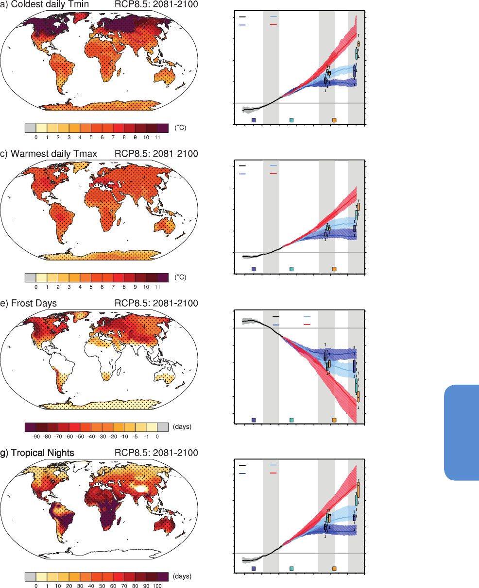
1067

Long-term Climate Change: Projections, Commitments and Irreversibility Chapter 12

Frost Days (FD)

−25

−20

−15

−10

−5

1960 1980 2000 2020 2040 2060 2080 2100

Year

−25

−20

−15

−10

−5

(days)

Warmest daily Tmax (TXx)

1960 1980 2000 2020 2040 2060 2080 2100

Year

−2

(

−2

historical

RCP2.6

RCP4.5

RCP8.5

CMIP3 B1 CMIP3 A1B CMIP3 A2

historical

RCP2.6

RCP4.5

RCP8.5

CMIP3 B1 CMIP3 A1B CMIP3 A2

historical

RCP2.6

RCP4.5

RCP8.5

CMIP3 B1 CMIP3 A1B CMIP3 A2

1960 1980 2000 2020 2040 2060 2080 2100

Year

−2

Coldest daily Tmin (TNn)

(

Tropical Nights (TR)

1960 1980 2000 2020 2040 2060 2080 2100

Year

(days)

historical

RCP2.6

RCP4.5

RCP8.5

CMIP3 B1 CMIP3 A1B CMIP3 A2

Figure 12.13 | CMIP5 multi-model mean geographical changes (relative to a 1981–2000 reference period in common with CMIP3) under RCP8.5 and 20-year smoothed time

series for RCP2.6, RCP4.5 and RCP8.5 in the (a, b) annual minimum of daily minimum temperature, (c, d) annual maximum of daily maximum temperature, (e, f) frost days (number

of days below 0°C) and (g, h) tropical nights (number of days above 20°C). White areas over land indicate regions where the index is not valid. Shading in the time series represents

the interquartile ensemble spread (25th and 75th quantiles). The box-and-whisker plots show the interquartile ensemble spread (box) and outliers (whiskers) for 11 CMIP3 model

simulations of the SRES scenarios A2 (orange), A1B (cyan), and B1 (purple) globally averaged over the respective future time periods (2046–2065 and 2081–2100) as anomalies

from the 1981–2000 reference period. Stippling indicates grid points with changes that are signiﬁcant at the 5% level using a Wilcoxon signed-ranked test. (Updated from Sillmann

et al. (2013), excluding the FGOALS-s2 model.)

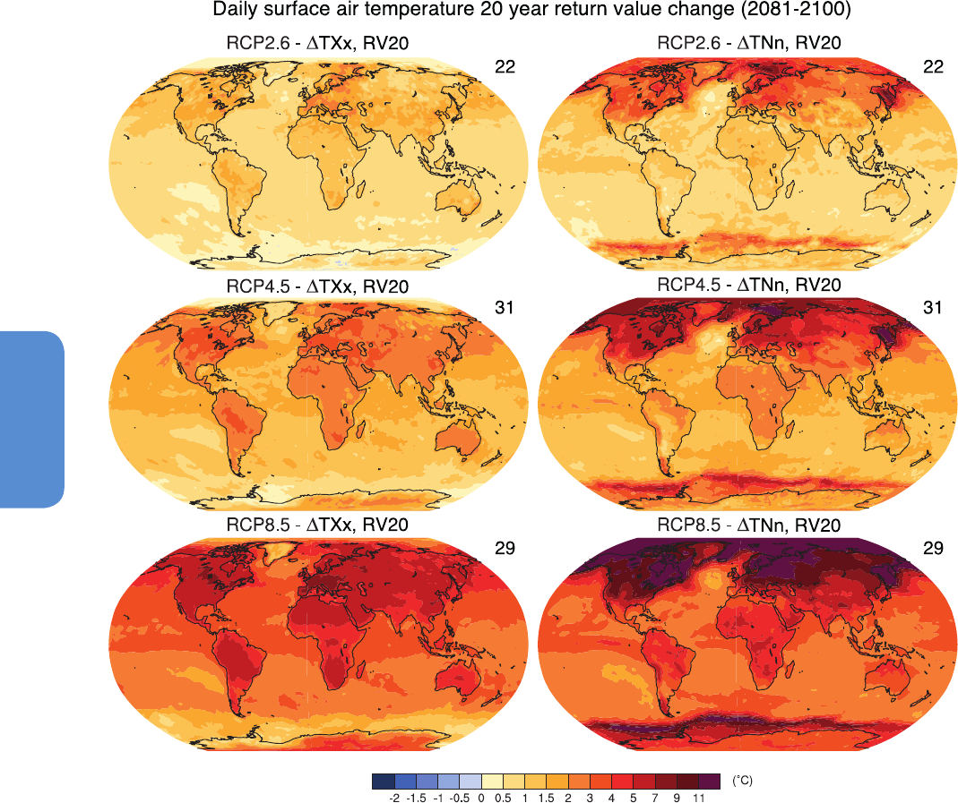
1068

Chapter 12 Long-term Climate Change: Projections, Commitments and Irreversibility

winter mean temperature changes, particularly over parts of North

America and Europe. Kharin et al. (2013) concluded from the CMIP5

models that it is likely that in most land regions a current 20 year max-

imum temperature event is projected to become a one-in-two-year

event by the end of the 21st century under the RCP4.5 and RCP8.5

scenarios, except for some regions of the high latitudes of the NH

where it is likely to become a one-in-ﬁve-year event (see also Senevi-

ratne et al. (2012) Figure 3.5). Current 20-year minimum temperature

events are projected to become exceedingly rare, with return periods

likely increasing to more than 100 years in almost all locations under

RCP8.5 (Kharin et al., 2013). Section 10.6.1.1 notes that a number of

detection and attribution studies since SREX suggest that the model

changes may tend to be too large for warm extremes and too small

for cold extremes and thus these likelihood statements are somewhat

less strongly stated than a direct interpretation of model output and

its ranges. The CMIP5 analysis shown in Figure 12.14 reinforces this

assessment of large changes in the frequency of rare events, particu-

larly in the RCP8.5 scenario (Kharin et al., 2013).

There is high consensus among models in the sign of the future change

in temperature extremes, with recent studies conﬁrming this conclu-

sion from the previous assessments (Tebaldi et al., 2006; Meehl et al.,

2007b; Orlowsky and Seneviratne, 2012; Seneviratne et al., 2012; Sill-

mann et al., 2013). However, the magnitude of the change remains

uncertain owing to scenario and model (both structural and parame-

ter) uncertainty (Clark et al., 2010) as well as internal variability. These

uncertainties are much larger than corresponding uncertainties in the

magnitude of mean temperature change (Barnett et al., 2006; Clark et

al., 2006; Fischer and Schär, 2010; Fischer et al., 2011).

Figure 12.14 | The CMIP5 multi-model median change in 20-year return values of annual warm temperature extremes (left-hand panels) and cold temperature extremes (right-

hand panels) as simulated by CMIP5 models in 2081–2100 relative to 1986–2005 in the RCP2.6 (top), RCP4.5 (middle panels), and RCP8.5 (bottom) experiments.

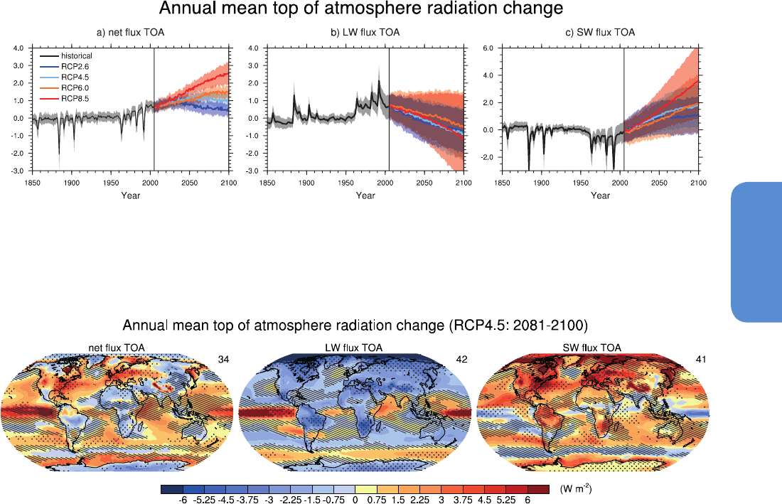
1069

Long-term Climate Change: Projections, Commitments and Irreversibility Chapter 12

12.4.3.4 Energy Budget

Anthropogenic or natural perturbations to the climate system produce

RFs that result in an imbalance in the global energy budget at the

top of the atmosphere (TOA) and affect the global mean temperature

(Section 12.3.3). The climate responds to a change in RF on multiple

time scales and at multiyear time scales the energy imbalance (i.e.,

the energy heating or cooling the Earth) is very close to the ocean

heat uptake due to the much lower thermal inertia of the atmosphere

and the continental surfaces (Levitus et al., 2005; Knutti et al., 2008a;

Murphy et al., 2009; Hansen et al., 2011). The radiative responses of

the ﬂuxes at TOA are generally analysed using the forcing-feedback

framework and are presented in Section 9.7.2.

CMIP5 models simulate a small increase of the energy imbalance at

the TOA over the 20th century (see Box 3.1, Box 9.2 and Box 13.1). The

future evolution of the imbalance is very different depending on the

scenario (Figure 12.15a): for RCP8.5 it continues to increase rapidly,

much less for RCP6.0, it is almost constant for RCP4.5 and decreases

for RCP2.6. This latter negative trend reveals the quasi-stabilization

characteristic of RCP2.6. (In a transient scenario simulation, the TOA

imbalance is always less than the RF because of the slow rate of ocean

heat uptake.)

The rapid ﬂuctuations that are simulated during the 20th century

originate from volcanic eruptions that are prescribed in the models

(see Section 12.3.2). These aerosols reﬂect solar radiation and thus

decrease the amount of SW radiation absorbed by the Earth (Figure

12.15c). The minimum of shortwave (SW) radiation absorbed by the

Earth during the period 1960–2000 is due mainly to two factors: a

sequence of volcanic eruptions and an increase of the reﬂecting aer-

osol burden due to human activities (see Sections 7.5, 8.5 and 9.4.6).

During the 21st century, the absorbed SW radiation monotonically

increases for the RCP8.5 scenario, and increases and subsequently

stabilizes for the other scenarios, consistent with what has been pre-

viously obtained with CMIP3 models and SRES scenarios (Trenberth

and Fasullo, 2009). The two main contributions to the SW changes are

the change of clouds (see Section 12.4.3.5) and the change of the cry-

osphere (see Section 12.4.6) at high latitudes. In the longwave (LW)

domain (Figure 12.15b), the net ﬂux at TOA represents the opposite of

the ﬂux that is emitted by the Earth’s surface and atmosphere toward

space, i.e., a negative anomaly represents an increase of the emitted

(W m

-2

)

Figure 12.15 | Time series of global and annual multi-model mean (a) net total radiation anomaly at the top of the atmosphere (TOA), (b) net longwave radiation anomaly at

the TOA and (c) net shortwave radiation anomaly at the TOA from the CMIP5 concentration-driven experiments for the historical period (black) and the four RCP scenarios. All the

ﬂuxes are positive downward and units are W m

–2

. The anomalies are calculated relative to the 1900–1950 base period as this is a common period to all model experiments with

few volcanic eruptions and relatively small trends. One ensemble member is used for each individual CMIP5 model and the ± standard deviation across the distribution of individual

models is shaded.

Figure 12.16 | Multi-model CMIP5 average changes in annual mean (left) net total radiation anomaly at the top of the atmosphere (TOA), (middle) net longwave radiation

anomaly at the TOA and (right) net shortwave radiation anomaly at the TOA for the RCP4.5 scenario averaged over the periods 2081–2100. All ﬂuxes are positive downward, units

are W m

–2

. The net radiation anomalies are computed with respect to the 1900–1950 base period. Hatching indicates regions where the multi-model mean change is less than one

standard deviation of internal variability. Stippling indicates regions where the multi-model mean change is greater than two standard deviations of internal variability and where

at least 90% of models agree on the sign of change (see Box 12.1).

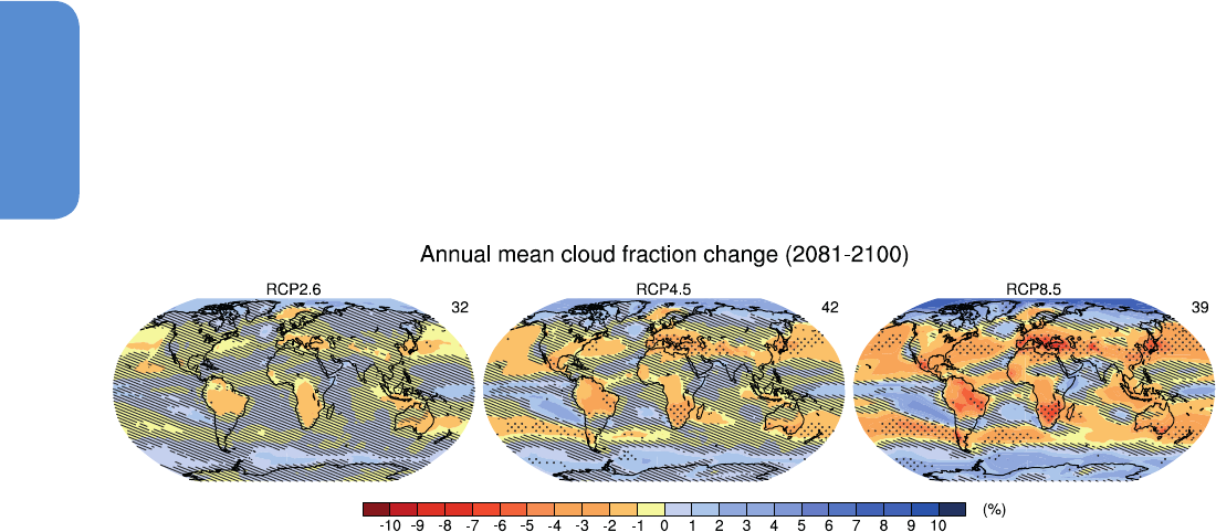
1070

Chapter 12 Long-term Climate Change: Projections, Commitments and Irreversibility

LW radiation. The LW net ﬂux depends mainly on two factors: the sur-

face temperature and the magnitude of the greenhouse effect of the

atmosphere. During the 20th century, the rapid ﬂuctuations of LW radi-

ation are driven by volcanic forcings, which decrease the absorbed SW

radiation, surface temperature, and the LW radiation emitted by the

Earth toward space. During the period 1960–2000, the fast increase of

GHG concentrations also decreases the radiation emitted by the Earth.

In response to this net heating of the Earth, temperatures warm and

thereby increase emitted LW radiation although the change of the tem-

perature vertical proﬁle, water vapour, and cloud properties modulate

this response (e.g., Bony et al., 2006; Randall et al., 2007).

12.4.3.5 Clouds

This section provides a summary description of future changes in

clouds and their feedbacks on climate. A more general and more pre-

cise description and assessment of the role of clouds in the climate

system is provided in Chapter 7, in particular Section 7.2 for cloud pro-

cesses and feedbacks and Section 7.4 for aerosol–cloud interactions.

Cloud feedbacks and adjustments are presented in Section 7.2.5 and a

synthesis is provided in Section 7.2.6. Clouds are a major component

of the climate system and play an important role in climate sensitiv-

ity (Cess et al., 1990; Randall et al., 2007), the diurnal temperature

range (DTR) over land (Zhou et al., 2009), and land–sea contrast (see

Section 12.4.3.1). The observed global mean cloud RF is about –20 W

–2

(Loeb et al., 2009) (see Section 7.2.1), that is, clouds have a net

cooling effect. Current GCMs simulate clouds through various complex

parameterizations (see Section 7.2.3), and cloud feedback is a major

source of the spread of the climate sensitivity estimate (Soden and

Held, 2006; Randall et al., 2007; Dufresne and Bony, 2008) (see Section

9.7.2).

Under future projections the multi-model pattern of total cloud

amount shows consistent decreases in the subtropics, in conjunction

with a decrease of the relative humidity there, and increases at high

latitudes. Another robust pattern is an increase in cloud cover at all

latitudes in the vicinity of the tropopause, a signature of the increase of

the altitude of high level clouds in convective regions (Wetherald and

Manabe, 1988; Meehl et al., 2007b; Soden and Vecchi, 2011; Zelinka

et al., 2012). Low-level clouds were identiﬁed as a primary cause of

inter-model spread in cloud feedbacks in CMIP3 models (Bony and

Dufresne, 2005; Webb et al., 2006; Wyant et al., 2006). Since AR4, these

results have been conﬁrmed along with the positive feedbacks due to

high level clouds in the CMIP3 or CFMIP models (Zelinka and Hart-

mann, 2010; Soden and Vecchi, 2011; Webb et al., 2013) and CMIP5

models (Vial et al., 2013). Since AR4, the response of clouds has been

partitioned in a direct or ‘rapid’ response of clouds to CO

and a ‘slow’

response of clouds to the surface temperature increase (i.e., the usual

feedback response) (Gregory and Webb, 2008). The radiative effect of

clouds depends mainly on their fraction, optical depth and temper-

ature. The contribution of these variables to the cloud feedback has

been quantiﬁed for the multi-model CMIP3 (Soden and Vecchi, 2011)

and CFMIP1 database (Zelinka et al., 2012). These ﬁndings are con-

sistent with the radiative changes obtained with the CMIP5 models

(Figure 12.16) and may be summarized as follows (see Section 7.2.5

for more details).

The dominant contributor to the SW cloud feedback is the change in

cloud fraction. The reduction of cloud fraction between 50°S and 50°N,

except along the equator and the eastern part of the ocean basins

(Figure 12.17), contributes to an increase in the absorbed solar radi-

ation (Figure 12.16c). Physical mechanisms and the role of different

parameterizations have been proposed to explain this reduction of

low-level clouds (Zhang and Bretherton, 2008; Caldwell and Breth-

erton, 2009; Brient and Bony, 2013; Webb et al., 2013). Poleward of

50°S, the cloud fraction and the cloud optical depth increases, thereby

increasing cloud reﬂectance. This leads to a decrease of solar absorp-

tion around Antarctica where the ocean is nearly ice free in summer

(Figure 12.16c). However, there is low conﬁdence in this result because

GCMs do not reproduce the nearly 100% cloud cover observed there

and the negative feedback could be overestimated (Trenberth and

Fasullo, 2010) or, at the opposite, underestimated because the cloud

optical depth simulated by models is biased high there (Zelinka et al.,

2012).

In the LW domain, the tropical high cloud changes exert the dominant

effect. A lifting of the cloud top with warming is simulated consistently

across models (Meehl et al., 2007b) which leads to a positive feed-

back whereby the LW emissions from high clouds decrease as they

cool (Figure 12.16b). The dominant driver of this effect is the increase

of tropopause height and physical explanations have been proposed

(Hartmann and Larson, 2002; Lorenz and DeWeaver, 2007; Zelinka

Figure 12.17 | CMIP5 multi-model changes in annual mean total cloud fraction (in %) relative to 1986–2005 for 2081–2100 under the RCP2.6 (left), RCP4.5 (centre) and RCP8.5

(right) forcing scenarios. Hatching indicates regions where the multi-model mean change is less than one standard deviation of internal variability. Stippling indicates regions where

the multi-model mean change is greater than two standard deviations of internal variability and where 90% of the models agree on the sign of change (see Box 12.1). The number

of CMIP5 models used is indicated in the upper right corner of each panel.

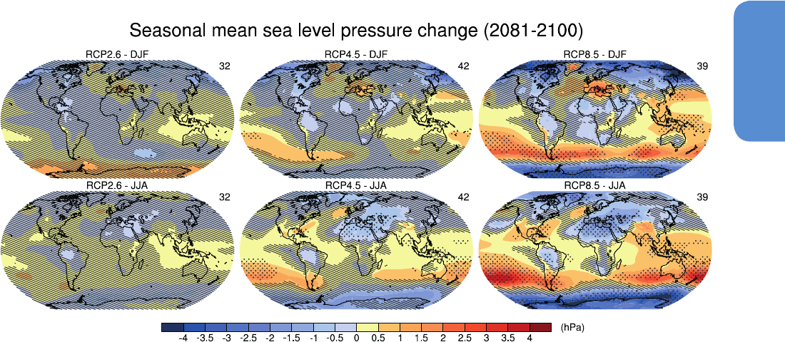
1071

Long-term Climate Change: Projections, Commitments and Irreversibility Chapter 12

and Hartmann, 2010). Although the decrease in cloudiness generally

increases outgoing longwave radiation and partly offsets the effect of

cloud rising, the net effect is a consistent positive global mean LW

cloud feedback across CMIP and CFMIP models. Global mean SW cloud

feedbacks range from slightly negative to strongly positive (Soden and

Vecchi, 2011; Zelinka et al., 2012), with an inter-model spread in net

cloud feedback being mainly attributable to low-level cloud changes.

In summary, both the multi-model mean and the inter-model spread of

the cloud fraction and radiative ﬂux changes simulated by the CMIP5

models are consistent with those previously obtained by the CMIP3

models. These include decreases in cloud amount in the subtropics,

increases at high latitudes and increases in the altitude of high level

clouds in convective regions. Many of these changes have been under-

stood primarily as responses to large-scale circulation changes (see

Section 7.2.6).

12.4.4 Changes in Atmospheric Circulation

Projected changes in energy and water cycles couple with changes in

atmospheric circulation and mass distribution. Understanding this cou-

pling is necessary to assess physical behaviour underlying projected

changes, particularly at regional scales, revealing why changes occur

and the realism of the changes. The focus in this section is on atmos-

pheric circulation behaviour that CMIP5 GCMs resolve well. Thus, the

section includes discussion of extratropical cyclones but not tropical

cyclones: extratropical cyclones are fairly well resolved by most CMIP5

GCMs, whereas tropical cyclones are not, requiring resolutions ﬁner

than used by the large majority of CMIP5 GCMs (see Section 9.5.4.3).

Detailed discussion of tropical cyclones appears in Section 14.6.1

(see also Section 11.3.2.5.3 for near term changes and Section 3.4.4

in Seneviratne et al. (2012)). Regional detail concerning extratropical

storm tracks, including causal processes, appears in Section 14.6.2

(see also Section 11.3.2.4 for near-term changes and Seneviratne et al.

(2012) for an assessment of projected changes related to weather and

climate extremes).

12.4.4.1 Mean Sea Level Pressure and Upper-Air Winds

Sea level pressure gives an indication of surface changes in atmos-

pheric circulation (Figure 12.18). As in previous assessments, a robust

feature of the pattern of change is a decrease in high latitudes and

increases in the mid-latitudes, associated with poleward shifts in the

SH mid-latitude storm tracks (Section 12.4.4.3) and positive trends

in the annular modes (Section 14.5) as well as an expansion of the

Hadley Cell (Section 12.4.4.2). Similar patterns of sea level pressure

change are found in observed trends over recent decades, suggest-

ing an already detectable change (Gillett and Stott, 2009; Section

10.3.3.4), although the observed patterns are inﬂuenced by both natu-

ral and anthropogenic forcing as well as internal variability and the

relative importance of these inﬂuences is likely to change in the future.

Internal variability has been found to play a large role in uncertainties

of future sea level pressure projections, particularly at higher latitudes

(Deser et al., 2012a).

In boreal winter, decreases of sea level pressure over NH high lati-

tudes are slightly weaker in the CMIP5 ensemble compared to previous

assessments, consistent with Scaife et al. (2012) and Karpechko and

Manzini (2012), who suggest that improvements in the representation

of the stratosphere can inﬂuence this pattern. In austral summer, the

SH projections are impacted by the additional inﬂuence of stratospher-

ic ozone recovery (see Section 11.3.2.4.2) which opposes changes due

to GHGs. Under the weaker GHG emissions of RCP2.6, decreases in sea

level pressure over the SH mid-latitudes and increases over SH high

latitudes are consistent with expected changes from ozone recovery

(Arblaster et al., 2011; McLandress et al., 2011; Polvani et al., 2011). For

Figure 12.18 | CMIP5 multi-model ensemble average of December, January and February (DJF, top row) and June, July and August (JJA, bottom row) mean sea level pressure

change (2081–2100 minus 1986–2005) for, from left to right, RCP2.6, 4.5 and 8.5. Hatching indicates regions where the multi-model mean change is less than one standard

deviation of internal variability. Stippling indicates regions where the multi-model mean change is greater than two standard deviations of internal variability and where at least

90% of models agree on the sign of change (see Box 12.1).

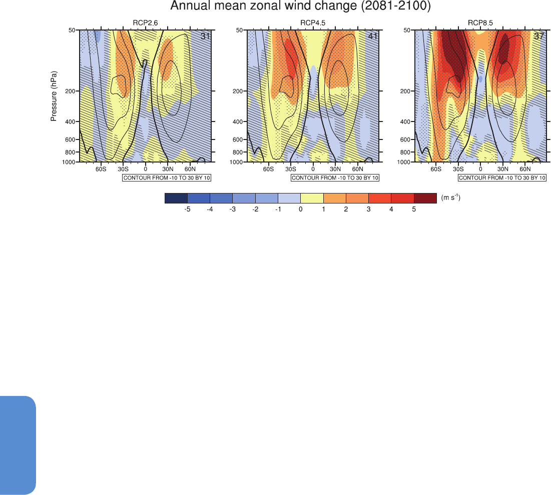
1072

Chapter 12 Long-term Climate Change: Projections, Commitments and Irreversibility

all other RCPs, the magnitude of SH extratropical changes scales with

the RF, as found in previous model ensembles (Paeth and Pollinger,

2010; Simpkins and Karpechko, 2012).

Large increases in seasonal sea level pressure are also found in regions

of sub-tropical drying such as the Mediterranean and northern Africa

in DJF and Australia in JJA. Projected changes in the tropics are less

consistent across the models; however, a decrease in the eastern equa-

torial Paciﬁc and increase over the maritime continent, associated with

a weakening of the Walker Circulation (Vecchi and Soden, 2007; Power

and Kociuba, 2011b), is found in all RCPs.

Future changes in zonal and annual mean zonal winds (Figure 12.19)

are seen throughout the atmosphere with stronger changes in higher

RCPs. Large increases in winds are evident in the tropical stratosphere

and a poleward shift and intensiﬁcation of the SH tropospheric jet is

seen under RCP4.5 and RCP8.5, associated with an increase in the

SH upper tropospheric meridional temperature gradient (Figure 12.12)

(Wilcox et al., 2012). In the NH, the response of the tropospheric jet

is weaker and complicated by the additional thermal forcing of polar

ampliﬁcation (Woollings, 2008). Barnes and Polvani (2013) evaluate

changes in the annual mean mid-latitude jets in the CMIP5 ensemble,

ﬁnding consistent poleward shifts in both hemispheres under RCP8.5

for the end of the 21st century. In the NH, the poleward shift is ~1°,

similar to that found for the CMIP3 ensemble (Woollings and Black-

burn, 2012). In the SH, the annual mean mid-latitude jet shifts pole-

ward by ~2° under RCP8.5 at the end of the 21st century in the CMIP5

multi-model mean (Barnes and Polvani, 2013), with a similar shift of

1.5° in the surface westerlies (Swart and Fyfe, 2012). A strengthen-

ing of the SH surface westerlies is also found under all RCPs except

RCP2.6 (Swart and Fyfe, 2012), with largest changes in the Paciﬁc

basin (Bracegirdle et al., 2013). In austral summer, ozone recovery off-

sets changes in GHGs to some extent, with a weak reversal of the jet

shift found in the multi-model mean under the low emissions scenario

of RCP2.6 (Swart and Fyfe, 2012) and weak or poleward shifts in other

RCPs (Swart and Fyfe, 2012; Wilcox et al., 2012). Eyring et al. (2013)

note the sensitivity of the CMIP5 SH summertime circulation changes

to both the strength of the ozone recovery (simulated by some models

interactively) and the rate of GHG increases.

Although the poleward shift of the tropospheric jets are robust across

models and likely under increased GHGs, the dynamical mechanisms

behind these projections are still not completely understood and have

been explored in both simple and complex models (Chen et al., 2008;

Lim and Simmonds, 2009; Butler et al., 2010). The shifts are associated

with a strengthening in the upper tropospheric meridional temperature

gradient (Wilcox et al., 2012) and hypotheses for associated changes

in planetary wave activity and/or synoptic eddy characteristics that

impact on the position of the jet have been put forward (Gerber et

al., 2012). Equatorward biases in the position of the SH jet (Section

9.5.3.2), while somewhat improved over similar biases in the CMIP3

models (Kidston and Gerber, 2010) still remain, limiting our conﬁdence

in the magnitude of future changes.

In summary, poleward shifts in the mid-latitude jets of about 1 to 2

degrees latitude are likely at the end of the 21st century under RCP8.5

in both hemispheres (medium conﬁdence) with weaker shifts in the NH

and under lower emission scenarios. Ozone recovery will likely weaken

the GHG-induced changes in the SH extratropical circulation in austral

summer.

12.4.4.2 Planetary-Scale Overturning Circulations

Large-scale atmospheric overturning circulations and their interaction

with other atmospheric mechanisms are signiﬁcant in determining trop-

ical climate and regional changes in response to enhanced RF. Observed

Figure 12.19 | Coupled Model Intercomparison Project Phase 5 (CMIP5) multi-model ensemble average of zonal and annual mean wind change (2081–2100 minus 1986–2005)

for, from left to right, Representative Concentration Pathway 2.6 (RCP2.6), 4.5 and 8.5. Black contours represent the multi-model average for the 1986–2005 base period. Hatching

indicates regions where the multi-model mean change is less than one standard deviation of internal variability. Stippling indicates regions where the multi-model mean change is

greater than two standard deviations of internal variability and where at least 90% of models agree on the sign of change (see Box 12.1).

1073

Long-term Climate Change: Projections, Commitments and Irreversibility Chapter 12

changes in tropical atmospheric circulation are assessed in Section 2.7.5,

while Section 10.3.3 discusses attribution of these observed changes to

anthropogenic forcing. Evidence is inconclusive on recent trends in the

strength of the Hadley (Stachnik and Schumacher, 2011) and Walker

Circulations (Vecchi et al., 2006; Sohn and Park, 2010; Merriﬁeld, 2011;

Luo et al., 2012; Tokinaga et al., 2012), though there is medium conﬁ-

dence of an anthropogenic inﬂuence on the observed widening of the

Hadley Circulation (Hu and Fu, 2007; Johanson and Fu, 2009; Davis and

Rosenlof, 2012). In the projections, there are indications of a weakening

of tropical overturning of air as the climate warms (Held and Soden,

2006; Vecchi and Soden, 2007; Gastineau et al., 2008, 2009; Chou and

Chen, 2010; Chadwick et al., 2012; Bony et al., 2013). In the SRES A1B

scenario, CMIP3 models show a remarkable agreement in simulating a

weakening of the tropical atmospheric overturning circulation (Vecchi

and Soden, 2007). CMIP5 models also show a consistent weakening

(Chadwick et al., 2012). Along the ascending branches of tropical over-

turning cells, a reduction in convective mass ﬂux from the boundary

layer to the free atmosphere is implied by the differential response to

global warming of the boundary-layer moisture content and surface

evaporation. This weakening of vertical motion along the ascending

regions of both the tropical meridional and near-equatorial zonal cells

is associated with an imbalance in the rate of atmospheric moisture

increase and that of global mean precipitation (Held and Soden, 2006).

A reduction in the compensating climatological subsidence along the

downward branches of overturning circulations, where the rate of

increase of static stability exceeds radiative cooling, is implied.

Several mechanisms have been suggested for the changes in the inten-

sity of the tropical overturning circulation. The weakening of low-level

convective mass ﬂux along ascending regions of tropical overturning

cells has been ascribed to changes in the hydrologic cycle (Held and

Soden, 2006; Vecchi and Soden, 2007). Advection of dry air from sub-

sidence regions towards the ascending branches of large-scale tropical

circulation has been suggested to be a feasible mechanism weakening

ascent along the edges of convection regions (Chou et al., 2009). A

deepening of the tropical troposphere in response to global warming

increases the vertical extent of convection, which has been shown to

increase the atmosphere’s moist stability and thus also weakening

overturning cells (Chou and Chen, 2010). An imbalance between the

increase in diabatic heating of the troposphere and in static stabili-

ty whereby the latter increases more rapidly has also been thought

to play a role in weakening tropical ascent (Lu et al., 2008). Mean

advection of enhanced vertical stratiﬁcation under GHG forcing which

involves cooling of convective regions and warming of subsidence

regions has been shown to slow down tropical cells (Ma et al., 2012).

The latest ﬁndings using CMIP5 models reveal that an increase in

GHGs ( particularly CO

) contributes signiﬁcantly to weakening tropi-

cal overturning cells by reducing radiative cooling in the upper atmos-

phere (Bony et al., 2013). SST gradients have also been found to play

a role in altering the strength of tropical cells (Tokinaga et al., 2012;

Ma and Xie, 2013). Evidence has been provided suggesting that the SH

Hadley Cell may strengthen in response to meridional SST gradients

featuring reduced warming in the SH subtropical oceans relative to the

NH, particularly over the Paciﬁc and Indian Oceans (Ma and Xie, 2013).

The north-to-south SST warming gradients are a source of intermodel

differences in their projections of changes in the SH Hadley Circulation.

Apart from changes in Hadley Circulation strength, a robust feature

in 21st century climate model simulations is an increase in the cell’s

depth and width (Mitas and Clement, 2006; Frierson et al., 2007; Lu

et al., 2007; Lu et al., 2008), with the latter change translating to a

broadening of tropical regions (Seidel and Randel, 2007; Seidel et al.,

2008) and a poleward displacement of subtropical dry zones (Lu et

al., 2007; Scheff and Frierson, 2012). The increase in the cell’s depth

is consistent with a tropical tropopause rise. The projected increase in

the height of the tropical tropopause and the associated increase in

meridional temperature gradients close to the tropopause slope have

been proposed to be an important mechanism behind the Hadley cell

expansion and the poleward displacement of the subtropical westerly

jet (Lu et al., 2008; Johanson and Fu, 2009). An increase in subtropical

and mid-latitude static stability has been found to be an important

factor widening the Hadley Cell by shifting baroclinic eddy activity and

the associated eddy-driven jet and subsidence poleward (Mitas and

Clement, 2006; Lu et al., 2008). The projected widening of the Hadley

Cell is consistent with late 20th century observations, where ~2° to 5°

latitude expansion was found (Fu et al., 2006; Johanson and Fu, 2009).

The consistency of simulated changes in CMIP3 and CMIP5 models and

the consistency of Hadley Cell changes with the projected tropopause

rise and increase in subtropical and mid-latitude static stability indi-

cate that a widening and weakening of the NH Hadley Cell by the late

21st century is likely.

The zonally asymmetric Walker Circulation is projected to weaken

under global warming (Power and Kociuba, 2011a, 2011b), more than

the Hadley Circulation (Lu et al., 2007; Vecchi and Soden, 2007). The

consistency of the projected Walker Circulation slowdown from CMIP3

to CMIP5 suggests that its change is robust (Ma and Xie, 2013). Almost

everywhere around the equatorial belt, changes in the 500 hPa ver-

tical motion oppose the climatological background motion, notably

over the maritime continent (Vecchi and Soden, 2007; Shongwe et al.,

2011). Around the Indo-Paciﬁc warm pool, in response to a spatially

uniform SST warming, the climatological upper tropospheric diver-

gence weakens (Ma and Xie, 2013). Changes in the strength of the

Walker Circulation also appear to be linked to differential warming

between the Indian and Paciﬁc Ocean warming at low latitudes (Luo et

al., 2012). Over the equatorial Paciﬁc Ocean, where mid-tropospheric

ascent is projected to strengthen, changes in zonal SST and hence sea

level pressure gradients induce low-level westerly wind anomalies that

act to weaken the low-level branch of the Paciﬁc Walker Circulation.

These projected changes in the tropical Paciﬁc circulation are already

occurring (Zhang and Song, 2006). However, the projected weakening

of the Paciﬁc Walker Cell does not imply an increase in the frequency

and/or magnitude of El Niño events (Collins et al., 2010). The consisten-

cy of simulated changes in CMIP3 and CMIP5 models and the consist-

ency of Walker Cell changes with equatorial SST and pressure-gradient

changes that are already observed indicate that a weakening of the

Walker Cell by the late 21st century is likely.

In the upper atmosphere, a robust feature of projected stratospheric

circulation change is that the Brewer–Dobson circulation will likely

strengthen in the 21st century (Butchart et al., 2006, 2010; Li et al.,

2008; McLandress and Shepherd, 2009; Shepherd and McLandress,

2011). In a majority of model experiments, the projected changes in

the large-scale overturning circulation in the stratosphere feature an

1074

Chapter 12 Long-term Climate Change: Projections, Commitments and Irreversibility

intensiﬁcation of tropical upward mass ﬂux, which may extend to the

upper stratosphere. The proposed driver of the increase in mass ﬂux at

the tropical lower stratosphere is the enhanced propagation of wave

activity, mainly resolved planetary waves, associated with a positive

trend in zonal wind structure (Butchart and Scaife, 2001; Garcia and

Randel, 2008). In the 21st century, increases in wave excitation from

diabatic heating in the upper tropical troposphere could reinforce the

wave forcing on the tropical upwelling branch of the stratospheric

mean meridional circulation (Calvo and Garcia, 2009). Parameterized

orographic gravity waves that result from strengthening of subtropical

westerly jets and cause more waves to propagate into the lower strat-

osphere also play a role (Sigmond et al., 2004; Butchart et al., 2006).

The projected intensiﬁcation in tropical upwelling is counteracted by

enhanced mean extratropical/polar lower stratospheric subsidence. In

the NH high latitudes, the enhanced downwelling is associated with an

increase in stationary planetary wave activities (McLandress and Shep-

herd, 2009). The intensiﬁcation of the stratospheric meridional residual

circulation has already been reported in studies focussing on the last

decades of the 20th century (Garcia and Randel, 2008; Li et al., 2008;

Young et al., 2012). The projected increase in troposphere-to-strato-

sphere mass exchange rate (Butchart et al., 2006) and stratospheric

mixing associated with the strengthening of the Brewer–Dobson circu-

lation will likely result in a decrease in the mean age of air in the lower

stratosphere. In the mid-latitude lower stratosphere, quasi-horizontal

mixing is a signiﬁcant contributor to reducing the lifetimes of air. There

are some suggestions that the changes in stratospheric overturning

circulation could lead to a reduction in tropical ozone concentrations

and an increase at high latitudes (Jiang et al., 2007) and an increase

in the amplitude of the annual cycle of stratospheric ozone (Randel et

al., 2007).

12.4.4.3 Extratropical Storms: Tracks and Inﬂuences on

Planetary-Scale Circulation and Transports

Since the AR4, there has been continued evaluation of changes in

extratropical storm tracks under projected warming using both CMIP3

and, more recently, CMIP5 simulations, as well as supporting studies

using single models or idealized simulations. CMIP3 analyses use a

variety of methods for diagnosing storm tracks, but diagnosis of chang-

es in the tracks appears to be relatively insensitive to methods used

(Ulbrich et al., 2013). Analyses of SH storm tracks generally agree with

earlier studies, showing that extratropical storm tracks will tend to

shift poleward (Bengtsson et al., 2009; Gastineau et al., 2009; Gastin-

eau and Soden, 2009; Perrie et al., 2010; Schuenemann and Cassano,

2010; Chang et al., 2012b). The behaviour is consistent with a likely

trend in observed storm-track behaviour (see Section 2.7.6). Similar

behaviour appears in CMIP5 simulations for the SH (Figure 12.20c, d).

In SH winter there is a clear poleward shift in storm tracks of several

degrees and a reduction in storm frequency of only a few percent (not

shown). The poleward shift at the end of the century is consistent with

a poleward shift in the SH of the latitudes with strongest tropospheric

jets (Figure 12.19). This appears to coincide with shifts in baroclinic

dynamics governing extratropical storms (Frederiksen et al., 2011),

though the degree of jet shift appears to be sensitive to bias in a mod-

el’s contemporary-climate storm tracks (Chang et al., 2012a, 2012b).

Although there is thus some uncertainty in the degree of shift, the

consistency of behaviour with observation-based trends, consistency

between CMIP5 and CMIP3 projections under a variety of diagnostics

and the physical consistency of the storm response with other climatic

changes gives high conﬁdence that a poleward shift of several degrees

in SH storm tracks is likely by the end of the 21st century under the

RCP8.5 scenario.

In the NH winter (Figure 12.20a, b), the CMIP5 multi-model ensemble

shows an overall reduced frequency of storms and less indication of

a poleward shift in the tracks. The clearest poleward shift in the NH

winter at the end of the 21st century occurs in the Asia-Paciﬁc storm

track, where intensiﬁcation of the westerly jet promotes more intense

cyclones in an ensemble of CMIP5 models (Mizuta, 2012). Otherwise,

changes in winter storm-track magnitude, as measured by band-pass

sea level pressure ﬂuctuations, show only small change relative to

interannual and inter-decadal variability by the end of the 21st century

in SRES A1B and RCP4.5 simulations for several land areas over the NH

(Harvey et al., 2012). Consistency in CMIP3 and CMIP5 changes seen

in the SH are absent in the NH (Chang et al., 2012a). Factors identiﬁed

that affect changes in the North Atlantic basin’s storm track include

horizontal resolution (Colle et al., 2013) and how models simulate

changes in the Atlantic’s meridional overturning circulation (Catto et

al., 2011; Woollings et al., 2012), the zonal jet and Hadley Circulation

(Mizuta, 2012; Zappa et al., 2013) and subtropical upper troposphere

temperature (Haarsma et al., 2013). Substantial uncertainty and thus

low conﬁdence remains in projecting changes in NH winter storm

tracks, especially for the North Atlantic basin.

Additional analyses of CMIP3 GCMs have determined other changes in

properties of extratropical storms. Most analyses ﬁnd that the frequen-

cy of storms decreases in projected climates (Finnis et al., 2007; Favre

and Gershunov, 2009; Dowdy et al., 2013), though the occurrence of

strong storms may increase in some regions (Pinto et al., 2007; Bengts-

son et al., 2009; Ulbrich et al., 2009; Zappa et al., 2013). Many studies

focus on behaviour of speciﬁc regions, and results of these studies are

detailed in Section 14.6.2.

Changes in extratropical storms in turn may inﬂuence other large-scale

climatic changes. Kug et al. (2010) in a set of time-slice simulations

show that a poleward shift of storm tracks in the NH could enhance

polar warming and moistening. The Arctic Oscillation (AO) is sensitive

to synoptic eddy vorticity ﬂux, so that projected changes in storm

tracks can alter the AO (Choi et al., 2010). The net result is that chang-

es in extratropical storms alter the climate in which they are embed-

ded, so that links between surface warming, extratropical storms and

their inﬂuence on climate are more complex than simple responses to

changes in baroclinicity (O’Gorman, 2010).

12.4.5 Changes in the Water Cycle

The water cycle consists of water stored on the Earth in all its phases,

along with the movement of water through the Earth’s climate system.

In the atmosphere, water occurs primarily as gaseous water vapour,

but it also occurs as solid ice and liquid water in clouds. The ocean is

primarily liquid water, but is partly covered by ice in polar regions. Ter-

restrial water in liquid form appears as surface water (lakes, rivers), soil

moisture and groundwater. Solid terrestrial water occurs in ice sheets,

glaciers, frozen lakes, snow and ice on the surface and permafrost.

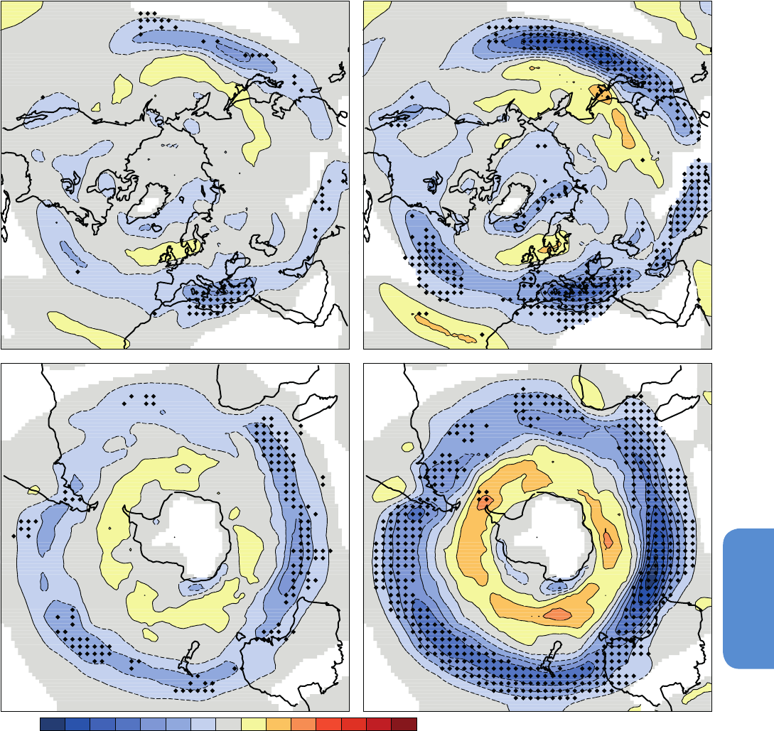
1075

Long-term Climate Change: Projections, Commitments and Irreversibility Chapter 12

RCP4.5: 2081-2100

Southern Hemisphere JJANorthern Hemisphere DJF

RCP8.5: 2081-2100

-3.9 -3.3 -2.7 -2.1 -1.5 -0.9 -0.3 0.3 0.9 1.5 2.1 2.7 3.3 3.9

(number density per month per unit area)

29 29

Figure 12.20 | Change in winter, extratropical storm track density (2081–2100) – (1986–2005) in CMIP5 multi-model ensembles: (a) RCP4.5 Northern Hemisphere December,

January and February (DJF) and (b) RCP8.5 Northern Hemisphere DJF, (c) RCP4.5 Southern Hemisphere June, July and August (JJA) and (d) RCP8.5 Southern Hemisphere JJA.

Storm-track computation uses the method of Bengtsson et al. (2006, their Figure 13a) applied to 6-hourly 850 hPa vorticity computed from horizontal winds in the CMIP5 archive.

The number of models used appears in the upper right of each panel. DJF panels include data for December 1985 and 2080 and exclude December 2005 and December 2100 for

in-season continuity. Stippling marks locations where at least 90% of the models agree on the sign of the change; note that this criterion differs from that used for many other

ﬁgures in this chapter, due to the small number of models providing sufﬁcient data to estimate internal variability of 20-year means of storm-track statistics. Densities have units

(number density per month per unit area), where the unit area is equivalent to a 5° spherical cap (~10

). Locations where the scenario or contemporary-climate ensemble

average is below 0.5 density units are left white.

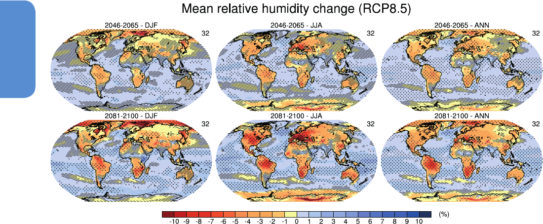
1076

Chapter 12 Long-term Climate Change: Projections, Commitments and Irreversibility

Projections of future changes in the water cycle are inextricably con-

nected to changes in the energy cycle (Section 12.4.3) and atmospheric

circulation (Section 12.4.4).

Saturation vapour pressure increases with temperature, but projected

future changes in the water cycle are far more complex than projected

temperature changes. Some regions of the world will be subject to

decreases in hydrologic activity while others will be subject to increas-

es. There are important local seasonal differences among the responses

of the water cycle to climate change as well.

At ﬁrst sight, the water cycles simulated by CMIP3/5 models may

appear to be inconsistent, particularly at regional scales. Anthropogen-

ic changes to the water cycle are superimposed on complex naturally

varying modes of the climate (such as El Niño-Southern Oscillation

(ENSO), AO, Paciﬁc Decadal Oscillation (PDO), etc.) aggravating the dif-

ferences between model projections. However, by careful consideration

of the interaction of the water cycle with changes in other aspects of

the climate system, the mechanisms of change are revealed, increasing

conﬁdence in projections.

12.4.5.1 Atmospheric Humidity

Atmospheric water vapour is the primary GHG in the atmosphere. Its

changes affect all parts of the water cycle. However, the amount of

water vapour is dominated by naturally occurring processes and not

signiﬁcantly affected directly by human activities. A common experi-

ence from past modelling studies is that relative humidity (RH) remains

approximately constant on climatological time scales and planetary

space scales, implying a strong constraint by the Clausius–Clapeyron

relationship on how speciﬁc humidity will change. The AR4 stated that

‘a broad-scale, quasi-unchanged RH response [to climate change] is

uncontroversial’ (Randall et al., 2007). However, underlying this fairly

straightforward behaviour are changes in RH that can inﬂuence chang-

es in cloud cover and atmospheric convection (Sherwood, 2010). More

recent analysis provides further detail and insight on RH changes. Anal-

ysis of CMIP3 and CMIP5 models shows near-surface RH decreasing

over most land areas as temperatures increase with the notable excep-

tion of parts of tropical Africa (O’Gorman and Muller, 2010) (Figure

12.21). The prime contributor to these decreases in RH over land is the

larger temperature increases over land than over ocean in the RCP sce-

narios (Joshi et al., 2008; Fasullo, 2010; O’Gorman and Muller, 2010).

The speciﬁc humidity of air originating over more slowly warming

oceans will be governed by saturation temperatures of oceanic air. As

this air moves over land and is warmed, its relative humidity drops as

any further moistening of the air over land is insufﬁcient to maintain

constant RH, a behaviour Sherwood et al. (2010) term a last-satura-

tion-temperature constraint. The RH decrease over most land areas by

the end of the 21st century is consistent with a last-saturation-temper-

ature constraint and with observed behaviour during the ﬁrst decade

of the current century (Section 2.5.5; Simmons et al., 2010). Land–

ocean differences in warming are projected to continue through the

21st century, and although the CMIP5 projected changes are small,

they are consistent with a last-saturation constraint, indicating with

medium conﬁdence that reductions in near-surface RH over many land

areas are likely.

12.4.5.2 Patterns of Projected Average Precipitation Changes

Global mean precipitation changes have been presented in Section

12.4.1.1. The processes that govern large-scale changes in precipita-

tion are presented in Section 7.6, and are used here to interpret the

Figure 12.21 | Projected changes in near-surface relative humidity from the CMIP5 models under RCP8.5 for the December, January and February (DJF, left), June, July and August

(JJA, middle) and annual mean (ANN, right) averages relative to 1986–2005 for the periods 2046–2065 (top row), 2081–2100 (bottom row). The changes are differences in relative

humidity percentage (as opposed to a fractional or relative change). Hatching indicates regions where the multi-model mean change is less than one standard deviation of internal

variability. Stippling indicates regions where the multi-model mean change is greater than two standard deviations of internal variability and where at least 90% of models agree

on the sign of change (see Box 12.1).

1077

Long-term Climate Change: Projections, Commitments and Irreversibility Chapter 12

projected changes in RCP scenarios. Changes in precipitation extremes

are presented in Section 12.4.5.5. Further discussion of regional chang-

es, in particular the monsoon systems, is presented in Chapter 14.

Figure 12.22 shows the CMIP5 multi-model average percentage

change in seasonal mean precipitation in the middle of the 21st

century, at the end of the 21st century and at the end of the 22nd

century for the RCP8.5 scenario relative to the 1986–2005 average.

Precipitation changes for all the scenarios are shown in Annex I Sup-

plementary Material and scale approximately with the global mean

temperature (Section 12.4.2). In many regions, changes in precipitation

exhibit strong seasonal characteristics so that, in regions where the

sign of the precipitation changes varies with the season, the annual

mean values (Figure 12.10) may hide some of these seasonal changes,

resulting in weaker conﬁdence than seasonal mean values (Chou et al.,

2013; Huang et al., 2013).

The patterns of multi-model precipitation changes displayed in Figure

12.22 tend to smooth and decrease the spatial contrast of precip-

itation changes simulated by each model, in particular over regions

where model results disagree. Thus the amplitude of the multi-model

ensemble mean precipitation response signiﬁcantly underestimates

the median amplitude computed from each individual model (Neelin

et al., 2006; Knutti et al., 2010a). The CMIP3/5 multi-model ensemble

precipitation projections must be interpreted in the context of uncer-

tainty. Multi-model projections are not probabilistic statements about

the likelihood of changes. Maps of multi-model projected changes are

smoothly varying but observed changes are and will continue to be

much more granular.

To analyze the patterns of projected precipitation changes, a useful

framework consists in decomposing them into a part that is related to

atmospheric circulation changes and a part that is related mostly to

water vapour changes, referred to as dynamical and thermodynamical

components, respectively. However, the deﬁnition of these two com-

ponents may differ among studies. At the time of the AR4, the robust

changes of the difference between precipitation and evaporation

(P – E) were interpreted as a wet-get-wetter and dry-get-drier type

of response (Mitchell et al., 1987; Chou and Neelin, 2004; Held and

Soden, 2006). The theoretical background, which is more relevant over

oceans than over land, is that the lower-tropospheric water vapour

increase with temperature enhances the moisture transported by

the circulation. This leads to additional moisture convergence within

the convergence zones and to additional moisture divergence in the

descent zones, increasing the contrast in precipitation minus evapo-

ration values between moisture convergence and divergence regions.

A weakening of the tropical overturning circulation (see Section

12.4.4.2) partially opposes this thermodynamic response (Chou and

Neelin, 2004; Held and Soden, 2006; Vecchi and Soden, 2007; Chou

et al., 2009; Seager et al., 2010; Allan, 2012; Bony et al., 2013). At the

regional scale the dynamic response may be larger than the thermo-

dynamic response, and this has been analyzed in more detail since

the AR4 (Chou et al., 2009; Seager et al., 2010; Xie et al., 2010; Muller

and O’Gorman, 2011; Chadwick et al., 2012; Scheff and Frierson, 2012;

Bony et al., 2013; Ma and Xie, 2013). Over continents, this simple wet-

get-wetter and dry-get-drier type of response fails for some important

regions such as the Amazon. At the global scale, the net water vapour

transport from oceans to land increases, and therefore the average P –

E over continents also increases (Liepert and Previdi, 2012).

In the mid and high latitudes, a common feature across generations of

climate models is a simulated increased precipitation. The thermody-

namical component explains most of the projected increase (Emori and

Brown, 2005; Seager et al., 2010). This is consistent with theoretical

explanations assuming ﬁxed atmospheric ﬂow patterns but increased

water vapour in the lower troposphere (Held and Soden, 2006). In addi-

tion to this thermodynamical effect, water transport may be modiﬁed

by the poleward shift of the storm tracks and by the increase of their

intensity (Seager et al., 2010; Wu et al., 2011b), although conﬁdence in

such changes in storm tracks may not be high (see Section 12.4.4). On

seasonal time scales, the minimum and maximum values of precipita-

tion both increase, with a larger increase of the maximum and there-

fore an increase of the annual precipitation range (Seager et al., 2010;

Chou and Lan, 2012). In particular, the largest changes over northern

Eurasia and North America are projected to occur during winter. At

high latitudes of the NH, the precipitation increase may lead to an

increase of snowfall in the colder regions and a decrease of snowfall

in the warmer regions due to the decreased number of freezing days

(see Section 12.4.6.2).

Most models simulate a large increase of the annual mean precipita-

tion over the equatorial ocean and an equatorward shift of the Inter-

tropical Convergence Zone (ITCZ), in both summer and winter seasons,

that are mainly explained by atmospheric circulation changes (Chou et

al., 2009; Seager et al., 2010; Sobel and Camargo, 2011). The chang-

es of the atmospheric circulation have different origins. Along the

margins of the convection zones, spatial inhomogeneities, including

local convergence feedback or the rate at which air masses from dry

regions tend to ﬂow into the convection zone, can yield a considerable

sensitivity in precipitation response (Chou et al., 2006; Neelin et al.,

2006). Along the equator, atmosphere–ocean interactions yield to a

maximum of SST warming and a large precipitation increase there (Xie

et al., 2010; Ma and Xie, 2013). Model studies with idealized conﬁgu-

rations suggest that tropical precipitation changes should be interpret-

ed as responses to changes of the atmospheric energy budget rather

than responses to changes of SST (Kang and Held, 2012). All of these

atmospheric circulation changes, and therefore precipitation changes,

can differ considerably from model to model. This is the case over both

ocean and land. For instance, the spread of model projections in the

Sahel region, West Africa, is large in both the CMIP3 and CMIP5 mul-

ti-model data base (Roehrig et al., 2013).

In the subtropical dry regions, there is a robust decrease of P – E that

is accounted for by the thermodynamic contribution (Chou and Neelin,

2004; Held and Soden, 2006; Chou et al., 2009; Seager et al., 2010;

Bony et al., 2013). Over ocean, the spatial heterogeneity of temperature

increase impacts the lower-tropospheric water vapour increase, which

impacts both the thermodynamic and the dynamic responses (Xie et

al., 2010; Ma and Xie, 2013). In addition, the pattern of precipitation

changes in dry regions may be different from that of P – E because the

contribution of evaporation changes can be as large (but of opposite

sign) as the moisture transport changes (Chou and Lan, 2012; Scheff

and Frierson, 2012; Bony et al., 2013). This is especially the case over

the subsidence regions during the warm season over land where the

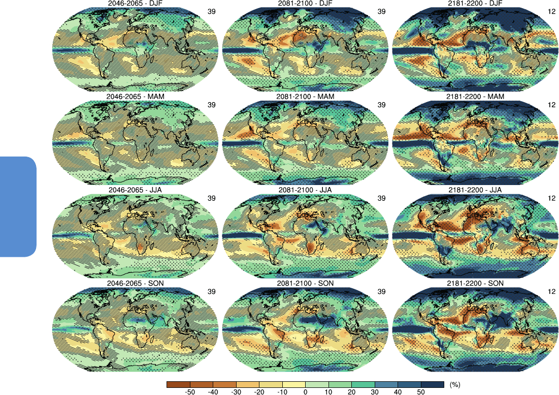
1078

Chapter 12 Long-term Climate Change: Projections, Commitments and Irreversibility

agreement between models is the smallest (Chou et al., 2009; Allan,

2012). A robust feature is the decline of precipitation on the poleward

ﬂanks of the subtropical dry zones as a consequence of the Hadley Cell

expansion, with possible additional decrease from a poleward shift of

the mid latitude storm tracks (Seager et al., 2010; Scheff and Frierson,

2012). On seasonal time scales, the minimum and the maximum values

of precipitation both increase, with a larger increase of the maximum

and therefore an increase of the annual precipitation range (Sobel and

Camargo, 2011; Chou and Lan, 2012).

Long-term precipitation changes are driven mainly by the increase of

the surface temperature, as presented above, but other factors also

contribute to them. Recent studies suggest that CO

increase has a sig-

niﬁcant direct inﬂuence on atmospheric circulation, and therefore on

global and tropical precipitation changes (Andrews et al., 2010; Bala et

al., 2010; Cao et al., 2012; Bony et al., 2013). Over the ocean, the pos-

itive RF from increased atmospheric CO

reduces the radiative cooling

of the troposphere and the large scale rising motion and hence reduc-

es precipitation in the convective regions. Over large landmasses, the

direct effect of CO

on precipitation is the opposite owing to the small

thermal inertia of land surfaces (Andrews et al., 2010; Bala et al., 2010;

Cao et al., 2012; Bony et al., 2013). Regional precipitation changes are

also inﬂuenced by aerosol and ozone (Ramanathan et al., 2001; Allen

et al., 2012; Shindell et al., 2013a) through both local and large-scale

processes, including changes in the circulation. Stratospheric ozone

depletion contributes to the poleward expansion of the Hadley Cell

and the related change of precipitation in the SH (Kang et al., 2011)

whereas black carbon and tropospheric ozone increases are major con-

tributors in the NH (Allen et al., 2012). Regional precipitation changes

depend on regional forcings and on how models simulate their local

and remote effects. Based on CMIP3 results, the inter-model spread

of the estimate of precipitation changes over land is larger than the

inter-scenario spread except in East Asia (Frieler et al., 2012).

Seasonal mean percentage precipitation change (RCP8.5)

Figure 12.22 | Multi-model CMIP5 average percentage change in seasonal mean precipitation relative to the reference period 1986–2005 averaged over the periods 2045–2065,

2081–2100 and 2181–2200 under the RCP8.5 forcing scenario. Hatching indicates regions where the multi-model mean change is less than one standard deviation of internal

variability. Stippling indicates regions where the multi-model mean change is greater than two standard deviations of internal variability and where at least 90% of models agree

on the sign of change (see Box 12.1).

1079

Long-term Climate Change: Projections, Commitments and Irreversibility Chapter 12

Projected precipitation changes vary greatly between models, much

more so than for temperature projections. Part of this variance is due to

genuine differences between the models including their ability to rep-

licate observed precipitation patterns (see Section 9.4.1.1). However, a

large part of it is also the result of the small ensemble size from each

model (Rowell, 2012). This is especially true for regions of small pro-

jected changes located between two regions: one experiencing signif-

icant increases while the other experiences signiﬁcant decreases. Indi-

vidual climate model realizations will differ in their projection of future

precipitation changes in these regions simply owing to their internal

variability (Deser et al., 2012b; Deser et al., 2012a). Multi-model pro-

jections containing large numbers of realizations would tend to feature

small changes in these regions, and hatching in Figure 12.22 indicates

regions where the projected multi-model mean change is less than one

standard deviation of internal variability (method (a), Box 12.1). Conﬁ-

dence in projections in regions of limited or no change in precipitation

may be more difﬁcult to obtain than conﬁdence in regions of large pro-

jected changes. However, Power et al. (2012) and Tebaldi et al. (2011)

show that for some of the regions featuring small multi-model average

projected changes, effective consensus in projections may be better

than the metrics reported in AR4 would imply.

Since the AR4, progress has been made in the understanding of the

processes that control large scale precipitation changes. There is high

conﬁdence that the contrast of seasonal mean precipitation between

dry and wet regions will increase in a warmer climate over most of

the globe although there may be regional exceptions to this general

pattern. This response is particularly robust when considering P – E

changes as a function of atmospheric dynamical regimes. However, it

is important to note that signiﬁcant exceptions can occur in speciﬁc

regions especially along the equator and on the poleward edges of the

subtropical dry zone. In these regions, atmospheric circulation changes

lead to shifts of the precipitation patterns. There is high conﬁdence that

the contrast between wet and dry seasons will increase over most of

the globe as temperatures increase. Over the mid- and high-latitude

regions, projected precipitation increases in winter are larger than in

summer. Over most of the subtropical oceans, projected precipitation

increases in summer are larger than in winter.

The changes in precipitation shown in Figure 12.22 exhibit patterns

that become more pronounced and conﬁdence in them increases

as temperatures increase. More generally, the spatial and temporal

changes in precipitation between two scenarios or within two peri-

ods of a given scenario exhibit the pattern scaling behavior and lim-

itations described in Section 12.4.2. The patterns and the associated

multi-model spreads in CMIP5 for the RCP scenarios are very similar

to those in CMIP3 for the SRES scenarios discussed in the AR4, with

the projections in CMIP5 being slightly more consistent over land than

those from CMIP3 (Knutti and Sedláček, 2013). The largest percentage

changes are at the high latitudes. By the end of the 21st century, over

the large northern land masses, increased precipitation is likely under

the RCP8.5 scenario in the winter and spring poleward of 50°N. The

robustness across scenarios, the magnitude of the projected changes

versus natural variability and physical explanations described above

yield high conﬁdence that the projected changes would be larger than

natural 20-year variations (see Box 12.1). In the tropics, precipitation

changes exhibit strong regional contrasts, with increased precipitation

over the equatorial Paciﬁc and Indian Oceans and decreases over much

of the subtropical ocean. However, decreases are not projected to be

larger than natural 20-year variations anywhere until the end of this

century under the RCP8.5 scenario. Decreased precipitation in the

Mediterranean, Caribbean and Central America, southwestern United

States and South Africa is likely under the RCP8.5 scenario and is pro-

jected with medium conﬁdence to be larger than natural variations by

the end of the 22nd century in some seasons (Box 12.1). The CMIP3

models’ historical simulations of zonal mean precipitation trends were

shown to underestimate observed trends (Gillett et al., 2004; Lambert

et al., 2005; Zhang et al., 2007; Liepert and Previdi, 2009) (see Section

10.3.2.2). Therefore it is more likely than not that the magnitude of the

projected future changes in Figure 12.22 based on the multi-model

mean is underestimated. Observational uncertainties including limited

global coverage and large natural variability, in addition to challenges

in precipitation modelling, limit conﬁdence in assessment of climatic

changes in precipitation.

12.4.5.3 Soil Moisture

Near-surface soil moisture is the net result of a suite of complex process-

es (e.g., precipitation evapotranspiration, drainage, overland ﬂow, inﬁl-

tration), and heterogeneous and difﬁcult-to-characterize aboveground

and belowground system properties (e.g., slope, soil texture). As a

result, regional to global-scale simulations of soil moisture and drought

remain relatively uncertain (Burke and Brown, 2008; Henderson-Sellers

et al., 2008). The AR4 (Section 8.2.3.2) discussed the lack of assess-

ments of global-scale models in their ability to simulate soil moisture,

and this problem appears to have persisted (Section 9.4.4.2). Further-

more, consistent multi-model projections of total soil moisture are difﬁ-

cult to make owing to substantial differences between climate models

in the depth of their soil. However, Koster et al. (2009a) argued that

once climatological statistics affecting soil moisture were accounted for,

different models tend to agree on soil moisture projections.

The AR4 summarized multi-model projections of 21st century annual

mean soil moisture changes as decreasing in the subtropics and Med-

iterranean region, and increasing in east Africa and central Asia. Dai

(2013) found similar changes in an ensemble of 11 CMIP5 GCMs under

RCP4.5. Figure 12.23 shows projected changes in surface soil moisture

(upper 10 cm) in the CMIP5 ensemble at the end of the 21st century

under the RCPs 2.6, 4.5, 6.0 and 8.5. We focus on this new CMIP5

speciﬁcation because it describes soil moisture at a consistent depth

across all CMIP5 models. The broad patterns are moderately consist-

ent across the RCPs, with the changes tending to become stronger as

the strength of the forcing change increases. The agreement among

CMIP5 models and the consistency with other physical features of

climate change indicate high conﬁdence in certain regions where

surface soils are projected to dry. There is little-to-no conﬁdence any-

where in projections of moister surface soils. Under RCP8.5, with the

largest projected change, individual ensemble members (not shown)

show consistency across the ensemble for drying in the Mediterranean

region, northeast and southwest South America, southern Africa, and

southwestern USA. However, ensemble members show disagreement

on the sign of change in large regions such as central Asia or the high

northern latitudes. The Mediterranean, southwestern USA, northeast

South America and southern African drying regions are consistent with

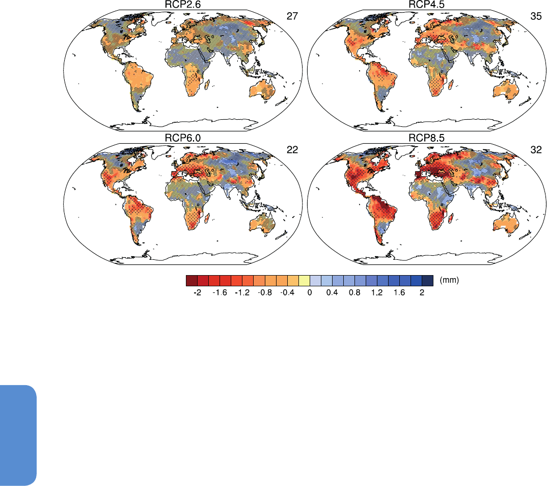
1080

Chapter 12 Long-term Climate Change: Projections, Commitments and Irreversibility

projected widening of the Hadley Circulation that shifts downwelling,

thus inhibiting precipitation in these regions. The large-scale drying in

the Mediterranean, southwest USA, and southern Africa appear across

generations of projections and climate models and is deemed likely

as global temperatures rise and will increase the risk of agricultural

drought. In addition, an analysis of CMIP3 and CMIP5 projections of

soil moisture in ﬁve drought-prone regions indicates that the differ-

ences in future forcing scenarios are the largest source of uncertain-

ty in such regions rather than differences between model responses

(Orlowsky and Seneviratne, 2012).

Other recent assessments include multi-model ensemble approaches,

dynamical downscaling, and regional climate models applied around

the globe and illustrate the variety of issues inﬂuencing soil moisture

changes. Analyses of the southwestern USA using CMIP3 models

(Christensen and Lettenmaier, 2007; Seager et al., 2007) show consist-

ent projections of drying, primarily due to a decrease in winter precipi-

tation. In contrast, Kellomaki et al. (2010) ﬁnd that SRES A2 projections

for Finland yield decreased snow depth, but soil moisture generally

increases, consistent with the general increase in precipitation occur-

ring in high northern latitudes. Kolomyts and Surova (2010), using pro-

jections from the CMIP3 models, GISS and HadCM2, under the SRES

A2 forcing, show that vegetation type has substantial inﬂuence on the

development of pronounced drying over the 21st century in Middle

Volga Region forests.

Projected changes in soil moisture from the CMIP3/5 models also show

substantial seasonal variation. For example, soil moisture changes in

the North American midlatitudes, coupled with projected warming,

increases the strength of land–atmosphere coupling during spring and

summer in 15 GCMs under RCP8.5 (Dirmeyer et al., 2013). For the

Cline River watershed in western Canada, Kienzle et al. (2012) ﬁnd

decreases in summer soil moisture content, but annual increases aver-

aging 2.6% by the 2080s using a suite of CMIP3 GCMs simulating B1,

A1B and A2 scenarios to drive a regional hydrology model. Hansen et

al. (2007), using dynamical downscaling of one GCM running the A2

scenario, ﬁnd summer soil moisture decreases in Mongolia of up to

6% due to increased potential evaporation in a warming climate and

decreased precipitation and decreased precipitation.

Soil moisture projections in high latitude permafrost regions are crit-

ically important for assessing future climate feedbacks from trace-

gas emissions (Zhuang et al., 2004; Riley et al., 2011) and vegetation

changes (Chapin et al., 2005). In addition to changes in precipitation,

snow cover and evapotranspiration, future changes in high-latitude

soil moisture also will depend on permafrost degradation, thermokarst

evolution, rapid changes in drainage (Smith et al., 2005), and changes

in plant communities and their water demands. Current understanding

of these interacting processes at scales relevant to climate is poor, so

that full incorporation in current GCMs is lacking.

Figure 12.23 | Change in annual mean soil moisture (mass of water in all phases in the uppermost 10 cm of the soil) (mm) relative to the reference period 1986–2005 projected

for 2081–2100 from the CMIP5 ensemble. Hatching indicates regions where the multi-model mean change is less than one standard deviation of internal variability. Stippling

indicates regions where the multi-model mean change is greater than two standard deviations of internal variability and where at least 90% of models agree on the sign of change

(see Box 12.1). The number of CMIP5 models used is indicated in the upper right corner of each panel.

Annual mean near-surface soil moisture change (2081-2100)

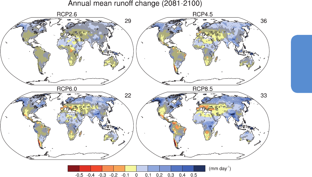
1081

Long-term Climate Change: Projections, Commitments and Irreversibility Chapter 12

12.4.5.4 Runoff and Evaporation

In the AR4, 21st century model-projected runoff consistently showed

decreases in southern Europe, the Middle East, and southwestern USA

and increases in Southeast Asia, tropical East Africa and at high north-

ern latitudes. The same general features appear in the CMIP5 ensemble

of GCMs for all four RCPs shown in Figure 12.24, with the areas of most

robust change typically increasing with magnitude of forcing change.

However, the robustness of runoff decreases in the southwestern USA

is less in the CMIP5 models compared to the AR4. The large decreases

in runoff in southern Europe and southern Africa are consistent with

changes in the Hadley Circulation and related precipitation decreases

and warming-induced evapotranspiration increases. The high northern

latitude runoff increases are likely under RCP8.5 and consistent with

the projected precipitation increases (Figure 12.22). The consistency of

changes across different generations of models and different forcing

scenarios, together with the physical consistency of change indicates

that decreases are also likely in runoff in southern Europe, the Middle

East, and southern Africa in this scenario.

A number of reports since the AR4 have updated ﬁndings from CMIP3

models and analyzed a large set of mechanisms affecting runoff. Sev-

eral studies have focussed on the Colorado River basin in the United

States (Christensen and Lettenmaier, 2007; McCabe and Wolock, 2007;

Barnett and Pierce, 2008; Barnett et al., 2008) showing that runoff

reductions that do happen under global warming occur through a

combination of evapotranspiration increases and precipitation decreas-

es, with the overall reduction in river ﬂow exacerbated by human water

demands on the basin’s supply.

A number of CMIP3 analyses have examined trends and seasonal shifts

in runoff. For example, Kienzle et al. (2012) studied climate change sce-

narios over the Cline River watershed in western Canada and projected

(1) spring runoff and peak streamﬂow up to 4 weeks earlier than in

1961–1990; (2) signiﬁcantly higher streamﬂow between October and

June; and (3) lower streamﬂow between July and September. For the

Mediterranean basin, an ensemble of regional climate models driven

by several GCMs using the A1B scenario have a robust decrease in

runoff emerging only after 2050 (Sanchez-Gomez et al., 2009).

Annual mean surface evaporation in the models assessed in AR4

showed increases over most of the ocean and increases or decreases

over land with largely the same pattern over land as increases and

decreases in precipitation. Similar behaviour occurs in an ensemble of

CMIP5 models (Figure 12.25). Evaporation increases over most of the

ocean and land, with prominent areas of decrease over land occurring

in southern Africa and northwestern Africa along the Mediterranean.

The areas of decrease correspond to areas with reduced precipitation.

There is some uncertainty about storm-track changes over Europe (see

Sections 12.4.3 and 14.6.2). However, the consistency of the decreas-

es across different generations of models and different forcing sce-

narios along with the physical basis for the precipitation decrease

Figure 12.24 | Change in annual mean runoff relative to the reference period 1986–2005 projected for 2081–2100 from the CMIP5 ensemble. Hatching indicates regions where

the multi-model mean change is less than one standard deviation of internal variability. Stippling indicates regions where the multi-model mean change is greater than two standard

deviations of internal variability and where at least 90% of models agree on the sign of change (see Box 12.1). The number of CMIP5 models used is indicated in the upper right

corner of each panel.

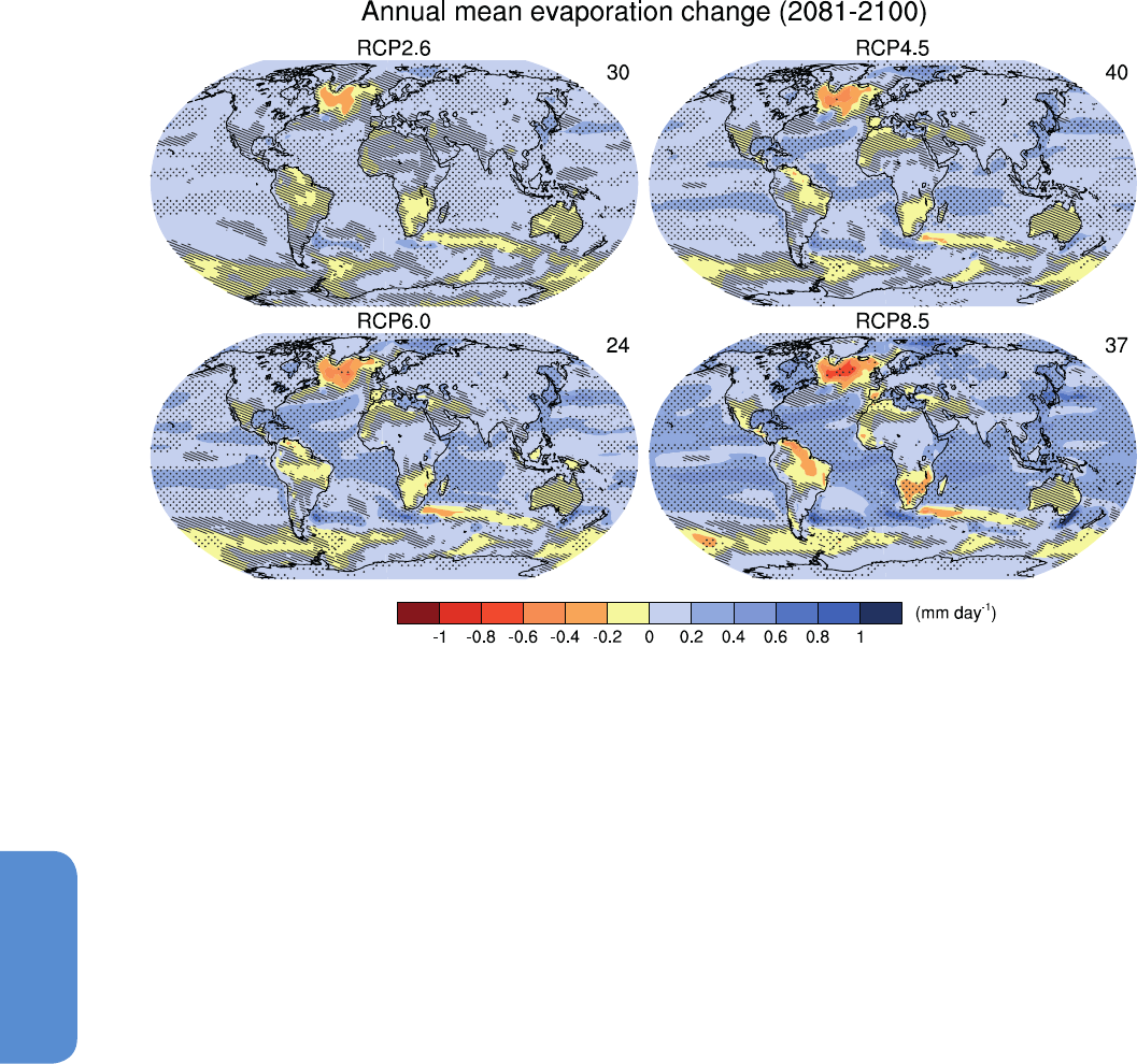
1082

Chapter 12 Long-term Climate Change: Projections, Commitments and Irreversibility

indicates that these decreases in annual mean evaporation are likely

under RCP8.5, but with medium conﬁdence. Annual mean evapora-

tion increases over land in the northern high latitudes are consistent

with the increase in precipitation and the overall warming that would

increase potential evaporation. For the northern high latitudes, the

physical consistency and the similar behaviour across multiple gener-

ations and forcing scenarios indicates that annual mean evaporation

increases there are likely, with high conﬁdence.

Evapotranspiration changes partly reﬂect changes in precipitation.

However, some changes might come from altered biological processes.

For example, increased atmospheric CO

promotes stomatal closure

and reduced transpiration (Betts et al., 2007; Cruz et al., 2010) which

can potentially yield increased runoff. There is potential for substan-

tial feedback between vegetation changes and regional water cycles,

though the impact of such feedback remains uncertain at this point

due to limitations on modelling crop and other vegetation processes in

GCMs (e.g., Newlands et al., 2012) and uncertainties in plant response,

ecosystem shifts and land management changes.

12.4.5.5 Extreme Events in the Water Cycle

In addition to the changes in the seasonal pattern of mean precipitation

described above, the distribution of precipitation events is projected to

undergo profound changes (Gutowski et al., 2007; Sun et al., 2007;

Boberg et al., 2010). At daily to weekly scales, a shift to more intense

individual storms and fewer weak storms is projected (Seneviratne et

al., 2012). At seasonal or longer time scales, increased evapotranspira-

tion over land can lead to more frequent and more intense periods of

agricultural drought.

A general relationship between changes in total precipitation and

extreme precipitation does not exist (Seneviratne et al., 2012). Two

possible mechanisms controlling short-term extreme precipitation

amounts are discussed at length in the literature and are similar to the

thermodynamic and dynamical mechanisms detailed above for chang-

es in average precipitation.

The ﬁrst considers that extreme precipitation events occur when most

of the available atmospheric water vapour rapidly precipitates out in a

single storm. The maximum amount of water vapour in air (saturation)

is determined by the Clausius–Clapeyron relationship. As air temper-

ature increases, this saturated amount of water also increases (Allen

and Ingram, 2002; Pall et al., 2007; Allan and Soden, 2008; Kendon et

al., 2010). Kunkel et al. (2013) examined the CMIP5 model RCP4.5 and

8.5 projections for changes in maximum water vapour concentrations,

a principal factor controlling the probable bound on maximum precipi-

tation, concluding that maximum water vapour changes are compara-

ble to mean water vapour changes but that the potential for changes

in dynamical factors is less compelling. Such increases in atmospheric

water vapour are expected to increase the intensity of individual pre-

cipitation events, but have less impact on their frequency. As a result

Figure 12.25 | Change in annual mean evaporation relative to the reference period 1986–2005 projected for 2081–2100 from the CMIP5 ensemble. Hatching indicates regions

where the multi-model mean change is less than one standard deviation of internal variability. Stippling indicates regions where the multi-model mean change is greater than two

standard deviations of internal variability and where at least 90% of models agree on the sign of change (see Box 12.1). The number of CMIP5 models used is indicated in the

upper right corner of each panel.

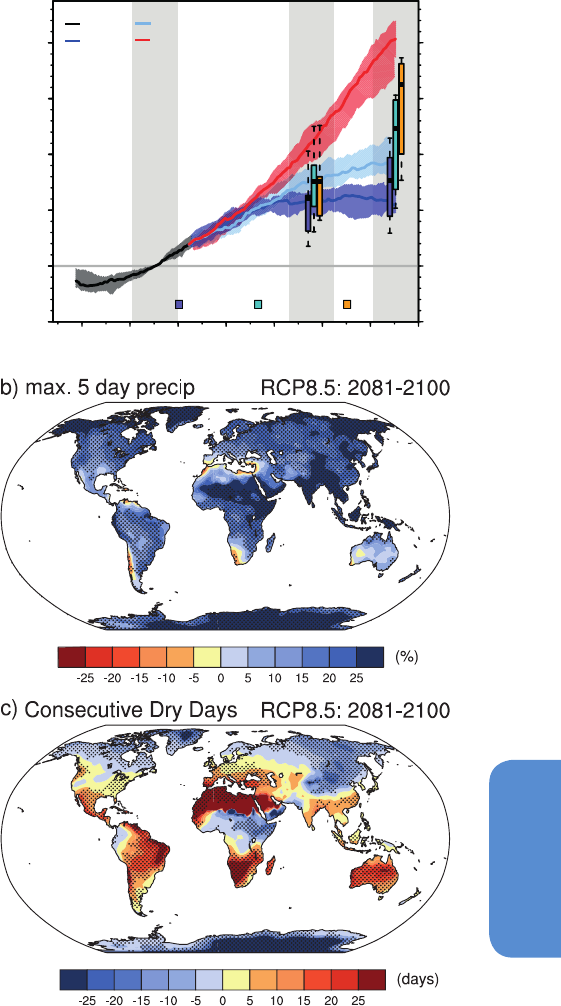
1083

Long-term Climate Change: Projections, Commitments and Irreversibility Chapter 12

projected increases in extreme precipitation may be more reliable than

similar projections of changes in mean precipitation in some regions

(Kendon et al., 2010).

A second mechanism for extreme precipitation put forth by O’Gorman

and Schneider (2009a, 2009b) is that such events are controlled by

anomalous horizontal moisture ﬂux convergence and associated con-

vective updrafts which would change in a more complicated fashion

in a warmer world (Sugiyama et al., 2010). Emori and Brown (2005)

showed that the thermodynamic mechanism dominated over the

dynamical mechanism nearly everywhere outside the tropical warm

pool. However, Utsumi et al. (2011) used gridded observed daily data

to ﬁnd that daily extreme precipitation monotonically increases with

temperature only at high latitudes, with the opposite behaviour in

the tropics and a mix in the mid-latitudes. Li et al. (2011a) found that

both mechanisms contribute to extreme precipitation in a high-res-

olution aquaplanet model with updrafts as the controlling element

in the tropics and air temperature controlling the mid-latitudes con-

sistent with the results by Chou et al. (2012). Using a high-resolution

regional model, Berg et al. (2009) found a seasonal dependence in

Europe with the Clausius–Clapeyron relationship providing an upper

limit to daily precipitation intensity in winter but water availability

rather than storage capacity is the controlling factor in summer. Addi-

tionally, Lenderink and Van Meijgaard (2008) found that very short

(sub-daily) extreme precipitation events increase at a rate twice the

amount predicted by Clausius–Clapeyron scaling in a very high-resolu-

tion model over Europe suggesting that both mechanisms can interact

jointly. Gastineau and Soden (2009) found in the CMIP3 models that

the updrafts associated with the most extreme tropical precipitation

events actually weaken despite an increase in the frequency of the

heaviest rain rates further complicating simple mechanistic explana-

tions. See also Sections 7.6.5 and 11.3.2.5.2.

Projections of changes in future extreme precipitation may be larger

at the regional scales than for future mean precipitation, but natural

variability is also larger causing a tendency for signal-to-noise ratios

to decrease when considering increasingly extreme metrics. However,

mechanisms of natural variability still are a large factor in assessing

the robustness of projections (Kendon et al., 2008). In addition, large-

scale circulation changes, which are uncertain, could dominate over the

above mechanisms depending on the rarity and type of events consid-

ered. However, analysis of CMIP3 models suggests circulation changes

are potentially insufﬁcient to offset the inﬂuence of increasing atmos-

pheric water vapour on extreme precipitation change over Europe at

least on large spatial scales (Kendon et al., 2010). An additional shift of

the storm track has been shown in models with a better representation

of the stratosphere, and this is found to lead to an enhanced increase

in extreme rainfall over Europe in winter (Scaife et al., 2012).

Similar to temperature extremes (Section 12.4.3.3), the deﬁnition of

a precipitation extreme depends very much on context and is often

used in discussion of particular climate-related impacts (Seneviratne

et al. (2012), Box 3.1). Consistently, climate models project future epi-

sodes of more intense precipitation in the wet seasons for most of the

land areas, especially in the NH and its higher latitudes, and the mon-

soon regions of the world, and at a global average scale. The actual

magnitude of the projected change is dependent on the model used,

1960 1980 2000 2020 2040 2060 2080 2100

−5

Year

−5

Wettest consecutive five days (RX5day)

Relative change (%)

historical

RCP2.6

RCP4.5

RCP8.5

CMIP3 B1 CMIP3 A1B CMIP3 A2

Figure 12.26 | (a, b) Projected percent changes (relative to the 1981–2000 refer-

ence period in common with CMIP3) from the CMIP5 models in RX5day, the annual

maximum ﬁve-day precipitation accumulation. (a) Global average percent change over

land regions for the RCP2.6, RCP4.5 and RCP8.5 scenarios. Shading in the time series

represents the interquartile ensemble spread (25th and 75th quantiles). The box-and-

whisker plots show the interquartile ensemble spread (box) and outliers (whiskers) for

11 CMIP3 model simulations of the SRES scenarios A2 (orange), A1B (cyan) and B1

(purple) globally averaged over the respective future time periods (2046–2065 and

2081–2100) as anomalies from the 1981–2000 reference period. (b) Percent change

over the 2081–2100 period in the RCP8.5 scenario. (c) Projected change in annual

CDD, the maximum number of consecutive dry days when precipitation is less than 1

mm, over the 2081–2100 period in the RCP8.5 scenario (relative to the 1981–2000

reference period) from the CMIP5 models. Stippling indicates gridpoints with changes

that are signiﬁcant at the 5% level using a Wilcoxon signed-ranked test. (Updated from

Sillmann et al. (2013), excluding the FGOALS-s2 model.)

1084

Chapter 12 Long-term Climate Change: Projections, Commitments and Irreversibility

Frequently Asked Questions

FAQ 12.2 | How Will the Earth’s Water Cycle Change?

The ﬂow and storage of water in the Earth’s climate system are highly variable, but changes beyond those due to

natural variability are expected by the end of the current century. In a warmer world, there will be net increases in

rainfall, surface evaporation and plant transpiration. However, there will be substantial differences in the changes

between locations. Some places will experience more precipitation and an accumulation of water on land. In others,

the amount of water will decrease, due to regional drying and loss of snow and ice cover.

The water cycle consists of water stored on the Earth in all its phases, along with the movement of water through

the Earth’s climate system. In the atmosphere, water occurs primarily as a gas—water vapour—but it also occurs as

ice and liquid water in clouds. The ocean, of course, is primarily liquid water, but the ocean is also partly covered by

ice in polar regions. Terrestrial water in liquid form appears as surface water—such as lakes and rivers—soil moisture

and groundwater. Solid terrestrial water occurs in ice sheets, glaciers, snow and ice on the surface and in permafrost

and seasonally frozen soil.

Statements about future climate sometimes say that the water cycle will accelerate, but this can be misleading, for

strictly speaking, it implies that the cycling of water will occur more and more quickly with time and at all locations.

Parts of the world will indeed experience intensiﬁcation of the water cycle, with larger transports of water and

more rapid movement of water into and out of storage reservoirs. However, other parts of the climate system will

experience substantial depletion of water, and thus less movement of water. Some stores of water may even vanish.

As the Earth warms, some general features of change will occur simply in response to a warmer climate. Those

changes are governed by the amount of energy that global warming adds to the climate system. Ice in all forms will

melt more rapidly, and be less pervasive. For example, for some simulations assessed in this report, summer Arctic

sea ice disappears before the middle of this century. The atmosphere will have more water vapour, and observations

and model results indicate that it already does. By the end of the 21st century, the average amount of water vapour

in the atmosphere could increase by 5 to 25%, depending on the amount of human emissions of greenhouse gases

and radiatively active particles, such as smoke. Water will evaporate more quickly from the surface. Sea level will

rise due to expansion of warming ocean waters and melting land ice ﬂowing into the ocean (see FAQ 13.2).

These general changes are modiﬁed by the complexity of the climate system, so that they should not be expected

to occur equally in all locations or at the same pace. For example, circulation of water in the atmosphere, on land

and in the ocean can change as climate changes, concentrating water in some locations and depleting it in others.

The changes also may vary throughout the year: some seasons tend to be wetter than others. Thus, model simu-

lations assessed in this report show that winter precipitation in northern Asia may increase by more than 50%,

whereas summer precipitation there is projected to hardly change. Humans also intervene directly in the water

cycle, through water management and changes in land use. Changing population distributions and water practices

would produce further changes in the water cycle.

Water cycle processes can occur over minutes, hours, days and longer, and over distances from metres to kilometres

and greater. Variability on these scales is typically greater than for temperature, so climate changes in precipitation

are harder to discern. Despite this complexity, projections of future climate show changes that are common across

many models and climate forcing scenarios. Similar changes were reported in the AR4. These results collectively

suggest well understood mechanisms of change, even if magnitudes vary with model and forcing. We focus here

on changes over land, where changes in the water cycle have their largest impact on human and natural systems.

Projected climate changes from simulations assessed in this report (shown schematically in FAQ 12.2, Figure 1) gen-

erally show an increase in precipitation in parts of the deep tropics and polar latitudes that could exceed 50% by the

end of the 21st century under the most extreme emissions scenario. In contrast, large areas of the subtropics could

have decreases of 30% or more. In the tropics, these changes appear to be governed by increases in atmospheric

water vapour and changes in atmospheric circulation that further concentrate water vapour in the tropics and thus

promote more tropical rainfall. In the subtropics, these circulation changes simultaneously promote less rainfall

despite warming in these regions. Because the subtropics are home to most of the world’s deserts, these changes

imply increasing aridity in already dry areas, and possible expansion of deserts. (continued on next page)

1085

Long-term Climate Change: Projections, Commitments and Irreversibility Chapter 12

FAQ 12.2 (continued)

Increases at higher latitudes are governed by warmer temperatures, which allow more water in the atmosphere and

thus, more water that can precipitate. The warmer climate also allows storm systems in the extratropics to transport

more water vapour into the higher latitudes, without requiring substantial changes in typical wind strength. As

indicated above, high latitude changes are more pronounced during the colder seasons.

Whether land becomes drier or wetter depends partly on precipitation changes, but also on changes in surface

evaporation and transpiration from plants (together called evapotranspiration). Because a warmer atmosphere

can have more water vapour, it can induce greater evapotranspiration, given sufﬁcient terrestrial water. However,

increased carbon dioxide in the atmosphere reduces a plant’s tendency to transpire into the atmosphere, partly

counteracting the effect of warming.

In the tropics, increased evapotranspiration tends to counteract the effects of increased precipitation on soil mois-

ture, whereas in the subtropics, already low amounts of soil moisture allow for little change in evapotranspiration.

At higher latitudes, the increased precipitation generally outweighs increased evapotranspiration in projected cli-

mates, yielding increased annual mean runoff, but mixed changes in soil moisture. As implied by circulation changes

in FAQ 12.2, Figure 1, boundaries of high or low moisture regions may also shift.

A further complicating factor is the character of rainfall. Model projections show rainfall becoming more intense,

in part because more moisture will be present in the atmosphere. Thus, for simulations assessed in this report, over

much of the land, 1-day precipitation events that currently occur on average every 20 years could occur every 10

years or even more frequently by the end of the 21st century. At the same time, projections also show that precipi-

tation events overall will tend to occur less frequently.

These changes produce two seemingly contradictory

effects: more intense downpours, leading to more

ﬂoods, yet longer dry periods between rain events,

leading to more drought.

At high latitudes and at high elevation, further changes

occur due to the loss of frozen water. Some of these are

resolved by the present generation of global climate

models (GCMs), and some changes can only be inferred

because they involve features such as glaciers, which

typically are not resolved or included in the models. The

warmer climate means that snow tends to start accu-

mulating later in the fall, and melt earlier in the spring.

Simulations assessed in this report show March to April

snow cover in the Northern Hemisphere is projected to

decrease by approximately 10 to 30% on average by

the end of this century, depending on the greenhouse

gas scenario. The earlier spring melt alters the timing

of peak springtime ﬂow in rivers receiving snowmelt.

As a result, later ﬂow rates will decrease, potentially

affecting water resource management. These features

appear in GCM simulations.

Loss of permafrost will allow moisture to seep more

deeply into the ground, but it will also allow the

ground to warm, which could enhance evapotranspiration. However, most current GCMs do not include all the pro-

cesses needed to simulate well permafrost changes. Studies analysing soils freezing or using GCM output to drive

more detailed land models suggest substantial permafrost loss by the end of this century. In addition, even though

current GCMs do not explicitly include glacier evolution, we can expect that glaciers will continue to recede, and

the volume of water they provide to rivers in the summer may dwindle in some locations as they disappear. Loss of

glaciers will also contribute to a reduction in springtime river ﬂow. However, if annual mean precipitation increas-

es—either as snow or rain—then these results do not necessarily mean that annual mean river ﬂow will decrease.

Land

evaporation

Wetter

Runoff

Drier

Wetter

Drier

FAQ 12.2, Figure 1 | Schematic diagram of projected changes in major com-

ponents of the water cycle. The blue arrows indicate major types of water move-

ment changes through the Earth’s climate system: poleward water transport by

extratropical winds, evaporation from the surface and runoff from the land to

the oceans. The shaded regions denote areas more likely to become drier or

wetter. Yellow arrows indicate an important atmospheric circulation change by

the Hadley Circulation, whose upward motion promotes tropical rainfall, while

suppressing subtropical rainfall. Model projections indicate that the Hadley

Circulation will shift its downward branch poleward in both the Northern and

Southern Hemispheres, with associated drying. Wetter conditions are projected

at high latitudes, because a warmer atmosphere will allow greater precipitation,

with greater movement of water into these regions.

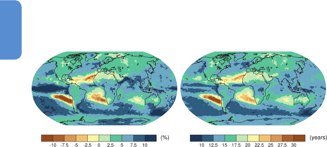
1086

Chapter 12 Long-term Climate Change: Projections, Commitments and Irreversibility

but there is strong agreement across the models over the direction of

change (Tebaldi et al., 2006; Goubanova and Li, 2007; Chen and Knut-

son, 2008; Haugen and Iversen, 2008; May, 2008b; Kysely and Berano-

va, 2009; Min et al., 2011; Sillmann et al., 2013). Regional details are

less robust in terms of the relative magnitude of changes but remain in

good accord across models in terms of the sign of the change and the

large-scale geographical patterns (Meehl et al., 2005a; CCSP, 2008a). In

semi-arid regions of the midlatitudes and subtropics such as the Medi-

terranean, the southwest USA, southwestern Australia, southern Africa

and a large portion of South America, the tendency manifested in the

majority of model simulations is for longer dry periods and is consist-

ent with the average decreases shown in Figure 12.22. Figure 12.26

shows projected percent changes in RX5day, the annual maximum of

consecutive 5-day precipitation over land regions obtained from the

CMIP5 models (Box 2.4, Table 1). Globally averaged end of 21st centu-

ry changes over land range from 5% (RCP2.6) to 20% (RCP8.5) more

precipitation during very wet 5-day periods. Results from the CMIP3

models are shown for comparison (see Section 12.4.9). Locally, the few

regions where this index of extreme precipitation decreases in the late

21st century RCP8.5 projection coincide with areas of robust decreases

in the mean precipitation of Figure 12.22.

Drought is discussed extensively in the SREX report (Seneviratne et al.,

2012) and the conclusions about future drought risk described there

based on CMIP3 models are reinforced by the CMIP5 models. As noted

in the SREX reports, assessments of changes in drought characteristics

with climate change should be made in the context of speciﬁc impacts

questions. The risk of future agricultural drought episodes is increased

in the regions of robust soil moisture decrease described in Section

12.4.5.3 and shown in Figure 12.23. Other measures in the literature of

future agricultural drought are largely focussed on the Palmer Drought

Severity Index (Wehner et al., 2011; Schwalm et al., 2012; Dai, 2013)

and project ‘extreme’ drought as the normal climatological state by

the end of the 21st century under the high emission scenarios in many

mid-latitude locations. However, this measure of agricultural drought

has been criticized as overly sensitive to increased temperatures due to

a simpliﬁed soil moisture model (Hoerling et al., 2012). The consecutive

dry-day index (CDD) is the length of the longest period of consecutive

days with precipitation less than 1 mm (Box 2.4, Table 1). CMIP5 pro-

jected changes in CDD over the 2081–2100 period under the RCP8.5

scenario (relative to the 1981–2000 reference period in common with

CMIP3) from the CMIP5 models are shown in Figure 12.26c and exhib-

it patterns similar to projected changes in both precipitation and soil

moisture (Sillmann et al., 2013). Substantial increases in this measure

of meteorological drought are projected in the Mediterranean, Central

America, Brazil, South Africa and Australia while decreases are project-

ed in high northern latitudes.

Truly rare precipitation events can cause very signiﬁcant impacts. The

statistics of these events at the tails of the precipitation distribution

are well described by Extreme Value (EV) Theory although there are sig-

niﬁcant biases in the direct comparison of gridded model output and

actual station data (Smith et al., 2009). There is also strong evidence

that model resolution plays a key role in replicating EV quantities esti-

mated from gridded observational data, suggesting that high-resolu-

tion models may provide somewhat more conﬁdence in projection of

changes in rare precipitation events (Fowler et al., 2007a; Wehner et

al., 2011). Figure 12.27 shows the late 21st century changes per degree

Celsius in local warming in 20-year return values of annual maximum

daily precipitation relative to the late 20th century (left) and the asso-

ciated return periods of late 20th century 20-year return values at the

end of the 21st century from the CMIP5 models. Across future emission

scenarios, the global average of the CMIP5 multi-model median return

value sensitivity is an increase of 5.3% °C

–1

(Kharin et al., 2013). The

CMIP5 land average is close to the CMIP3 value of 4% °C

–1

report-

ed by Min et al. (2011) for a subset of CMIP3 models. Corresponding

with this change, the global average of return periods of late 20th

century 20-year return values is reduced from 20 years to 14 years for

a 1°C local warming. Return periods are projected to be reduced by

about 10 to 20% °C

–1

over the most of the mid-latitude land masses

with larger reductions over wet tropical regions (Kharin et al., 2013).

Hence, extreme precipitation events will very likely be more intense

Daily precipitation 20-yr RV change per 1°C warming

RP for present day 20-yr RV of daily precipitation

under 1°C warming

31 31

Figure 12.27 | (Left) The CMIP5 2081–2100 multi-model ensemble median percent change in 20-year return values of annual maximum daily precipitation per 1°C of local warm-

ing relative to the 1986–2005 reference period. (Right) The average 2081–2100 CMIP5 multi-model ensemble median of the return periods (years) of 1986–2005 20-year return

values of annual maximum daily precipitation corresponding to 1°C of local warming. Regions of no change would have return periods of 20 years.

1087

Long-term Climate Change: Projections, Commitments and Irreversibility Chapter 12

and more frequent in these regions in a warmer climate. Reductions in

return values (or equivalently, increases in return period) are conﬁned

to convergent oceanic regions where circulation changes have reduced

the available water vapour.

Severe thunderstorms, associated with large hail, high winds, and tor-

nadoes, are another example of extreme weather associated with the

water cycle. The large-scale environments in which they occur are char-

acterized by large Convective Available Potential Energy (CAPE) and

deep tropospheric wind shear (Brooks et al., 2003; Brooks, 2009). Del

Genio et al. (2007), Trapp et al. (2007, 2009), and Van Klooster and Roe-

bber (2009) found a general increase in the energy and decrease in the

shear terms from the late 20th century to the late 21st century over the

USA using a variety of regional model simulations embedded in global

model SRES scenario simulations. The relative change between these

two competing factors would tend to favour more environments that

would support severe thunderstorms, providing storms are initiated.

Trapp et al. (2009), for example, found an increase in favourable thun-

derstorm conditions for all regions of the USA east of the Rocky Moun-

tains. Large variability in both the energy and shear terms means that

statistical signiﬁcance is not reached until late in the 21st century under

high forcing scenarios. One way of assessing the possibility of a change

in the frequency of future thunderstorms is to look at historical records

of observed tornado, hail and wind occurrence with respect to the envi-

ronmental conditions (Brooks, 2013). This indicates that an increase in

the fraction of severe thunderstorms containing non-tornadic winds

would be consistent with the model projections of increased energy

and decreased shear, but there has not been enough research to make

a ﬁrm conclusion regarding future changes in frequency or magnitude.

Less work has been done on projected changes outside of the USA.

Marsh et al. (2009) found that mean energy decreased in the warm

season in Europe while it increased in the cool season. Even though the

energy decreases in the warm season, the number of days with favour-

able environments for severe thunderstorms increases because of an

increasing number of days with relatively large values of available

energy. For Europe, with the Mediterranean Sea and Sahara Desert to

the south, questions remain about changes in boundary layer moisture,

a main driver of the energy term. Niall and Walsh (2005) examined

changes in CAPE, which may be associated with hailstorm occurrence

in southeastern Australia using a global model, and found little change

under warmer conditions. Leslie et al. (2008) reconsidered the south-

eastern Australia hail question by nesting models with 1 km horizontal

grid spacing and using sophisticated microphysical parameterizations

and found an increase in the frequency of large hail by 2050 under the

SRES A1B scenario, but with extremely large internal variability in the

environments and hail size.

Overall, for all parts of the world studied, the results are suggestive of

a trend toward environments favouring more severe thunderstorms,

but the small number of analyses precludes any likelihood estimate of

this change.

12.4.6 Changes in Cryosphere

12.4.6.1 Changes in Sea Ice Cover

Based on the analysis of CMIP3 climate change simulations (e.g., Arzel

et al., 2006; Zhang and Walsh, 2006), the AR4 concludes that the Arctic

and Antarctic sea ice covers are projected to shrink in the 21st cen-

tury under all SRES scenarios, with a large range of model responses

(Meehl et al., 2007b). It also stresses that, in some projections, the

Arctic Ocean becomes almost entirely ice-free in late summer during

the second half of the 21st century. These conclusions were conﬁrmed

by further analyses of the CMIP3 archives (e.g., Stroeve et al., 2007;

Bracegirdle et al., 2008; Lefebvre and Goosse, 2008; Boé et al., 2009b;

Sen Gupta et al., 2009; Wang and Overland, 2009; Zhang, 2010b; NRC,

2011; Körper et al., 2013). Figures 12.28 and 12.29 and the studies of

Maksym et al. (2012), Massonnet et al. (2012), Stroeve et al. (2012) and

Wang and Overland (2012) show that the CMIP5 AOGCMs/ESMs as a

group also project decreases in sea ice extent through the end of this

century in both hemispheres under all RCPs. However, as in the case of

CMIP3, the inter-model spread is considerable.

In the NH, in accordance with CMIP3 results, the absolute rate of

decrease of the CMIP5 multi-model mean sea ice areal coverage is

greatest in September. The reduction in sea ice extent between the

time periods 1986–2005 and 2081–2100 for the CMIP5 multi-model

average ranges from 8% for RCP2.6 to 34% for RCP8.5 in February

and from 43% for RCP2.6 to 94% for RCP8.5 in September. Medium

conﬁdence is attached to these values as projections of sea ice extent

decline in the real world due to errors in the simulation of present-day

sea ice extent (mean and trends—see Section 9.4.3) and because

of the large spread of model responses. About 90% of the available

CMIP5 models reach nearly ice-free conditions (sea ice extent less than

1 × 10

for at least 5 consecutive years) during September in the

Arctic before 2100 under RCP8.5 (about 45% under RCP4.5). By the

end of the 21st century, the decrease in multi-model mean sea ice

volume ranges from 29% for RCP2.6 to 73% for RCP8.5 in February

and from 54% for RCP2.6 to 96% for RCP8.5 in September. Medium

conﬁdence is attached to these values as projections of the real world

sea ice volume. In February, these percentages are much higher than

the corresponding ones for sea ice extent, which is indicative of a sub-

stantial sea ice thinning.

A frequent criticism of the CMIP3 models is that, as a group, they

strongly underestimate the rapid decline in summer Arctic sea ice

extent observed during the past few decades (e.g., Stroeve et al., 2007;

Winton, 2011), which suggests that the CMIP3 projections of summer

Arctic sea ice areal coverage might be too conservative. As shown in

Section 9.4.3 and Figure 12.28b, the magnitude of the CMIP5 mul-

ti-model mean trend in September Arctic sea ice extent over the satel-

lite era is more consistent with, but still underestimates, the observed

one (see also Massonnet et al., 2012; Stroeve et al., 2012; Wang and

Overland, 2012; Overland and Wang, 2013). Owing to the shortness of

the observational record, it is difﬁcult to ascertain the relative inﬂu-

ence of natural variability on this trend. This hinders the comparison

between modelled and observed trends, and hence the estimate of the

sensitivity of the September Arctic sea ice extent to global surface tem-

perature change (i.e., the decrease in sea ice extent per degree global

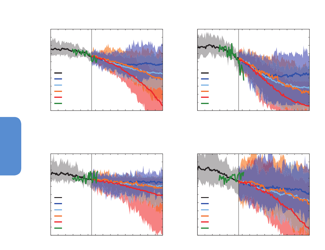
1088

Chapter 12 Long-term Climate Change: Projections, Commitments and Irreversibility

warming) (Kay et al., 2011; Winton, 2011; Mahlstein and Knutti, 2012).

This sensitivity may be crucial for determining future sea ice losses.

Indeed, a clear relationship exists at longer than decadal time scales

in climate change simulations between the annual mean or September

mean Arctic sea ice extent and the annual mean global surface tem-

perature change for ice extents larger than ~1 × 10

(e.g., Ridley

et al., 2007; Zhang, 2010b; NRC, 2011; Winton, 2011; Mahlstein and

Knutti, 2012). This relationship is illustrated in Figure 12.30 for both

CMIP3 and CMIP5 models. From this ﬁgure, it can be seen that the sea

ice sensitivity varies signiﬁcantly from model to model and is generally

larger and in better agreement among models in CMIP5.

A complete and detailed explanation for what controls the range of

Arctic sea ice responses in models over the 21st century remains elu-

sive, but the Arctic sea ice provides an example where process-based

constraints can be used to reduce the spread of model projections

Year

Sea ice extent change (10

)

Northern Hemisphere February

Satellite obs. 1986−2005 avg: 15.5 x 10

CMIP5 historical 1986−2005 avg: 15.9 x10

Historical (39)

Observations

RCP2.6 (29)

RCP4.5 (39)

RCP6.0 (21)

RCP8.5 (37)

1960 1980 2000 2020 2040 2060 2080 2100

−7

−6

−5

−4

−3

−2

−1

Year

Sea ice extent change (10

)

Northern Hemisphere September

Satellite obs. 1986−2005 avg: 7.1 x10

CMIP5 historical 1986−2005 avg: 6.6 x10

Historical (39)

Observations

RCP2.6 (29)

RCP4.5 (39)

RCP6.0 (21)

RCP8.5 (37)

1960 1980 2000 2020 2040 2060 2080 2100

−7

−6

−5

−4

−3

−2

−1

Year

Sea ice extent change (10

)

Southern Hemisphere February

Satellite obs. 1986−2005 avg: 3.3 x10

CMIP5 historical 1986−2005 avg: 3.0 x10

Historical (39)

Observations

RCP2.6 (29)

RCP4.5 (39)

RCP6.0 (21)

RCP8.5 (37)

1960 1980 2000 2020 2040 2060 2080 2100

−7

−6

−5

−4

−3

−2

−1

Year

Sea ice extent change (10

)

Southern Hemisphere September

Satellite obs. 1986−2005 avg: 19.0 x10

CMIP5 historical 1986−2005 avg: 17.8 x10

Historical (39)

Observations

RCP2.6 (29)

RCP4.5 (39)

RCP6.0 (21)

RCP8.5 (37)

1960 1980 2000 2020 2040 2060 2080 2100

−7

−6

−5

−4

−3

−2

−1

Figure 12.28 | Changes in sea ice extent as simulated by CMIP5 models over the second half of the 20th century and the whole 21st century under RCP2.6, RCP4.5, RCP6.0 and

RCP8.5 for (a) Northern Hemisphere February, (b) Northern Hemisphere September, (c) Southern Hemisphere February and (d) Southern Hemisphere September. The solid curves

show the multi-model means and the shading denotes the 5 to 95% range of the ensemble. The vertical line marks the end of CMIP5 historical climate change simulations. One

ensemble member per model is taken into account in the analysis. Sea ice extent is deﬁned as the total ocean area where sea ice concentration exceeds 15% and is calculated on

the original model grids. Changes are relative to the reference period 1986–2005. The number of models available for each RCP is given in the legend. Also plotted (solid green

curves) are the satellite data of Comiso and Nishio (2008, updated 2012) over 1979–2012.

(Overland et al., 2011; Collins et al., 2012; Hodson et al., 2012). For

CMIP3 models, results indicate that the changes in Arctic sea ice mass

budget over the 21st century are related to the late 20th century mean

sea ice thickness distribution (Holland et al., 2010), average sea ice

thickness (Bitz, 2008; Hodson et al., 2012), fraction of thin ice cover

(Boé et al., 2009b) and oceanic heat transport to the Arctic (Mahlstein

and Knutti, 2011). For CMIP5 models, Massonnet et al. (2012) showed

that the time needed for the September Arctic sea ice areal coverage to

drop below a certain threshold is highly correlated with the September

sea ice extent and annual mean sea ice volume averaged over the past

several decades (Figure 12.31a, b). The timing of a seasonally ice-free

Arctic Ocean or the fraction of remaining sea ice in September at any

time during the 21st century were also found to correlate with the

past trend in September Arctic sea ice extent and the amplitude of the

mean seasonal cycle of sea ice extent (Boé et al., 2009b; Collins et al.,

2012; Massonnet et al., 2012) (Figure 12.31c, d). All these empirical

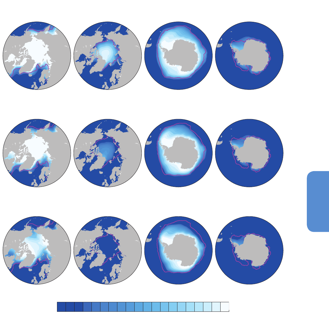
1089

Long-term Climate Change: Projections, Commitments and Irreversibility Chapter 12

Figure 12.29 | February and September CMIP5 multi-model mean sea ice concentrations (%) in the Northern and Southern Hemispheres for the periods (a) 1986–2005, (b)

taken into account in the analysis, and the multi-model mean sea ice concentration is shown where it is larger than 15%. The number of models available for each RCP is given in

parentheses. The pink lines indicate the observed 15% sea ice concentration limits averaged over 1986–2005 (Comiso and Nishio, 2008, updated 2012).

relationships can be understood on simple physical grounds (see the

aforementioned references for details).

These results lend support for weighting/recalibrating the models

based on their present-day Arctic sea ice simulations. Today, the opti-

mal approach for constraining sea ice projections from climate models

is unclear, although one notes that these methods should have a

credible underlying physical basis in order to increase conﬁdence in

their results (see Section 12.2). In addition, they should account for

February September September February

a) 1986−2005 average (39)

b) 2081−2100 average, RCP4.5 (39)

c) 2081−2100 average, RCP8.5 (37)

(%)

0 20 40 60 80 100

the potentially large imprint of natural variability on both observations

and model simulations when these two sources of information are to

be compared (see Section 9.8.3). This latter point is particularly critical

if the past sea ice trend or sensitivity is used in performance metrics

given the relatively short observational period (Kay et al., 2011; Over-

land et al., 2011; Mahlstein and Knutti, 2012; Massonnet et al., 2012;

Stroeve et al., 2012). A number of studies have applied such metrics

to the CMIP3 and CMIP5 models. Stroeve et al. (2007) and Stroeve et

al. (2012) rejected several CMIP3 and CMIP5 models, respectively, on

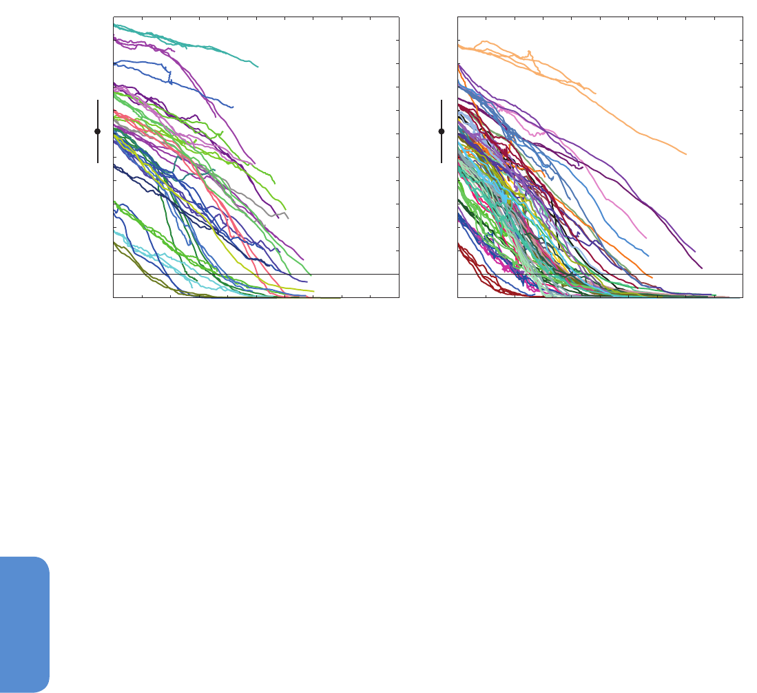
1090

Chapter 12 Long-term Climate Change: Projections, Commitments and Irreversibility

the basis of their simulated late 20th century mean September Arctic

sea ice extent. Wang and Overland (2009) selected a subset of CMIP3

models (and Wang and Overland (2012) did the same for the CMIP5

models) based on their ﬁdelity to the observed mean seasonal cycle of

Arctic sea ice extent in the late 20th century and then scaled the chosen

models to the recently observed September sea ice extent. Zhang

(2010b) retained a number of CMIP3 models based on the regression

between summer sea ice loss and Arctic surface temperature change.

Boé et al. (2009b) and Mahlstein and Knutti (2012) did not perform a

model selection but rather recalibrated the CMIP3 Arctic sea ice projec-

tions on available observations of September Arctic sea ice trend and

sensitivity to global surface temperature change, respectively. Finally,

Massonnet et al. (2012) selected a subset of CMIP5 models on the

basis of the four relationships illustrated in Figure 12.31a–d.

These various methods all suggest a faster rate of summer Arctic sea

ice decline than the multi-model mean. Although they individually

provide a reduced range for the year of near disappearance of the

September Arctic sea ice compared to the original CMIP3/CMIP5 mul-

ti-model ensemble, they lead to different timings (Overland and Wang,

2013). Consequently, the time interval obtained when combining all

these studies remains wide: 2020–2100

(2100

= not before 2100)

for the SRES A1B scenario and RCP4.5 (Stroeve et al., 2007, 2012; Boé

et al., 2009b; Wang and Overland, 2009, 2012; Zhang, 2010b; Masson-

net et al., 2012) and 2020–2060 for RCP8.5 (Massonnet et al., 2012;

Wang and Overland, 2012). The method proposed by Massonnet et

al. (2012) is applied here to the full set of models that provided the

CMIP5 database with sea ice output. The natural variability of each

of the four diagnostics shown in Figure 12.31a–d is ﬁrst estimated

by averaging over all available models with more than one ensemble

member the diagnostic standard deviations derived from the model

CMIP5 (b)

Annual mean global surface warming (°C)

September Arctic sea ice extent (10

)

0 1 2 3 4 5

CMIP3 (a)

Annual mean global surface warming (°C)

September Arctic sea ice extent (10

)

0 1 2 3 4 5

Figure 12.30 | September Arctic sea ice extent as a function of the annual mean global surface warming relative to the period 1986–2005 for (a) CMIP3 models (all SRES sce-

narios) and (b) CMIP5 models (all RCPs). The ice extents and global temperatures are computed on a common latitude-longitude grid for CMIP3 and on the original model grids for

CMIP5. One ensemble member per model is taken into account in the analysis. A 21-year running mean is applied to the model output. The full black circle and vertical bar on the

left-hand side of the y-axis indicate the mean and ±2 standard deviations about the mean of the observed September Arctic sea ice extent over 1986–2005, respectively (Comiso

and Nishio, 2008, updated 2012). The horizontal line corresponds to a nearly ice-free Arctic Ocean in September.

ensemble members. Then, for each model, a ±2 standard deviation

interval is constructed around the ensemble mean or single realization

of the diagnostic considered. A model is retained if, for each diagnostic,

either this interval overlaps a ±20% interval around the observed/rea-

nalysed value of the diagnostic or at least one ensemble member from

that model gives a value for the diagnostic that falls within ±20% of

the observational/reanalysed data. The outcome is displayed in Figure

12.31e for RCP8.5. Among the ﬁve selected models (ACCESS1.0,

ACCESS1.3, GFDL-CM3, IPSL-CM5A-MR, MPI-ESM-MR), four project

a nearly ice-free Arctic Ocean in September before 2050 (2080) for

RCP8.5 (RCP4.5), the earliest and latest years of near disappearance

of the sea ice pack being about 2040 and about 2060 (about 2040

and 2100

), respectively. It should be mentioned that Maslowski et al.

(2012) projected that it would take only until about 2016 to reach a

nearly ice-free Arctic Ocean in summer, based on a linear extrapolation

into the future of the recent sea ice volume trend from a hindcast sim-

ulation conducted with a regional model of the Arctic sea ice–ocean

system. However, such an extrapolation approach is problematic as it

ignores the negative feedbacks that can occur when the sea ice cover

becomes thin (e.g., Bitz and Roe, 2004; Notz, 2009) and neglects the

effect of year-to-year or longer-term variability (Overland and Wang,

2013). Mahlstein and Knutti (2012) encompassed the dependence of

sea ice projections on the forcing scenario by determining the annual

mean global surface warming threshold for nearly ice-free conditions

in September. Their best estimate of ~2°C above the present derived

from both CMIP3 models and observations is consistent with the 1.6

to 2.1°C range (mean value: 1.9°C) obtained from the CMIP5 model

subset shown in Figure 12.31e (see also Figure 12.30b). The reduction

in September Arctic sea ice extent by the end of the 21st century, aver-

aged over this subset of models, ranges from 56% for RCP2.6 to 100%

for RCP8.5.

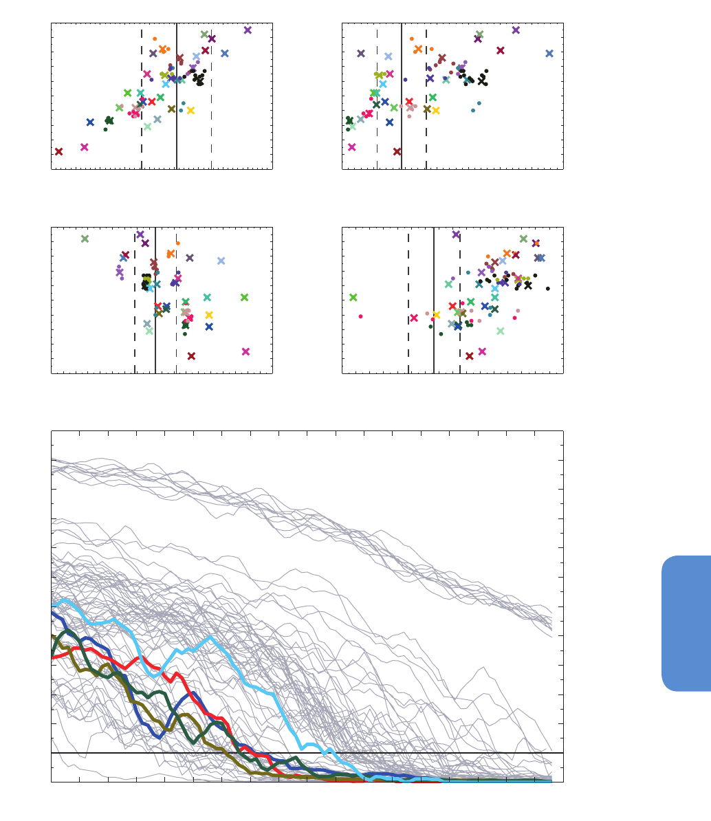
1091

Long-term Climate Change: Projections, Commitments and Irreversibility Chapter 12

Figure 12.31 | (a–d) First year during which the September Arctic sea ice extent falls below 1 × 10

in CMIP5 climate projections (37 models, RCP8.5) as a function of (a)

the September Arctic sea ice extent averaged over 1986–2005, (b) the annual mean Arctic sea ice volume averaged over 1986–2005, (c) the amplitude of the 1986–2005 mean

seasonal cycle of Arctic sea ice extent and (d) the trend in September Arctic sea ice extent over 1979–2012. The sea ice diagnostics displayed are calculated on the original model

grids. The correlations and one-tailed p-values are computed from the multi-member means for models with several ensemble members (coloured crosses), but the ensemble mem-

bers of individual models are also depicted (coloured dots). The vertical solid and dashed lines show the corresponding observations or bias-adjusted PIOMAS (Pan-Arctic Ice-Ocean

Modelling and Assimilation System) reanalysis data (a, c and d: Comiso and Nishio, 2008, updated 2012; b: Schweiger et al., 2011) and the ±20% interval around these data,

respectively. (e) Time series of September Arctic sea ice extent (5-year running mean) as simulated by all CMIP5 models and their ensemble members under RCP8.5 (thin curves).

The thick, coloured curves correspond to a subset of ﬁve CMIP5 models selected on the basis of panels a–d following Massonnet et al. (2012) (see text for details). Note that each

of these models provides only one ensemble member for RCP8.5.

RCP8.5, correlation = 0.82, p = 1e−09

September Arctic sea ice extent

averaged over 1986−2005 (10

)

2 3 4 5 6 7 8 9 10 11

2000

2020

2040

2060

2080

2100

RCP8.5, correlation = 0.64, p = 2e−05

Annual mean Arctic sea ice volume

averaged over 1986−2005 (10

)

10 15 20 25 30 35 40 45

2000

2020

2040

2060

2080

2100

RCP8.5, correlation = −0.53, p = 0.0007

Amplitude of the seasonal cycle of Arctic sea ice extent

averaged over 1986−2005 (10

)

First year of near disappearance of September Arctic sea ice

0 2 4 6 8 10 12 14 16 18

2000

2020

2040

2060

2080

2100

RCP8.5, correlation = 0.48, p = 0.002

Trend in September Arctic sea ice extent

over 1979−2012 (10

/decade)

−1600 −1200 −800 −400 0

2000

2020

2040

2060

2080

2100

Year

September Arctic sea ice extent (10

)

RCP8.5

2010 2020 2030 2040 2050 2060 2070 2080 2090 2100

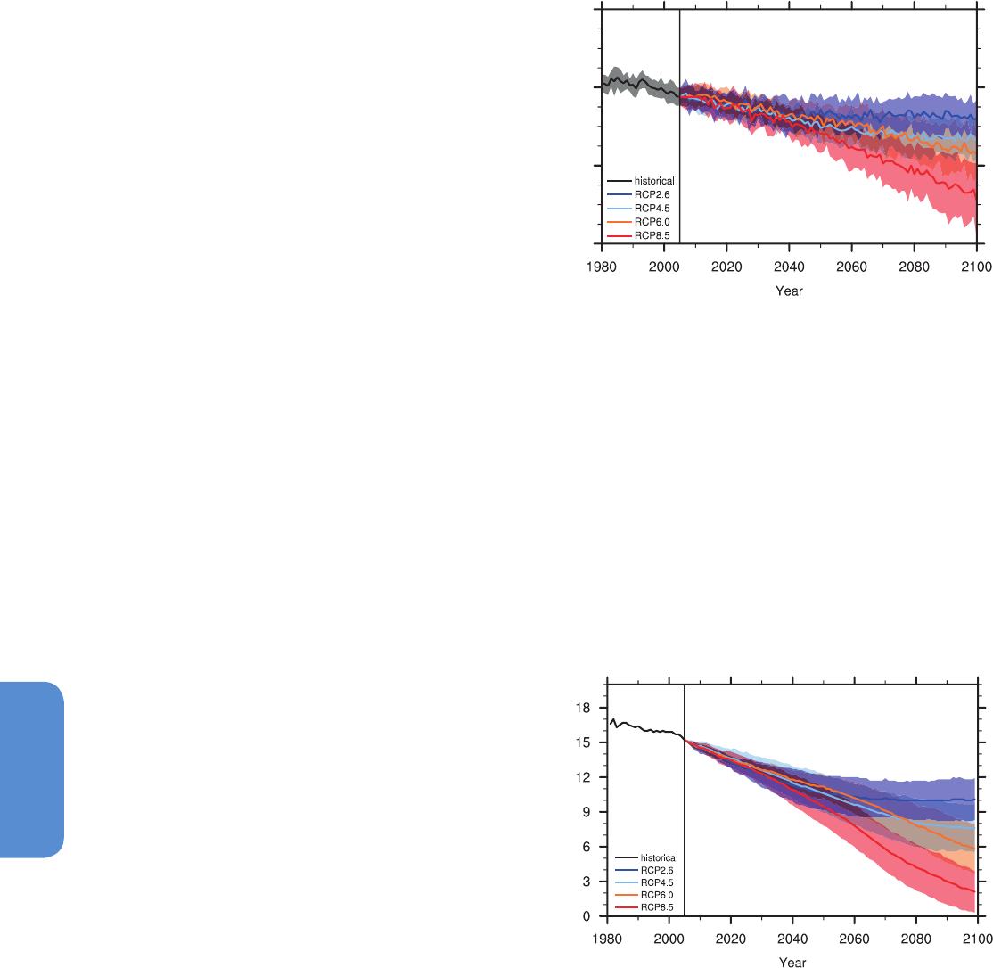
1092

Chapter 12 Long-term Climate Change: Projections, Commitments and Irreversibility

In light of all these results, it is very likely that the Arctic sea ice cover

will continue to shrink and thin all year round during the 21st century

as the annual mean global surface temperature rises. It is also likely

that the Arctic Ocean will become nearly ice-free in September before

the middle of the century for high GHG emissions such as those corre-

sponding to RCP8.5 (medium conﬁdence). The potential irreversibility

of the Arctic sea ice loss and the possibility of an abrupt transition

toward an ice-free Arctic Ocean are discussed in Section 12.5.5.7.

In the SH, the decrease in sea ice extent between 1986–2005 and

2081–2100 projected by the CMIP5 models as a group varies from

16% for RCP2.6 to 67% for RCP8.5 in February and from 8% to 30%

in September. In contrast with the NH, the absolute rate of decline is

greatest in wintertime. Eisenman et al. (2011) argue that this hemi-

spheric asymmetry in the seasonality of sea ice loss is fundamentally

related to the geometry of coastlines. For each forcing scenario, the

relative changes in multi-model mean February and September Antarc-

tic sea ice volumes by the end of the century are of the same order as

the corresponding ones for sea ice extent. About 75% of the available

CMIP5 models reach a nearly ice-free state in February within this cen-

tury under RCP8.5 (about 60% under RCP4.5). For RCP8.5, only small

portions of the Weddell and Ross Seas stay ice-covered in February

during 2081–2100 in those models that do not project a seasonally

ice-free Southern Ocean (see Figure 12.29c). Nonetheless, there is low

conﬁdence in these Antarctic sea ice projections because of the wide

range of model responses and the inability of almost all of the models

to reproduce the mean seasonal cycle, interannual variability and over-

all increase of the Antarctic sea ice areal coverage observed during the

satellite era (see Section 9.4.3; Maksym et al., 2012; Turner et al., 2013;

Zunz et al., 2013).

12.4.6.2 Changes in Snow Cover and Frozen Ground

Excluding ice sheets and glaciers, analyses of seasonal snow cover

changes generally focus on the NH, where the conﬁguration of the

continents on the Earth induces a larger maximum seasonal snow

cover extent (SCE) and a larger sensitivity of SCE to climate changes.

Seasonal snow cover extent and snow water equivalent (SWE) respond

to both temperature and precipitation. At the beginning and the end

of the snow season, SCE decreases are closely linked to a shortening

of the seasonal snow cover duration, while SWE is more sensitive to

snowfall amount (Brown and Mote, 2009). Future widespread reduc-

tions of SCE, particularly in spring, are simulated by the CMIP3 models

(Roesch, 2006; Brown and Mote, 2009) and conﬁrmed by the CMIP5

ensemble (Brutel-Vuilmet et al., 2013). The NH spring (March-April

average) snow cover area changes are coherent in the CMIP5 models

although there is considerable scatter. Relative to the 1986–2005 ref-

erence period, the CMIP5 models simulate a weak decrease of about

7 ± 4% (one-σ inter-model dispersion) for RCP2.6 during the last two

decades of the 21st century, while SCE decreases of about 13 ± 4% are

simulated for RCP4.5, 15 ± 5% for RCP6.0, and 25 ± 8% for RCP8.5

(Figure 12.32). There is medium conﬁdence in these numbers because

of the considerable inter-model scatter mentioned above and because

snow processes in global climate models are strongly simpliﬁed.

Projections for the change in annual maximum SWE are more mixed.

Warming decreases SWE both by reducing the fraction of precipitation

that falls as snow and by increasing snowmelt, but projected increas-

es in precipitation over much of the northern high latitudes during

winter months act to increase snow amounts. Whether snow cover-

ing the ground will become thicker or thinner depends on the balance

between these competing factors. Both in the CMIP3 (Räisänen, 2008)

and in the CMIP5 models (Brutel-Vuilmet et al., 2013), annual maxi-

mum SWE tends to increase or only marginally decrease in the coldest

-20

-40

(%)

Snow cover extent change

Figure 12.32 | Northern Hemisphere spring (March to April average) snow cover

extent change (in %) in the CMIP5 ensemble, relative to the simulated extent for the

1986–2005 reference period. Thick lines mark the multi-model average, shading indi-

cates the inter-model spread (one standard deviation). The observed March to April

average snow cover extent for the 1986–2005 reference period is 32.6·10

(Brown

and Robinson, 2011).

Near-surface permafrost area

(10

)

Figure 12.33 | Northern Hemisphere near-surface permafrost area, diagnosed for

the available CMIP5 models by Slater and Lawrence (2013) following Nelson and Out-

calt (1987) and using 20-year average bias-corrected monthly surface air temperatures

and snow depths. Thick lines: multi-model average. Shading and thin lines indicate the

inter-model spread (one standard deviation). The black line for the historical period is

diagnosed from the average of the European Centre for Medium range Weather Fore-

cast (ECMWF) reanalysis of the global atmosphere and surface conditions (ERA), Japa-

nese ReAnalysis (JRA), Modern Era Retrospective-analysis for Research and Applications

(MERRA) and Climate Forecast System Reanalysis and Reforecast (CFSRR) reanalyses

(Slater and Lawrence, 2013). Estimated present permafrost extent is between 12 and

17 million km

(Zhang et al., 2000).

1093

Long-term Climate Change: Projections, Commitments and Irreversibility Chapter 12

regions, while annual maximum SWE decreases are strong closer to the

southern limit of the seasonally snow-covered area.

It is thus very likely (high conﬁdence) that by the end of the 21st centu-

ry, NH spring snow cover extent will be substantially lower than today

if anthropogenic climate forcing is similar to the stronger scenarios

considered here. Conversely, there is only medium conﬁdence in the

latitudinal pattern of annual maximum SWE changes (increase or little

change in the coldest regions, stronger decrease further to the South)

because annual maximum SWE is inﬂuenced by competing factors

(earlier melt onset, higher solid precipitation rates in some regions).

The strong projected warming across the northern high latitudes in

climate model simulations has implications for frozen ground. Recent

projections of the extent of near-surface permafrost (see Glossary)

degradation continue to vary widely depending on the underlying

climate forcing scenario and model physics, but virtually all of them

indicate substantial near-surface permafrost degradation and thaw

depth deepening over much of the permafrost area (Saito et al., 2007;

Lawrence et al., 2008a, 2012; Koven et al., 2011, 2013; Eliseev et al.,

2013; Slater and Lawrence, 2013). Permafrost at greater depths is less

directly relevant to the surface energy and water balance, and its deg-

radation naturally occurs much more slowly (Delisle, 2007). Climate

models are beginning to represent permafrost physical processes and

properties more accurately (Alexeev et al., 2007; Nicolsky et al., 2007;

Lawrence et al., 2008a; Rinke et al., 2008; Koven et al., 2009; Gout-

tevin et al., 2012), but there are large disagreements in the calculation

of current frozen soil extent and active layer depth due to differenc-

es in the land model physics in the CMIP5 ensemble (Koven et al.,

2013). The projected changes in permafrost are a response not only

to warming, but also to changes in snow conditions because snow

properties and their seasonal evolution exert signiﬁcant control on soil

thermal state (Zhang, 2005; Lawrence and Slater, 2010; Shkolnik et

al., 2010; Koven et al., 2013). Applying the surface frost index method

(Nelson and Outcalt, 1987) to coupled climate model anomalies from

the CMIP5 models (Slater and Lawrence, 2013) yields a reduction of

the diagnosed 2080–2099 near-surface permafrost area (continuous

plus discontinuous near-surface permafrost) by 37 ± 11% (RCP2.6),

51 ± 13% (RCP4.5), 58 ± 13% (RCP6.0), and 81±12% (RCP8.5), com-

pared to the 1986–2005 diagnosed near-surface permafrost area, with

medium conﬁdence in the numbers as such because of the strongly

simpliﬁed soil physical processes in current-generation global climate

models (Figure 12.33). The uncertainty range given here is the 1-σ

inter-model dispersion. Applying directly the model output to diag-

nose permafrost extent and its changes over the 21st century yields

similar relative changes (Koven et al., 2013). In summary, based on

high agreement across CMIP5 and older model projections, fundamen-

tal process understanding, and paleoclimatic evidence (e.g., Vaks et

al., 2013), it appears virtually certain (high conﬁdence) that near-sur-

face permafrost extent will shrink as global climate warms. However,

the amplitude of the projected reductions of near-surface permafrost

extent not only depends on the emission scenario and the global cli-

mate model response, but also very much on the permafrost-related

soil processes taken into account in the models.

12.4.7 Changes in the Ocean

12.4.7.1 Sea Surface Temperature, Salinity and Ocean

Heat Content

Projected increase of SST and heat content over the next two decades

is relatively insensitive to the emissions trajectory. However, projected

outcomes diverge as the 21st century progresses. When SSTs increase

as a result of external forcing, the interior water masses respond to

the integrated signal at the surface, which is then propagated down to

greater depth (Gleckler et al., 2006; Gregory, 2010). Changes in glob-

ally averaged ocean heat content currently account for about 90% of

the change in global energy inventory since 1970 (see Box 3.1). Heat is

transported within the interior of the ocean by its large-scale general

circulation and by smaller-scale mixing processes. Changes in trans-

ports lead to redistribution of existing heat content and can cause local

cooling even though the global mean heat content is rising (Banks and

Gregory, 2006; Lowe and Gregory, 2006; Xie and Vallis, 2012).

Figure 12.12 shows the multi-model mean projections of zonally aver-

aged ocean temperature change under three emission scenarios. The

differences in projected ocean temperature changes for different RCPs

manifest themselves more markedly as the century progresses. The

largest warming is found in the top few hundred metres of the subtrop-

ical gyres, similar to the observed pattern of ocean temperature chang-

es (Levitus et al., 2012, see also Section 3.2). Surface warming varies

considerably between the emission scenarios ranging from about 1°C

(RCP2.6) to more than 3°C in RCP8.5. Mixing and advection processes

gradually transfer the additional heat to deeper levels of about 2000

m at the end of the 21st century. Depending on the emission scenario,

global ocean warming between 0.5°C (RCP2.6) and 1.5°C (RCP8.5)

will reach a depth of about 1 km by the end of the century. The stron-

gest warming signal is found at the surface in subtropical and tropical

regions. At depth the warming is most pronounced in the Southern

Ocean. From an energy point of view, for RCP4.5 by the end of the 21st

century, half of the energy taken up by the ocean is in the uppermost

700 m, and 85% is in the uppermost 2000 m.

In addition to the upper-level warming, the patterns are further char-

acterized by a slight cooling in parts of the northern mid- and high

latitudes below 1000 m and a pronounced heat uptake in the deep

Southern Ocean at the end of the 21st century. The cooling may be

linked to the projected decrease of the strength of the AMOC (see Sec-

tion 12.4.7.2; 13.4.1; Banks and Gregory, 2006).

The response of ocean temperatures to external forcing comprises

mainly two time scales: a relatively fast adjustment of the ocean mixed

layer and the slow response of the deep ocean (Hansen et al., 1985;

Knutti et al., 2008a; Held et al., 2010). Simulations with coupled ocean–

atmosphere GCMs suggest time-scales of several millennia until the

deep ocean is in equilibrium with the external forcing (Stouffer, 2004;

Hansen et al., 2011; Li et al., 2013a). Thus, the long time-scale of the

ocean response to external forcing implies an additional commitment

to warming for many centuries when GHG emissions are decreased or

concentrations kept constant (see Section 12.5.2). Further assessment

of ocean heat uptake and its relationship to projections of sea level rise

is presented in Section 13.4.1.

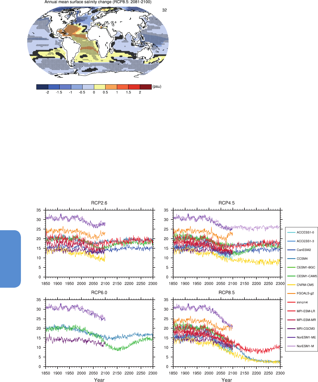
1094

Chapter 12 Long-term Climate Change: Projections, Commitments and Irreversibility

Durack and Wijffels (2010) and Durack et al. (2012) examined trends

in global sea surface salinity (SSS) changes over the period 1950–

2008. Their analysis revealed strong, spatially coherent trends in SSS

over much of the global ocean, with a pattern that bears striking

resemblance to the climatological SSS ﬁeld and is associated with an

intensiﬁcation of the global water cycle (see Sections 3.3.2.1, 10.4.2

and 12.4.5). The CMIP5 climate model projections available suggest

that high SSS subtropical regions that are dominated by net evapora-

tion are typically getting more saline; lower SSS regions at high lati-

tudes are typically getting fresher. They also suggest a continuation

of this trend in the Atlantic where subtropical surface waters become

more saline as the century progresses (Figure 12.34) (see also Terray et

al., 2012). At the same time, the North Paciﬁc is projected to become

less saline.

12.4.7.2 Atlantic Meridional Overturning

Almost all climate model projections reveal an increase of high latitude

temperature and high latitude precipitation (Meehl et al., 2007b). Both

of these effects tend to make the high latitude surface waters lighter

and hence increase their stability. As seen in Figure 12.35, all models

show a weakening of the AMOC over the course of the 21st century

(see Section 12.5.5.2 for further analysis). Projected changes in the

strength of the AMOC at high latitudes appear stronger in Geophysical

Fluid Dynamics Laboratory (GFDL) CM2.1 when density is used as a

vertical coordinate instead of depth (Zhang, 2010a). Once the RF is sta-

bilized, the AMOC recovers, but in some models to less than its pre-in-

dustrial level. The recovery may include a signiﬁcant overshoot (i.e., a

weaker circulation may persist) if the anthropogenic RF is eliminated

(Wu et al., 2011a). Gregory et al. (2005) found that for all eleven models

Figure 12.34 | Projected sea surface salinity differences 2081–2100 for RCP8.5 rela-

tive to 1986–2005 from CMIP5 models. Hatching indicates regions where the multi-

model mean change is less than one standard deviation of internal variability. Stippling

indicates regions where the multi-model mean change is greater than two standard

deviations of internal variability and where at least 90% of the models agree on the

sign of change (see Box 12.1). The number of CMIP5 models used is indicated in the

upper right corner.

Atlantic Meridional Overturning Circulation at 30

(Sv)(Sv)

Figure 12.35 | Multi-model projections of Atlantic Meridional Overturning Circulation (AMOC) strength at 30°N from 1850 through to the end of the RCP extensions. Results are

based on a small number of CMIP5 models available. Curves show results from only the ﬁrst member of the submitted ensemble of experiments.

1095

Long-term Climate Change: Projections, Commitments and Irreversibility Chapter 12

analysed (six from CMIP2/3 and ﬁve EMICs), the AMOC reduction was

caused more by changes in surface heat ﬂux than changes in surface

freshwater ﬂux. They further found that models with a stronger AMOC

in their control run exhibited a larger weakening (see also Gregory and

Tailleux, 2011).

Based on the assessment of the CMIP5 RCP simulations and on our

understanding gleaned from analysis of CMIP3 models, observations

and our understanding of physical mechanisms, it is very likely that the

AMOC will weaken over the 21st century. Best estimates and ranges

for the reduction from CMIP5 are 11% (1 to 24%) in RCP2.6 and 34%

(12 to 54%) in RCP8.5. There is low conﬁdence in assessing the evolu-

tion of the AMOC beyond the 21st century.

12.4.7.3 Southern Ocean

A dominant and robust feature of the CMIP3 climate projections

assessed in AR4 is the weaker surface warming at the end of the 21st

century in the Southern Ocean area compared to the global mean. Fur-

thermore, the Antarctic Circumpolar Current (ACC) moves southward

in most of the climate projections analysed in response to the simulat-

ed southward shift and strengthening of the SH mid-latitude westerlies

(Meehl et al., 2007b).

The additional analyses of the CMIP3 model output performed since

the release of AR4 conﬁrm and reﬁne the earlier ﬁndings. The displace-

ment and intensiﬁcation of the mid-latitude westerlies contribute to a

large warming between 40°S and 60°S from the surface to mid-depths

(Fyfe et al., 2007; Sen Gupta et al., 2009). Part of this warming has

been attributed to the southward translation of the Southern Ocean

current system (Sen Gupta et al., 2009). Moreover, the wind changes

inﬂuence the surface temperature through modiﬁcations of the latent

and sensible heat ﬂuxes and force a larger northward Ekman trans-

port of relatively cold polar surface water (Screen et al., 2010). This

also leads to a stronger upwelling that brings southward and upward

relatively warm and salty deep water, resulting in a subsurface salinity

increase at mid-depths south of 50°S (Sen Gupta et al., 2009; Screen

et al., 2010).

Overall, CMIP3 climate projections exhibit a decrease in mixed layer

depth at southern mid- and high latitudes by the end of the 21st centu-

ry. This feature is a consequence of the enhanced stratiﬁcation resulting

from surface warming and freshening (Lefebvre and Goosse, 2008; Sen

Gupta et al., 2009; Capotondi et al., 2012). Despite large inter-mod-

el differences, there is a robust weakening of Antarctic Bottom Water

production and its northward outﬂow, which is consistent with the

decrease in surface density and is manifest as a warming signal close

to the Antarctic margin that reaches abyssal depths (Sen Gupta et al.,

2009).

In the vicinity of the Antarctic ice sheet, CMIP3 models project an aver-

age warming of ~0.5C° at depths of 200–500 m in 2091–2100 com-

pared to 1991–2000 for the SRES A1B scenario, which has the poten-

tial to impact the mass balance of ice shelves (Yin et al., 2011). More

detailed regional modelling using the SRES A1B scenario indicates

that a redirection of the coastal current into the cavities underlying

the Filchner-Ronne ice shelf during the second half of the 21st century

might enhance the average basal melting rate there from 0.2 m yr

–1

almost 4 m yr

–1

(Hellmer et al., 2012; see Section 13.4.4.2).

There are very few published analyses of CMIP5 climate projections

focusing on the Southern Ocean. Meijers et al. (2012) found a wide

variety of ACC responses to climate warming scenarios across CMIP5

models. Models show a high correlation between the changes in

ACC strength and position, with a southward (northward) shift of the

ACC core as the ACC gets stronger (weaker). No clear relationship

between future changes in wind stress and ACC strength was identi-

ﬁed, while the weakening of the ACC transport simulated at the end

of the 21st century by many models was found to correlate with the

strong decrease in the surface heat and freshwater ﬂuxes in the ACC

region (Meijers et al., 2012; Downes and Hogg, 2013). In agreement

with the CMIP3 assessment (Sen Gupta et al., 2009), subtropical gyres

generally strengthen under RCP4.5 and RCP8.5 and all expand south-

ward, inducing a southward shift of the northern boundary of the ACC

at most longitudes in the majority of CMIP5 models (Meijers et al.,

2012). As in CMIP3 climate projections, an overall shallowing of the

deep mixed layers that develop on the northern edge of the ACC in

winter is observed, with larger shallowing simulated by models with

deeper mixed layers during 1976–2005 (Sallée et al., 2013a). Sallée

et al. (2013b) reported a warming of all mode, intermediate and deep

water masses in the Southern Ocean. The largest temperature increase

is found in mode and intermediate water layers. Consistently with

CMIP3 projections (Downes et al., 2010), these water layers experience

a freshening, whereas bottom water becomes slightly saltier. Finally,

Sallée et al. (2013b) noted an enhanced upwelling of circumpolar deep

water and an increased subduction of intermediate water that are

nearly balanced by interior processes (diapycnal ﬂuxes).

A number of studies suggest that oceanic mesoscale eddies might

inﬂuence the response of the Southern Ocean circulation, meridional

heat transport and deep water formation to changes in wind stress and

surface buoyancy ﬂux (Böning et al., 2008; Farneti et al., 2010; Downes

et al., 2011; Farneti and Gent, 2011; Saenko et al., 2012; Spence et al.,

2012). These eddies are not explicitly resolved in climate models and

their role in future circulation changes still needs to be precisely quan-

tiﬁed. Some of the CMIP5 models have output the meridional overturn-

ing due to the Eulerian mean circulation and that induced by parame-

terized eddies, thus providing a quantitative estimate of the role of the

mesoscale circulation in a warming climate. On this basis, Downes and

Hogg (2013) found that, under RCP8.5, the strengthening (weakening)

of the upper (lower) Eulerian mean meridional overturning cell in the

Southern Ocean is signiﬁcantly correlated with the increased overlying

wind stress and surface warming and is partly compensated at best by

changes in eddy-induced overturning.

None of the CMIP3 and CMIP5 models include an interactive ice sheet

component. When climate-ice sheet interactions are accounted for in

an EMIC under a 4 × CO

scenario, the meltwater ﬂux from the Antarc-

tic ice sheet further reduces the surface density close to Antarctica and

the rate of Antarctic Bottom Water formation. This ultimately results

in a smaller surface warming at high southern latitudes compared to

a simulation in which the freshwater ﬂux from the melting ice sheet is

not taken into account (Swingedouw et al., 2008). Nevertheless, in this

study, this effect becomes signiﬁcant only after more than one century.

1096

Chapter 12 Long-term Climate Change: Projections, Commitments and Irreversibility

12.4.8 Changes Associated with Carbon Cycle Feedbacks

and Vegetation Cover

Climate change may affect the global biogeochemical cycles changing

the magnitude of the natural sources and sinks of major GHGs. Numer-

ous studies investigated the interactions between climate change and

the carbon cycle (e.g., Friedlingstein et al., 2006), methane cycle (e.g.,

O’Connor et al., 2010), ozone (Cionni et al., 2011) or aerosols (e.g.,

Carslaw et al., 2010). Many CMIP5 ESMs now include a representa-

tion of the carbon cycle as well as atmospheric chemistry, allowing

interactive projections of GHGs (mainly CO

and O

) and aerosols. With

such models, projections account for the imposed changes in anthro-

pogenic emissions, but also for changes in natural sources and sinks

as they respond to changes in climate and atmospheric composition. If

included in ESMs, the impact on projected concentration, RF and hence

on climate can be quantiﬁed. Climate-induced changes on the carbon

cycle are assessed below, while changes in natural emissions of CH

are assessed in Chapter 6, changes in atmospheric chemistry in Chap-

ter 11, and climate–aerosol interactions are assessed in Chapter 7.

12.4.8.1 Carbon Dioxide

As presented in Section 12.3, the CMIP5 experimental design includes,

for the RCP8.5 scenario, experiments driven either by prescribed

anthropogenic CO

emissions or concentration. The historical and

21st century emission-driven simulations allow evaluating the cli-

mate response of the Earth system when atmospheric CO

and the cli-

mate response are interactively being calculated by the ESMs. In such

ESMs, the atmospheric CO

is calculated as the difference between

the imposed anthropogenic emissions and the sum of land and ocean

carbon uptakes. As most of these ESMs account for land use changes

and their CO

emissions, the only external forcing is fossil fuel CO

emissions (along with all non-CO

forcings as in the C-driven RCP8.5

simulations). For a given ESM, the emission driven and concentration

driven simulations would show different climate projections if the

simulated atmospheric CO

in the emission driven run is signiﬁcantly

different from the one prescribed for the concentration driven runs.

This would happen if the ESMs carbon cycle is different from the one

simulated by MAGICC6, the model used to calculate the CMIP5 GHGs

concentrations from the emissions for the four RCPs (Meinshausen et

al., 2011c). When driven by CO

concentration, the ESMs can calculate

the fossil fuel CO

emissions that would be compatible with the pre-

scribed atmospheric CO

trajectory, allowing comparison with the set

of CO

emissions initially estimated by the IAMs (Arora et al., 2011;

Jones et al., 2013) (see Section 6.4.3, Box 6.4).

Figure 12.36 shows the simulated atmospheric CO

and global aver-

age surface air temperature warming (relative to the 1986–2005 ref-

erence period) for the RCP8.5 emission driven simulations from the

CMIP5 ESMs, compared to the concentration driven simulations from

the same models. Most (seven out of eleven) of the models estimate a

larger CO

concentration than the prescribed one. By 2100, the multi-

model average CO

concentration is 985 ± 97 ppm (full range 794

to 1142 ppm), while the CO

concentration prescribed for the RCP8.5

is 936 ppm. Figure 12.36 also shows the range of atmospheric CO

projections when the MAGICC6 model, used to provide the RCP con-

centrations, is tuned to emulate combinations of climate sensitivity

uncertainty taken from 19 CMIP3 models and carbon cycle feedbacks

uncertainty taken from 10 C

MIP models, generating 190 model simu-

lations (Meinshausen et al., 2011c; Meinshausen et al., 2011b). The

emulation of the CMIP3/C

MIP models shows for the RCP8.5, a range

of simulated CO

concentrations of 794 to 1149 ppm (90% conﬁdence

level), extremely similar to what is obtained with the CMIP5 ESMs,

with atmospheric concentration as high as 1150 ppm by 2100, that is,

more than 200 ppm above the prescribed CO

concentration.

Global warming simulated by the E-driven runs show higher upper

ends than when atmospheric CO

concentration is prescribed. For the

models assessed here, the global surface temperature change (2081–

2100 average relative to 1986–2005 average) ranges between 2.6°C

and 4.7°C, with a multi-model average of 3.7°C ± 0.7°C for the con-

centration driven simulations, while the emission driven simulations

give a range of 2.5°C to 5.6°C, with a multi-model average of 3.9°C

± 0.9°C, that is, 5% larger than for the concentration driven runs. The

models that simulate the largest CO

concentration by 2100 have the

largest warming ampliﬁcation in the emission driven simulations, with

an additional warming of more than 0.5°C.

The uncertainty on the carbon cycle has been shown to be of com-

parable magnitude to the uncertainty arising from physical climate

processes (Gregory et al., 2009). Huntingford et al. (2009) used a simple

model to characterize the relative role of carbon cycle and climate sen-

sitivity uncertainties in contributing to the range of future temperature

changes, concluding that the range of carbon cycle processes represent

about 40% of the physical feedbacks. Perturbed parameter ensembles

systematically explore land carbon cycle parameter uncertainty and

illustrate that a wide range of carbon cycle responses are consistent

with the same underlying model structures and plausible parameter

ranges (Booth et al., 2012; Lambert et al., 2012). Figure 12.37 shows

how the comparable range of future climate change (SRES A1B) arises

from parametric uncertainty in land carbon cycle and atmospheric

feedbacks. The same ensemble shows that the range of atmospheric

in the land carbon cycle ensemble is wider than the full SRES con-

centration range (B1 to A1FI scenario).

The CMIP5 ESMs described above do not include the positive feed-

back arising from the carbon release from high latitudes permafrost

thawing under a warming scenario, which could further increase the

atmospheric CO

concentration and the warming. Two recent studies

investigated the climate–permafrost feedback from simulations with

models of intermediate complexity (EMICs) that accounts for a per-

mafrost carbon module (MacDougall et al., 2012; Schneider von Deim-

ling et al., 2012). Burke et al. (2012) also estimated carbon loss from

permafrost, from a diagnostic of the present-day permafrost carbon

store and future soil warming as simulated by CMIP5 models. However,

this last study did not quantify the effect on global temperature. Each

of these studies found that the range of additional warming due to the

permafrost carbon loss is quite large, because of uncertainties in future

high latitude soil warming, amount of carbon stored in permafrost

soils, vulnerability of freshly thawed organic material, the proportion

of soil carbon that might be emitted as carbon dioxide via aerobic

decomposition or as methane via anaerobic decomposition (Schneider

von Deimling et al., 2012). For the RCP8.5, the additional warming

from permafrost ranges between 0.04°C and 0.69°C by 2100 although

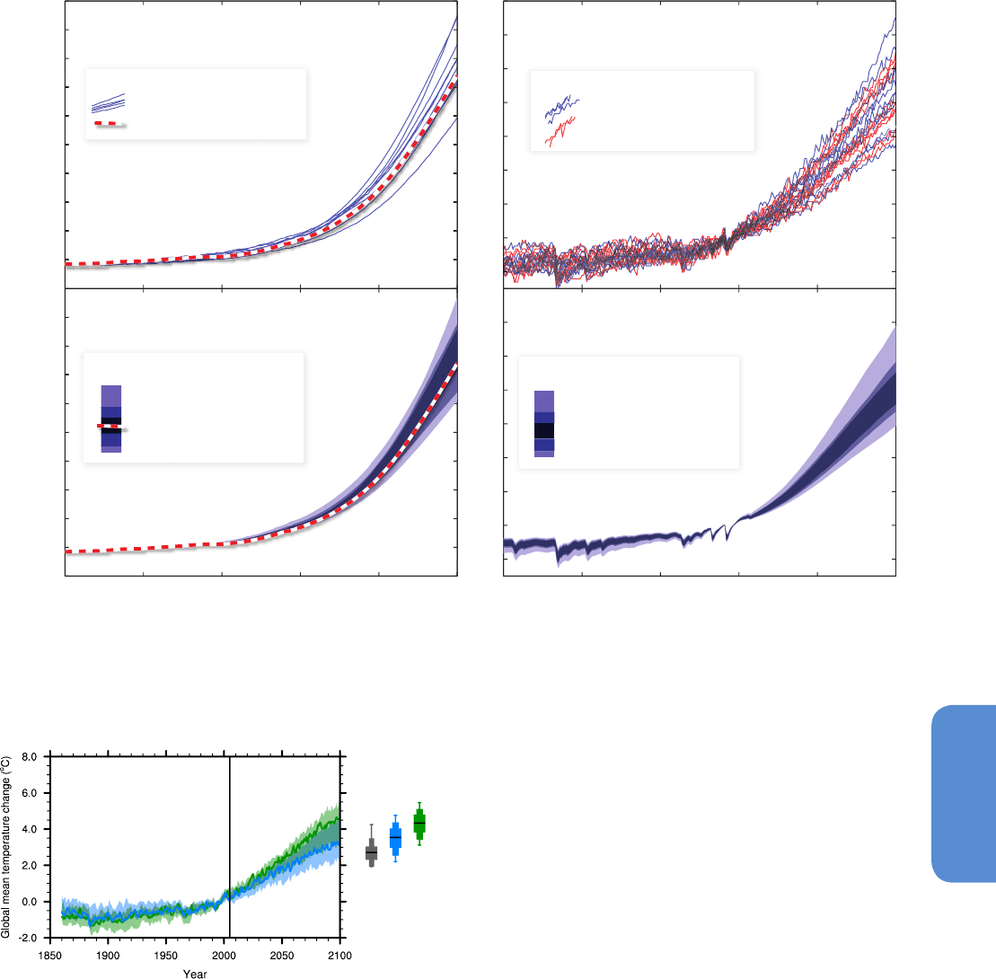
1097

Long-term Climate Change: Projections, Commitments and Irreversibility Chapter 12

there is medium conﬁdence in these numbers as are the ones on the

amount of carbon released (see Section 12.5.5.4) (MacDougall et al.,

2012; Schneider von Deimling et al., 2012).

12.4.8.2 Changes in Vegetation Cover

Vegetation cover can also be affected by climate change, with forest

cover potentially being decreasing (e.g., in the tropics) or increasing

(e.g., in high latitudes). In particular, the Amazon forest has been

the subject of several studies, generally agreeing that future climate

change would increase the risk tropical Amazon forest being replaced

by seasonal forest or even savannah (Huntingford et al., 2008; Jones

et al., 2009; Malhi et al., 2009). Increase in atmospheric CO

would

partly reduce such risk, through increase in water efﬁciency under ele-

vated CO

(Lapola et al., 2009; Malhi et al., 2009). Recent multi-model

estimates based on different CMIP3 climate scenarios and different

dynamic global vegetation models predict a moderate risk of tropical

forest reduction in South America and even lower risk for African and

Asian tropical forests (see also Section 12.5.5.6) (Gumpenberger et al.,

2010; Huntingford et al., 2013).

200

300

400

500

600

700

800

900

1000

1100

1200

concentration (ppm)

a Atmospheric CO

concentration

c Atmospheric CO

concentration

−1

b Global mean surface air temperature

d Global mean surface air temperature

1850 1900 1950 2000 2050 2100

200

300

400

500

600

700

800

900

1000

1100

1850 1900 1950 2000 2050 2100

−1

Global−Mean Temperature relative to 1986−2005 (°C)

CMIP3 & C4MIP emulation:

CMIP5:

CMIP3 & C4MIP emulation:

90%

68%

50%

Ranges

Concentration-driven default

90%

68%

50%

Ranges

Concentration-driven default

Emission-driven

Concentration-driven

Figure 12.36 | Simulated changes in (a) atmospheric CO

concentration and (b) global averaged surface temperature (°C) as calculated by the CMIP5 Earth System Models (ESMs)

for the RCP8.5 scenario when CO

emissions are prescribed to the ESMs as external forcing (blue). Also shown (b, in red) is the simulated warming from the same ESMs when directly

forced by atmospheric CO

concentration (a, red white line). Panels (c) and (d) show the range of CO

concentrations and global average surface temperature change simulated by

the Model for the Assessment of Greenhouse Gas-Induced Climate Change 6 (MAGICC6) simple climate model when emulating the CMIP3 models climate sensitivity range and the

Coupled Climate Carbon Cycle Model Intercomparison Project (C

MIP) models carbon cycle feedbacks. The default line in (c) is identical to the one in (a).

Figure 12.37 | Uncertainty in global mean temperature from Met Ofﬁce Hadley Centre

climate prediction model 3 (HadCM3) results exploring atmospheric physics and ter-

restrial carbon cycle parameter perturbations under the SRES A1B scenario (Murphy et

al., 2004; Booth et al., 2012). Relative uncertainties in the Perturbed Carbon Cycle (PCC,

green plume) and Perturbed Atmospheric Processes (PAP, blue plume) on global mean

anomalies of temperature (relative to the 1986–2005 period). The standard simulations

from the two ensembles, HadCM3 (blue solid) and HadCM3C (green solid) are also

shown. Three bars are shown on the right illustrating the 2100 temperature anomalies

associated with the CMIP3/AR4 ensemble (black) the PAP ensemble (blue) and PCC

ensemble (green). The ranges indicate the full range, 10th to 90th, 25th to 75th and

50th percentiles.

CMIP3

PAP

PCC

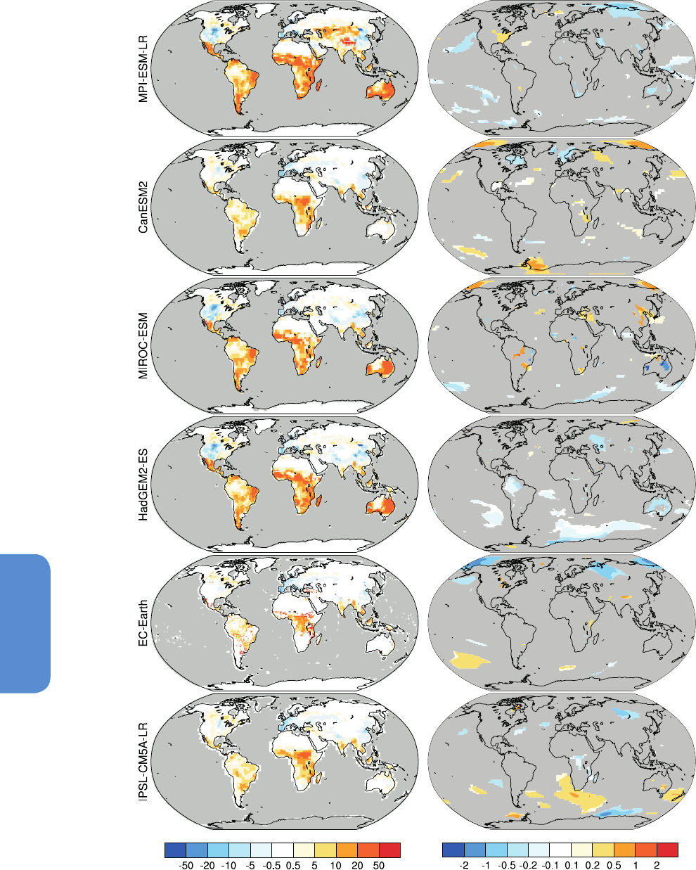
1098

Chapter 12 Long-term Climate Change: Projections, Commitments and Irreversibility

Figure 12.38 | Impact of land use change on surface temperature. LUCID-CMIP5 experiments where six ESMs were forced either with or without land use change beyond 2005

under the RCP8.5 scenario. Left maps of changes in total crop and pasture fraction (%) in the RCP8.5 simulations between 2006 and 2100 as implemented in each ESM.Right maps

show the differences in surface air temperature (averaged over the 2071–2100 period) between the simulations with and without land use change beyond 2005. Only statistically

signiﬁcant changes (p < 0.05) are shown.

Difference in crop and pasture fraction (%) Change in surface air temperature (°C)

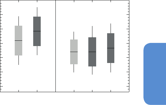
1099

Long-term Climate Change: Projections, Commitments and Irreversibility Chapter 12

ESMs simulations with interactive vegetation conﬁrmed known bio-

physical feedback associated with large-scale changes in vegetation.

In the northern high latitudes, warming-induced vegetation expansion

reduces surface albedo, enhancing the warming over these regions

(Falloon et al., 2012; Port et al., 2012), with potentially larger ampli-

ﬁcation due to ocean and sea ice response (Swann et al., 2010). Over

tropical forest, reduction of forest coverage would reduce evapotran-

spiration, also leading to a regional warming (Falloon et al., 2012; Port

et al., 2012).

CMIP5 ESMs also include human induced land cover changes (deforest-

ation, reforestation) affecting the climate system through changes in

land surface physical properties (Hurtt et al., 2011). Future changes

in land cover will have an impact on the climate system through bio-

physical and biogeochemical processes (e.g., Pongratz et al., 2010).

Biophysical processes include changes in surface albedo and changes

in partitioning between latent and sensible heat, while biogeochemi-

cal feedbacks essentially include change in CO

sources and sinks but

could potentially also include changes in N

O or CH

emissions. The bio-

physical response to future land cover changes has been investigated

within the SRES scenarios. Using the SRES A2 2100 land cover, Davin et

al. (2007) simulated a global cooling of 0.14 K relatively to a simulation

with present-day land cover, the cooling being largely driven by change

in albedo. Regional analyses have been performed in order to quantify

the biophysical impact of biofuels plantation generally ﬁnding a local

to regional cooling when annual crops are replaced by bioenergy crops,

such as sugar cane (Georgescu et al., 2011; Loarie et al., 2011). How-

ever, some energy crops require nitrogen inputs for their production,

leading inevitably to nitrous oxide (N

O) emissions, potentially reduc-

ing the direct cooling effect and the beneﬁt of biofuels as an alterna-

tive to fossil fuel emissions. Such emission estimates are still uncertain,

varying strongly for different crops, management methods, soil types

and reference systems (St. Clair et al., 2008; Smeets et al., 2009).

In the context of the Land-Use and Climate, IDentiﬁcation of robust

impacts (LUCID) project (Pitman et al., 2009) ESMs performed addi-

tional CMIP5 simulations in order to separate the biophysical from

the biogeochemical effects of land use changes in the RCP scenarios.

The LUCID–CMIP5 experiments were designed to complement RCP8.5

and RCP2.6 simulations of CMIP5, both of which showing an intensi-

ﬁcation of land use change over the 21st century. The LUCID–CMIP5

analysis was focussed on a difference in climate and land-atmosphere

ﬂuxes between the average of ensemble of simulations with and with-

out land use changes by the end of 21st century (Brovkin et al., 2013).

Due to different interpretation of land use classes, areas of crops and

pastures were speciﬁc for each ESM (Figure 12.38, left). On the global

scale, simulated biophysical effects of land use changes projected in

the CMIP5 experiments with prescribed CO

concentrations were not

signiﬁcant. However, these effects were signiﬁcant for regions with

land use changes >10%. Only three out of six participating models,

CanESM2, HadGEM2-ES and MIROC-ESM, reveal statistically signiﬁ-

cant changes in regional mean annual mean surface air temperature

for the RCP8.5 scenario (Figure 12.38, right). However, there is low

conﬁdence on the overall effect as there is no agreement among the

models on the sign of the global average temperature change due

to the biophysical effects of land use changes (Brovkin et al., 2013).

Changes in land surface albedo, available energy, latent and sensible

heat ﬂuxes were relatively small but signiﬁcant in most of ESMs for

regions with substantial land use changes. The scale of climatic effects

reﬂects a small magnitude of land use changes in both the RCP2.6 and

8.5 scenarios and their limitation mainly to the tropical and subtropical

regions where differences between biophysical effects of forests and

grasslands are less pronounced than in mid- and high latitudes. LUCID-

CMIP5 did not perform similar simulations for the RCP4.5 or RCP6.0

scenarios. As these two scenarios show a global decrease of land use

area, one might expect their climatic impact to be different from the

one seen in the RC2.6 and RCP8.5.

12.4.9 Consistency and Main Differences Between

Coupled Model Intercomparison Project Phase 3/

Coupled Model Intercomparison Project Phase 5

and Special Report on Emission Scenarios/

Representative Concentration Pathways

In the experiments collected under CMIP5, both models and scenario

have changed with respect to CMIP3 making a comparison with earlier

results and the scientiﬁc literature they generated (on which some of

this chapter’s content is still based) complex. The set of models used

in AR4 (the CMIP3 models) have been superseded by the new CMIP5

models (Table 12.1; Chapter 9) and the SRES scenarios have been

replaced by four RCPs (Section 12.3.1). In addition, the baseline period

used to compute anomalies has advanced 6 years, from 1980–1999 to

1986–2005.

SRES A1B

2080–2099 - 1980–1999

RCP6.0

2081–2100 - 1986–2005

Global mean temperature anomaly (°C)

4.0

3.5

3.0

2.5

2.0

1.5

1.0

CMIP3 CMIP5 (em)

CMIP5+CMIP3 (em) CMIP5

Figure 12.39 | Global mean temperature anomalies at the end of the 21st century

from General Circulation Model (GCM) experiments and emulators comparing CMIP3/

CMIP5 responses under SRES A1B and RCP6.0. The boxes and whiskers indicate the

5th percentile, mean value – 1 standard deviation, mean, mean value + 1 standard

deviation and 95th percentile of the distributions. The ﬁrst box-and-whiskers on the

left is computed directly from the CMIP3 ensemble and corresponds to the numbers

quoted in AR4. The emulated SRES A1B projections (second from left) of CMIP5 are

obtained by the method of Good et al. (2011a) and are calculated for the period 2080-

2099 expressed with respect to the AR4 baseline period of 1980–1999. Because of the

method, the subset of CMIP5 that are emulated are restricted to those with pre-indus-

trial control, abrupt 4 × CO

, historical, RCP4.5 and RCP8.5 simulations. The emulated

RCP6.0 projections of CMIP3 (third from left, see also Figure 12.8) are from Knutti and

Sedláček (2013) obtained using the method of Meinshausen et al. (2011b; 2011c) and

are calculated for the slightly different future period 2081–2100 to be consistent with

the rest of this chapter, and are expressed with respect to the AR5 baseline period of

1986–2005. The box-and-whiskers fourth from the left are a graphical representation of

the numbers shown in Table 12.2. The ﬁnal box-and-whiskers on the right is a combina-

tion of CMIP5 model output and emulation of CMIP5 RCP6.0 numbers for those models

that did not run RCP6.0.

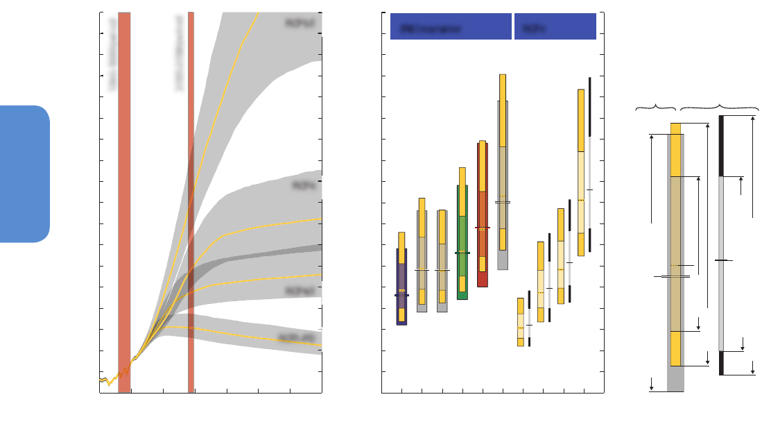
1100

Chapter 12 Long-term Climate Change: Projections, Commitments and Irreversibility

It would be extremely costly computationally to rerun the full CMIP3

ensemble under the new RCPs and/or the full CMIP5 ensemble under

the old SRES scenarios in order to separate model and scenario effects.

In the absence of a direct comparison, we rely on simpliﬁed model-

ling frameworks to emulate CMIP3/5 SRES/RCP model behaviour and

compare them. Figure 12.39 shows an emulation of the global mean

temperature response at the end of the 21st century that one would

expect from the CMIP5 models if they were run under SRES A1B. In this

case, anomalies are computed with respect to 1980–1999 for direct

comparison with the values reported in AR4 (Meehl et al., 2007b)

which used that baseline. The method used to emulate the SRES A1B

response of the CMIP5 is documented by Good et al. (2011a; 2013).

Ensemble-mean A1B RF was computed from CMIP3 projections using

the Forster and Taylor (2006) method, scaled to ensure consistency

with the forcing required by the method. The simple model is only used

to predict the temperature difference between A1B and RCP8.5, and

between A1B and RCP4.5 separately for each model. These differenc-

es are then added to CMIP5 GCM simulations of RCP8.5 and RCP4.5

respectively, and averaged to give a single A1B estimate. The emulated

CMIP5 SRES A1B results show a slightly larger mean response than the

actual CMIP3 models, with a similar spread (±1 standard deviation is

used in this case). The main reason for this is the slightly larger mean

transient climate response (TCR) in the subset of CMIP5 models avail-

able in comparison with the AR4 CMIP3 models. An alternative emula-

tion is presented by Knutti and Sedláček (2013) who use the simpliﬁed

MAGICC models with parameters chosen to emulate the response of

the CMIP3 models to RCP6.0 forcing, with anomalies expressed with

respect to the 1986–2005 baseline period (Figure 12.39). They too ﬁnd

a larger mean response in the CMIP5 case but also a larger spread (±1

standard deviation) in CMIP5. Uncertainties in the different approach-

es to emulating climate model simulations, for example estimating the

non-GHG RF, and the small sample sizes of CMIP3 and CMIP5 make

it difﬁcult to draw conclusions on the statistical signiﬁcance of the

differences displayed in Figure 12.39, but the same uncertainties lead

us to conclude that on the basis of these analyses there appears to

be no fundamental difference between the behaviour of the CMIP5

ensemble, in comparison with CMIP3.

Meinshausen et al. (2011a; 2011b) tuned MAGICC6 to emulate 19

GCMs from CMIP3. The results are temperature projections and their

uncertainties (based on the empirical distribution of the ensemble)

under each of the RCPs, extended to year 2500 (under constant emis-

sions for the lowest RCP and constant concentrations for the remain-

ing three). In the same paper, an ensemble produced by combining

carbon cycle parameter calibration to nine C

MIP models with the 19

CMIP3 model parameter calibrations is also used to estimate the emis-

sions implied by the various concentration pathways, had the CMIP3

models included a carbon cycle component. Rogelj et al. (2012) used

the same tool but performed a fully probabilistic analysis of the SRES

and RCP scenarios using a parameter space that is consistent with

SRESB1

SRESA1T

SRESB2

SRESA1B

SRESA2

SRESA1FI

RCP3-PD

RCP4.5

RCP6

RCP8.5

Temperature increase in 2090-2099 relative to 1980-1999 (°C)

1950 2000 2050 2100 2150 2200 2250 2300

Temperature increase relative to 1980-1999 (°C)

Temperature increase in 2090-2099 relative to pre-industrial (°C)

Temperature increase relative to pre-industrial (°C)

SRES scenarios RCPs

likely range (-40 to +60% around mean)

best estimate

median

66% range

90% range

median

90% range for emission-driven RCPs

66% range for emission-driven RCPs

IPCC AR4 values

Rogelj et al. (2012)

RCP3-PD

RCP4.5

RCP6

1980-1999 period

2090-2099 period

RCP8.5

Figure 12.40 | Temperature projections for SRES scenarios and the RCPs. (a) Time-evolving temperature distributions (66% range) for the four RCP scenarios computed with

the ECS distribution from Rogelj et al. (2012) and a model setup representing closely the carbon-cycle and climate system uncertainty estimates of the AR4 (grey areas). Median

paths are drawn in yellow. Red shaded areas indicate time periods referred to in panel b. (b) Ranges of estimated average temperature increase between 2090 and 2099 for SRES

scenarios and the RCPs respectively. Note that results are given both relative to 1980–1999 (left scale) and relative to pre-industrial (right scale). Yellow ranges indicate results

obtained by Rogelj et al. (2012). Colour-coding of AR4 ranges is chosen to be consistent with AR4 (Meehl et al., 2007b). RCP2.6 is labelled as RCP3-PD here.

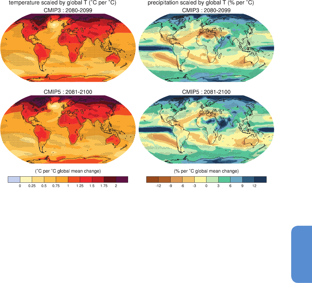
1101

Long-term Climate Change: Projections, Commitments and Irreversibility Chapter 12

CMIP3/C

MIP but a more general uncertainty characterization for key

quantities like equilibrium climate sensitivity, similarly to the approach

utilized by Meinshausen et al. (2009). Observational or other historical

constraints are also used in this study and the analysis is consistent

with the overall assessment of sources and ranges of uncertainties for

relevant quantities (equilibrium climate sensitivity above all) from AR4

(Meehl et al., 2007b , Box 10.2). Figure 12.40 summarizes results of this

probabilistic comparison for global temperature. The RCPs span a large

range of stabilization, mitigation and non-mitigation pathways and

the resulting range of temperature changes are larger than those pro-

duced under SRES scenarios, which do not consider mitigation options.

The SRES results span an interval between just above 1.0°C and 6.5°C

when considering the respective likely ranges of all scenarios, including

B1 as the lowest and A1FI as the highest. Emissions under RCP8.5 are

highest and the resulting temperature changes likely range from 4.0°C

to 6.1°C by 2100. The lowest RCP2.6 assumes signiﬁcant mitigation

and the global temperature change likely remains below 2°C.

Similar temperature change projections by the end of the 21st century

are obtained under RCP8.5 and SRES A1FI, RCP6 and SRES B2 and

RCP4.5 and SRES B1. There remain large differences though in the tran-

sient trajectories, with rates of change slower or faster for the different

pairs. These differences can be traced back to the interplay of the (neg-

ative) short-term effect of sulphate aerosols and the (positive) effect of

long-lived GHGs. Impact studies may be sensitive to the differences in

these temporal proﬁles so care should be taken in approximating SRES

with RCPs and vice versa.

While simple models can separate the effect of the scenarios and the

model response, no studies are currently available that allow an attri-

bution of the CMIP3-CMIP5 differences to changes in the transient

climate response, the carbon cycle, and the inclusion of new processes

(chemistry, land surface, vegetation). The fact that these sets of CMIP3

and CMIP5 experiments do not include emission-driven runs would

suggest that differences in the representation of the carbon cycle are

very unlikely to explain differences in the simulations, since the only

Figure 12.41 | Patterns of temperature (left column) and percent precipitation change (right column) for the CMIP3 models average (ﬁrst row) and CMIP5 models average (second

row), scaled by the corresponding global average temperature changes. The patterns are computed in both cases by taking the difference between the averages over the last 20

years of the 21st century experiments (2080–2099 for CMIP3 and 2081–2100 for CMIP5) and the last twenty years of the historic experiments (1980–1999 for CMIP3, 1986–2005

for CMIP5) and rescaling each difference by the corresponding change in global average temperature. This is done ﬁrst for each individual model, and then the results are averaged

across models. For the CMIP5 patterns, the RCP2.6 simulation of the FIO-ESM model was excluded because it did not show any warming by the end of the 21st century, thus not

complying with the method requirement that the pattern be estimated at a time when the temperature change signal from CO

increase has emerged. Stippling indicates a measure

of signiﬁcance of the difference between the two corresponding patterns obtained by a bootstrap exercise. Two subsets of the pooled set of CMIP3 and CMIP5 ensemble members

of the same size as the original ensembles, but without distinguishing CMIP3 from CMIP5 members, were randomly sampled 500 times. For each random sample we compute the

corresponding patterns and their difference, then the true difference is compared, grid-point by grid-point, to the distribution of the bootstrapped differences, and only grid-points

at which the value of the difference falls in the tails of the bootstrapped distribution (less than the 2.5 percentiles or the 97.5 percentiles) are stippled.

1102

Chapter 12 Long-term Climate Change: Projections, Commitments and Irreversibility

effect of changes in the carbon cycle representation would affect the

land surface, and thus would have only a minor effect on the climate

response at the global scale.

Figure 12.41 shows a comparison of the patterns of warming and

precipitation change from CMIP3 (using 23 models and three SRES

scenarios) and CMIP5 (using 46 models and four RCPs), utilizing the

pattern scaling methodology (Section 12.4.2). The geographic patterns

of mean change are very similar across the two ensembles of models,

with pattern correlations of 0.98 for temperature and 0.90 for precipi-

tation changes. However there exist signiﬁcant differences in the abso-

lute values of the patterns, if not in their geographic shapes. A simple

bootstrapping exercise that pooled together all models and scenari-

os and resampled 500 times the same numbers of models/scenarios

divided into two groups, but without distinguishing CMIP3 from CMIP5

(and thus SRES from RCPs) allows to compute a measure of signiﬁ-

cance of the actual differences in the patterns. Stippling in Figure 12.41

marks the large regions where the difference is signiﬁcant for temper-

ature and precipitation patterns. The temperature pattern from CMIP5

shows signiﬁcantly larger warming per degree Celsius of global mean

temperature change in the NH and less warming per degree Celsius in

the SH compared to the corresponding pattern from CMIP3. For precip-

itation patterns, CMIP5 shows signiﬁcantly larger increases per degree

Celsius in the NH and signiﬁcantly larger decreases per degree Celsius

in the SH compared to CMIP3. Even in this case we do not have studies

that allow tracing the source of these differences to speciﬁc changes in

models’ conﬁgurations, processes represented or scenarios run.

Knutti and Sedláček (2013) attempt to identify or rule out at least

some of these sources. Differences in model projections spread or its

counterpart, robustness, between CMIP3 and CMIP5 are discussed,

and it is shown that by comparing the behaviour of only a subset

of 11 models, contributed to the two CMIPs by the same group of

institutions, the robustness of CMIP5 versus that of CMIP3 actually

decreases slightly. This would suggest that the enhanced robustness

of CMIP5 is not clearly attributable to advances in modelling, and may

be a result of the fact that the CMIP5 ensemble contains different

versions of the same model that are counted as independent in this

measure of robustness.

A comparison of CMIP3 and CMIP5 results for extreme indices is pro-

vided in Sections 12.4.3.3 and Figure 12.13 for temperature extremes,

and Section 12.4.5.5 and Figure 12.26 for extremes in the water cycle.

12.5 Climate Change Beyond 2100,

Commitment, Stabilization and

Irreversibility

This section discusses the long term (century to millennia) climate

change based on the RCP scenario extensions and idealized scenari-

os, the commitment from current atmospheric composition and from

past emissions, the concept of cumulative carbon and the resulting

constraints on emissions for various temperature targets. The term

irreversibility is used in various ways in the literature. This report deﬁnes

a perturbed state as irreversible on a given time scale if the recov-

ery time scale from this state due to natural processes is signiﬁcantly

longer than the time it takes for the system to reach this perturbed

state (see Glossary), for example, the climate change resulting from

the long residence time of a CO

perturbation in the atmosphere. These

results are discussed in Sections 12.5.2 to 12.5.4. Aspects of irreversi-

bility in the context of abrupt change, multiple steady states and hys-

teresis are discussed in Section 12.5.5 and in Chapter 13 for ice sheets

and sea level rise.

12.5.1 Representative Concentration Pathway Extensions

The CMIP5 intercomparison project includes simulations extending the

four RCP scenarios to the year 2300 (see Section 12.3.1). This allows

exploring the longer-term climate response to idealized GHG and aer-

osols forcings (Meinshausen et al., 2011c). Continuing GHG emissions

beyond 2100 as in the RCP8.5 extension induces a total RF above 12

W m

–2

by 2300, while sustaining negative emissions beyond 2100, as

in the RCP2.6 extension, induces a total RF below 2 W m

–2

by 2300.

The projected warming for 2281–2300, relative to 1986–2005, is 0.6°C

(range 0.0°C to 1.2°C) for RCP2.6, 2.5°C (range 1.5°C to 3.5°C) for

RCP4.5, and 7.8°C (range 3.0°C to 12.6°C) for RCP8.5 (medium conﬁ-

dence, based on a limited number of CMIP5 simulations) (Figures 12.3

and 12.5, Table 12.2).

EMICs simulations have been performed following the same CMIP5

protocol for the historical simulation and RCP scenarios extended

to 2300 (Zickfeld et al., 2013). These scenarios have been prolonged

beyond 2300 to investigate longer-term commitment and irreversibility

(see below). Up to 2300, projected warming and the reduction of the

AMOC as simulated by the EMICs are similar to those simulated by the

CMIP5 ESMs (Figures 12.5 and 12.42).

12.5.2 Climate Change Commitment

Climate change commitment, the fact that the climate will change

further after the forcing or emissions have been eliminated or held

constant, has attracted increased attention by scientists and poli-

cymakers shortly before the completion of IPCC AR4 (Hansen et al.,

2005a; Meehl et al., 2005b, 2006; Wigley, 2005) (see also AR4 Section

10.7.1). However, the argument that the surface response would lag

the RF due to the large thermal reservoir of the ocean in fact goes back

much longer (Bryan et al., 1982; Hansen et al., 1984, 1985; Siegenthal-

er and Oeschger, 1984; Schlesinger, 1986; Mitchell et al., 2000; Weth-

erald et al., 2001). The discussion in this section is framed largely in

terms of temperature change, but other changes in the climate system

(e.g., precipitation) are closely related to changes in temperature (see

Sections 12.4.1.1 and 12.4.2). A summary of how past emissions relate

to future warming is also given in FAQ 12.3.

The Earth system has multiple response time scales related to different

thermal reservoirs (see also Section 12.5.3). For a step change in forcing

(instantaneous increase in the magnitude of the forcing and constant

forcing after that), a large fraction of the total of the surface tempera-

ture response will be realized within years to a few decades (Brasseur

and Roeckner, 2005; Knutti et al., 2008a; Murphy et al., 2009; Hansen et

al., 2011). The remaining response, realized over centuries, is controlled

by the slow mixing of the energy perturbation into the ocean (Stouffer,

2004). The response time scale depends on the amount of ocean mixing

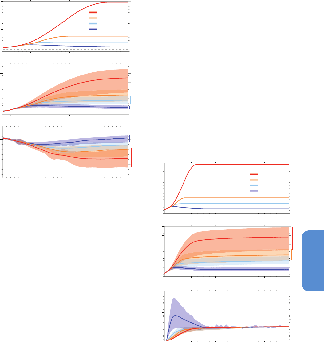
1103

Long-term Climate Change: Projections, Commitments and Irreversibility Chapter 12

and the strength of climate feedbacks, and is longer for higher climate

sensitivity (Hansen et al., 1985; Knutti et al., 2005). The transient cli-

mate response is therefore smaller than the equilibrium response, in

particular for high climate sensitivities. This can also be interpreted as

the ocean heat uptake being a negative feedback (Dufresne and Bony,

2008; Gregory and Forster, 2008). Delayed responses can also occur

due to processes other than ocean warming, for example, vegetation

change (Jones et al., 2009) or ice sheet melt that continues long after

the forcing has been stabilized (see Section 12.5.3).

Several forms of commitment are often discussed in the literature. The

most common is the ‘constant composition commitment’, the warm-

ing that would occur after stabilizing all radiative constituents at a

given year (for example year 2000) levels. For year 2000 commitment,

AOGCMs estimated a most likely value of about 0.6°C for 2100 (rel-

ative to 1980–1999, AR4 Section 10.7.1). A present-day composition

commitment simulation is not part of CMIP5, so direct comparison

with CMIP3 is not possible. However, the available CMIP5 results

based on the RCP4.5 extension with constant RF (see Section 12.5.1)

are consistent with those numbers, with an additional warming of

about 0.5°C 200 years after stabilization of the forcing (Figures 12.5

and 12.42).

500

1000

1500

2000

2100 2150 2200 2250

500

1000

1500

2000

(ppmv)

2000 2050 2300

RCP 2.6

RCP 4.5

RCP 6.0

RCP 8.5

(

Year

(Sv)

2100 2150 2200 22502000 2050 2300

Atmospheric CO

Surface air temperature change

Change in Atlantic meridional overturning circulation

-5

-10

-15

Figure 12.42 | (a) Atmospheric CO

, (b) projected global mean surface temperature

change and (c) projected change in the Atlantic meridional overturning circulation, as

simulated by EMICs for the four RCPs up to 2300 (Zickfeld et al., 2013). A 10-year

smoothing was applied. Shadings and bars denote the minimum to maximum range.

The dashed line on (a) indicates the pre-industrial CO

concentration.

A measure of constant composition commitment is the fraction of real-

ized warming which can be estimated as the ratio of the warming at a

given time to the long-term equilibrium warming (e.g., Stouffer, 2004;

Meehl et al., 2007b, Section 10.7.2; Eby et al., 2009; Solomon et al.,

2009). EMIC simulations have been performed with RCPs forcing up to

2300 prolonged until the end of the millennium with a constant forc-

ing set at the value reached by 2300 (Figure 12.43). When the forcing

stabilizes, the fraction of realized warming is signiﬁcantly below unity.

However, the fraction of realized warming depends on the history of

the forcing. For the RCP4.5 and RCP6.0 extension scenarios with early

stabilization, it is about 75% at the time of forcing stabilization; while

for RCP8.5, with stabilization occurring later, it is about 85% (see Figure

12.43); but for a 1% yr

–1

increase to 2 × CO

or 4 × CO

and con-

stant forcing thereafter, the fraction of realized warming is much small-

er, about 40 to 70% at the time when the forcing is kept constant. The

fraction of realized warming rises typically by 10% over the century

following the stabilization of forcing. Due to the long time scales in the

deep ocean, full equilibrium is reached only after hundreds to thou-

sands of years (Hansen et al., 1985; Gregory et al., 2004; Stouffer, 2004;

Meehl et al., 2007b, Section 10.7.2; Knutti et al., 2008a; Danabasoglu

and Gent, 2009; Held et al., 2010; Hansen et al., 2011; Li et al., 2013a).

500

1000

1500

2000

2000 2200 2400 2600 2800 3000

500

1000

1500

2000

(ppmv)

RCP 2.6

RCP 4.5

RCP 6.0

RCP 8.5

(

Year

Fraction of realized warming

Year

Atmospheric CO

Surface air temperature change

0.0

0.5

1.0

1.5

2.0

2.5

3.0

3.5

2000 2200 2400 2600 2800 3000

Figure 12.43 | (a) Atmospheric CO

, (b) projected global mean surface temperature

change and (c) fraction of realized warming calculated as the ratio of global tempera-

ture change at a given time to the change averaged over the 2980–2999 time period,

as simulated by Earth System Models of Intermediate Complexity (EMICs) for the 4

RCPs up to 2300 followed by a constant (year 2300 level) radiative forcing up to the

year 3000 (Zickfeld et al., 2013). A 10-year smoothing was applied. Shadings and bars

denote the minimum to maximum range. The dashed line on (a) indicates the pre-indus-

trial CO

concentration.

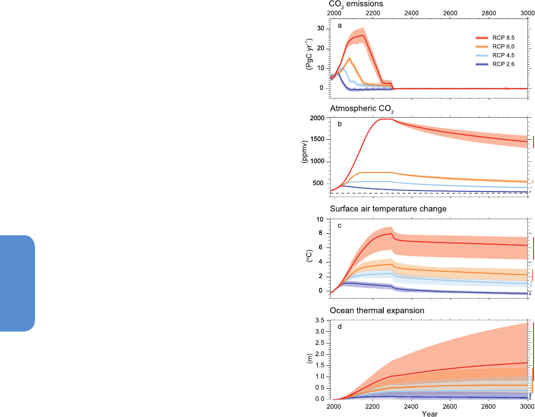
1104

Chapter 12 Long-term Climate Change: Projections, Commitments and Irreversibility

‘Constant emission commitment’ is the warming that would result

from maintaining annual anthropogenic emissions at the current level.

Few studies exist but it is estimated to be about 1°C to 2.5°C by 2100

assuming constant (year 2010) emissions in the future, based on the

MAGICC model calibrated to CMIP3 and C

MIP models (Meinshausen

et al., 2011a; Meinshausen et al., 2011b) (see FAQ 12.3). Such a scenar-

io is different from non-intervention economic scenarios, and it does not

stabilize global temperature, as any plausible emission path after 2100

would cause further warming. It is also different from a constant cumu-

lative emission scenario which implies zero emissions in the future.

Another form of commitment involves climate change when anthropo-

genic emissions are set to zero (‘zero emission commitment’). Results

from a variety of models ranging from EMICs (Meehl et al., 2007b;

Weaver et al., 2007; Matthews and Caldeira, 2008; Plattner et al.,

2008; Eby et al., 2009; Solomon et al., 2009; Friedlingstein et al., 2011)

to ESMs (Frölicher and Joos, 2010; Gillett et al., 2011; Gillett et al.,

2013) show that abruptly setting CO

emissions to zero (keeping other

forcings constant if accounted for) results in approximately constant

global temperature for several centuries onward. Those results indicate

that past emissions commit us to persistent warming for hundreds of

years, continuing at about the level of warming that has been realized.

On near equilibrium time scales of a few centuries to about a mil-

lennium, the temperature response to CO

emissions is controlled by

climate sensitivity (see Box 12.2) and the cumulative airborne fraction

of CO

over these time scales. After about a thousand years (i.e., near

thermal equilibrium) and cumulative CO

emissions less than about

2000 PgC, approximately 20 to 30% of the cumulative anthropogenic

carbon emissions still remain in the atmosphere (Montenegro et al.,

2007; Plattner et al., 2008; Archer et al., 2009; Frölicher and Joos, 2010;

Joos et al., 2013) (see Box 6.1) and maintain a substantial temperature

response long after emissions have ceased (Friedlingstein and Solo-

mon, 2005; Hare and Meinshausen, 2006; Weaver et al., 2007; Mat-

thews and Caldeira, 2008; Plattner et al., 2008; Eby et al., 2009; Lowe et

al., 2009; Solomon et al., 2009, 2010; Frölicher and Joos, 2010; Zickfeld

et al., 2012). In the transient phase, on a 100- to 1000-year time scale,

the approximately constant temperature results from a compensation

between delayed commitment warming (Meehl et al., 2005b; Wigley,

2005) and the reduction in atmospheric CO

resulting from ocean and

land carbon uptake as well as from the nonlinear dependence of RF on

atmospheric CO

(Meehl et al., 2007b; Plattner et al., 2008; Solomon

et al., 2009; Solomon et al., 2010). The commitment associated with

past emissions depends, as mentioned above, on the value of climate

sensitivity and cumulative CO

airborne fraction, but it also depends on

the choices made for other RF constituents. In a CO

only case and for

equilibrium climate sensitivities near 3°C, the warming commitment

(i.e., the warming relative to the time when emissions are stopped)

is near zero or slightly negative. For high climate sensitivities, and in

particular if aerosol emissions are eliminated at the same time, the

commitment from past emission can be signiﬁcantly positive, and is

a superposition of a fast response to reduced aerosols emissions and

a slow response associated with high climate sensitivities (Brasseur

and Roeckner, 2005; Hare and Meinshausen, 2006; Armour and Roe,

2011; Knutti and Plattner, 2012; Matthews and Zickfeld, 2012) (see

FAQ 12.3). In the real world, the emissions of CO

and non-CO

forcing

agents are of course coupled. All of the above studies support the con-

clusion that temperatures would decrease only very slowly (if at all),

even for strong reductions or complete elimination of CO

emissions,

and might even increase temporarily for an abrupt reduction of the

short-lived aerosols (FAQ 12.3). The implications of this fact for climate

stabilization are discussed in Section 12.5.4.

New EMIC simulations with pre-industrial CO

emissions and zero

non-CO

forcings after 2300 (Zickfeld et al., 2013) conﬁrm this behav-

iour (Figure 12.44) seen in many earlier studies (see above). Switching

off anthropogenic CO

emissions in 2300 leads to a continuous slow

decline of atmospheric CO

, to a signiﬁcantly slower decline of global

temperature and to a continuous increase in ocean thermal expansion

Figure 12.44 | (a) Compatible anthropogenic CO

emissions up to 2300, followed by

zero emissions after 2300, (b) prescribed atmospheric CO

concentration up to 2300

followed by projected CO

concentration after 2300, (c) global mean surface tempera-

ture change and (d) ocean thermal expansion as simulated by Earth System Models of

Intermediate Complexity (EMICs) for the four concentration driven RCPs with all forcings

included (Zickfeld et al., 2013). A 10-year smoothing was applied. The drop in tempera-

ture in 2300 is a result of eliminating all non-CO

forcings along with CO

emissions.

Shadings and bars denote the minimum to maximum range. The dashed line on (b)

indicates the pre-industrial CO

concentration.

1105

Long-term Climate Change: Projections, Commitments and Irreversibility Chapter 12

over the course of the millennium. Larger forcings induce longer delays

before the Earth system would reach equilibrium. For RCP8.5, by year

3000 (700 years after emissions have ceased) global temperature has

decreased only by 1°C to 2°C (relative to its peak value by 2300) and

ocean thermal expansion has almost doubled (relative to 2300) and is

still increasing (Zickfeld et al., 2013).

The previous paragraph discussed climate change commitment from

GHGs that have already been emitted. Another form of commitment

refers to climate change associated with heat and carbon that has

gone into the land surface and oceans. This would be relevant to the

consequences of a one-time removal of all of the excess CO

in the

atmosphere and is computed by taking a transient simulation and

instantaneously setting atmospheric CO

concentrations to initial

(pre-industrial) values (Cao and Caldeira, 2010). In such an extreme

case, there would be a net ﬂux of CO

from the ocean and land surface

to the atmosphere, releasing an amount of CO

representing about

30% of what was removed from the atmosphere, i.e., the airborne frac-

tion applies equally to positive and negative emissions, and it depends

on the emissions history. A related form of experiment investigates

the consequences of an initial complete removal followed by sustained

removal of any CO

returned to the atmosphere from the land sur-

face and oceans, and is computed by setting atmospheric CO

con-

centrations to pre-industrial values and maintaining this concentration

(Cao and Caldeira, 2010). In this case, only about one-tenth of the

pre-existing temperature perturbation persists for more than half of a

century. A similar study performed with a GFDL AOGCM where forcing

was instantaneously returned to its pre-industrial value, found larger

residual warming, up to 30% of the pre-existing warming (Held et al.,

2010).

Several studies on commitment to past emissions have demonstrat-

ed that the persistence of warming is substantially longer than the

lifetime of anthropogenic GHGs themselves, as a result of nonlinear

absorption effects as well as the slow heat transfer into and out of

the ocean. In much the same way as the warming to a step increase of

forcing is delayed, the cooling after setting RF to zero is also delayed.

Loss of excess heat from the ocean will lead to a positive surface air

temperature anomaly for decades to centuries (Held et al., 2010; Solo-

mon et al., 2010; Bouttes et al., 2013).

A more general form of commitment is the question of how much

warming we are committed to as a result of inertia and hence com-

mitments related to the time scales for energy system transitions and

other societal, economic and technological aspects (Grubb, 1997;

Washington et al., 2009; Davis et al., 2010). For example, Davis et al.

(2010) estimated climate commitment of 1.3°C (range 1.1°C to 1.4°C,

relative to pre-industrial) from existing CO

-emitting devices under

speciﬁc assumptions regarding their lifetimes. These forms of commit-

ment, however, are strongly based on political, economic and social

assumptions that are outside the domain of IPCC WGI and are not

further considered here.

12.5.3 Forcing and Response, Time Scales of Feedbacks

Equilibrium climate sensitivity (ECS), transient climate response

(TCR) and climate feedbacks are useful concepts to characterize the

response of a model to an external forcing perturbation. However,

there are limitations to the concept of RF (Joshi et al., 2003; Shine et

al., 2003; Hansen et al., 2005b; Stuber et al., 2005), and the separation

of forcings and fast (or rapid) responses (e.g., clouds changing almost

instantaneously as a result of CO

-induced heating rates rather than

as a response to the slower surface warming) is sometimes difﬁcult

(Andrews and Forster, 2008; Gregory and Webb, 2008). Equilibrium

warming also depends on the type of forcing (Stott et al., 2003; Hansen

et al., 2005b; Davin et al., 2007). ECS is time or state dependent in

some models (Senior and Mitchell, 2000; Gregory et al., 2004; Boer et

al., 2005; Williams et al., 2008; Colman and McAvaney, 2009; Colman

and Power, 2010), and in some but not all models climate sensitivity

from a slab ocean version differs from that of coupled models or the

effective climate sensitivity (see Glossary) diagnosed from a transient

coupled integration (Gregory et al., 2004; Danabasoglu and Gent,

2009; Li et al., 2013a). The computational cost of coupled AOGCMs is

often prohibitively large to run simulations to full equilibrium, and only

a few models have performed those (Manabe and Stouffer, 1994; Voss

and Mikolajewicz, 2001; Gregory et al., 2004; Danabasoglu and Gent,

2009; Li et al., 2013a). Because of the time dependence of effective

climate sensitivity, ﬁtting simple models to AOGCMs over the ﬁrst few

centuries may lead to errors when inferring the response on multi-cen-

tury time scales. In the HadCM3 case the long-term warming would be

underestimated by 30% if extrapolated from the ﬁrst century (Gregory

et al., 2004), in other models the warming of the slab and coupled

model is almost identical (Danabasoglu and Gent, 2009). The assump-

tion that the response to different forcings is approximately additive

appears to be justiﬁed for large-scale temperature changes but limited

for other climate variables (Boer and Yu, 2003; Sexton et al., 2003; Gil-

lett et al., 2004; Meehl et al., 2004; Jones et al., 2007). A more complete

discussion of the concept of ECS and the limitations is given in Knutti

and Hegerl (2008). The CMIP5 model estimates of ECS and TCR are

also discussed in Section 9.7. Despite all limitations, the ECS and TCR

remain key concepts to characterize the transient and near equilibrium

warming as a response to RF on time scales of centuries. Their overall

assessment is given in Box 12.2.

A number of recent studies suggest that equilibrium climate sensitiv-

ities determined from AOGCMs and recent warming trends may sig-

niﬁcantly underestimate the true Earth system sensitivity (see Glossa-

ry) which is realized when equilibration is reached on millennial time

scales (Hansen et al., 2008; Rohling et al., 2009; Lunt et al., 2010; Pagani

et al., 2010; Rohling and Members, 2012). The argument is that slow

feedbacks associated with vegetation changes and ice sheets have

their own intrinsic long time scales and are not represented in most

models (Jones et al., 2009). Additional feedbacks are mostly thought

to be positive but negative feedbacks of smaller magnitude are also

simulated (Swingedouw et al., 2008; Goelzer et al., 2011). The climate

sensitivity of a model may therefore not reﬂect the sensitivity of the

full Earth system because those feedback processes are not considered

(see also Sections 10.8, 5.3.1 and 5.3.3.2; Box 5.1). Feedbacks deter-

mined in very different base state (e.g., the Last Glacial Maximum)

differ from those in the current warm period (Rohling and Members,

2012), and relationships between observables and climate sensitiv-

ity are model dependent (Cruciﬁx, 2006; Schneider von Deimling et

al., 2006; Edwards et al., 2007; Hargreaves et al., 2007, 2012). Esti-

mates of climate sensitivity based on paleoclimate archives (Hansen

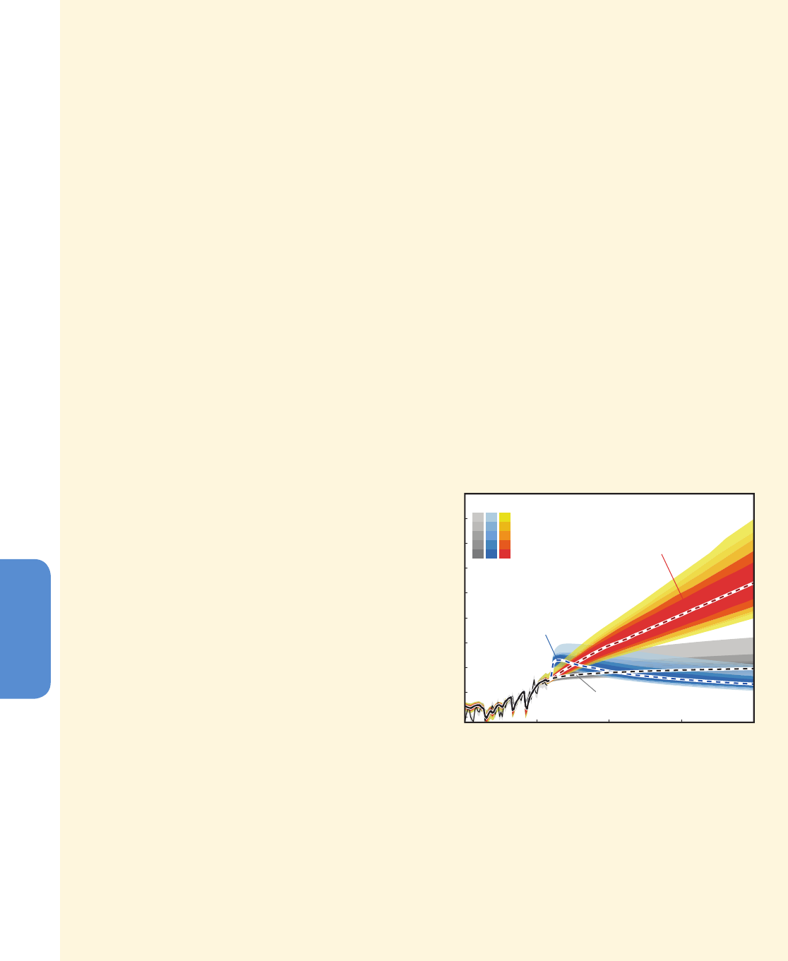
1106

Chapter 12 Long-term Climate Change: Projections, Commitments and Irreversibility

Frequently Asked Questions

FAQ 12.3 | What Would Happen to Future Climate if We Stopped Emissions Today?

Stopping emissions today is a scenario that is not plausible, but it is one of several idealized cases that provide

insight into the response of the climate system and carbon cycle. As a result of the multiple time scales in the climate

system, the relation between change in emissions and climate response is quite complex, with some changes still

occurring long after emissions ceased. Models and process understanding show that as a result of the large ocean

inertia and the long lifetime of many greenhouse gases, primarily carbon dioxide, much of the warming would

persist for centuries after greenhouse gas emissions have stopped.

When emitted in the atmosphere, greenhouse gases get removed through chemical reactions with other reactive

components or, in the case of carbon dioxide (CO

), get exchanged with the ocean and the land. These processes

characterize the lifetime of the gas in the atmosphere, deﬁned as the time it takes for a concentration pulse to

decrease by a factor of e (2.71). How long greenhouse gases and aerosols persist in the atmosphere varies over a

wide range, from days to thousands of years. For example, aerosols have a lifetime of weeks, methane (CH

) of

about 10 years, nitrous oxide (N

O) of about 100 years and hexaﬂuoroethane (C

) of about 10,000 years. CO

more complicated as it is removed from the atmosphere through multiple physical and biogeochemical processes in

the ocean and the land; all operating at different time scales. For an emission pulse of about 1000 PgC, about half

is removed within a few decades, but the remaining fraction stays in the atmosphere for much longer. About 15 to

40% of the CO

pulse is still in the atmosphere after 1000 years.

As a result of the signiﬁcant lifetimes of major anthropogenic greenhouse gases, the increased atmospheric concen-

tration due to past emissions will persist long after emissions are ceased. Concentration of greenhouse gases would

not return immediately to their pre-industrial levels if emissions were halted. Methane concentration would return

to values close to pre-industrial level in about 50 years, N

O concentrations would need several centuries, while

would essentially never come back to its pre-industrial level on time scales relevant for our society. Changes

in emissions of short-lived species like aerosols on the other hand would result in nearly instantaneous changes in

their concentrations.

The climate system response to the greenhouse gases

and aerosols forcing is characterized by an inertia,

driven mainly by the ocean. The ocean has a very large

capacity of absorbing heat and a slow mixing between

the surface and the deep ocean. This means that it will

take several centuries for the whole ocean to warm up

and to reach equilibrium with the altered radiative forc-

ing. The surface ocean (and hence the continents) will

continue to warm until it reaches a surface temperature

in equilibrium with this new radiative forcing. The AR4

showed that if concentration of greenhouse gases were

held constant at present day level, the Earth surface

would still continue to warm by about 0.6°C over the

21st century relative to the year 2000. This is the climate

commitment to current concentrations (or constant

composition commitment), shown in grey in FAQ 12.3,

Figure 1. Constant emissions at current levels would fur-

ther increase the atmospheric concentration and result

in much more warming than observed so far (FAQ 12.3,

Figure 1, red lines).

Even if anthropogenic greenhouses gas emissions were

halted now, the radiative forcing due to these long-

lived greenhouse gases concentrations would only

slowly decrease in the future, at a rate determined

by the lifetime of the gas (see above). Moreover, the

1950 2000 2050 2100 2150

Global surface warming (°C)

Year

90%

85%

80%

68%

50%

Constant Emissions

Zero Emissions

Constant Forcing

Ensemble Range:

FAQ 12.3, Figure 1 | Projections based on the energy balance carbon

cycle model Model for the Assessment of Greenhouse Gas-Induced Climate

Change (MAGICC) for constant atmospheric composition (constant forcing,

grey), constant emissions (red) and zero future emissions (blue) starting in

2010, with estimates of uncertainty. Figure adapted from Hare and Mein-

shausen (2006) based on the calibration of a simple carbon cycle climate

model to all Coupled Model Intercomparison Project Phase 3 (CMIP3) and

Coupled Climate Carbon Cycle Model Intercomparison Project (C4MIP)

models (Meinshausen et al., 2011a; Meinshausen et al., 2011b). Results are

based on a full transient simulation starting from pre-industrial and using

all radiative forcing components. The thin black line and shading denote the

observed warming and uncertainty.

(continued on next page)

1107

Long-term Climate Change: Projections, Commitments and Irreversibility Chapter 12

FAQ 12.3 (continued)

climate response of the Earth System to that radiative forcing would be even slower. Global temperature would

not respond quickly to the greenhouse gas concentration changes. Eliminating CO

emissions only would lead to

near constant temperature for many centuries. Eliminating short-lived negative forcings from sulphate aerosols at

the same time (e.g., by air pollution reduction measures) would cause a temporary warming of a few tenths of a

degree, as shown in blue in FAQ 12.3, Figure 1. Setting all emissions to zero would therefore, after a short warming,

lead to a near stabilization of the climate for multiple centuries. This is called the commitment from past emissions

(or zero future emission commitment). The concentration of GHG would decrease and hence the radiative forcing

as well, but the inertia of the climate system would delay the temperature response.

As a consequence of the large inertia in the climate and carbon cycle, the long-term global temperature is largely

controlled by total CO

emissions that have accumulated over time, irrespective of the time when they were emit-

ted. Limiting global warming below a given level (e.g., 2°C above pre-industrial) therefore implies a given budget

of CO

, that is, higher emissions earlier implies stronger reductions later. A higher climate target allows for a higher

concentration peak, and hence larger cumulative CO

emissions (e.g., permitting a delay in the necessary emis-

sion reduction).

Global temperature is a useful aggregate number to describe the magnitude of climate change, but not all changes

will scale linearly global temperature. Changes in the water cycle for example also depend on the type of forcing

(e.g., greenhouse gases, aerosols, land use change), slower components of the Earth system such as sea level rise

and ice sheet would take much longer to respond, and there may be critical thresholds or abrupt or irreversible

changes in the climate system.

et al., 2008; Rohling et al., 2009; Lunt et al., 2010; Pagani et al., 2010;

Schmittner et al., 2011; Rohling and Members, 2012), most but not all

based on climate states colder than present, are therefore not neces-

sarily representative for an estimate of climate sensitivity today (see

also Sections 5.3.1, 5.3.3.2, Box 5.1). Also it is uncertain on which time

scale some of those Earth system feedbacks would become signiﬁcant.

Equilibrium climate sensitivity undoubtedly remains a key quantity,

useful to relate a change in GHGs or other forcings to a global tempera-

ture change. But the above caveats imply that estimates based on past

climate states very different from today, estimates based on time scales

different than those relevant for climate stabilization (e.g., estimates

based on climate response to volcanic eruptions), or based on forcings

other than GHGs (e.g., spatially non-uniform land cover changes, vol-

canic eruptions or solar forcing) may differ from the climate sensitivity

measuring the climate feedbacks of the Earth system today, and this

measure, in turn, may be slightly different from the sensitivity of the

Earth in a much warmer state on time scales of millennia. The TCR and

the transient climate response to cumulative carbon emissions (TCRE)

are often more directly relevant to evaluate short term changes and

emission reductions needed for stabilization (see Section 12.5.4).

12.5.4 Climate Stabilization and Long-term Climate

Targets

This section discusses the relation between emissions and climate

targets, in the context of the uncertainties characterizing both the

transient and the equilibrium climate responses to emissions. ‘Climate

targets’ considered here are both stabilizing temperature at a speci-

ﬁed value and avoiding a warming beyond a predeﬁned threshold.

The latter idea of limiting peak warming is a more general concept

than stabilization of temperature or atmospheric CO

, and one that is

more realistic than an exact climate stabilization which would require

perpetual non-zero positive emissions to counteract the otherwise

unavoidable long-term slow decrease in global temperature (Matsuno

et al., 2012a) (Figure 12.44).

12.5.4.1 Background

The concept of stabilization is strongly linked to the ultimate objective

of the UNFCCC, which is ‘to achieve […] stabilization of greenhouse

gas concentrations in the atmosphere at a level that would prevent

dangerous anthropogenic interference with the climate system’. Recent

policy discussions focussed on a global temperature increase, rather

than on GHG concentrations. The most prominent target currently dis-

cussed is the 2°C temperature target, that is, to limit global temper-

ature increase relative to pre-industrial times to below 2°C. The 2°C

target has been used ﬁrst by the European Union as a policy target in

1996 but can be traced further back (Jaeger and Jaeger, 2010; Randalls,

2010). Climate impacts however are geographically diverse (Joshi et

al., 2011) and sector speciﬁc, and no objective threshold deﬁnes when

dangerous interference is reached. Some changes may be delayed or

irreversible, and some impacts are likely to be beneﬁcial. It is thus not

possible to deﬁne a single critical threshold without value judgments

and without assumptions on how to aggregate current and future

costs and beneﬁts. Targets other than 2°C have been proposed (e.g.,

1.5°C global warming relative to pre-industrial), or targets based on

concentration levels, for example, 350 ppm (Hansen et al., 2008).

The rate of change may also be important (e.g., for adaptation). This

section does not advocate or defend any threshold, nor does it judge

1108

Chapter 12 Long-term Climate Change: Projections, Commitments and Irreversibility

the economic or political feasibility of such goals, but simply assess-

es the implications of different illustrative climate targets on allowed

carbon emissions, based on our current understanding of climate and

carbon cycle feedbacks.

12.5.4.2 Constraints on Cumulative Carbon Emissions

The current RF from GHGs maintained indeﬁnitely (i.e., the commit-

ment from constant greenhouse gas concentrations) would correspond

to approximately 2°C warming. That, however, does not imply that the

commitment from past emissions has already exceeded 2°C. Part of the

positive RF from GHGs is currently compensated by negative aerosol

forcing, and stopping GHG emissions would lead to a decrease in the

GHG forcing. Actively removing CO

from the atmosphere, for example

by the combined use of biomass energy and carbon capture and stor-

age, would further accelerate the decrease in GHG forcing.

The total amount of anthropogenic CO

released in the atmosphere

(often termed cumulative carbon emission) is a good indicator of the

atmospheric CO

concentration and hence of the global warming

response to CO

. The ratio of global temperature change to total cumu-

lative anthropogenic CO

emissions (TCRE) is relatively constant over

time and independent of the scenario, but is model dependent as it

depends on the model cumulative airborne fraction of CO

and ECS/

TCR (Matthews and Caldeira, 2008; Allen et al., 2009; Gregory et al.,

2009; Matthews et al., 2009; Meinshausen et al., 2009; Zickfeld et al.,

2009; Bowerman et al., 2011; Knutti and Plattner, 2012; Zickfeld et al.,

2012, 2013). This is consistent with an earlier study indicating that

the global warming potential of CO

is approximately independent of

the scenario (Caldeira and Kasting, 1993). The concept of a constant

ratio of cumulative emissions of CO

to temperature holds well only

until temperatures peak (see Figure 12.45e) and only for smoothly var-

ying cumulative CO

emissions (Gillett et al., 2013). It does not hold

for stabilization on millennial time scales or for non-CO

forcings, and

there is limited evidence for its applicability for cumulative emissions

exceeding 2000 PgC owing to limited simulations available (Plattner et

al., 2008; Hajima et al., 2012; Matsuno et al., 2012b; Gillett et al., 2013;

Zickfeld et al., 2013). For non-CO

forcings with shorter atmospheric

life times than CO

the rate of emissions at the time of peak warming

is more important than the cumulative emissions over time (Smith et

al., 2012).

Assuming constant climate sensitivity and ﬁxed carbon cycle feed-

backs, long-term (several centuries to millennium) stabilization of

global temperatures requires eventually the stabilization of atmos-

pheric concentrations (or decreasing concentrations if the temperature

should be stabilized more quickly). This requires decreasing emissions

to near-zero (Jones et al., 2006; Meehl et al., 2007b; Weaver et al.,

2007; Matthews and Caldeira, 2008; Plattner et al., 2008; Allen et al.,

2009; Matthews et al., 2009; Meinshausen et al., 2009; Zickfeld et al.,

2009; Friedlingstein et al., 2011; Gillett et al., 2011; Roeckner et al.,

2011; Knutti and Plattner, 2012; Matsuno et al., 2012a).

The relationships between cumulative emissions and temperature for

various studies are shown in Figure 12.45. Note that some lines mark

the evolution of temperature as a function of emissions over time

while other panels show peak temperatures for different simulations.

Also some models prescribe only CO

emissions while others use multi

gas scenarios, and the time horizons differ. The warming is usually

larger if non-CO

forcings are considered, since the net effect of the

non-CO

forcings is positive in most scenarios (Hajima et al., 2012). Not

all numbers are therefore directly comparable. Matthews et al. (2009)

estimated the TCRE as 1°C to 2.1°C per 1000 PgC (TtC, or 10

metric

tonnes of carbon) (5 to 95%) based on the C

MIP model range (Figure

12.45a). The ENSEMBLES E1 show a range of 1°C to 4°C per 1000 PgC

(scaled from 0.5°C to 2°C for 500 PgC, Figure 12.45d) (Johns et al.,

2011). Rogelj et al. (2012) estimate a 5 to 95% range of about 1°C to

2°C per 1000 PgC (Figure 12.45e) based on the MAGICC model cali-

brated to the C

MIP model range and the likely range of 2°C to 4.5°C

for climate sensitivity given in AR4. Allen et al. (2009) used a simple

model and found 1.3°C to 3.9°C per 1000 PgC (5 to 95%) for peak

warming (Figure 12.45g) and 1.4°C to 2.5°C for TCRE. The EMICs TCRE

simulations suggest a range of about 1.4°C to 2.5°C per 1000 PgC and

a mean of 1.9°C per 1000 PgC (Zickfeld et al., 2013) (Figure 12.45h).

The results of Meinshausen et al. (2009) conﬁrm the approximate lin-

earity between temperature and CO

emissions (Figure 12.45b). Their

results are difﬁcult to compare owing to the shorter time period con-

sidered, but the model was found to be consistent with that of Allen et

al. (2009). Zickfeld et al. (2009), using an EMIC, ﬁnd a best estimate of

about 1.5°C per 1000 PgC. Gillett et al. (2013) ﬁnd a range of 0.8°C to

2.4°C per 1000 PgC in 15 CMIP5 models and derive an observationally

constrained range of 0.7°C to 2.0°C per 1000 PgC. Results from much

earlier model studies support the near linear relationship of cumulative

emissions and global temperature, even though these studies did not

discuss the linear relationship. An example is given in Figure 12.45c

based on data shown in IPCC TAR Figure 13.3 (IPCC, 2001) and IPCC

AR4 Figure 10.35 (Meehl et al., 2007b). The relationships between

cumulative CO

emissions and temperature in CMIP5 are shown in

Figure 12.45f for the 1% yr

–1

increase scenarios and in Figure

12.45i for the RCP8.5 emission driven ESM simulations (Gillett et al.,

2013). Compatible emissions from concentration driven CMIP5 ESMs

are discussed in Section 6.4.3.3.

Expert judgement based on the available evidence therefore suggests

that the TCRE is likely between 0.8°C to 2.5°C per 1000 PgC, for cumu-

lative CO

emissions less than about 2000 PgC until the time at which

temperature peaks. Under these conditions, and for low to medium

estimates of climate sensitivity, the TCRE is nearly identical to the peak

climate response to cumulative carbon emissions. For high climate

sensitivity, strong carbon cycle climate feedbacks or large cumulative

emissions, the peak warming can be delayed and the peak response

may be different from TCRE, but is often poorly constrained by models

and observations. The range of TCRE assessed here is consistent with

other recent attempts to synthesize the available evidence (NRC, 2011;

Matthews et al., 2012). The results by Schwartz et al. (2010, 2012)

imply a much larger warming for the carbon emitted over the historical

period and have been questioned by Knutti and Plattner (2012) for

neglecting the relevant response time scales and combining a transient

airborne fraction with an equilibrium climate sensitivity.

The TCRE can be compared to the temperature response to emissions

on a time scale of about 1000 years after emissions cease. This can

be estimated from the likely range of equilibrium climate sensitivity

(1.5°C to 4.5°C) and a cumulative CO

airborne fraction after about

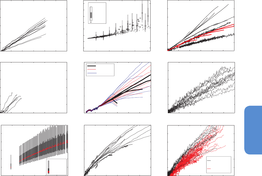
1109

Long-term Climate Change: Projections, Commitments and Irreversibility Chapter 12

1000 years of about 25 ± 5% (Archer et al., 2009; Joos et al., 2013).

Again combining the extreme values would suggest a range of 0.6°C

to 2.7°C per 1000 PgC, and 1.5°C per 1000 PgC for an ECS of 3°C

and a cumulative airborne fraction of 25%. However, this equilibrium

estimate is based on feedbacks estimated for the present day climate.

Climate and carbon cycle feedbacks may increase substantially on long

time scales and for high cumulative CO

emissions (see Section 12.5.3),

introducing large uncertainties in particular on the upper bound. Based

on paleoclimate data and an analytical model, Goodwin et al. (2009)

estimate a long term RF of 1.5 W m

–2

for an emission of 1000 PgC. For

an equilibrium climate sensitivity of 3°C this corresponds to a warming

of 1.2°C on millennial time scales, consistent with the climate carbon

cycle models results discussed above.

The uncertainty in TCRE is caused by the uncertainty in the physical

feedbacks and ocean heat uptake (reﬂected in TCR) and uncertainties

in carbon cycle feedbacks (affecting the cumulative airborne fraction

of CO

). TCRE only characterizes the warming due to CO

emissions,

and contributions from non-CO

gases need to be considered sepa-

rately when estimating likelihoods to stay below a temperature limit.

Warming as a function of cumulative CO

emissions is similar in the

four RCP scenarios, and larger than that due to CO

alone, since non-

forcings contribute warming in these scenarios (compare Figure

12.45 f, i) (Hajima et al., 2012).

0 500 1000 1500 2000 2500 3000

Cumulative CO

emissions (PgC)

Transient temperature increase

(°C) (rel. to 1850-1875)

0 500 1000 1500 2000 2500 3000

Cumulative CO

emissions (PgC)

Transient temperature increase

(°C) (rel. to 1865-1875)

0 500 1000 1500 2000 2500 3000

Cumulative CO

emissions (PgC)

Transient temperature increase

(°C) (rel. to 1850-1875)

0 500 1000 1500 2000 2500 3000

Cumulative CO

eq emissions (PgC-eq)

Transient temperature increase

(°C) (rel. to 1850-1875)

Median

66% range

90% range

500 1000 1500 2000 2500 3000

Cumulative CO

emissions to 2200 (PgC)

Peak CO

induced warming

(°C) (rel. to per-industrial)

0 500 1000 1500 2000 2500 3000

Cumulative diagnosed CO

emissions (PgC)

Transient temperature increase

(°C) (rel. to 1850-1875)

0 500 1000 1500 2000 2500 3000

Cumulative CO

emissions (PgC)

Transient temperature increase

(°C) (rel. to yr 0)

Very likely

Likely

Most likely

1000 1500 2000 2500 3000 3500

Cumulative Kyoto-gas emissions 2000-2049 (PgCO

-eq)

Global mean air surface temperature

(°C) (rel. to 1860-1899)

90%

68%

Medians

Ranges:

0 500 1000 1500 2000 2500 3000

Cumulative diagnosed CO

emissions (PgC)

Transient temperature increase

(°C) (rel. to 1860-1880)

FF & industry

(emis-driven)

Total (back-

calculated)

Figure 12.45 | Global temperature change vs. cumulative carbon emissions for different scenarios and models. (a) Transient global temperature increase vs. cumulative CO

emis-

sions for Coupled Climate Carbon Cycle Model Intercomparison Project (C

MIP) (Matthews et al., 2009). (b) Maximum temperature increase until 2100 vs. cumulative Kyoto-gas

emissions (CO

equivalent; note that all other panels are given in C equivalent) (Meinshausen et al., 2009). (c) Transient temperature increase vs. cumulative CO

emissions for IPCC

TAR models (red, IPCC TAR Figure 13.3) and IPCC AR4 Earth System Models of Intermediate Complexity (EMICs, black: IPCC AR4 Figure 10.35). (d) As in (a) but for the ENSEMBLES

E1 scenario (Johns et al., 2011). (e) Transient temperature increase for the RCP scenarios based on the Model for the Assessment of Greenhouse Gas-Induced Climate Change

(MAGICC) model constrained to C

MIP, observed warming, and the IPCC AR4 climate sensitivity range (Rogelj et al., 2012). (f) Transient temperature change from the CMIP5 1%

–1

concentration driven simulations. (g) Peak CO

induced warming vs. cumulative CO

emissions to 2200 (Allen et al., 2009; Bowerman et al., 2011). (h) Transient temperature

increase from the new EMIC RCP simulations (Zickfeld et al., 2013). (i) Transient temperature change from the CMIP5 historical and RCP8.5 emission driven simulations (black) and

transient temperature change in all concentration-driven CMIP5 RCP simulations with back-calculated emissions (red). Note that black lines in panel (i) do not include land use CO

and that warming in (i) is higher than in (f) due to additional non-CO

forcings.

1110

Chapter 12 Long-term Climate Change: Projections, Commitments and Irreversibility

Box 12.2 | Equilibrium Climate Sensitivity and Transient Climate Response

Equilibrium climate sensitivity (ECS) and transient climate response (TCR) are useful metrics summarizing the global climate system’s

temperature response to an externally imposed radiative forcing (RF). ECS is deﬁned as the equilibrium change in annual mean global

surface temperature following a doubling of the atmospheric CO

concentration (see Glossary), while TCR is deﬁned as the annual

mean global surface temperature change at the time of CO

doubling following a linear increase in CO

forcing over a period of 70 years

(see Glossary). Both metrics have a broader application than these deﬁnitions imply: ECS determines the eventual warming in response

to stabilization of atmospheric composition on multi-century time scales, while TCR determines the warming expected at a given time

following any steady increase in forcing over a 50- to 100-year time scale.

ECS and TCR can be estimated from various lines of evidence. The estimates can be based on the values of ECS and TCR diagnosed

from climate models (Section 9.7.1; Table 9.5), or they can be constrained by analysis of feedbacks in climate models (see Section

9.7.2), patterns of mean climate and variability in models compared to observations (Section 9.7.3.3), temperature ﬂuctuations as

reconstructed from paleoclimate archives (Sections 5.3.1 and 5.3.3.2; Box 5.1), observed and modelled short-term perturbations of the

energy balance like those caused by volcanic eruptions (Section 10.8), and the observed surface and ocean temperature trends since

pre-industrial (see Sections 10.8.1 and 10.8.2; Figure 10.20). For many applications, the limitations of the forcing-feedback analysis

framework and the dependence of feedbacks on time scales and the climate state (see Section 12.5.3) must be kept in mind. Some

studies estimate the TCR as the ratio of global mean temperature change to RF (Section 10.8.2.2) (Gregory and Forster, 2008; Padilla

et al., 2011; Schwartz, 2012). Those estimates are scaled by the RF of 2 × CO

(3.7 W m

–2

; Myhre et al., 1998) to be comparable to TCR

in the following discussion.

Newer studies of constraints based on the observed warming since

pre-industrial, analysed using simple and intermediate complexity

models, improved statistical methods, and several different and

newer data sets, are assessed in detail in Section 10.8.2. Together

with results from feedback analysis and paleoclimate constraints

(Sections 5.3.1 and 5.3.3.2; Box 5.1), but without considering the

CMIP based evidence, these studies show ECS is likely between

1.5°C to 4.5°C (medium conﬁdence) and extremely unlikely less

than 1.0°C (see Section 10.8.2). A few studies argued for very

low values of climate sensitivity, but many of them have received

criticism in the literature (see Section 10.8.2). Estimates based

on AOGCMs and feedback analysis indicate a range of 2°C to

4.5°C, with the CMIP5 model mean at 3.2°C, similar to CMIP3.

A summary of published ranges and PDFs of ECS is given in Box

12.2, Figure 1. Distributions and ranges for the TCR are shown in

Box 12.2, Figure 2.

Simultaneously imposing different constraints from the observed

warming trends, volcanic eruptions, model climatology, and pale-

oclimate, for example, by using a distribution obtained from the

Last Glacial Maximum as a prior for the 20th century analysis,

yields a more narrow range for climate sensitivity (see Figure

10.20; Section 10.8.2.5) (e.g., Annan and Hargreaves, 2006,

2011b; Hegerl et al., 2006; Aldrin et al., 2012). However, such

methods are sensitive to assumptions of independence of the var-

ious lines of evidence, which might have shared biases (Lemoine,

2010), and the assumption that each individual line of evidence

is unbiased and its uncertainties are captured completely. Expert

elicitations for PDFs of climate sensitivity exist (Morgan and

Keith, 1995; Zickfeld et al., 2010), but have also received some

criticism (Millner et al., 2013). They are not used formally here

because the experts base their opinion on the same studies as we

assess. The peer-reviewed literature provides no consensus on a

Box 12.2, Figure 1 | Probability density functions, distributions and ranges

for equilibrium climate sensitivity, based on Figure 10.20b plus climatological

constraints shown in IPCC AR4 (Meehl et al., 2007b; Box 10.2, Figure 1), and

results from CMIP5 (Table 9.5). The grey shaded range marks the likely 1.5°C to

4.5°C range, and the grey solid line the extremely unlikely less than 1°C, the grey

dashed line the very unlikely greater than 6°C. See Figure 10.20b and Chapter 10

Supplementary Material for full caption and details. Labels refer to studies since

AR4. Full references are given in Section 10.8.

0 1 2 3 4

8 9 10

Equilibrium Climate Sensitivity (°C)

Aldrin et al.(2012)

Bender et al.(2010)

Lewis(2013)

Linetal. (2010)

Lindzen &Choi (2011)

Otto et al.(2013)

Murphy et al.(2009)

Olsonetal. (2012)

Schwartz (2012)

Tomassinietal. (2007)

Sexton et al.(2012)

QUMP

CMIP5

CAM3

MIROC5-CGCM-PPE

CPDN-HadCM3

CMIP3AOGCMs

CMIP5AOGCMs

Chylek & Lohmann (2008)

Hargreaves et al.(2012)

Holden et al.(2010)

ohler et al.(2010)

Palaeosens (2012)

Schmittner et al.(2012)

Aldrin et al.(2012)

Libardoni&Forest(2013)

Olsonetal. (2012)

Instrumental

Climatologicalconstraints

Rawmodel range

Palaeoclimate

Combination

(continued on next page)

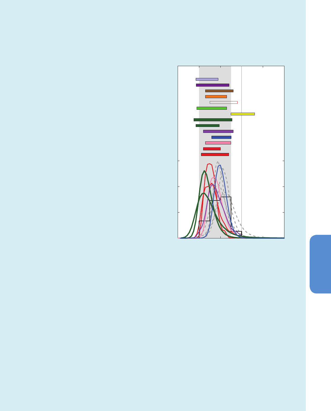
1111

Long-term Climate Change: Projections, Commitments and Irreversibility Chapter 12

Box 12.2 (continued)

formal statistical method to combine different lines of evidence. All methods in general are sensitive to the assumed prior distributions.

These limitations are discussed in detail in Section 10.8.2.

Based on the combined evidence from observed climate change including the observed 20th century warming, climate models, feed-

back analysis and paleoclimate, ECS is likely in the range 1.5°C to 4.5°C with high conﬁdence. The combined evidence increases

the conﬁdence in this ﬁnal assessment compared to that based

on the observed warming and paleoclimate only. ECS is posi-

tive, extremely unlikely less than 1°C (high conﬁdence), and very

unlikely greater than 6°C (medium conﬁdence). The upper limit of

the likely range is unchanged compared to AR4. The lower limit of

the likely range of 1.5°C is less than the lower limit of 2°C in AR4.

This change reﬂects the evidence from new studies of observed

temperature change, using the extended records in atmosphere

and ocean. These studies suggest a best ﬁt to the observed sur-

face and ocean warming for ECS values in the lower part of the

likely range. Note that these studies are not purely observation-

al, because they require an estimate of the response to RF from

models. In addition, the uncertainty in ocean heat uptake remains

substantial (see Section 3.2, Box 13.1). Accounting for short

term variability in simple models remains challenging, and it is

important not to give undue weight to any short time period that

might be strongly affected by internal variability (see Box 9.2).

On the other hand, AOGCMs show very good agreement with

observed climatology with ECS values in the upper part of the

1.5°C to 4.5°C range (Section 9.7.3.3), but the simulation of key

feedbacks like clouds remains challenging in those models. The

estimates from the observed warming, paleoclimate, and from

climate models are consistent within their uncertainties, each is

supported by many studies and multiple data sets, and in combi-

nation they provide high conﬁdence for the assessed likely range.

Even though this assessed range is similar to previous reports

(Charney, 1979; IPCC, 2001), conﬁdence today is much higher as

a result of high quality and longer observational records with a

clearer anthropogenic signal, better process understanding, more

and better understood evidence from paleoclimate reconstruc-

tions, and better climate models with higher resolution that cap-

ture many more processes more realistically. Box 12.2 Figure 1

illustrates that all these lines of evidence individually support the

assessed likely range of 1.5°C to 4.5°C.

The tails of the ECS distribution are now better understood. Multiple lines of evidence provide high conﬁdence that an ECS value less

than 1°C is extremely unlikely. The assessment that ECS is very unlikely greater than 6°C is an expert judgment informed by several

lines of evidence. First, the comprehensive climate models used in the CMIP5 exercise produce an ECS range of 2.1°C to 4.7°C (Table

9.5), very similar to CMIP3. Second, comparisons of perturbed-physics ensembles against the observed climate ﬁnd that models with

ECS values in the range 3°C to 4°C show the smallest errors for many ﬁelds (Section 9.7.3.3). Third, there is increasing evidence that the

aerosol RF of the 20th century is not strongly negative, which makes it unlikely that the observed warming was caused by a very large

ECS in response to a very small net forcing. Fourth, multiple and at least partly independent observational constraints from the satellite

period, instrumental period and palaeoclimate studies continue to yield very low probabilities for ECS larger than 6°C, particularly

when including most recent ocean and atmospheric data (see Box 12.2, Figure 1).

Analyses of observations and simulations of the instrumental period are estimating the effective climate sensitivity (a measure of the

strengths of the climate feedbacks today, see Glossary), rather than ECS directly. In some climate models ECS tends to be higher than

the effective climate sensitivity (see Section 12.5.3), because the feedbacks that are represented in the models (water vapour, lapse

Box 12.2, Figure 2 | Probability density functions, distributions and ranges

(5 to 95%) for the transient climate response from different studies, based on

Figure 10.20a, and results from CMIP5 (black histogram; Table 9.5). The grey

shaded range marks the likely 1°C to 2.5°C range, and the grey solid line marks

the extremely unlikely greater than 3°C. See Figure 10.20a and Chapter 10

Supplementary Material for full caption and details. Full references are given

in Section 10.8.

012 3 4 5

0.5

1.5

Knutti & Tomassini (2008) (b)

Knutti & Tomassini (2008) (a)

Black histogram

CMIP5 models

Dashed lines

AR4 studies

Meinshausen et al (2009)

Harris et al (2013)

Rogelj et al (2012)

Otto et al (2013) (a)

Otto et al (2013) (b)

Tung et al (2008)

Gillett et al (2013)

Stott & Forest (2007)

Gregory & Forster (2008)

Padilla et al (2011)

Libardoni & Forest (2011)

Schwartz (2012)

Transient Climate Response (°C)

Probability / Relative Frequency (°C

−1

)

(continued on next page)

1112

Chapter 12 Long-term Climate Change: Projections, Commitments and Irreversibility

12.5.4.3 Conclusions and Limitations

One difﬁculty with the concepts of climate stabilization and targets is

that stabilization of global temperature does not imply stabilization for

all aspects of the climate system. For example, some models show sig-

niﬁcant hysteresis behaviour in the global water cycle, because global

precipitation depends on both atmospheric CO

and temperature (Wu

et al., 2010). Processes related to vegetation changes (Jones et al.,

2009) or changes in the ice sheets (Charbit et al., 2008; Ridley et al.,

2010) as well as ocean acidiﬁcation, deep ocean warming and asso-

ciated sea level rise (Meehl et al., 2005b; Wigley, 2005; Zickfeld et al.,

2013) (see Figure 12.44d), and potential feedbacks linking, for exam-

ple, ocean and the ice sheets (Gillett et al., 2011; Goelzer et al., 2011),

have their own intrinsic long time scales. Those will result in signiﬁcant

changes hundreds to thousands of years after global temperature is

stabilized. Thermal expansion, in contrast to global mean temperature,

also depends on the evolution of surface temperature (Stouffer and

Manabe, 1999; Bouttes et al., 2013; Zickfeld et al., 2013).

Box 12.2 (continued)

rate, albedo and clouds) vary with the climate state. On time scales of many centuries, additional feedbacks with their own intrinsic

time scales (e.g., vegetation, ice sheets; see Sections 5.3.3 and 12.5.3) (Jones et al., 2009; Goelzer et al., 2011) may become important

but are not usually modelled. The resulting Earth system sensitivity is less well constrained but likely to be larger than ECS (Hansen et

al., 2008; Rohling et al., 2009; Lunt et al., 2010; Pagani et al., 2010; Rohling and Members, 2012), implying that lower atmospheric CO

concentrations are needed to meet a given temperature target on multi-century time scales. A number of caveats, however, apply to

those studies (see Section 12.5.3). Those long-term feedbacks have their own intrinsic time scales, and are less likely to be proportional

to global mean temperature change.

For scenarios of increasing RF, TCR is a more informative indicator of future climate than ECS (Frame et al., 2005; Held et al., 2010). This

assessment concludes with high conﬁdence that the TCR is likely in the range 1°C to 2.5°C, close to the estimated 5 to 95% range of

CMIP5 (1.2°C to 2.4°C; see Table 9.5), is positive and extremely unlikely greater than 3°C. As with the ECS, this is an expert-assessed

range, supported by several different and partly independent lines of evidence, each based on multiple studies, models and data sets.

TCR is estimated from the observed global changes in surface temperature, ocean heat uptake and RF, the detection/attribution studies

identifying the response patterns to increasing GHG concentrations (Section 10.8.1), and the results of CMIP3 and CMIP5 (Section

9.7.1). Estimating TCR suffers from fewer difﬁculties in terms of state- or time-dependent feedbacks (see Section 12.5.3), and is less

affected by uncertainty as to how much energy is taken up by the ocean. Unlike ECS, the ranges of TCR estimated from the observed

warming and from AOGCMs agree well, increasing our conﬁdence in the assessment of uncertainties in projections over the 21st

century.

Another useful metric relating directly CO

emissions to temperature is the transient climate response to cumulative carbon emission

(TCRE) (see Sections 12.5.4 and 10.8.4). This metric is useful to determine the allowed cumulative carbon emissions for stabilization at

a speciﬁc global temperature. TCRE is deﬁned as the annual mean global surface temperature change per unit of cumulated CO

emis-

sions, usually 1000 PgC, in a scenario with continuing emissions (see Glossary). It considers physical and carbon cycle feedbacks and

uncertainties, but not additional feedbacks associated for example with the release of methane hydrates or large amounts of carbon

from permafrost. The assessment based on climate models as well as the observed warming suggests that the TCRE is likely between

0.8°C to 2.5°C per 1000 PgC (10

metric tons of carbon), for cumulative CO

emissions less than about 2000 PgC until the time at which

temperatures peak. Under these conditions, and for low to medium estimates of climate sensitivity, the TCRE gives an accurate estimate

of the peak global mean temperature response to cumulated carbon emissions. TCRE has the advantage of directly relating global mean

surface temperature change to CO

emissions, but as a result of combining the uncertainty in both TCR and the carbon cycle response,

it is more uncertain. It also ignores non-CO

forcings and the fact that other components of the climate system (e.g., sea level rise, ice

sheets) have their own intrinsic time scales, resulting in climate change not avoided by limiting global temperature change.

The simplicity of the concept of a cumulative carbon emission budget

makes it attractive for policy (WBGU, 2009). The principal driver of long

term warming is the total cumulative emission of CO

over time. To

limit warming caused by CO

emissions to a given temperature target,

cumulative CO

emissions from all anthropogenic sources therefore

need to be limited to a certain budget. Higher emissions in earlier dec-

ades simply imply lower emissions by the same amount later on. This

is illustrated in the RCP2.6 scenario in Figure 12.46a/b. Two idealized

emission pathways with initially higher emissions (even sustained at

high level for a decade in one case) eventually lead to the same warm-

ing if emissions are then reduced much more rapidly. Even a stepwise

emission pathway with levels constant at 2010 and zero near mid-cen-

tury would eventually lead to a similar warming as they all have iden-

tical cumulative emissions.

However, several aspects related to the concept of a cumulative carbon

emission budget should be kept in mind. The ratio of global tempera-

ture and cumulative carbon is only approximately constant. It is the

result of an interplay of several compensating carbon cycle and climate

1113

Long-term Climate Change: Projections, Commitments and Irreversibility Chapter 12

feedback processes operating on different time scales (a cancellation of

variations in the increase in RF per ppm of CO

, the ocean heat uptake

efﬁciency and the airborne fraction) (Gregory et al., 2009; Matthews

et al., 2009; Solomon et al., 2009). It depends on the modelled climate

sensitivity and carbon cycle feedbacks. Thus, the allowed emissions for

a given temperature target are uncertain (see Figure 12.45) (Matthews

et al., 2009; Zickfeld et al., 2009; Knutti and Plattner, 2012). Neverthe-

less, the relationship is nearly linear in all models. Most models do not

consider the possibility that long term feedbacks (Hansen et al., 2007;

Knutti and Hegerl, 2008) may be different (see Section 12.5.3). Despite

the fact that stabilization refers to equilibrium, the results assessed

here are primarily relevant for the next few centuries and may differ

for millennial scales. Notably, many of these limitations apply similarly

to other policy targets, for example, stabilizing the atmospheric CO

concentration.

Non-CO

forcing constituents are important, which requires either

assumptions on how CO

emission reductions are linked to changes

in other forcings (Meinshausen et al., 2006; Meinshausen et al., 2009;

McCollum et al., 2013), or separate emission budgets and climate

modelling for short-lived and long-lived gases. So far, many studies

ignored non-CO

forcings altogether. Those that consider them ﬁnd

signiﬁcant effects, in particular warming of several tenths of a degree

for abrupt reductions in emissions of short-lived species, like aerosols

(Brasseur and Roeckner, 2005; Hare and Meinshausen, 2006; Zickfeld

et al., 2009; Armour and Roe, 2011; Tanaka and Raddatz, 2011) (see

also FAQ 12.3). Other studies, which model reductions that explicitly

target warming from short-lived non-CO

species only, ﬁnd important

short-term cooling beneﬁts shortly after the reduction of these species

(Shindell et al., 2012), but do not extend beyond 2030.

The concept of cumulative carbon also implies that higher initial emis-

sions can be compensated by a faster decline in emissions later or by

negative emissions. However, in the real world short-term and long-

term goals are not independent and mitigation rates are limited by

economic constraints and existing infrastructure (Rive et al., 2007;

Mignone et al., 2008; Meinshausen et al., 2009; Davis et al., 2010;

Friedlingstein et al., 2011; Rogelj et al., 2013). An analysis of 193

published emission pathways with an energy balance model (UNEP,

2010; Rogelj et al., 2011) is shown in Figure 12.46c, d. Those emission

pathways that likely limit warming below 2°C (above pre-industrial)

by 2100 show emissions of about 31 to 46 Pg(CO

-eq) yr

–1

and 17 to

23 Pg(CO

-eq) yr

–1

by 2020 and 2050, respectively. Median 2010 emis-

sions of all models are 48 Pg(CO

-eq) yr

–1

. Note that, as opposed to

Figure 12.46a, b, many scenarios still have positive emissions in 2100.

As these will not be zero immediately after 2100, they imply that the

warming may exceed the target after 2100.

The aspects discussed above do not limit the robustness of the overall

scientiﬁc assessment, but highlight factors that need to be considered

when determining cumulative CO

emissions consistent with a given

temperature target. In conclusion, taking into account the available

information from multiple lines of evidence (observations, models and

process understanding), the near linear relationship between cumula-

tive CO

emissions and peak global mean temperature is well estab-

lished in the literature and robust for cumulative total CO

emissions

up to about 2000 PgC. It is consistent with the relationship inferred

from past cumulative CO

emissions and observed warming, is sup-

ported by process understanding of the carbon cycle and global energy

balance, and emerges as a robust result from the entire hierarchy of

models.

Using a best estimate for the TCRE would provide a most likely value

for the cumulative CO

emissions compatible with stabilization at a

given temperature. However, such a budget would imply about 50%

probability for staying below the temperature target. Higher probabil-

ities for staying below a temperature or concentration target require

signiﬁcantly lower budgets (Knutti et al., 2005; Meinshausen et al.,

2009; Rogelj et al., 2012). Based on the assessment of TCRE (assum-

ing a normal distribution with a ±1 standard deviation range of 0.8-

2.5°C per 1000 PgC), limiting the warming caused by anthropogenic

emissions alone (i.e., ignoring other radiative forcings) to less than

2°C since the period 1861–1880 with a probability of >33%, >50%

and >66%, total CO

emissions from all anthropogenic sources would

need to be below a cumulative budget of about 1570 PgC, 1210 PgC

and 1000 PgC since 1870, respectively. An amount of 515 [445 to 585]

PgC was emitted between 1870 and 2011. Accounting for non-CO

forcings contributing to peak warming, or requiring a higher likelihood

of temperatures remaining below 2°C, both imply lower cumulative

emissions. A possible release of GHGs from permafrost or meth-

ane hydrates, not accounted for in current models, would also further

reduce the anthropogenic CO

emissions compatible with a given tem-

perature target. When accounting for the non-CO

forcings as in the

RCP scenarios, compatible carbon emissions since 1870 are reduced

to about 900 PgC, 820 PgC and 790 PgC to limit warming to less than

2°C since the period 1861–1880 with a probability of >33%, >50%,

and >66%, respectively. These estimates were derived by computing

the fraction of CMIP5 ESMs and EMICs that stay below 2°C for given

cumulative emissions following RCP8.5, as shown in TFE.8 Figure 1c.

The non-CO

forcing in RCP8.5 is higher than in RCP2.6. Because all

likelihood statements in calibrated IPCC language are open intervals,

the provided estimates are thus both conservative and consistent

choices valid for non-CO

forcings across all RCP scenarios. There is no

RCP scenario which limits warming to 2°C with probabilities of >33%

or >50%, and which could be used to directly infer compatible cumu-

lative emissions. For a probability of >66% RCP2.6 can be used as a

comparison. Combining the average back-calculated fossil fuel carbon

emissions for RCP2.6 between 2012 and 2100 (270 PgC) with the aver-

age historical estimate of 515 PgC gives a total of 785 PgC, i.e., 790

PgC when rounded to 10 PgC. As the 785 PgC estimate excludes an

explicit assessment of future land-use change emissions, the 790 PgC

value also remains a conservative estimate consistent with the overall

likelihood assessment. The ranges of emissions for these three likeli-

hoods based on the RCP scenarios are rather narrow, as they are based

on a single scenario and on the limited sample of models available

(TFE.8 Figure 1c). In contrast to TCRE they do not include observational

constraints or account for sources of uncertainty not sampled by the

models. The concept of a ﬁxed cumulative CO

budget holds not just for

2°C, but for any temperature level explored with models so far (up to

about 5°C; see Figures 12.44 to 12.46), with higher temperature levels

implying larger budgets.

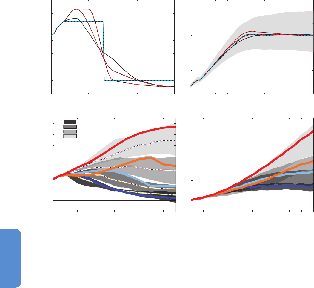
1114

Chapter 12 Long-term Climate Change: Projections, Commitments and Irreversibility

T<2°C

2°C<T<3°C

3°C<T<4°C

T>4°C

2000 2010 2020 2030 2040 2050 2060 2070 2080 2090 2100

Likely (>66%) temperature increase (T) during 21st century

from illustrative emission trajectories and RCPs

Total GHG emission levels (GtCO

-eq yr

-1

)

2000 2010 2020 2030 2040 2050 2060 2070 2080 2090 2100

Median temperature increase per pathway group (min-max)

and per RCP (median)

Temperature increase rel. to preindustrial (°C)

2000 2010 2020 2030 2040 2050 2060 2070 2080 2090 2100

-2

Year

emissions from fossil fuel and industry (GtC yr

-1

)

2000 2010 2020 2030 2040 2050 2060 2070 2080 2090 2100

0.8

1.2

1.4

1.6

1.8

2.2

Year

Year Year

Temperature increase relative to preindustrial (°C)

-20

100

120

140

12.5.5 Potentially Abrupt or Irreversible Changes

12.5.5.1 Introduction

This report adopts the deﬁnition of abrupt climate change used in Syn-

thesis and Assessment Product 3.4 of the U.S. Climate Change Science

Program CCSP (CCSP, 2008b). We deﬁne abrupt climate change as a

large-scale change in the climate system that takes place over a few

decades or less, persists (or is anticipated to persist) for at least a few

decades, and causes substantial disruptions in human and natural sys-

tems (see Glossary). Other deﬁnitions of abrupt climate change exist.

For example, in the AR4 climate change was deﬁned as abrupt if it

occurred faster than the typical time scale of the responsible forcing.

A number of components or phenomena within the Earth system have

been proposed as potentially possessing critical thresholds (some-

Figure 12.46 | (a) CO

emissions for the RCP2.6 scenario (black) and three illustrative modiﬁed emission pathways leading to the same warming. (b) Global temperature change

relative to pre-industrial for the pathways shown in panel (a). (c) Grey shaded bands show Integrated Assessment Model (IAM) emission pathways over the 21st century. The

pathways were grouped based on ranges of likely avoided temperature increase in the 21st century. Pathways in the darkest three bands likely stay below 2°C, 3°C, 4°C by 2100,

respectively (see legend), while those in the lightest grey band are higher than that. Emission corridors were deﬁned by, at each year, identifying the 15th to 85th percentile range of

emissions and drawing the corresponding bands across the range. Individual scenarios that follow the upper edge of the bands early on tend to follow the lower edge of the band

later on. Black-white lines show median paths per range. (d) Global temperature relative to pre-industrial for the pathways in (c). (Data in (c) and (d) based on Rogelj et al. (2011).)

Coloured lines in (c) and (d) denote the four RCP scenarios.

times referred to as tipping points (Lenton et al., 2008)), beyond which

abrupt or nonlinear transitions to a different state ensues. The term

irreversibility is used in various ways in the literature. The AR5 report

deﬁnes a perturbed state as irreversible on a given time scale if the

recovery time scale from this state due to natural processes is sig-

niﬁcantly longer than the time it takes for the system to reach this

perturbed state (see Glossary). In that context, most aspects of the cli-

mate change resulting from CO

emissions are irreversible, due to the

long residence time of the CO

perturbation in the atmosphere and the

resulting warming (Solomon et al., 2009). These results are discussed

in Sections 12.5.2 to 12.5.4. Here, we also assess aspects of irreversi-

bility in the context of abrupt change, multiple steady states and hys-

teresis, i.e., the question whether a change (abrupt or not) would be

reversible if the forcing was reversed or removed (e.g., Boucher et al.,

2012). Irreversibility of ice sheets and sea level rise are also assessed

in Chapter 13.

1115

Long-term Climate Change: Projections, Commitments and Irreversibility Chapter 12

In this section we examine the main components or phenomena within

the Earth system that have been proposed in the literature as potential-

ly being susceptible to abrupt or irreversible change (see Table 12.4).

Abrupt changes that arise from nonlinearities within the climate system

are inherently difﬁcult to assess and their timing, if any, of future occur-

rences is difﬁcult to predict. Nevertheless, progress is being made

exploring the potential existence of early warning signs for abrupt cli-

mate change (see e.g., Dakos et al., 2008; Scheffer et al., 2009).

12.5.5.2 The Atlantic Meridional Overturning

EMICs for which the stability has been systematically assessed by

suitably designed hysteresis experiments robustly show a threshold

beyond which the Atlantic thermohaline circulation cannot be sus-

tained (Rahmstorf et al., 2005). This is also the case for one low-reso-

lution ESM (Hawkins et al., 2011). However, proximity to this threshold

is highly model dependent and inﬂuenced by factors that are currently

poorly understood. There is some indication that the CMIP3 climate

models may generally overestimate the stability of the Atlantic Ocean

circulation (Hofmann and Rahmstorf, 2009; Drijfhout et al., 2010). In

particular, De Vries and Weber (2005), Dijkstra (2007), Weber et al.

(2007), Huisman et al. (2010), Drijfhout et al. (2010) and Hawkins et

al. (2011) suggest that the sign of net freshwater ﬂux into the Atlantic

transported through its southern boundary via the overturning circu-

lation determines whether or not the AMOC is in a mono-stable or

bi-stable state. For the pre-industrial control climate of most of the

CMIP3 models, Drijfhout et al. (2010) found that the salt ﬂux was nega-

tive (implying a positive freshwater ﬂux), indicating that they were in a

mono-stable regime. However, this is not the case in the CMIP5 models

where Weaver et al. (2012) found that the majority of the models were

in a bi-stable regime during RCP integrations. Observations suggest

that the present day ocean is in a bi-stable regime, thereby allowing

for multiple equilibria and a stable ‘off’ state of the AMOC (Bryden et

al., 2011; Hawkins et al., 2011).

Change in climate

system component

Potentially

abrupt (AR5

deﬁnition)

Irreversibility if

forcing reversed

Projected likelihood of 21st century change in scenarios considered

Atlantic MOC collapse Yes Unknown Very unlikely that the AMOC will undergo a rapid transition (high conﬁdence)

Ice sheet collapse No Irreversible for millennia Exceptionally unlikely that either Greenland or West Antarctic Ice sheets

will suffer near-complete disintegration (high conﬁdence)

Permafrost carbon release No Irreversible for millennia Possible that permafrost will become a net source of atmospheric greenhouse gases (low conﬁdence)

Clathrate methane release Yes Irreversible for millennia Very unlikely that methane from clathrates will undergo catastrophic release (high conﬁdence)

Tropical forests dieback Yes Reversible within

centuries

Low conﬁdence in projections of the collapse of large areas of tropical forest

Boreal forests dieback Yes Reversible within

centuries

Low conﬁdence in projections of the collapse of large areas of boreal forest

Disappearance of

summer Arctic sea ice

Yes Reversible within

years to decades

Likely that the Arctic Ocean becomes nearly ice-free in September before mid-cen-

tury under high forcing scenarios such as RCP8.5 (medium conﬁdence)

Long-term droughts Yes Reversible within

years to decades

Low conﬁdence in projections of changes in the frequency and duration of megadroughts

Monsoonal circulation Yes Reversible within

years to decades

Low conﬁdence in projections of a collapse in monsoon circulations

Table 12.4 | Components in the Earth system that have been proposed in the literature as potentially being susceptible to abrupt or irreversible change. Column 2 deﬁnes whether

or not a potential change can be considered to be abrupt under the AR5 deﬁnition. Column 3 states whether or not the process is irreversible in the context of abrupt change, and

also gives the typical recovery time scales. Column 4 provides an assessment, if possible, of the likelihood of occurrence of abrupt change in the 21st century for the respective

components or phenomena within the Earth system, for the scenarios considered in this chapter.

In addition to the main threshold for a complete breakdown of the

circulation, others may exist that involve more limited changes, such as

a cessation of Labrador Sea deep water formation (Wood et al., 1999).

Rapid melting of the Greenland ice sheet causes increases in freshwa-

ter runoff, potentially weakening the AMOC. None of the CMIP5 sim-

ulations include an interactive ice sheet component. However, Jung-

claus et al. (2006), Mikolajewicz et al. (2007), Driesschaert et al. (2007)

and Hu et al. (2009) found only a slight temporary effect of increased

melt water ﬂuxes on the AMOC, that was either small compared to the

effect of enhanced poleward atmospheric moisture transport or only

noticeable in the most extreme scenarios.

Although many more model simulations have been conducted since

the AR4 under a wide range of forcing scenarios, projections of the

AMOC behaviour have not changed. Based on the available CMIP5

models, EMICs and the literature, it remains very likely that the AMOC

will weaken over the 21st century relative to pre-industrial. Best esti-

mates and ranges for the reduction from CMIP5 are 11% (1 to 24%)

in RCP2.6 and 34% (12 to 54%) in RCP8.5 (Weaver et al., 2012) (see

Section 12.4.7.2, Figure 12.35). But there is low conﬁdence in the mag-

nitude of the weakening. Drijfhout et al. (2012) show that the AMOC

decrease per degree global mean temperature rise varies from 1.5 to

1.9 Sv (10

–1

) for the CMIP5 multi-model ensemble members they

considered depending on the scenario, but that the standard deviation

in this regression is almost half the signal.

The FIO-ESM model shows cooling over much of the NH that may be

related to a strong reduction of the AMOC in all RCP scenarios (even

RCP2.6), but the limited output available from the model precludes

an assessment of the response and realism of this response. Hence

it is not included the overall assessment of the likelihood of abrupt

changes.

1116

Chapter 12 Long-term Climate Change: Projections, Commitments and Irreversibility

It is unlikely that the AMOC will collapse beyond the end of the 21st

century for the scenarios considered but a collapse beyond the 21st

century for large sustained warming cannot be excluded.There is low

conﬁdence in assessing the evolution of the AMOC beyond the 21st

century. Two of the CMIP5 models revealed an eventual slowdown of

the AMOC to an off state (Figure 12.35). But this did not occur abruptly.

As assessed by Delworth et al. (2008), for an abrupt transition of the

AMOC to occur, the sensitivity of the AMOC to forcing would have

to be far greater that seen in current models. Alternatively, signiﬁcant

ablation of the Greenland ice sheet greatly exceeding even the most

aggressive of current projections would be required (Swingedouw et

al., 2007; Hu et al., 2009). While neither possibility can be excluded

entirely, it is unlikely that the AMOC will collapse beyond the end of

the 21st century because of global warming based on the models and

range of scenarios considered.

12.5.5.3 Ice Sheets

As detailed in Section 13.4.3, all available modelling studies agree that

the Greenland ice sheet will signiﬁcantly decrease in area and volume

in a warmer climate as a consequence of increased melt rates not

compensated for by increased snowfall rates and ampliﬁed by positive

feedbacks. Conversely, the surface mass balance of the Antarctic ice

sheet is projected to increase in most projections because increased

snowfall rates outweigh melt increase (see Section 13.4.4).

Irreversibility of ice sheet volume and extent changes can arise because

of the surface-elevation feedback that operates when a decrease of the

elevation of the ice sheet induces a decreased surface mass balance

(generally through increased melting), and therefore essentially applies

to Greenland. As detailed in Section 13.4.3.3, several stable states of

the Greenland ice sheet might exist (Charbit et al., 2008; Ridley et al.,

2010; Langen et al., 2012; Robinson et al., 2012; Solgaard and Langen,

2012), and the ice sheet might irreversibly shrink to a stable small-

er state once a warming threshold is crossed for a certain amount of

time, with the critical duration depending on how far the temperature

threshold has been exceeded. Based on the available evidence (see

Section 13.4.3.3), an irreversible decrease of the Greenland ice sheet

due to surface mass balance changes appears very unlikely in the 21st

century but likely on multi-centennial to millennial time scales in the

strongest forcing scenarios.

In theory (Weertman, 1974; Schoof, 2007) ice sheet volume and extent

changes can be abrupt because of the grounding line instability that

can occur in coastal regions where bedrock is retrograde (i.e., sloping

towards the interior of the ice sheet) and below sea level (see Sec-

tion 4.4.4 and Box 13.2). This essentially applies to West Antarctica,

but also to parts of Greenland and East Antarctica. Furthermore, ice

shelf decay induced by oceanic or atmospheric warming might lead to

abruptly accelerated ice ﬂow further inland (De Angelis and Skvarca,

2003). Because ice sheet growth is usually a slow process, such chang-

es could also be irreversible in the deﬁnition adopted here. The availa-

ble evidence (see Section 13.4) suggests that it is exceptionally unlikely

that the ice sheets of either Greenland or West Antarctica will suffer a

near-complete disintegration during the 21st century. More generally,

the potential for abrupt and/or irreversible ice sheet changes (or the

initiation thereof) during the 21st century and beyond is discussed in

detail in Sections 13.4.3 and 13.4.4.

12.5.5.4 Permafrost Carbon Storage

Since the IPCC AR4, estimates of the amount of carbon stored in

permafrost have been signiﬁcantly revised upwards (Tarnocai et al.,

2009), putting the permafrost carbon stock to an equivalent of twice

the atmospheric carbon pool (Dolman et al., 2010). Because of low

carbon input at high latitudes, permafrost carbon is to a large part of

Pleistocene (Zimov et al., 2006) or Holocene (Smith et al., 2004) origin,

and its potential vulnerability is dominated by decomposition (Eglin et

al., 2010). The conjunction of a long carbon accumulation time scale on

one hand and potentially rapid permafrost thawing and carbon decom-

position under warmer climatic conditions (Zimov et al., 2006; Schuur

et al., 2009; Kuhry et al., 2010) on the other hand suggests poten-

tial irreversibility of permafrost carbon decomposition (leading to an

increase of atmospheric CO

and/or CH

concentrations) on time scales

of hundreds to thousands of years in a warming climate. Indeed, recent

observations (Dorrepaal et al., 2009; Kuhry et al., 2010) suggest that

this process, induced by widespread permafrost warming and thaw-

ing (Romanovsky et al., 2010), might be already occurring. However,

the existing modelling studies of permafrost carbon balance under

future warming that take into account at least some of the essen-

tial permafrost-related processes (Khvorostyanov et al., 2008; Wania

et al., 2009; Koven et al., 2011; Schaefer et al., 2011; MacDougall et

al., 2012; Schneider von Deimling et al., 2012) do not yield coherent

results beyond the fact that present-day permafrost might become a

net emitter of carbon during the 21st century under plausible future

warming scenarios (low conﬁdence). This also reﬂects an insufﬁcient

understanding of the relevant soil processes during and after perma-

frost thaw, including processes leading to stabilization of unfrozen soil

carbon (Schmidt et al., 2011), and precludes a ﬁrm assessment of the

amplitude of irreversible changes in the climate system potentially

related to permafrost degassing and associated global feedbacks at

this stage (see also Sections 6.4.3.4 and 6.4.7.2 and FAQ 6.1).

12.5.5.5 Atmospheric Methane from Terrestrial and Oceanic

Clathrates

Model simulations (Fyke and Weaver, 2006; Reagan and Moridis, 2007;

Lamarque, 2008; Reagan and Moridis, 2009) suggest that clathrate

deposits in shallow regions (in particular at high latitude regions and in

the Gulf of Mexico) are susceptible to destabilization via ocean warm-

ing. However, concomitant sea level rise due to changes in ocean mass

enhances clathrate stability in the ocean (Fyke and Weaver, 2006). A

recent assessment of the potential for a future abrupt release of meth-

ane was undertaken by the U.S. Climate Change Science Program (Syn-

thesis and Assessment Product 3.4 see Brooke et al., 2008). They con-

cluded that it was very unlikely that such a catastrophic release would

occur this century. However, they argued that anthropogenic warming

will very likely lead to enhanced methane emissions from both terres-

trial and oceanic clathrates (Brooke et al., 2008). Although difﬁcult to

formally assess, initial estimates of the 21st century positive feedback

from methane clathrate destabilization are small but not insigniﬁcant

(Fyke and Weaver, 2006; Archer, 2007; Lamarque, 2008). Nevertheless,

on multi-millennial time scales, the positive feedback to anthropogenic

1117

Long-term Climate Change: Projections, Commitments and Irreversibility Chapter 12

warming of such methane emissions is potentially larger (Archer and

Buffett, 2005; Archer, 2007; Brooke et al., 2008). Once more, due to the

difference between release and accumulation time scales, such emis-

sions are irreversible. See also FAQ 6.1.

12.5.5.6 Tropical and Boreal Forests

12.5.5.6.1 Tropical forests

In today’s climate, the strongest growth in the Amazon rainforest

occurs during the dry season when strong insolation is combined with

water drawn from underground aquifers that store the previous wet

season’s rainfall (Huete et al., 2006). AOGCMs do not agree about how

the dry season length in the Amazon may change in the future under

the SRES A1 scenario (Bombardi and Carvalho, 2009), but simulations

with coupled regional climate/potential vegetation models are consist-

ent in simulating an increase in dry season length, a 70% reduction in

the areal extent of the rainforest by the end of the 21st century using

the SRES A2 scenario, and an eastward expansion of the Caatinga

vegetation (Cook and Vizy, 2008; Sorensson et al., 2010). In addition,

some models have demonstrated the existence of multiple equilibria of

the tropical South American climate–vegetation system (e.g., Oyama

and Nobre, 2003). The transition could be abrupt when the dry season

becomes too long for the vegetation to survive, although the resilience

of the vegetation to a longer dry period may be increased by the CO

fertilization effect (Zelazowski et al., 2011). Deforestation may also

increase dry season length (Costa and Pires, 2010) and drier conditions

increase the likelihood of wildﬁres that, combined with ﬁre ignition

associated with human activity, can undermine the forest’s resiliency

to climate change (see also Section 6.4.8.1). If climate change brings

drier conditions closer to those supportive of seasonal forests rather

than rainforest, ﬁre can act as a trigger to abruptly and irreversibly

change the ecosystem (Malhi et al., 2009). However, the existence of

refugia is an important determinant of the potential for the re-emer-

gence of the vegetation (Walker et al., 2009).

Analysis of projected change in the climate–biome space of current

vegetation distributions suggest that the risk of Amazonian forest die-

back is small (Malhi et al., 2009), a ﬁnding supported by modelling

when strong carbon dioxide fertilization effects on Amazonian vegeta-

tion are assumed (Rammig et al., 2010). However, the strength of CO

fertilization on tropical vegetation is poorly known (see Box 6.3). Uncer-

tainty concerning the existence of critical thresholds in the Amazonian

and other tropical rainforests purely driven by climate change therefore

remains high, and so the possibility of a critical threshold being crossed

in precipitation volume cannot be ruled out (Nobre and Borma, 2009;

Good et al., 2011b, 2011c). Nevertheless, there is still some question as

to whether a transition of the Amazonian or other tropical rainforests

into a lower biomass state could result from the combined effects of

limits to carbon fertilization, climate warming, potential precipitation

decline in interaction with the effects of human land use.

12.5.5.6.2 Boreal forest

Evidence from ﬁeld observations and biogeochemical modelling make it

scientiﬁcally conceivable that regions of the boreal forest could tip into

a different vegetation state under climate warming, but uncertainties

on the likelihood of this occurring are very high (Lenton et al., 2008;

Allen et al., 2010). This is mainly due to large gaps in knowledge con-

cerning relevant ecosystemic and plant physiological responses to

warming (Niinemets, 2010). The main response is a potential advance-

ment of the boreal forest northward and the potential transition from

a forest to a woodland or grassland state on its dry southern edges in

the continental interiors, leading to an overall increase in herbaceous

vegetation cover in the affected parts of the boreal zone (Lucht et al.,

2006). The proposed potential mechanisms for decreased forest growth

and/or increased forest mortality are: increased drought stress under

warmer summer conditions in regions with low soil moisture (Barber et

al., 2000; Dulamsuren et al., 2009, 2010); desiccation of saplings with

shallow roots due to summer drought periods in the top soil layers,

causing suppression of forest reproduction (Hogg and Schwarz, 1997);

leaf tissue damage due to high leaf temperatures during peak summer

temperatures under strong climate warming; and increased insect, her-

bivory and subsequent ﬁre damage in damaged or struggling stands

(Dulamsuren et al., 2008). The balance of effects controlling standing

biomass, ﬁre type and frequency, permafrost thaw depth, snow volume

and soil moisture remains uncertain. Although the existence of, and the

thresholds controlling, a potential critical threshold in the boreal forest

are extremely uncertain, its existence cannot at present be ruled out.

12.5.5.7 Sea Ice

Several studies based on observational data or model hindcasts sug-

gest that the rapidly declining summer Arctic sea ice cover might reach

or might already have passed a tipping point (Lindsay and Zhang, 2005;

Wadhams, 2012; Livina and Lenton, 2013). Identifying Arctic sea ice tip-

ping points from the short observational record is difﬁcult due to high

interannual and decadal variability. In some climate projections, the

decrease in summer Arctic sea ice areal coverage is not gradual but is

instead punctuated by 5- to10- year periods of strong ice loss (Holland

et al., 2006; Vavrus et al., 2012; Döscher and Koenigk, 2013). Still, these

abrupt reductions do not necessarily require the existence of a tipping

point in the system or further imply an irreversible behaviour (Amstrup

et al., 2010; Lenton, 2012). The 5- to 10-year events discussed by Hol-

land et al. (2006) arise when large natural climate variability in the

Arctic reinforces the anthropogenically-forced change (Holland et al.,

2008). Positive trends on the same time scale also occur when internal

variability counteracts the forced change until the middle of the 21st

century (Holland et al., 2008; Kay et al., 2011; Vavrus et al., 2012).

Further work using single-column energy-balance models (Merryﬁeld

et al., 2008; Eisenman and Wettlaufer, 2009; Abbot et al., 2011) yielded

mixed results about the possibility of tipping points and bifurcations

in the transition from perennial to seasonal sea ice cover. Thin ice and

snow covers promote strong longwave radiative loss to space and high

ice growth rates (e.g., Bitz and Roe, 2004; Notz, 2009; Eisenman, 2012).

These stabilizing negative feedbacks can be large enough to overcome

the positive surface–albedo feedback and/or cloud feedback, which act

to amplify the forced sea ice response. In such low-order models, the

emergence of multiple stable states with increased climate forcing is a

parameter-dependent feature (Abbot et al., 2011; Eisenman, 2012). For

example, Eisenman (2012) showed with a single-column energy-bal-

ance model that certain parameter choices that cause thicker ice or

warmer ocean under a given climate forcing make the model more

prone to bifurcations and hence irreversible behaviour.

1118

Chapter 12 Long-term Climate Change: Projections, Commitments and Irreversibility

The reversibility of sea ice loss with respect to global or hemispher-

ic mean surface temperature change has been directly assessed in

AOGCMs/ESMs by ﬁrst raising the CO

concentration until virtually all

sea ice disappears year-round and then lowering the CO

level at the

same rate as during the ramp-up phase until it reaches again the initial

value (Armour et al., 2011; Boucher et al., 2012; Ridley et al., 2012; Li et

al., 2013b). None of these studies show evidence of a bifurcation lead-

ing to irreversible changes in Arctic sea ice. AOGCMs have also been

used to test summer Arctic sea ice recovery after either sudden or very

rapid artiﬁcial removal, and all had sea ice return within a few years

(Schröder and Connolley, 2007; Sedláček et al., 2011; Tietsche et al.,

2011). In the Antarctic, as a result of the strong coupling between the

Southern Ocean’s surface and the deep ocean, the sea ice areal cover-

age in some of the models integrated with ramp-up and ramp-down

atmospheric CO

concentration exhibits a signiﬁcant lag relative to the

global or hemispheric mean surface temperature (Ridley et al., 2012;

Li et al., 2013b), so that its changes may be considered irreversible on

centennial time scales.

Diagnostic analyses of a few global climate models have shown abrupt

sea ice losses in the transition from seasonal to year-round Arctic ice-

free conditions after raising CO

to very high levels (Winton, 2006b;

Ridley et al., 2008; Li et al., 2013b), but without evidence for irreversi-

ble changes. Winton (2006b, 2008) hypothesized that the small ice cap

instability (North, 1984) could cause such an abrupt transition. With a

low-order Arctic sea ice model, Eisenman and Wettlaufer (2009) also

found an abrupt change behaviour in the transition from seasonal ice

to year-round ice-free conditions, accompanied by an irreversible bifur-

cation to a new stable, annually ice-free state. They concluded that the

cause is a loss of the stabilizing effect of sea ice growth when the ice

season shrinks in time. The Arctic sea ice may thus experience a sharp

transition to annually ice-free conditions, but the irreversible nature of

this transition seems to depend on the model complexity and structure.

In conclusion, rapid summer Arctic sea ice losses are likely to occur in

the transition to seasonally ice-free conditions. These abrupt changes

might have consequences throughout the climate system as noted by

Vavrus et al. (2011) for cloud cover and Lawrence et al. (2008b) for the

high-latitude ground state. Furthermore, the interannual-to-decadal

variability in the summer Arctic sea ice extent is projected to increase in

response to global warming (Holland et al., 2008; Goosse et al., 2009).

These studies suggest that large anomalies in Arctic sea ice areal cov-

erage, like the ones that occurred in 2007 and 2012, might become

increasingly frequent. However, there is little evidence in global climate

models of a tipping point (or critical threshold) in the transition from

a perennially ice-covered to a seasonally ice-free Arctic Ocean beyond

which further sea ice loss is unstoppable and irreversible.

12.5.5.8 Hydrologic Variability: Long-Term Droughts and

Monsoonal Circulation

12.5.5.8.1 Long-term Droughts

As noted in Section 5.5.5, long-term droughts (often called mega-

droughts, see Glossary) are a recurring feature of Holocene paleocli-

mate records in North America, East and South Asia, Europe, Africa and

India. The transitions into and out of the long-term droughts take many

years. Because the long-term droughts all ended, they are not irrevers-

ible. Nonetheless transitions over years to a decade into a state of

long-term drought would have impacts on human and natural systems.

AR4 climate model projections (Milly et al., 2008) and CMIP5 ensem-

bles (Figure 12.23) both suggest widespread drying and drought across

most of southwestern North America and many other subtropical

regions by the mid to late 21st century (see Section 12.4.5), although

without abrupt change. Some studies suggest that this subtropical

drying may have already begun in southwestern North America (Seager

et al., 2007; Seidel and Randel, 2007; Barnett et al., 2008; Pierce et al.,

2008). More recent studies (Hoerling et al., 2010; Seager and Vecchi,

2010; Dai, 2011; Seager and Naik, 2012) suggest that regional reduc-

tions in precipitation are due primarily to internal variability and that

the anthropogenic forced trends are currently weak in comparison.

While previous long-term droughts in southwest North America arose

from natural causes, climate models project that this region will under-

go progressive aridiﬁcation as part of a general drying and poleward

expansion of the subtropical dry zones driven by rising GHGs (Held and

Soden, 2006; Seager et al., 2007; Seager and Vecchi, 2010). The models

project the aridiﬁcation to intensify steadily as RF and global warm-

ing progress without abrupt changes. Because of the very long life-

time of the anthropogenic atmospheric CO

perturbation, such drying

induced by global warming would be largely irreversible on millennium

time scale (Solomon et al., 2009; Frölicher and Joos, 2010; Gillett et

al., 2011) (see Sections 12.5.2 and 12.5.4). For example, Solomon et

al. (2009) found in a simulation where atmospheric CO

increases to

600 ppm followed by zero emissions, that the 15% reduction in pre-

cipitation in areas such as southwest North America, southern Europe

and western Australia would persist long after emissions ceased. This,

however, is largely a consequence of the warming persisting for centu-

ries after emissions cease rather than an irreversible behaviour of the

water cycle itself.

12.5.5.8.2 Monsoonal circulation

Climate model simulations and paleo-reconstructions provide evidence

of past abrupt changes in Saharan vegetation, with the ‘green Sahara’

conditions (Hoelzmann et al., 1998) of the African Humid Period (AHP)

during the mid-Holocene serving as the most recent example. However,

Mitchell (1990) and Claussen et al. (2003) note that the mid-Holocene is

not a direct analogue for future GHG-induced climate change since the

forcings are different: a increased shortwave forcing in the NH summer

versus a globally and seasonally uniform atmospheric CO

increase,

respectively. Paleoclimate examples suggest that a strong radiative

or SST forcing is needed to achieve a rapid climate change, and that

the rapid changes are reversible when the forcing is withdrawn. Both

the abrupt onset and termination of the AHP were triggered when

northern African summer insolation was 4.2% higher than present

day, representing a local increase of about 19 W m

–2

(deMenocal et

al., 2000). Note that the globally averaged radiative anthropogenic

forcing from 1750 to 2011 (Table 8.6) is small compared to this local

increase in insolation. A rapid Saharan greening has been simulated in

a climate model of intermediate complexity forced by a rapid increase

in atmospheric CO

, with the overall extent of greening depending on

the equilibrium atmospheric CO

level reached (Claussen et al., 2003).

1119

Long-term Climate Change: Projections, Commitments and Irreversibility Chapter 12

Abrupt Saharan vegetation changes of the Younger Dryas are linked

with a rapid AMOC weakening which is considered very unlikely during

the 21st century and unlikely beyond that as a consequence of global

warming.

Studies with conceptual models (Zickfeld et al., 2005; Levermann et

al., 2009) have shown that the Indian summer monsoon can operate

in two stable regimes: besides the ‘wet’ summer monsoon, a stable

state exists which is characterized by low precipitation over India.

These studies suggest that any perturbation of the radiative budget

that tends to weaken the driving pressure gradient has the potential to

induce abrupt transitions between these two regimes.

Numerous studies with coupled ocean–atmosphere models have

explored the potential impact of anthropogenic forcing on the Indian

monsoon (see also Section 14.2). When forced with anticipated increas-

es in GHG concentrations, the majority of these studies show an inten-

siﬁcation of the rainfall associated with the Indian summer monsoon

(Meehl and Washington, 1993; Kitoh et al., 1997; Douville et al., 2000;

Hu et al., 2000; May, 2002; Ueda et al., 2006; Kripalani et al., 2007; Sto-

wasser et al., 2009; Cherchi et al., 2010). Despite the intensiﬁcation of

precipitation, several of these modelling studies show a weakening of

the summer monsoon circulation (Kitoh et al., 1997; May, 2002; Ueda

et al., 2006; Kripalani et al., 2007; Stowasser et al., 2009; Cherchi et al.,

2010). The net effect is nevertheless an increase of precipitation due to

enhanced moisture transport into the Asian monsoon region (Ueda et

al., 2006). In recent years, studies with GCMs have also explored the

direct effect of aerosol forcing on the Indian monsoon (Lau et al., 2006;

Meehl et al., 2008; Randles and Ramaswamy, 2008; Collier and Zhang,

2009). Considering absorbing aerosols (black carbon) only, Meehl et

al. (2008) found an increase in pre-monsoonal precipitation, but a

decrease in summer monsoon precipitation over parts of South Asia. In

contrast, Lau et al. (2006) found an increase in May–June–July precipi-

tation in that region. If an increase in scattering aerosols only is consid-

ered, the monsoon circulation weakens and precipitation is inhibited

(Randles and Ramaswamy, 2008). More recently, Bollasina et al. (2011)

showed that anthropogenic aerosols played a fundamental role in driv-

ing the recent observed weakening of the summer monsoon. Given

that the effect of increased atmospheric regional loading of aerosols

is opposed by the concomitant increases in GHG concentrations, it is

unlikely that an abrupt transition to the dry summer monsoon regime

will be triggered in the 21st century.

Acknowledgements

We especially acknowledge the input of Contributing Authors Urs

Beyerle for maintaining the database of CMIP5 output, Jan Sedláček

for producing a large number of CMIP5 ﬁgures, and Joeri Rogelj for

preparing synthesis ﬁgures. Chapter technical assistants Oliver Stebler,

Franziska Gerber and Barbara Aellig, provided great help in assembling

the chapter and Sébastien Denvil and Jérôme Raciazek provided tech-

nical assistance in downloading the CMIP5 data.

1120

Chapter 12 Long-term Climate Change: Projections, Commitments and Irreversibility

References

Abbot, D. S., M. Silber, and R. T. Pierrehumbert, 2011: Bifurcations leading to summer

Arctic sea ice loss. J. Geophys. Res., 116, D19120.

Abe, M., H. Shiogama, T. Nozawa, and S. Emori, 2011: Estimation of future surface

temperature changes constrained using the future-present correlated modes in

inter-model variability of CMIP3 multimodel simulations. J. Geophys. Res., 116,

D18104.

Adachi, Y., et al., 2013: Basic performance of a new earth system model of the

Meteorological Research Institute (MRI-ESM1). Papers Meteorol. Geophys.,

doi:10.2467/mripapers.64.

Adams, P. J., J. H. Seinfeld, D. Koch, L. Mickley, and D. Jacob, 2001: General circulation

model assessment of direct radiative forcing by the sulfate-nitrate-ammonium-

water inorganic aerosol system. J. Geophys. Res., 106, 1097–1111.

Adler, R. F., G. J. Gu, J. J. Wang, G. J. Huffman, S. Curtis, and D. Bolvin, 2008:

Relationships between global precipitation and surface temperature on

interannual and longer timescales (1979–2006). J. Geophys. Res., 113, D22104.

Aldrin, M., M. Holden, P. Guttorp, R. B. Skeie, G. Myhre, and T. K. Berntsen, 2012:

Bayesian estimation of climate sensitivity based on a simple climate model

ﬁtted to observations of hemispheric temperatures and global ocean heat

content. Environmetrics, 23, 253–271.

Alexander, L. V., and J. M. Arblaster, 2009: Assessing trends in observed and modelled

climate extremes over Australia in relation to future projections. Int. J. Climatol.,

29, 417–435.

Alexander, L. V., et al., 2006: Global observed changes in daily climate extremes of

temperature and precipitation. J. Geophys. Res., 111, D05109.

Alexeev, V., and C. Jackson, 2012: Polar ampliﬁcation: Is atmospheric heat transport

important? Clim. Dyn., doi:10.1007/s00382-012-1601-z.

Alexeev, V., D. Nicolsky, V. Romanovsky, and D. Lawrence, 2007: An evaluation of

deep soil conﬁgurations in the CLM3 for improved representation of permafrost.

Geophys. Res. Lett., 34, L09502.

Alexeev, V. A., P. L. Langen, and J. R. Bates, 2005: Polar ampliﬁcation of surface

warming on an aquaplanet in “ghost forcing” experiments without sea ice

feedbacks. Clim. Dyn., 24, 655–666.

Allan, R., and B. Soden, 2008: Atmospheric warming and the ampliﬁcation of

precipitation extremes. Science, 321, 1481–1484.

Allan, R. P., 2012: Regime dependent changes in global precipitation. Clim. Dyn.,

doi:10.1007/s00382-011-1134-x.

Allen, C., et al., 2010: A global overview of drought and heat-induced tree mortality

reveals emerging climate change risks for forests. Forest Ecol. Manage., 259,

660–684.

Allen, M. R., and W. J. Ingram, 2002: Constraints on future changes in climate and

the hydrologic cycle. Nature, 419, 224–232.

Allen, M. R., D. J. Frame, C. Huntingford, C. D. Jones, J. A. Lowe, M. Meinshausen,

and N. Meinshausen, 2009: Warming caused by cumulative carbon emissions

towards the trillionth tonne. Nature, 458, 1163–1166.

Allen, R. J., and S. C. Sherwood, 2008: Warming maximum in the tropical upper

troposphere deduced from thermal winds. Nature Geosci., 1, 399–403.

Allen, R. J., and S. C. Sherwood, 2010: Aerosol-cloud semi-direct effect and land-sea

temperature contrast in a GCM. Geophys. Res. Lett., 37, L07702.

Allen, R. J., S. C. Sherwood, J. R. Norris, and C. S. Zender, 2012: Recent Northern

Hemisphere tropical expansion primarily driven by black carbon and tropospheric

ozone. Nature, 485, 350–354.

Amstrup, S., E. DeWeaver, D. Douglas, B. Marcot, G. Durner, C. Bitz, and D. Bailey,

2010: Greenhouse gas mitigation can reduce sea-ice loss and increase polar

bear persistence. Nature, 468, 955–958.

Andrews, T., and P. M. Forster, 2008: CO

forcing induces semi-direct effects with

consequences for climate feedback interpretations. Geophys. Res. Lett., 35,

L04802.

Andrews, T., P. M. Forster, and J. M. Gregory, 2009: A surface energy perspective on

climate change. J. Clim., 22, 2557–2570.

Andrews, T., P. Forster, O. Boucher, N. Bellouin, and A. Jones, 2010: Precipitation,

radiative forcing and global temperature change. Geophys. Res. Lett., 37,

L14701.

Annan, J. D., and J. C. Hargreaves, 2006: Using multiple observationally-based

constraints to estimate climate sensitivity. Geophys. Res. Lett., 33, L06704.

Annan, J. D., and J. C. Hargreaves, 2010: Reliability of the CMIP3 ensemble. Geophys.

Res. Lett., 37, L02703.

Annan, J. D., and J. C. Hargreaves, 2011a: Understanding the CMIP3 multi-model

ensemble. J. Clim., 24, 4529–4538.

Annan, J. D., and J. C. Hargreaves, 2011b: On the generation and interpretation of

probabilistic estimates of climate sensitivity. Clim. Change, 104, 423–436.

Arblaster, J. M., G. A. Meehl, and D. J. Karoly, 2011: Future climate change in the

Southern Hemisphere: Competing effects of ozone and greenhouse gases.

Geophys. Res. Lett., 38, L02701.

Archer, D., 2007: Methane hydrate stability and anthropogenic climate change.

Biogeosciences, 4, 521–544.

Archer, D., and B. Buffett, 2005: Time-dependent response of the global ocean

clathrate reservoir to climatic and anthropogenic forcing. Geochem. Geophys.

Geosyst., 6, Q03002.

Archer, D., et al., 2009: Atmospheric lifetime of fossil fuel carbon dioxide. Annu. Rev.

Earth Planet. Sci., 37, 117–134.

Armour, K., and G. Roe, 2011: Climate commitment in an uncertain world. Geophys.

Res. Lett., 38, L01707.

Armour, K., I. Eisenman, E. Blanchard-Wrigglesworth, K. McCusker, and C. Bitz, 2011:

The reversibility of sea ice loss in a state-of-the-art climate model. Geophys. Res.

Lett., 38, L16705.

Arora, V. K., et al., 2011: Carbon emission limits required to satisfy future

representative concentration pathways of greenhouse gases. Geophys. Res.

Lett., 38, L05805.

Arzel, O., T. Fichefet, and H. Goosse, 2006: Sea ice evolution over the 20th and 21st

centuries as simulated by current AOGCMs. Ocean Model., 12, 401–415.

Augustsson, T., and V. Ramanathan, 1977: Radiative-convective model study of CO

climate problem. J. Atmos. Sci., 34, 448–451.

Bala, G., K. Caldeira, and R. Nemani, 2010: Fast versus slow response in climate

change: Implications for the global hydrological cycle. Clim. Dyn., 35, 423–434.

Baldwin, M. P., M. Dameris, and T. G. Shepherd, 2007: Atmosphere—How will the

stratosphere affect climate change? Science, 316, 1576–1577.

Ballester, J., F. Giorgi, and X. Rodo, 2010a: Changes in European temperature

extremes can be predicted from changes in PDF central statistics. Clim. Change,

98, 277–284.

Ballester, J., X. Rodo, and F. Giorgi, 2010b: Future changes in Central Europe heat

waves expected to mostly follow summer mean warming. Clim. Dyn., 35, 1191–

1205.

Banks, H. T., and J. M. Gregory, 2006: Mechanisms of ocean heat uptake in a coupled

climate model and the implications for tracer based predictions of ocean heat

uptake. Geophys. Res. Lett., 33, L07608.

Bao, Q., et al., 2013: The Flexible Global Ocean-Atmosphere-Land system model,

Spectral Version 2: FGOALS-s2. Adv. Atmos. Sci., 30, 561–576.

Barber, V., G. Juday, and B. Finney, 2000: Reduced growth of Alaskan white spruce

in the twentieth century from temperature-induced drought stress. Nature, 405,

668–673.

Barnes, E. A., and L. M. Polvani, 2013: Response of the midlatitude jets and of

their variability to increased greenhouse gases in the CMIP5 models. J. Clim.,

doi:10.1175/JCLI-D-12-00536.1.

Barnett, D. N., S. J. Brown, J. M. Murphy, D. M. H. Sexton, and M. J. Webb, 2006:

Quantifying uncertainty in changes in extreme event frequency in response

to doubled CO

using a large ensemble of GCM simulations. Clim. Dyn., 26,

489–511.

Barnett, T., and D. Pierce, 2008: When will Lake Mead go dry? Water Resour. Res.,

44, W03201.

Barnett, T. P., et al., 2008: Human-induced changes in the hydrology of the western

United States. Science, 319, 1080–1083.

Barriopedro, D., E. M. Fischer, J. Luterbacher, R. Trigo, and R. Garcia-Herrera, 2011:

The hot summer of 2010: Redrawing the temperature record map of Europe.

Science, 332, 220–224.

Bekryaev, R. V., I. V. Polyakov, and V. A. Alexeev, 2010: Role of polar ampliﬁcation

in long-term surface air temperature variations and modern Arctic warming. J.

Clim., 23, 3888–3906.

Bellouin, N., J. Rae, A. Jones, C. Johnson, J. Haywood, and O. Boucher, 2011: Aerosol

forcing in the Hadley Centre CMIP5 simulations and the role of ammonium

nitrate. J. Geophys. Res., 116, D20206.

Bengtsson, L., K. I. Hodges, and E. Roeckner, 2006: Storm tracks and climate change.

J. Clim., 19, 3518–3543.

1121

Long-term Climate Change: Projections, Commitments and Irreversibility Chapter 12

Bengtsson, L., K. I. Hodges, and N. Keenlyside, 2009: Will extratropical storms

intensify in a warmer climate? J. Clim., 22, 2276–2301.

Berg, P., J. O. Haerter, P. Thejll, C. Piani, S. Hagemann, and J. H. Christensen, 2009:

Seasonal characteristics of the relationship between daily precipitation intensity

and surface temperature. J. Geophys. Res., 114, D18102.

Betts, R., et al., 2007: Projected increase in continental runoff due to plant responses

to increasing carbon dioxide. Nature, 448, 1037–1041.

Bitz, C., and G. Roe, 2004: A mechanism for the high rate of sea ice thinning in the

Arctic Ocean. J. Clim., 17, 3623–3632.

Bitz, C., and Q. Fu, 2008: Arctic warming aloft is data set dependent. Nature, 455,

E3–E4.

Bitz, C. M., 2008: Some aspects of uncertainty in predicting sea ice thinning. In:

Arctic Sea Ice Decline: Observations, Projections, Mechanisms, and Implications

[E. T. DeWeaver, C. M. Bitz and L. B. Tremblay (eds.)]. American Geophysical

Union, Washington, DC, pp. 63–76.

Bitz, C. M., J. K. Ridley, M. M. Holland, and H. Cattle, 2012: Global climate models

and 20th and 21st century Arctic climate change. In: Arctic Climate Change – The

ACSYS Decade and Beyond [P. Lemke (ed.)]. Springer Science+Business Media,

Dordrecht, Netherlands, pp. 405–436.

Boberg, F., P. Berg, P. Thejll, W. Gutowski, and J. Christensen, 2010: Improved

conﬁdence in climate change projections of precipitation evaluated using daily

statistics from the PRUDENCE ensemble. Clim. Dyn., 35, 1097–1106.

Boé, J., and L. Terray, 2008: Uncertainties in summer evapotranspiration changes

over Europe and implications for regional climate change. Geophys. Res. Lett.,

35, L05702.

Boé, J., A. Hall, and X. Qu, 2009a: Current GCMs’ unrealistic negative feedback in the

Arctic. J. Clim., 22, 4682–4695.

Boé, J. L., A. Hall, and X. Qu, 2009b: September sea-ice cover in the Arctic Ocean

projected to vanish by 2100. Nature Geosci., 2, 341–343.

Boer, G. J., 1993: Climate change and the regulation of the surface moisture and

energy budgets. Clim. Dyn., 8, 225–239.

Boer, G. J., 2011: The ratio of land to ocean temperature change under global

warming. Clim. Dyn., 37, 2253–2270.

Boer, G. J., and B. Yu, 2003: Climate sensitivity and response. Clim. Dyn., 20, 415–429.

Boer, G. J., K. Hamilton, and W. Zhu, 2005: Climate sensitivity and climate change

under strong forcing. Clim. Dyn., 24, 685–700.

Bollasina, M. A., Y. Ming, and V. Ramaswamy, 2011: Anthropogenic aerosols and the

weakening of the South Asian summer monsoon. Science, 334, 502–505.

Bombardi, R., and L. Carvalho, 2009: IPCC global coupled model simulations of the

South America monsoon system. Clim. Dyn., 33, 893–916.

Böning, C., A. Dispert, M. Visbeck, S. Rintoul, and F. Schwarzkopf, 2008: The response

of the Antarctic Circumpolar Current to recent climate change. Nature Geosci.,

1, 864–869.

Bony, S., and J. L. Dufresne, 2005: Marine boundary layer clouds at the heart of

tropical cloud feedback uncertainties in climate models. Geophys. Res. Lett., 32,

L20806.

Bony, S., G. Bellon, D. Klocke, S. Sherwood, S. Fermepin, and S. Denvil, 2013: Robust

direct effect of carbon dioxide on tropical circulation and regional precipitation.

Nature Geosci., doi:10.1038/ngeo1799.

Bony, S., et al., 2006: How well do we understand and evaluate climate change

feedback processes? J. Clim., 19, 3445–3482.

Booth, B. B. B., et al., 2012: High sensitivity of future global warming to land carbon

cycle processes. Environ. Res. Lett., 7, 024002.

Boucher, O., et al., 2012: ReversibilityinanEarthSystemmodelinresponsetoCO

concentrationchanges. Environ. Res. Lett., 7, 024013.

Bouttes, N., J. M. Gregory, and J. A. Lowe, 2013: The reversibility of sea level rise. J.

Clim., 26, 2502–2513.

Bowerman, N., D. Frame, C. Huntingford, J. Lowe, and M. Allen, 2011: Cumulative

carbon emissions, emissions ﬂoors and short-term rates of warming: Implications

for policy. Philos. Trans. R. Soc. A, 369, 45–66.

Bracegirdle, T., and D. Stephenson, 2012: Higher precision estimates of regional polar

warming by ensemble regression of climate model projections. Clim. Dyn., 39,

2805–2821.

Bracegirdle, T., W. Connolley, and J. Turner, 2008: Antarctic climate change over the

twenty ﬁrst century. J. Geophys. Res., 113, D03103.

Bracegirdle, T. J., et al., 2013: Assessment of surface winds over the Atlantic, Indian,

and Paciﬁc Ocean sectors of the Southern Ocean in CMIP5 models: Historical

bias, forcing response, and state dependence. J. Geophys. Res., 118, 547–562.

Brasseur, G., and E. Roeckner, 2005: Impact of improved air quality on the future

evolution of climate. Geophys. Res. Lett., 32, L23704.

Brient, F., and S. Bony, 2013: Interpretation of the positive low-cloud feedback

predicted by a climate model under global warming. Clim. Dyn., 40, 2415–2431.

Brierley, C. M., M. Collins, and A. J. Thorpe, 2010: The impact of perturbations to

ocean-model parameters on climate and climate change in a coupled model.

Clim. Dyn., 34, 325–343.

Bromwich, D. H., J. P. Nicolas, A. J. Monaghan, M. A. Lazzara, L. M. Keller, G. A.

Weidner, and A. B. Wilson, 2013: Central West Antarctica among the most rapidly

warming regions on Earth. Nature Geosci., 6, 139–145.

Brooke, E., D. Archer, E. Dlugokencky, S. Frolking, and D. Lawrence, 2008: Potential

for abrupt changes in atmospheric methane. Abrupt Climate Change: A Report

by the U.S. Climate Change Science Program and the Subcommittee on Global

Change Research. U.S. Geological Survey, Washington, DC, pp. 163–201.

Brooks, H. E., 2009: Proximity soundings for severe convection for Europe and the

United States from reanalysis data. Atmos. Res., 93, 546–553.

Brooks, H. E., 2013: Severe thunderstorms and climate change. Atmos. Res., 123,

129–138.

Brooks, H. E., J. W. Lee, and J. P. Craven, 2003: The spatial distribution of severe

thunderstorm and tornado environments from global reanalysis data. Atmos.

Res., 67–68, 73–94.

Brovkin, V., et al., 2013: Effect of anthropogenic land-use and land cover changes

on climate and land carbon storage in CMIP5 projections for the 21st century. J.

Clim., doi:10.1175/JCLI-D-12–00623.1.

Brown, R., and P. Mote, 2009: The response of Northern Hemisphere snow cover to

a changing climate. J. Clim., 22, 2124–2145.

Brown, R. D., and D. A. Robinson, 2011: Northern Hemisphere spring snow cover

variability and change over 1922–2010 including an assessment of uncertainty.

Cryosphere, 5, 219–229.

Brutel-Vuilmet, C., M. Menegoz, and G. Krinner, 2013: An analysis of present and

future seasonal Northern Hemisphere land snow cover simulated by CMIP5

coupled climate models. Cryosphere, 7, 67–80.

Bryan, K., F. G. Komro, S. Manabe, and M. J. Spelman, 1982: Transient climate

response to increasing atmospheric carbon-dioxide. Science, 215, 56–58.

Bryden, H. L., B. A. King, and G. D. McCarthy, 2011: South Atlantic overturning

circulation at 24S. J. Mar. Res., 69, 38–55.

Burke, E., and S. Brown, 2008: Evaluating uncertainties in the projection of future

drought. J. Hydrometeorol., 9, 292–299.

Burke, E. J., C. D. Jones, and C. D. Koven, 2012: Estimating the permafrost-carbon-

climate response in the CMIP5 climate models using a simpliﬁed approach. J.

Clim., doi:10.1175/JCLI-D-12-00550.1.

Buser, C. M., H. R. Kunsch, D. Luthi, M. Wild, and C. Schär, 2009: Bayesian multi-

model projection of climate: Bias assumptions and interannual variability. Clim.

Dyn., 33, 849–868.

Butchart, N., and A. A. Scaife, 2001: Removal of chloroﬂuorocarbons by increased

mass exchange between the stratosphere and troposphere in a changing

climate. Nature, 410, 799–802.

Butchart, N., et al., 2006: Simulations of anthropogenic change in the strength of the

Brewer-Dobson circulation. Clim. Dyn., 27, 727–741.

Butchart, N., et al., 2010: Chemistry-climate model simulations of twenty-ﬁrst

century stratospheric climate and circulation changes. J. Clim., 23, 5349–5374.

Butler, A. H., D. W. J. Thompson, and R. Heikes, 2010: The steady-state atmospheric

circulation response to climate change-like thermal forcings in a simple General

Circulation Model. J. Clim., 23, 3474–3496.

Cabre, M. F., S. A. Solman, and M. N. Nunez, 2010: Creating regional climate change

scenarios over southern South America for the 2020’s and 2050’s using the

pattern scaling technique: Validity and limitations. Clim. Change, 98, 449–469.

Caesar, J., and J. A. Lowe, 2012: Comparing the impacts of mitigation versus non-

intervention scenarios on future temperature and precipitation extremes in the

HadGEM2 climate model. J. Geophys. Res., 117, D15109.

Cagnazzo, C., E. Manzini, P. G. Fogli, M. Vichi, and P. Davini, 2013: Role of stratospheric

dynamics in the ozone–carbon connection in the Southern Hemisphere. Clim.

Dyn., doi:10.1007/s00382-013-1745-5.

Cai, M., 2005: Dynamical ampliﬁcation of polar warming. Geophys. Res. Lett., 32,

L22710.

Caldeira, K., and J. F. Kasting, 1993: Insensitivity of global warming potentials to

carbon-dioxide emission scenarios. Nature, 366, 251–253.

Caldwell, P., and C. S. Bretherton, 2009: Response of a subtropical stratocumulus-

capped mixed layer to climate and aerosol changes. J. Clim., 22, 20–38.

1122

Chapter 12 Long-term Climate Change: Projections, Commitments and Irreversibility

Calvo, N., and R. R. Garcia, 2009: Wave forcing of the tropical upwelling in the lower

stratosphere under increasing concentrations of greenhouse gases. J. Atmos.

Sci., 66, 3184–3196.

Calvo, N., R. R. Garcia, D. R. Marsh, M. J. Mills, D. E. Kinnison, and P. J. Young,

2012: Reconciling modeled and observed temperature trends over Antarctica.

Geophys. Res. Lett., 39, L16803.

Cao, L., and K. Caldeira, 2010: Atmospheric carbon dioxide removal: Long-term

consequences and commitment. Environ. Res. Lett., 5, 024011.

Cao, L., G. Bala, and K. Caldeira, 2012: Climate response to changes in atmospheric

carbon dioxide and solar irradiance on the time scale of days to weeks. Environ.

Res. Lett., 7, 034015.

Capotondi, A., M. Alexander, N. Bond, E. Curchitser, and J. Scott, 2012: Enhanced

upper ocean stratiﬁcation with climate change in the CMIP3 models. J. Geophys.

Res., 117, C04031.

Cariolle, D., and H. Teyssedre, 2007: A revised linear ozone photochemistry

parameterization for use in transport and general circulation models: Multi-

annual simulations. Atmos. Chem. Phys., 7, 2183–2196.

Carslaw, K., O. Boucher, D. Spracklen, G. Mann, J. Rae, S. Woodward, and M. Kulmala,

2010: A review of natural aerosol interactions and feedbacks within the Earth

system. Atmos. Chem. Phys., 10, 1701–1737.

Catto, J. L., L. C. Shaffrey, and K. I. Hodges, 2011: Northern Hemisphere extratropical

cyclones in a warming climate in the HiGEM high-resolution climate model. J.

Clim., 24, 5336–5352.

CCSP, 2008a: Weather and Climate Extremes in a Changing Climate: A Report by the

U.S. Climate Change Science Program and the Subcommittee on Global Change

Research. Department of Commerce, NOAA’s National Climatic Data Center,

College Park, MD, 164 pp.

CCSP, 2008b: Abrupt Climate Change. A Report by the U.S. Climate Change Science

Program and the Subcommittee on Global Change Research. U.S. Geological

Survey, Washington, DC, 459 pp.

Cess, R., et al., 1990: Intercomparison and interpretation of climate feedback

processes in 19 atmospheric general-circulation models. J. Geophys. Res., 95,

16601–16615.

Chadwick, R., I. Boutle, and G. Martin, 2012: Spatial patterns of precipitation change

in CMIP5: Why the rich don’t get richer in the Tropics. J. Clim., doi:10.1175/JCLI-

D-12-00543.1.

Chadwick, R., P. Wu, P. Good, and T. Andrews, 2013: Asymmetries in tropical rainfall

and circulation patterns in idealised CO

removal experiments. Clim. Dyn., 40,

295–316.

Chang, E. K. M., Y. Guo, and X. Xia, 2012a: CMIP5 multimodel ensemble projection

of storm track change under global warming. J. Geophys. Res., 117, D23118.

Chang, E. K. M., Y. Guo, X. Xia, and M. Zheng, 2012b: Storm track activity in IPCC

AR4/CMIP3 model simulations. J. Clim., 26, 246–260.

Chapin, F., et al., 2005: Role of land-surface changes in Arctic summer warming.

Science, 310, 657–660.

Charbit, S., D. Paillard, and G. Ramstein, 2008: Amount of CO

emissions irreversibly

leading to the total melting of Greenland. Geophys. Res. Lett., 35, L12503.

Charney, J. G., 1979: Carbon Dioxide and Climate: A Scientiﬁc Assessment. National

Academies of Science Press, Washington, DC, 22 pp.

Chen, C. T., and T. Knutson, 2008: On the veriﬁcation and comparison of extreme

rainfall indices from climate models. J. Clim., 21, 1605–1621.

Chen, G., J. Lu, and D. M. W. Frierson, 2008: Phase speed spectra and the latitude

of surface westerlies: Interannual variability and global warming trend. J. Clim.,

21, 5942–5959.

Cherchi, A., A. Alessandri, S. Masina, and A. Navarra, 2010: Effect of increasing CO

levels on monsoons. Clim. Dyn., 37, 83–101.

Choi, D. H., J. S. Kug, W. T. Kwon, F. F. Jin, H. J. Baek, and S. K. Min, 2010: Arctic

Oscillation responses to greenhouse warming and role of synoptic eddy

feedback. J. Geophys. Res. Atmos., 115, D17103.

Chou, C., and J. D. Neelin, 2004: Mechanisms of global warming impacts on regional

tropical precipitation. J. Clim., 17, 2688–2701.

Chou, C., and C. Chen, 2010: Depth of convection and the weakening of tropical

circulation in global warming. J. Clim., 23, 3019–3030.

Chou, C., and C.-W. Lan, 2012: Changes in the annual range of precipitation under

global warming. J. Clim., 25, 222–235.

Chou, C., J. D. Neelin, J. Y. Tu, and C. T. Chen, 2006: Regional tropical precipitation

change mechanisms in ECHAM4/OPYC3 under global warming. J. Clim., 19,

4207–4223.

Chou, C., J. D. Neelin, C. A. Chen, and J. Y. Tu, 2009: Evaluating the “Rich-Get-Richer’’

mechanism in tropical precipitation change under global warming. J. Clim., 22,

1982–2005.

Chou, C., C. Chen, P.-H. Tan, and K.-T. Chen, 2012: Mechanisms for global warming

impacts on precipitation frequency and intensity. J. Clim., 25, 3291–3306.

Chou, C., J. C. H. Chiang, C.-W. Lan, C.-H. Chung, Y.-C. Liao, and C.-J. Lee, 2013:

Increase in the range between wet and dry season precipitation. Nature Geosci.,

6, 263–267.

Christensen, J. H., F. Boberg, O. B. Christensen, and P. Lucas-Picher, 2008: On the need

for bias correction of regional climate change projections of temperature and

precipitation. Geophys. Res. Lett., 35, L20709.

Christensen, J. H., et al., 2007: Regional climate projections. In: Climate Change

2007: The Physical Science Basis. Contribution of Working Group I to the

Fourth Assessment Report of the Intergovernmental Panel on Climate Change

[Solomon, S., D. Qin, M. Manning, Z. Chen, M. Marquis, K. B. Averyt, M. Tignor

and H. L. Miller (eds.)] Cambridge University Press, Cambridge, United Kingdom

and New York, NY, USA, pp. 847–940.

Christensen, N., and D. Lettenmaier, 2007: A multimodel ensemble approach to

assessment of climate change impacts on the hydrology and water resources of

the Colorado River Basin. Hydrol. Earth Syst. Sci., 11, 1417–1434.

Cionni, I., et al., 2011: Ozone database in support of CMIP5 simulations: Results and

corresponding radiative forcing. Atmos. Chem. Phys., 11, 11267–11292.

Clark, R. T., S. J. Brown, and J. M. Murphy, 2006: Modeling Northern Hemisphere

summer heat extreme changes and their uncertainties using a physics ensemble

of climate sensitivity experiments. J. Clim., 19, 4418–4435.

Clark, R. T., J. M. Murphy, and S. J. Brown, 2010: Do global warming targets limit

heatwave risk? Geophys. Res. Lett., 37, L17703.

Claussen, M., V. Brovkin, A. Ganopolski, C. Kubatzki, and V. Petoukhov, 2003: Climate

change in northern Africa: The past is not the future. Clim. Change, 57, 99–118.

Colle, B. A., Z. Zhang, K. A. Lombardo, E. Chang, P. Liu, and M. Zhang, 2013: Historical

evaluation and future prediction of eastern North America and western Atlantic

extratropical cyclones in the CMIP5 models during the cool season. J. Clim.,

doi:10.1175/JCLI-D-12-00498.1.

Collier, J., and G. Zhang, 2009: Aerosol direct forcing of the summer Indian monsoon

as simulated by the NCAR CAM3. Clim. Dyn., 32, 313–332.

Collins, M., C. M. Brierley, M. MacVean, B. B. B. Booth, and G. R. Harris, 2007: The

sensitivity of the rate of transient climate change to ocean physics perturbations.

J. Clim., 20, 2315–2320.

Collins, M., B. B. B. Booth, G. Harris, J. M. Murphy, D. M. H. Sexton, and M. J. Webb,

2006a: Towards quantifying uncertainty in transient climate change. Clim. Dyn.,

27, 127–147.

Collins, M., R. E. Chandler, P. M. Cox, J. M. Huthnance, J. Rougier, and D. B. Stephenson,

2012: Quantifying future climate change. Nature Clim. Change, 2, 403–409.

Collins, M., B. Booth, B. Bhaskaran, G. Harris, J. Murphy, D. Sexton, and M. Webb,

2011: Climate model errors, feedbacks and forcings: A comparison of perturbed

physics and multi-model ensembles. Clim. Dyn., 36, 1737–1766.

Collins, M., et al., 2010: The impact of global warming on the tropical Paciﬁc ocean

and El Nino. Nature Geosci., 3, 391–397.

Collins, W. D., et al., 2006b: Radiative forcing by well-mixed greenhouse gases:

Estimates from climate models in the Intergovernmental Panel on Climate

Change (IPCC) Fourth Assessment Report (AR4). J. Geophys. Res., 111, D14317.

Colman, R., and B. McAvaney, 2009: Climate feedbacks under a very broad range of

forcing. Geophys. Res. Lett., 36, L01702.

Colman, R., and S. Power, 2010: Atmospheric radiative feedbacks associated with

transient climate change and climate variability. Clim. Dyn., 34, 919–933.

Comiso, J. C., and F. Nishio, 2008: Trends in the sea ice cover using enhanced and

compatible AMSR-E, SSM/I, and SMMR data. J. Geophys. Res., 113, C02S07.

Cook, K., and E. Vizy, 2008: Effects of twenty-ﬁrst-century climate change on the

Amazon rain forest. J. Clim., 21, 542–560.

Costa, M., and G. Pires, 2010: Effects of Amazon and Central Brazil deforestation

scenarios on the duration of the dry season in the arc of deforestation. Int. J.

Climatol., 30, 1970–1979.

Crook, J. A., P. M. Forster, and N. Stuber, 2011: Spatial patterns of modeled climate

feedback and contributions to temperature response and polar ampliﬁcation. J.

Clim., 24, 3575–3592.

Cruciﬁx, M., 2006: Does the Last Glacial Maximum constrain climate sensitivity?

Geophys. Res. Lett., 33, L18701.

1123

Long-term Climate Change: Projections, Commitments and Irreversibility Chapter 12

Cruz, F. T., A. J. Pitman, J. L. McGregor, and J. P. Evans, 2010: Contrasting regional

responses to increasing leaf-level atmospheric carbon dioxide over Australia. J.

Hydrometeorol., 11, 296–314.

Dai, A., 2011: Drought under global warming: A review. WIREs Clim. Change, 2,

45–65.

Dai, A., 2013: Increasing drought under global warming in observations and models.

Nature Clim. Change, 3, 52–58.

Dakos, V., M. Scheffer, E. H. van Nes, V. Brovkin, V. Petoukhov, and H. Held, 2008:

Slowing down as an early warning signal for abrupt climate change. Proc. Natl.

Acad. Sci. U.S.A., 105, 14308–14312.

Danabasoglu, G., and P. Gent, 2009: Equilibrium climate sensitivity: Is it accurate to

use a slab ocean model? J. Clim., 22, 2494–2499.

Davin, E. L., N. de Noblet-Ducoudre, and P. Friedlingstein, 2007: Impact of land cover

change on surface climate: Relevance of the radiative forcing concept. Geophys.

Res. Lett., 34, L13702.

Davis, S., K. Caldeira, and H. Matthews, 2010: Future CO

emissions and climate

change from existing energy infrastructure. Science, 329, 1330–1333.

Davis, S. M., and K. H. Rosenlof, 2012: A multidiagnostic intercomparison of tropical-

width time series using reanalyses and satellite observations. J. Clim., 25, 1061–

1078.

De Angelis, H., and P. Skvarca, 2003: Glacier surge after ice shelf collapse. Science,

299, 1560–1562.

de Vries, H., R. J. Haarsma, and W. Hazeleger, 2012: Western European cold spells in

current and future climate. Geophys. Res. Lett., 39, L04706.

de Vries, P., and S. Weber, 2005: The Atlantic freshwater budget as a diagnostic for

the existence of a stable shut down of the meridional overturning circulation.

Geophys. Res. Lett., 32, L09606.

Del Genio, A. D., M.-S. Yao, and J. Jonas, 2007: Will moist convection be stronger in a

warmer climate? Geophys. Res. Lett., 34, L16703.

Delisle, G., 2007: Near-surface permafrost degradation: How severe during the 21st

century? Geophys. Res. Lett., 34, L09503.

Delworth, T. L., et al., 2008: The potential for abrupt change in the Atlantic meridional

overturning circulation. In: Abrupt Climate Change: A Report by the U.S. Climate

Change Science Program and the Subcommittee on Global Change Research,

U.S. Geological Survey, Washington, DC, pp. 258–359.

deMenocal, P., J. Ortiz, T. Guilderson, J. Adkins, M. Sarnthein, L. Baker, and M.

Yarusinsky, 2000: Abrupt onset and termination of the African Humid Period:

Rapid climate responses to gradual insolation forcing. Quaternary Science

Reviews, 19, 347–361.

Deser, C., A. Phillips, V. Bourdette, and H. Teng, 2012a: Uncertainty in climate change

projections: The role of internal variability. Clim. Dyn., 38, 527–546.

Deser, C., R. Knutti, S. Solomon, and A. S. Phillips, 2012b: Communication of the role

of natural variability in future North American climate. Nature Clim. Change, 2,

775–779.

Dessai, S., X. F. Lu, and M. Hulme, 2005: Limited sensitivity analysis of regional

climate change probabilities for the 21st century. J. Geophys. Res. Atmos., 110,

D19108.

Diffenbaugh, N. S., and M. Ashfaq, 2010: Intensiﬁcation of hot extremes in the

United States. Geophys. Res. Lett., 37, L15701.

Diffenbaugh, N. S., J. S. Pal, F. Giorgi, and X. J. Gao, 2007: Heat stress intensiﬁcation

in the Mediterranean climate change hotspot. Geophys. Res. Lett., 34, L11706.

Dijkstra, H., 2007: Characterization of the multiple equilibria regime in a global

ocean model. Tellus A, 59, 695–705.

DiNezio, P. N., A. C. Clement, G. A. Vecchi, B. J. Soden, and B. P. Kirtman, 2009: Climate

response of the equatorial Paciﬁc to global warming. J. Clim., 22, 4873–4892.

Dirmeyer, P. A., Y. Jin, B. Singh, and X. Yan, 2013: Evolving land-atmosphere

interactions over North America from CMIP5 simulations. J. Clim., doi:10.1175/

JCLI-D-12-00454.1.

Dix, M., et al., 2013: The ACCESS Coupled Model: Documentation of core CMIP5

simulations and initial results. Aust. Meteorol. Oceanogr. J., 63, 83-199.

Dole, R., et al., 2011: Was there a basis for anticipating the 2010 Russian heat wave?

Geophys. Res. Lett., 38, L06702.

Dolman, A., G. van der Werf, M. van der Molen, G. Ganssen, J. Erisman, and B.

Strengers, 2010: A carbon cycle science update since IPCC AR-4. Ambio, 39,

402–412.

Donat, M. G., et al., 2013: Updated analyses of temperature and precipitation

extreme indices since the beginning of the twentieth century: The HadEX2

dataset. J. Geophys. Res., 118, 2098–2118.

Dong, B. W., J. M. Gregory, and R. T. Sutton, 2009: Understanding land-sea warming

contrast in response to increasing greenhouse gases. Part I: Transient adjustment.

J. Clim., 22, 3079–3097.

Dorrepaal, E., S. Toet, R. van Logtestijn, E. Swart, M. van de Weg, T. Callaghan, and

R. Aerts, 2009: Carbon respiration from subsurface peat accelerated by climate

warming in the subarctic. Nature, 460, 616–619.

Döscher, R., and T. Koenigk, 2013: Arctic rapid sea ice loss events in regional coupled

climate scenario experiments. Ocean Sci., 9, 217–248.

Doutriaux-Boucher, M., M. J. Webb, J. M. Gregory, and O. Boucher, 2009: Carbon

dioxide induced stomatal closure increases radiative forcing via a rapid

reduction in low cloud. Geophys. Res. Lett., 36, L02703.

Douville, H., J. F. Royer, J. Polcher, P. Cox, N. Gedney, D. B. Stephenson, and P. J. Valdes,

2000: Impact of CO

doubling on the Asian summer monsoon: Robust versus

model-dependent responses. J. Meteorol. Soc. Jpn., 78, 421–439.

Dowdy, A. J., G. A. Mills, B. Timbal, and Y. Wang, 2013: Changes in the risk of

extratropical cyclones in Eastern Australia. J. Clim., 26, 1403–1417.

Downes, S., A. Budnick, J. Sarmiento, and R. Farneti, 2011: Impacts of wind stress on

the Antarctic Circumpolar Current fronts and associated subduction. Geophys.

Res. Lett., 38, L11605.

Downes, S. M., and A. M. Hogg, 2013: Southern Ocean circulation and eddy

compensation in CMIP5 models. J. Clim., doi:10.1175/JCLI-D-12-00504.1.

Downes, S. M., N. L. Bindoff, and S. R. Rintoul, 2010: Changes in the subduction of

Southern Ocean water masses at the end of the twenty-ﬁrst century in eight

IPCC models. J. Clim., 23, 6526–6541.

Driesschaert, E., et al., 2007: Modeling the inﬂuence of Greenland ice sheet melting

on the Atlantic meridional overturning circulation during the next millennia.

Geophys. Res. Lett., 34, L10707.

Drijfhout, S., G. J. van Oldenborgh, and A. Cimatoribus, 2012: Is a decline of AMOC

causing the warming hole above the North Atlantic in observed and modeled

warming patterns? J. Clim., 25, 8373–8379.

Drijfhout, S. S., S. Weber, and E. van der Swaluw, 2010: The stability of the MOC as

diagnosed from the model projections for the pre-industrial, present and future

climate. Clim. Dyn., 37, 1575–1586.

Dufresne, J.-L., et al., 2013: Climate change projections using the IPSL-CM5 Earth

system model: From CMIP3 to CMIP5. Clim. Dyn., 40, 2123–2165.

Dufresne, J., J. Quaas, O. Boucher, S. Denvil, and L. Fairhead, 2005: Contrasts in the

effects on climate of anthropogenic sulfate aerosols between the 20th and the

21st century. Geophys. Res. Lett., 32, L21703.

Dufresne, J. L., and S. Bony, 2008: An assessment of the primary sources of spread

of global warming estimates from coupled atmosphere-ocean models. J. Clim.,

21, 5135–5144.

Dulamsuren, C., M. Hauck, and M. Muhlenberg, 2008: Insect and small mammal

herbivores limit tree establishment in northern Mongolian steppe. Plant Ecol.,

195, 143–156.

Dulamsuren, C., M. Hauck, and C. Leuschner, 2010: Recent drought stress leads to

growth reductions in Larix sibirica in the western Khentey, Mongolia. Global

Change Biol., 16, 3024–3035.

Dulamsuren, C., et al., 2009: Water relations and photosynthetic performance in

Larix sibirica growing in the forest-steppe ecotone of northern Mongolia. Tree

Physiol., 29, 99–110.

Dunne, J. P., R. J. Stouffer, and J. G. John, 2013: Reductions in labour capacity

from heat stress under climate warming. Nature Clim. Change, doi:10.1038/

nclimate1827.

Durack, P., and S. Wijffels, 2010: Fifty-year trends in global ocean salinities and their

relationship to broad-scale warming. J. Clim., 23, 4342–4362.

Durack, P. J., S. E. Wijffels, and R. J. Matear, 2012: Ocean salinities reveal strong

global water cycle intensiﬁcation during 1950 to 2000. Science, 336, 455–458.

Eby, M., K. Zickfeld, A. Montenegro, D. Archer, K. Meissner, and A. Weaver, 2009:

Lifetime of anthropogenic climate change: Millennial time scales of potential

and surface temperature perturbations. J. Clim., 22, 2501–2511.

Edwards, T., M. Cruciﬁx, and S. Harrison, 2007: Using the past to constrain the future:

How the palaeorecord can improve estimates of global warming. Prog. Phys.

Geogr., 31, 481–500.

Eglin, T., et al., 2010: Historical and future perspectives of global soil carbon response

to climate and land-use changes. Tellus B, 62, 700–718.

Eisenman, I., 2012: Factors controlling the bifurcation structure of sea ice retreat. J.

Geophys. Res., 117, D01111.

Eisenman, I., and J. Wettlaufer, 2009: Nonlinear threshold behavior during the loss of

Arctic sea ice. Proc. Natl. Acad. Sci. U.S.A., 106, 28–32.

1124

Chapter 12 Long-term Climate Change: Projections, Commitments and Irreversibility

Eisenman, I., T. Schneider, D. S. Battisti, and C. M. Bitz, 2011: Consistent changes in

the sea ice seasonal cycle in response to global warming. J. Clim., 24, 5325–

5335.

Eliseev, A., P. Demchenko, M. Arzhanov, and I. Mokhov, 2013: Transient hysteresis of

near-surface permafrost response to external forcing. Clim. Dyn., doi:10.1007/

s00382–013–1672–5.

Emori, S., and S. Brown, 2005: Dynamic and thermodynamic changes in mean and

extreme precipitation under changed climate. Geophys. Res. Lett., 32, L17706.

Eyring, V., et al., 2005: A strategy for process-oriented validation of coupled

chemistry-climate models. Bull. Am. Meteorol. Soc., 86, 1117–1133.

Eyring, V., et al., 2013: Long-term ozone changes and associated climate impacts in

CMIP5 simulations. J. Geophys. Res., doi:10.1002/jgrd.50316.

Falloon, P. D., R. Dankers, R. A. Betts, C. D. Jones, B. B. B. Booth, and F. H. Lambert,

2012: Role of vegetation change in future climate under the A1B scenario

and a climate stabilisation scenario, using the HadCM3C Earth system model.

Biogeosciences, 9, 4739–4756.

Farneti, R., and P. Gent, 2011: The effects of the eddy-induced advection coefﬁcient

in a coarse-resolution coupled climate model. Ocean Model., 39, 135–145.

Farneti, R., T. Delworth, A. Rosati, S. Grifﬁes, and F. Zeng, 2010: The role of mesoscale

eddies in the rectiﬁcation of the Southern Ocean response to climate change. J.

Phys. Oceanogr., 40, 1539–1557.

Fasullo, J. T., 2010: Robust land-ocean contrasts in energy and water cycle feedbacks.

J. Clim., 23, 4677–4693.

Favre, A., and A. Gershunov, 2009: North Paciﬁc cyclonic and anticyclonic transients

in a global warming context: Possible consequences for Western North American

daily precipitation and temperature extremes. Clim. Dyn., 32, 969–987.

Finnis, J., M. M. Holland, M. C. Serreze, and J. J. Cassano, 2007: Response of Northern

Hemisphere extratropical cyclone activity and associated precipitation to

climate change, as represented by the Community Climate System Model. J.

Geophys. Res., 112, G04S42.

Fischer, E. M., and C. Schär, 2009: Future changes in daily summer temperature

variability: Driving processes and role for temperature extremes. Clim. Dyn., 33,

917–935.

Fischer, E. M., and C. Schär, 2010: Consistent geographical patterns of changes in

high-impact European heatwaves. Nature Geosci., 3, 398–403.

Fischer, E. M., and R. Knutti, 2013: Robust projections of combined humidity and

temperature extremes. Nature Clim. Change, 3, 126–130.

Fischer, E. M., D. M. Lawrence, and B. M. Sanderson, 2011: Quantifying uncertainties

in projections of extremes—A perturbed land surface parameter experiment.

Clim. Dyn., 37, 1381–1398.

Fischer, E. M., J. Rajczak, and C. Schär, 2012a: Changes in European summer

temperature variability revisited. Geophys. Res. Lett., 39, L19702.

Fischer, E. M., K. W. Oleson, and D. M. Lawrence, 2012b: Contrasting urban and rural

heat stress responses to climate change. Geophys. Res. Lett., 39, L03705.

Flannery, B. P., 1984: Energy-balance models incorporating transport of thermal and

latent energy. J. Atmos. Sci., 41, 414–421.

Forest, C. E., P. H. Stone, and A. P. Sokolov, 2006: Estimated PDFs of climate system

properties including natural and anthropogenic forcings. Geophys. Res. Lett., 33,

L01705.

Forest, C. E., P. H. Stone, and A. P. Sokolov, 2008: Constraining climate model

parameters from observed 20th century changes. Tellus A, 60, 911–920.

Forster, P., and K. Taylor, 2006: Climate forcings and climate sensitivities diagnosed

from coupled climate model integrations. J. Clim., 19, 6181–6194.

Forster, P. M., T. Andrews, P. Good, J. M. Gregory, L. S. Jackson, and M. Zelinka, 2013:

Evaluating adjusted forcing and model spread for historical and future scenarios

in the CMIP5 generation of climate models. J. Geophys. Res., 118, 1139–1150.

Fowler, H., M. Ekstrom, S. Blenkinsop, and A. Smith, 2007a: Estimating change in

extreme European precipitation using a multimodel ensemble. J. Geophys. Res.,

112, D18104.

Fowler, H. J., S. Blenkinsop, and C. Tebaldi, 2007b: Linking climate change modelling

to impacts studies: Recent advances in downscaling techniques for hydrological

modelling. Int. J. Climatol., 27, 1547–1578.

Frame, D., B. Booth, J. Kettleborough, D. Stainforth, J. Gregory, M. Collins, and M.

Allen, 2005: Constraining climate forecasts: The role of prior assumptions.

Geophys. Res. Lett., 32, L09702.

Frederiksen, C. S., J. S. Frederiksen, J. M. Sisson, and S. L. Osbrough, 2011: Australian

winter circulation and rainfall changes and projections. Int. J. Clim. Change Strat.

Manage., 3, 170–188.

Friedlingstein, P., and S. Solomon, 2005: Contributions of past and present human

generations to committed warming caused by carbon dioxide. Proc. Natl. Acad.

Sci. U.S.A., 102, 10832–10836.

Friedlingstein, P., S. Solomon, G. Plattner, R. Knutti, P. Ciais, and M. Raupach, 2011:

Long-term climate implications of twenty-ﬁrst century options for carbon

dioxide emission mitigation. Nature Clim. Change, 1, 457–461.

Friedlingstein, P., et al., 2006: Climate-carbon cycle feedback analysis: Results from

the C

MIP model intercomparison. J. Clim., 19, 3337–3353.

Frieler, K., M. Meinshausen, M. Mengel, N. Braun, and W. Hare, 2012: A scaling

approach to probabilistic assessment of regional climate. J. Clim., 25, 3117–

3144.

Frierson, D., J. Lu, and G. Chen, 2007: Width of the Hadley cell in simple and

comprehensive general circulation models. Geophys. Res. Lett., 34, L18804.

Frölicher, T., and F. Joos, 2010: Reversible and irreversible impacts of greenhouse gas

emissions in multi-century projections with the NCAR global coupled carbon

cycle-climate model. Clim. Dyn., 35, 1439–1459.

Fu, Q., C. M. Johanson, J. M. Wallace, and T. Reichler, 2006: Enhanced mid-latitude

tropospheric warming in satellite measurements. Science, 312, 1179–1179.

Fyfe, J., O. Saenko, K. Zickfeld, M. Eby, and A. Weaver, 2007: The role of poleward-

intensifying winds on Southern Ocean warming. J. Clim., 20, 5391–5400.

Fyke, J., and A. Weaver, 2006: The effect of potential future climate change on the

marine methane hydrate stability zone. J. Clim., 19, 5903–5917.

Garcia, R. R., and W. J. Randel, 2008: Acceleration of the Brewer-Dobson circulation

due to increases in greenhouse gases. J. Atmos. Sci., 65, 2731–2739.

Gastineau, G., and B. J. Soden, 2009: Model projected changes of extreme wind

events in response to global warming. Geophys. Res. Lett., 36, L10810.

Gastineau, G., H. Le Treut, and L. Li, 2008: Hadley circulation changes under global

warming conditions indicated by coupled climate models. Tellus A, 60, 863–884.

Gastineau, G., L. Li, and H. Le Treut, 2009: The Hadley and Walker circulation changes

in global warming conditions described by idealized atmospheric simulations. J.

Clim., 22, 3993–4013.

Gent, P. R., et al., 2011: The Community Climate System Model Version 4. J. Clim.,

24, 4973–4991.

Georgescu, M., D. Lobell, and C. Field, 2011: Direct climate effects of perennial

bioenergy crops in the United States. Proc. Natl. Acad. Sci. U.S.A., 109, 4307–

4312.

Gerber, E. P., et al., 2012: Assessing and understanding the impact of stratospheric

dynamics and variability on the Earth system. Bull. Am. Meteorol. Soc., 93,

845–859.

Gillett, N., M. Wehner, S. Tett, and A. Weaver, 2004: Testing the linearity of the

response to combined greenhouse gas and sulfate aerosol forcing. Geophys.

Res. Lett., 31, L14201.

Gillett, N. P., and P. A. Stott, 2009: Attribution of anthropogenic inﬂuence on seasonal

sea level pressure. Geophys. Res. Lett., 36, L23709.

Gillett, N. P., V. K. Arora, D. Matthews, and M. R. Allen, 2013: Constraining the ratio of

global warming to cumulative CO

emissions using CMIP5 simulations. J. Clim.,

doi:10.1175/JCLI-D-12-00476.1.

Gillett, N. P., V. K. Arora, K. Zickfeld, S. J. Marshall, and A. J. Merryﬁeld, 2011: Ongoing

climate change following a complete cessation of carbon dioxide emissions.

Nature Geosci., 4, 83–87.

Giorgi, F., 2008: A simple equation for regional climate change and associated

uncertainty. J. Clim., 21, 1589–1604.

Gleckler, P. J., K. AchutaRao, J. M. Gregory, B. D. Santer, K. E. Taylor, and T. M. L. Wigley,

2006: Krakatoa lives: The effect of volcanic eruptions on ocean heat content and

thermal expansion. Geophys. Res. Lett., 33, L17702.

Goelzer, H., P. Huybrechts, M. Loutre, H. Goosse, T. Fichefet, and A. Mouchet, 2011:

Impact of Greenland and Antarctic ice sheet interactions on climate sensitivity.

Clim. Dyn., 37, 1005–1018.

Good, P., J. M. Gregory, and J. A. Lowe, 2011a: A step-response simple climate model

to reconstruct and interpret AOGCM projections. Geophys. Res. Lett., 38, L01703.

Good, P., J. M. Gregory, J. A. Lowe, and T. Andrews, 2013: Abrupt CO

experiments

as tools for predicting and understanding CMIP5 representative concentration

pathway projections. Clim. Dyn., 40, 1041–1053.

Good, P., C. Jones, J. Lowe, R. Betts, B. Booth, and C. Huntingford, 2011b: Quantifying

environmental drivers of future tropical forest extent. J. Clim., 24, 1337–1349.

Good, P., et al., 2012: A step-response approach for predicting and understanding

non-linear precipitation changes. Clim. Dyn., 39, 2789–2803.

1125

Long-term Climate Change: Projections, Commitments and Irreversibility Chapter 12

Good, P., et al., 2011c: A review of recent developments in climate change science.

Part I: Understanding of future change in the large-scale climate system. Prog.

Phys. Geogr., 35, 281–296.

Goodwin, P., R. Williams, A. Ridgwell, and M. Follows, 2009: Climate sensitivity to the

carbon cycle modulated by past and future changes in ocean chemistry. Nature

Geosci., 2, 145–150.

Goosse, H., O. Arzel, C. Bitz, A. de Montety, and M. Vancoppenolle, 2009: Increased

variability of the Arctic summer ice extent in a warmer climate. Geophys. Res.

Lett., 36, L23702.

Goubanova, K., and L. Li, 2007: Extremes in temperature and precipitation around

the Mediterranean basin in an ensemble of future climate scenario simulations.

Global Planet. Change, 57, 27–42.

Gouttevin, I., G. Krinner, P. Ciais, J. Polcher, and C. Legout, 2012: Multi-scale validation

of a new soil freezing scheme for a land-surface model with physically-based

hydrology. Cryosphere, 6, 407–430.

Granier, C., et al., 2011: Evolution of anthropogenic and biomass burning emissions

at global and regional scales during the 1980–2010 period. Clim. Change, 109,

163–190.

Grant, A., S. Brönnimann, and L. Haimberger, 2008: Recent Arctic warming vertical

structure contested. Nature, 455, E2–E3.

Graversen, R., and M. Wang, 2009: Polar ampliﬁcation in a coupled climate model

with locked albedo. Clim. Dyn., 33, 629–643.

Graversen, R., T. Mauritsen, M. Tjernstrom, E. Kallen, and G. Svensson, 2008: Vertical

structure of recent Arctic warming. Nature, 541, 53–56.

Gregory, J., and M. Webb, 2008: Tropospheric adjustment induces a cloud component

in CO

forcing. J. Clim., 21, 58–71.

Gregory, J., and P. Forster, 2008: Transient climate response estimated from radiative

forcing and observed temperature change. J. Geophys. Res., 113, D23105.

Gregory, J. M., 2010: Long-term effect of volcanic forcing on ocean heat content.

Geophys. Res. Lett., 37, L22701.

Gregory, J. M., and J. F. B. Mitchell, 1995: Simulation of daily variability of surface-

temperature and precipitation over Europe in the current and 2xCO

climates

using the UKMO climate model. Q. J. R. Meteorol. Soc., 121, 1451–1476.

Gregory, J. M., and R. Tailleux, 2011: Kinetic energy analysis of the response of the

Atlantic meridional overturning circulation to CO

2–

forced climate change. Clim.

Dyn., 37, 893–914.

Gregory, J. M., C. D. Jones, P. Cadule, and P. Friedlingstein, 2009: Quantifying carbon

cycle feedbacks. J. Clim., 22, 5232–5250.

Gregory, J. M., et al., 2004: A new method for diagnosing radiative forcing and

climate sensitivity. Geophys. Res. Lett., 31, L03205.

Gregory, J. M., et al., 2005: A model intercomparison of changes in the Atlantic

thermohaline circulation in response to increasing atmospheric CO

concentration. Geophys. Res. Lett., 32, L12703.

Grubb, M., 1997: Technologies, energy systems and the timing of CO

emissions

abatement—An overview of economic issues. Energy Policy, 25, 159–172.

Gumpenberger, M., et al., 2010: Predicting pan-tropical climate change induced

forest stock gains and losses-implications for REDD. Environ. Res. Lett., 5,

014013.

Gutowski, W., K. Kozak, R. Arritt, J. Christensen, J. Patton, and E. Takle, 2007: A

possible constraint on regional precipitation intensity changes under global

warming. J. Hydrometeorol., 8, 1382–1396.

Haarsma, R. J., F. Selten, and G. J. van Oldenborgh, 2013: Anthropogenic changes of

the thermal and zonal ﬂow structure over Western Europe and Eastern North

Atlantic in CMIP3 and CMIP5 models. Clim. Dyn., doi:10.1007/s00382–013-

1734-8.

Haarsma, R. J., F. Selten, B. V. Hurk, W. Hazeleger, and X. L. Wang, 2009: Drier

Mediterranean soils due to greenhouse warming bring easterly winds over

summertime central Europe. Geophys. Res. Lett., 36, L04705.

Hajima, T., T. Ise, K. Tachiiri, E. Kato, S. Watanabe, and M. Kawamiya, 2012: Climate

change, allowable emission, and Earth system response to representative

concentration pathway scenarios. J. Meteorol. Soc. Jpn., 90, 417–433.

Hall, A., 2004: The role of surface albedo feedback in climate. J. Clim., 17, 1550–1568.

Hall, A., X. Qu, and J. Neelin, 2008: Improving predictions of summer climate change

in the United States. Geophys. Res. Lett., 35, L01702.

Hansen, J., M. Sato, P. Kharecha, and K. von Schuckmann, 2011: Earth’s energy

imbalance and implications. Atmos. Chem. Phys., 11, 13421–13449.

Hansen, J., G. Russell, A. Lacis, I. Fung, D. Rind, and P. Stone, 1985: Climate response-

times—Dependence on climate sensitivity and ocean mixing. Science, 229,

857–859.

Hansen, J., M. Sato, P. Kharecha, G. Russell, D. Lea, and M. Siddall, 2007: Climate

change and trace gases. Philos. Trans. R. Soc. A, 365, 1925–1954.

Hansen, J., et al., 1984: Climate sensitivity: Analysis of feedback mechanisms. In:

Climate Processes and Climate Sensitivity [J. Hansen and T. Takahashi (eds.)].

American Geophysical Union, Washington, DC, pp. 130–163.

Hansen, J., et al., 1988: Global climate changes as forecast by Goddard Institute for

Space Studies 3-dimensional model. J. Geophys. Res. Atmos., 93, 9341–9364.

Hansen, J., et al., 2008: Target atmospheric CO

: Where should humanity aim? Open

Atmos. Sci. J., 2, 217–231.

Hansen, J., et al., 2005a: Earth’s energy imbalance: Conﬁrmation and implications.

Science, 308, 1431–1435.

Hansen, J., et al., 2005b: Efﬁcacy of climate forcings. J. Geophys. Res., 110, D18104.

Hardiman, S., N. Butchart, T. Hinton, S. Osprey, and L. Gray, 2012: The effect of a

well resolved stratosphere on surface climate: Differences between CMIP5

simulations with high and low top versions of the Met Ofﬁce climate model. J.

Clim., 35, 7083–7099.

Hare, B., and M. Meinshausen, 2006: How much warming are we committed to and

how much can be avoided? Clim. Change, 75, 111–149.

Hargreaves, J. C., A. Abe-Ouchi, and J. D. Annan, 2007: Linking glacial and future

climates through an ensemble of GCM simulations. Clim. Past, 3, 77–87.

Hargreaves, J. C., J. D. Annan, M. Yoshimori, and A. Abe-Ouchi, 2012: Can the Last

Glacial Maximum constrain climate sensitivity? Geophys. Res. Lett., 39, L24702.

Harris, G. R., M. Collins, D. M. H. Sexton, J. M. Murphy, and B. B. B. Booth, 2010:

Probabilistic projections for 21st century European climate. Nat. Hazards Earth

Syst. Sci., 10, 2009–2020.

Harris, G. R., D. M. H. Sexton, B. B. B. Booth, M. Collins, J. M. Murphy, and M. J.

Webb, 2006: Frequency distributions of transient regional climate change from

perturbed physics ensembles of general circulation model simulations. Clim.

Dyn., 27, 357–375.

Hartmann, D. L., and K. Larson, 2002: An important constraint on tropical cloud-

climate feedback. Geophys. Res. Lett., 29, 1951.

Harvey, B. J., L. C. Shaffrey, T. J. Woollings, G. Zappa, and K. I. Hodges, 2012: How

large are projected 21st century storm track changes? Geophys. Res. Lett., 39,

L18707.

Haugen, J., and T. Iversen, 2008: Response in extremes of daily precipitation and

wind from a downscaled multi-model ensemble of anthropogenic global climate

change scenarios. Tellus A, 60, 411–426.

Hawkins, E., and R. Sutton, 2009: The potential to narrow uncertainty in regional

climate predictions. Bull. Am. Meteorol. Soc., 90, 1095–1107.

Hawkins, E., and R. Sutton, 2011: The potential to narrow uncertainty in projections

of regional precipitation change. Clim. Dyn., 37, 407–418.

Hawkins, E., R. Smith, L. Allison, J. Gregory, T. Woollings, H. Pohlmann, and B. de

Cuevas, 2011: Bistability of the Atlantic overturning circulation in a global

climate model and links to ocean freshwater transport. Geophys. Res. Lett., 38,

L16699.

Hazeleger, W., et al., 2013: Multiyear climate predictions using two initialisation

strategies. Geophys. Res. Lett., doi:10.1002/grl.50355.

Hegerl, G., T. Crowley, W. Hyde, and D. Frame, 2006: Climate sensitivity constrained

by temperature reconstructions over the past seven centuries. Nature, 440,

1029–1032.

Hegerl, G. C., F. W. Zwiers, P. A. Stott, and V. V. Kharin, 2004: Detectability of

anthropogenic changes in annual temperature and precipitation extremes. J.

Clim., 17, 3683–3700.

Held, I., and B. Soden, 2006: Robust responses of the hydrological cycle to global

warming. J. Clim., 19, 5686–5699.

Held, I. M., M. Winton, K. Takahashi, T. Delworth, F. R. Zeng, and G. K. Vallis, 2010:

Probing the fast and slow components of global warming by returning abruptly

to preindustrial forcing. J. Clim., 23, 2418–2427.

Hellmer, H. H., F. Kauker, R. Timmermann, J. Determann, and J. Rae, 2012: Twenty-

ﬁrst-century warming of a large Antarctic ice-shelf cavity by a redirected coastal

current. Nature, 484, 225–228.

Henderson-Sellers, A., P. Irannejad, and K. McGufﬁe, 2008: Future desertiﬁcation

and climate change: The need for land-surface system evaluation improvement.

Global and Planetary Change, 64, 129–138.

Hibbard, K. A., G. A. Meehl, P. A. Cox, and P. Friedlingstein, 2007: A strategy for

climate change stabilization experiments. EOS Transactions AGU, 88, 217–221.

Hirschi, M., et al., 2011: Observational evidence for soil-moisture impact on hot

extremes in southeastern Europe. Nature Geosci., 4, 17–21.

1126

Chapter 12 Long-term Climate Change: Projections, Commitments and Irreversibility

Ho, C. K., D. B. Stephenson, M. Collins, C. A. T. Ferro, and S. J. Brown, 2012: Calibration

strategies: A source of additional uncertainty in climate change projections. Bull.

Am. Meteorol. Soc., 93, 21–26.

Hodson, D. L. R., S. P. E. Keeley, A. West, J. Ridley, E. Hawkins, and H. T. Hewitt,

2012: Identifying uncertainties in Arctic climate change projections. Clim. Dyn.,

doi:10.1007/s00382-012-1512-z.

Hoelzmann, P., D. Jolly, S. Harrison, F. Laarif, R. Bonneﬁlle, and H. Pachur, 1998: Mid-

Holocene land-surface conditions in northern Africa and the Arabian Peninsula:

A data set for the analysis of biogeophysical feedbacks in the climate system.

Global Biogeochem. Cycles, 12, 35–51.

Hoerling, M., J. Eischeid, and J. Perlwitz, 2010: Regional precipitation trends:

Distinguishing natural variability from anthropogenic forcing. J. Clim., 23,

2131–2145.

Hoerling, M. P., J. K. Eischeid, X.-W. Quan, H. F. Diaz, R. S. Webb, R. M. Dole, and D. R.

Easterling, 2012: Is a transition to semipermanent drought conditions imminent

in the US Great Plains? J. Clim., 25, 8380–8386.

Hofmann, M., and S. Rahmstorf, 2009: On the stability of the Atlantic meridional

overturning circulation. Proc. Natl. Acad. Sci. U.S.A., 106, 20584–20589.

Hogg, E., and A. Schwarz, 1997: Regeneration of planted conifers across climatic

moisture gradients on the Canadian prairies: Implications for distribution and

climate change. J. Biogeogr., 24, 527–534.

Holden, P. B., and N. R. Edwards, 2010: Dimensionally reduced emulation of an

AOGCM for application to integrated assessment modelling. Geophys. Res. Lett.,

37, L21707.

Holland, M., C. Bitz, and B. Tremblay, 2006: Future abrupt reductions in the summer

Arctic sea ice. Geophys. Res. Lett., 33, L23503.

Holland, M., M. Serreze, and J. Stroeve, 2010: The sea ice mass budget of the Arctic

and its future change as simulated by coupled climate models. Clim. Dyn., 34,

185–200.

Holland, M. M., and C. M. Bitz, 2003: Polar ampliﬁcation of climate change in

coupled models. Clim. Dyn., 21, 221–232.

Holland, M. M., C. M. Bitz, B. Tremblay, and D. A. Bailey, 2008: The role of natural

versus forced change in future rapid summer Arctic ice loss. In: Arctic Sea

Ice Decline: Observations, Projections, Mechanisms, and Implications [E. T.

DeWeaver, C. M. Bitz and L. B. Tremblay (eds.)]. American Geophysical Union,

Washington, DC, pp. 133–150.

Hu, A., G. Meehl, W. Han, and J. Yin, 2009: Transient response of the MOC and climate

to potential melting of the Greenland ice sheet in the 21st century. Geophys.

Res. Lett., 36, L10707.

Hu, Y., and Q. Fu, 2007: Observed poleward expansion of the Hadley circulation since

1979. Atmos. Chem. Phys., 7, 5229–5236.

Hu, Z.-Z., M. Latif, E. Roeckner, and L. Bengtsson, 2000: Intensiﬁed Asian summer

monsoon and its variability in a coupled model forced by increasing greenhouse

gas concentrations. Geophys. Res. Lett., 27, 2681–2684.

Hu, Z. Z., A. Kumar, B. Jha, and B. H. Huang, 2012: An analysis of forced and internal

variability in a warmer climate in CCSM3. J. Clim., 25, 2356–2373.

Huang, P., S.-P. Xie, K. Hu, G. Huang, and R. Huang, 2013: Patterns of the seasonal

response of tropical rainfall to global warming. Nature Geosci., 6, 357–361.

Huete, A. R., et al., 2006: Amazon rainforests green-up with sunlight in dry season.

Geophys. Res. Lett., 33, L06405.

Huisman, S., M. den Toom, H. Dijkstra, and S. Drijfhout, 2010: An indicator of the

multiple equilibria regime of the Atlantic meridional overturning circulation. J.

Phys. Oceanogr., 40, 551–567.

Huntingford, C., and P. M. Cox, 2000: An analogue model to derive additional climate

change scenarios from existing GCM simulations. Clim. Dyn., 16, 575–586.

Huntingford, C., J. Lowe, B. Booth, C. Jones, G. Harris, L. Gohar, and P. Meir, 2009:

Contributions of carbon cycle uncertainty to future climate projection spread.

Tellus B, 61, 355–360.

Huntingford, C., et al., 2008: Towards quantifying uncertainty in predictions of

Amazon ‘dieback’. Philos. Trans. R. Soc. B, 363, 1857–1864.

Huntingford, C., et al., 2013: Simulated resilience of tropical rainforests to CO

2–

induced climate change. Nature Geosci., 6, 268–273.

Hurtt, G., et al., 2011: Harmonization of land-use scenarios for the period 1500–

2100: 600 years of global gridded annual land-use transitions, wood harvest,

and resulting secondary lands. Clim. Change, 109, 117–161.

Hwang, Y.-T., D. M. W. D.M.W. Frierson, B. J. Soden, and I. M. Held, 2011: Corrigendum

for Held and Soden (2006). J. Clim., 24, 1559–1560.

IPCC, 2000: IPCC Special Report on Emissions Scenarios. Prepared by Working Group

III of the Intergovernmental Panel on Climate Change. Cambridge University

Press, Cambridge, United Kingdom, and New York, NY, USA.

IPCC, 2001: Climate Change 2001: The Scientiﬁc Basis. Contribution of Working

Group I to the Third Assessment Report of the Intergovernmental Panel on

Climate Change [J. T. Houghton, Y. Ding, D. J. Griggs, M. Noquer, P. J. van der

Linden, X. Dai, K. Maskell and C. A. Johnson (eds.)]. Cambridge University Press,

Cambridge, United Kingdom and New York, NY, USA, 881 pp.

IPCC, 2007: Climate Change 2007: The Physical Science Basis. Contribution of

Working Group I to the Fourth Assessment Report of the Intergovernmental

Panel on Climate Change [Solomon, S., D. Qin, M. Manning, Z. Chen, M. Marquis,

K. B. Averyt, M. Tignor and H. L. Miller (eds.)]. Cambridge University Press,

Cambridge, United Kingdom and New York, NY, USA, 996 pp.

Ishizaki, Y., et al., 2012: Temperature scaling pattern dependence on representative

concentration pathway emission scenarios. Clim. Change, 112, 535–546.

Iversen, T., et al., 2013: The Norwegian Earth System Model, NorESM1–M – Part

2: Climate response and scenario projections. Geosci. Model Dev., 6, 389–415.

Jackson, C. S., M. K. Sen, G. Huerta, Y. Deng, and K. P. Bowman, 2008: Error reduction

and convergence in climate prediction. J. Clim., 21, 6698–6709.

Jaeger, C., and J. Jaeger, 2010: Three views of two degrees. Clim. Change Econ., 3,

145–166.

Jiang, X., S. J. Eichelberger, D. L. Hartmann, R. Shia, and Y. L. Yung, 2007: Inﬂuence of

doubled CO

on ozone via changes in the Brewer-Dobson circulation. J. Atmos.

Sci., 64, 2751–2755.

Johanson, C. M., and Q. Fu, 2009: Hadley Cell widening: Model simulations versus

observations. J. Clim., 22, 2713–2725.

Johns, T. C., et al., 2011: Climate change under aggressive mitigation: The ENSEMBLES

multi-model experiment. Clim. Dyn., 37, 1975–2003.

Johnson, N. C., and S.-P. Xie, 2010: Changes in the sea surface temperature threshold

for tropical convection. Nature Geosci., 3, 842–845.

Jones, A., J. Haywood, and O. Boucher, 2007: Aerosol forcing, climate response and

climate sensitivity in the Hadley Centre climate model. J. Geophys. Res., 112,

D20211.

Jones, C., P. Cox, and C. Huntingford, 2006: Climate-carbon cycle feedbacks under

stabilization: Uncertainty and observational constraints. Tellus B, 58, 603–613.

Jones, C., J. Lowe, S. Liddicoat, and R. Betts, 2009: Committed terrestrial ecosystem

changes due to climate change. Nature Geosci., 2, 484–487.

Jones, C. D., et al., 2013: 21st Century compatible CO

emissions and airborne

fraction simulated by CMIP5 Earth System models under 4 Representative

Concentration Pathways. J. Clim., doi:10.1175/JCLI-D-12-00554.1.

Jones, C. D., et al., 2011: The HadGEM2–ES implementation of CMIP5 centennial

simulations. Geosci. Model Dev., 4, 543–570.

Joos, F., et al., 2013: Carbon dioxide and climate impulse response functions for the

computation of greenhouse gas metrics: A multi-model analysis. Atmos. Chem.

Phys., 13, 2793–2825.

Joshi, M., E. Hawkins, R. Sutton, J. Lowe, and D. Frame, 2011: Projections of when

temperature change will exceed 2°C above pre-industrial levels. Nature Clim.

Change, 1, 407–412.

Joshi, M., K. Shine, M. Ponater, N. Stuber, R. Sausen, and L. Li, 2003: A comparison

of climate response to different radiative forcings in three general circulation

models: Towards an improved metric of climate change. Clim. Dyn., 20, 843–854.

Joshi, M. M., F. H. Lambert, and M. J. Webb, 2013: An explanation for the difference

between twentieth and twenty-ﬁrst century land–sea warming ratio in climate

models. Clim. Dyn., doi:10.1007/s00382-013-1664-5.

Joshi, M. M., M. J. Webb, A. C. Maycock, and M. Collins, 2010: Stratospheric water

vapour and high climate sensitivity in a version of the HadSM3 climate model.

Atmos. Chem. Phys., 10, 7161–7167.

Joshi, M. M., J. M. Gregory, M. J. Webb, D. M. H. Sexton, and T. C. Johns, 2008:

Mechanisms for the land/sea warming contrast exhibited by simulations of

climate change. Clim. Dyn., 30, 455–465.

Jun, M., R. Knutti, and D. W. Nychka, 2008: Spatial analysis to quantify numerical

model bias and dependence: How many climate models are there? J. Am. Stat.

Assoc. Appl. Case Stud., 103, 934–947.

Jungclaus, J., H. Haak, M. Esch, E. Röckner, and J. Marotzke, 2006: Will Greenland

melting halt the thermohaline circulation? Geophys. Res. Lett., 33, L17708.

Kang, S. M., and I. M. Held, 2012: Tropical precipitation, SSTs and the surface energy

budget: A zonally symmetric perspective. Clim. Dyn., 38, 1917–1924.

Kang, S. M., L. M. Polvani, J. C. Fyfe, and M. Sigmond, 2011: Impact of polar ozone

depletion on subtropical precipitation. Science, 332, 951–954.

1127

Long-term Climate Change: Projections, Commitments and Irreversibility Chapter 12

Karpechko, A. Y., and E. Manzini, 2012: Stratospheric inﬂuence on tropospheric

climate change in the Northern Hemisphere. J. Geophys. Res., 117, D05133.

Kattenberg, A., et al., 1996: Climate models—Projections of future climate. In:

Climate Change 1995: The Science of Climate Change. Contribution of WGI

to the Second Assessment Report of the Intergovernmental Panel on Climate

Change [J. T. Houghton, L. G. Meira . A. Callander, N. Harris, A. Kattenberg and

K. Maskell (eds.)]. Cambridge University Press, Cambridge, United Kingdom, and

New York, NY, USA, pp. 285–357.

Kawase, H., T. Nagashima, K. Sudo, and T. Nozawa, 2011: Future changes in

tropospheric ozone under Representative Concentration Pathways (RCPs).

Geophys. Res. Lett., 38, L05801.

Kay, J., M. Holland, and A. Jahn, 2011: Inter-annual to multi-decadal Arctic sea ice

extent trends in a warming world. Geophys. Res. Lett., 38, L15708.

Kay, J. E., M. M. Holland, C. Bitz, E. Blanchard-Wrigglesworth, A. Gettelman, A.

Conley, and D. Bailey, 2012: The inﬂuence of local feedbacks and northward heat

transport on the equilibrium Arctic climate response to increased greenhouse

gas forcing in coupled climate models. J. Clim., 25, 5433–5450.

Kaye, N., A. Hartley, and D. Hemming, 2012: Mapping the climate: Guidance on

appropriate techniques to map climate variables and their uncertainty. Geosci.

Model Dev., 5, 245–256.

Kellomaki, S., M. Maajarvi, H. Strandman, A. Kilpelainen, and H. Peltola, 2010: Model

computations on the climate change effects on snow cover, soil moisture and

soil frost in the boreal conditions over Finland. Silva Fennica, 44, 213–233.

Kendon, E., D. Rowell, and R. Jones, 2010: Mechanisms and reliability of future

projected changes in daily precipitation. Clim. Dyn., 35, 489–509.

Kendon, E., D. Rowell, R. Jones, and E. Buonomo, 2008: Robustness of future changes

in local precipitation extremes. J. Clim., 17, 4280–4297.

Kharin, V. V., F. W. Zwiers, X. B. Zhang, and G. C. Hegerl, 2007: Changes in temperature

and precipitation extremes in the IPCC ensemble of global coupled model

simulations. J. Clim., 20, 1419–1444.

Kharin, V. V., F. W. Zwiers, X. Zhang, and M. Wehner, 2013: Changes in temperature

and precipitation extremes in the CMIP5 ensemble. Clim. Change, doi:10.1007/

s10584-013-0705-8.

Khvorostyanov, D., P. Ciais, G. Krinner, and S. Zimov, 2008: Vulnerability of east

Siberia’s frozen carbon stores to future warming. Geophys. Res. Lett., 35, L10703.

Kidston, J., and E. P. Gerber, 2010: Intermodel variability of the poleward shift of the

austral jet stream in the CMIP3 integrations linked to biases in 20th century

climatology. Geophys. Res. Lett., 37, L09708.

Kienzle, S., M. Nemeth, J. Byrne, and R. MacDonald, 2012: Simulating the hydrological

impacts of climate change in the upper North Saskatchewan River basin, Alberta,

Canada. J. Hydrol., 412, 76–89.

Kirkevåg, K., et al., 2013: Aerosol–climate interactions in the Norwegian Earth

System Model – NorESM1–M. Geosci. Model Dev., 6, 207–244.

Kitoh, A., S. Yukimoto, A. Noda, and T. Motoi, 1997: Simulated changes in the Asian

summer monsoon at times of increased atmospheric CO

. J. Meteorol. Soc. Jpn.,

75, 1019–1031.

Kjellstrom, E., L. Barring, D. Jacob, R. Jones, G. Lenderink, and C. Schär, 2007:

Modelling daily temperature extremes: Recent climate and future changes over

Europe. Clim. Change, 81, 249–265.

Knutti, R., 2010: The end of model democracy? Clim. Change, 102, 395–404.

Knutti, R., and G. C. Hegerl, 2008: The equilibrium sensitivity of the Earth’s

temperature to radiation changes. Nature Geosci., 1, 735–743.

Knutti, R., and L. Tomassini, 2008: Constraints on the transient climate response

from observed global temperature and ocean heat uptake. Geophys. Res. Lett.,

35, L09701.

Knutti, R., and G.-K. Plattner, 2012: Comment on ‘Why hasn’t Earth warmed as much

as expected?’ by Schwartz et al. 2010. J. Clim., 25, 2192–2199.

Knutti, R., and J. Sedláček, 2013: Robustness and uncertainties in the new CMIP5

climate model projections. Nature Clim. Change, 3, 369–373.

Knutti, R., D. Masson, and A. Gettelman, 2013: Climate model genealogy: Generation

CMIP5 and how we got there. Geophys. Res. Lett., 40, 1194–1199.

Knutti, R., S. Krähenmann, D. Frame, and M. Allen, 2008a: Comment on “Heat

capacity, time constant, and sensitivity of Earth’s climate system’’ by S. E.

Schwartz. J. Geophys. Res., 113, D15103.

Knutti, R., F. Joos, S. Müller, G. Plattner, and T. Stocker, 2005: Probabilistic climate

change projections for CO

stabilization proﬁles. Geophys. Res. Lett., 32, L20707.

Knutti, R., R. Furrer, C. Tebaldi, J. Cermak, and G. A. Meehl, 2010a: Challenges in

combining projections from multiple climate models. J. Clim., 23, 2739–2758.

Knutti, R., G. Abramowitz, M. Collins, V. Eyring, P. J. Gleckler, B. Hewitson, and L.

Mearns, 2010b: Good practice guidance paper on assessing and combining

multi model climate projections. Meeting Report of the Intergovernmental Panel

on Climate Change Expert Meeting on Assessing and Combining Multi-Model

Climate Projections. IPCC Working Group I Technical Support Unit, University of

Bern, Bern, Switzerland.

Knutti, R., et al., 2008b: A review of uncertainties in global temperature projections

over the twenty-ﬁrst century. J. Clim., 21, 2651–2663.

Kodra, E., K. Steinhaeuser, and A. R. Ganguly, 2011: Persisting cold extremes under

21st-century warming scenarios. Geophys. Res. Lett., 38, L08705.

Kolomyts, E., and N. Surova, 2010: Predicting the impact of global warming on soil

water resources in marginal forests of the middle Volga region. Water Resour.,

37, 89–101.

Komuro, Y., et al., 2012: Sea-ice in twentieth-century simulations by new MIROC

coupled models: A comparison between models with high resolution and with

ice thickness distribution. J. Meteorol. Soc. Jpn., 90A, 213–232.

Körper, J., et al., 2013: The effects of aggressive mitigation on steric sea level rise and

sea ice changes. Clim. Dyn., 40, 531–550.

Koster, R., Z. Guo, R. Yang, P. Dirmeyer, K. Mitchell, and M. Puma, 2009a: On the

nature of soil moisture in land surface models. J. Clim., 22, 4322–4335.

Koster, R., et al., 2006: GLACE: The Global Land-Atmosphere Coupling Experiment.

Part I: Overview. J. Hydrometeorol., 7, 590–610.

Koster, R. D., S. D. Schubert, and M. J. Suarez, 2009b: Analyzing the concurrence

of meteorological droughts and warm periods, with implications for the

determination of evaporative regime. J. Clim., 22, 3331–3341.

Koster, R. D., H. L. Wang, S. D. Schubert, M. J. Suarez, and S. Mahanama, 2009c:

Drought-induced warming in the continental United States under different SST

regimes. J. Clim., 22, 5385–5400.

Koven, C., P. Friedlingstein, P. Ciais, D. Khvorostyanov, G. Krinner, and C. Tarnocai, 2009:

On the formation of high-latitude soil carbon stocks: Effects of cryoturbation

and insulation by organic matter in a land surface model. Geophys. Res. Lett.,

36, L21501.

Koven, C. D., W. J. Riley, and A. Stern, 2013: Analysis of permafrost thermal dynamics

and response to climate change in the CMIP5 Earth system models. J. Clim., 26,

1877–1900.

Koven, C. D., et al., 2011: Permafrost carbon-climate feedbacks accelerate global

warming. Proc. Natl. Acad. Sci. U.S.A., 108, 14769–14774.

Kripalani, R., J. Oh, A. Kulkarni, S. Sabade, and H. Chaudhari, 2007: South Asian

summer monsoon precipitation variability: Coupled climate model simulations

and projections under IPCC AR4. Theor. Appl. Climatol., 90, 133–159.

Kug, J., D. Choi, F. Jin, W. Kwon, and H. Ren, 2010: Role of synoptic eddy feedback

on polar climate responses to the anthropogenic forcing. Geophys. Res. Lett.,

37, L14704.

Kuhlbrodt, T., and J. M. Gregory, 2012: Ocean heat uptake and its consequences for

the magnitude of sea level rise and climate change. Geophys. Res. Lett., 39,

L18608.

Kuhry, P., E. Dorrepaal, G. Hugelius, E. Schuur, and C. Tarnocai, 2010: Potential

remobilization of belowground permafrost carbon under future global warming.

Permafr. Periglac. Process., 21, 208–214.

Kumar, A., et al., 2010: Contribution of sea ice loss to Arctic ampliﬁcation. Geophys.

Res. Lett., 37, L21701.

Kunkel, K. E., T. R. Karl, D. R. Easterling, K. Redmond, J. Young, X. Yin, and P. Hennon,

2013: Probable Maximum Precipitation (PMP) and climate change. Geophys.

Res. Lett., 40, 1402–1408.

Kysely, J., and R. Beranova, 2009: Climate-change effects on extreme precipitation

in central Europe: Uncertainties of scenarios based on regional climate models.

Theor. Appl. Climatol., 95, 361–374.

Lamarque, J.-F., et al., 2011: Global and regional evolution of short-lived radiatively-

active gases and aerosols in the Representative Concentration Pathways. Clim.

Change, 109, 191–212.

Lamarque, J., 2008: Estimating the potential for methane clathrate instability in the

1%-CO

IPCC AR-4 simulations. Geophys. Res. Lett., 35, L19806.

Lamarque, J., et al., 2010: Historical (1850–2000) gridded anthropogenic and

biomass burning emissions of reactive gases and aerosols: Methodology and

application. Atmos. Chem. Phys., 10, 7017–7039.

Lamarque, J. F., et al., 2013: The Atmospheric Chemistry and Climate Model

Intercomparison Project (ACCMIP): Overview and description of models,

simulations and climate diagnostics. Geosci. Model Dev., 6, 179–206.

1128

Chapter 12 Long-term Climate Change: Projections, Commitments and Irreversibility

Lambert, F., and M. Webb, 2008: Dependency of global mean precipitation on surface

temperature. Geophys. Res. Lett., 35, L16706.

Lambert, F. H., and J. C. H. Chiang, 2007: Control of land-ocean temperature contrast

by ocean heat uptake. Geophys. Res. Lett., 34, L13704.

Lambert, F. H., M. J. Webb, and M. J. Joshi, 2011: The relationship between land-ocean

surface temperature contrast and radiative forcing. J. Clim., 24, 3239–3256.

Lambert, F. H., N. P. Gillett, D. A. Stone, and C. Huntingford, 2005: Attribution studies

of observed land precipitation changes with nine coupled models. Geophys. Res.

Lett., 32, L18704.

Lambert, F. H., G. R. Harris, M. Collins, J. M. Murphy, D. M. H. Sexton, and B. B. B. Booth,

2012: Interactions between perturbations to different Earth system components

simulated by a fully-coupled climate model. Clim. Dyn., doi:10.1007/s00382-

012-1618-3.

Langen, P. L., and V. A. Alexeev, 2007: Polar ampliﬁcation as a preferred response in

an idealized aquaplanet GCM. Clim. Dyn., 29, 305–317.

Langen, P. L., A. M. Solgaard, and C. S. Hvidberg, 2012: Self-inhibiting growth of the

Greenland Ice Sheet. Geophys. Res. Lett., 39, L12502.

Lapola, D. M., M. D. Oyama, and C. A. Nobre, 2009: Exploring the range of climate

biome projections for tropical South America: The role of CO

fertilization and

seasonality. Global Biogeochem. Cycles, 23, GB3003.

Lau, K., M. Kim, and K. Kim, 2006: Asian summer monsoon anomalies induced by

aerosol direct forcing: The role of the Tibetan Plateau. Clim. Dyn., 26, 855–864.

Lawrence, D., and A. Slater, 2010: The contribution of snow condition trends to future

ground climate. Clim. Dyn., 34, 969–981.

Lawrence, D., A. Slater, and S. Swenson, 2012: Simulation of present-day and future

permafrost and seasonally frozen ground conditions in CCSM4. J. Clim., 25,

2207–2225.

Lawrence, D., A. Slater, V. Romanovsky, and D. Nicolsky, 2008a: Sensitivity of a

model projection of near-surface permafrost degradation to soil column depth

and representation of soil organic matter. J. Geophys. Res. Earth Surface, 113,

F02011.

Lawrence, D., A. Slater, R. Tomas, M. Holland, and C. Deser, 2008b: Accelerated Arctic

land warming and permafrost degradation during rapid sea ice loss. Geophys.

Res. Lett., 35, L11506.

Lean, J., and D. Rind, 2009: How will Earth’s surface temperature change in future

decades? Geophys. Res. Lett., 36, L15708.

Lee, S., T. Gong, N. Johnson, S. B. Feldstein, and D. Pollard, 2011: On the possible

link between tropical convection and the Northern Hemisphere Arctic surface air

temperature change between 1958 and 2001. J. Clim., 24, 4350–4367.

Lefebvre, W., and H. Goosse, 2008: Analysis of the projected regional sea-ice changes

in the Southern Ocean during the twenty-ﬁrst century. Clim. Dyn., 30, 59–76.

Lemoine, D. M., 2010: Climate sensitivity distributions dependence on the possibility

that models share biases. J. Clim., 23, 4395–4415.

Lenderink, G., and E. Van Meijgaard, 2008: Increase in hourly precipitation extremes

beyond expectations from temperature changes. Nature Geosci., 1, 511–514.

Lenderink, G., A. van Ulden, B. van den Hurk, and E. van Meijgaard, 2007:

Summertime inter-annual temperature variability in an ensemble of regional

model simulations: Analysis of the surface energy budget. Clim. Change, 81,

233–247.

Lenton, T., H. Held, E. Kriegler, J. Hall, W. Lucht, S. Rahmstorf, and H. Schellnhuber,

2008: Tipping elements in the Earth’s climate system. Proc. Natl. Acad. Sci. U.S.A.,

105, 1786–1793.

Lenton, T. M., 2012: Arctic climate tipping points. Ambio, 41, 10–22.

Leslie, L. M., M. Leplastrier, and B. W. Buckley, 2008: Estimating future trends in

severe hailstorms over the Sydney Basin: A climate modelling study. Atmos. Res.,

87, 37–51.

Levermann, A., J. Schewe, V. Petoukhov, and H. Held, 2009: Basic mechanism for

abrupt monsoon transitions. Proc. Natl. Acad. Sci. U.S.A., 106, 20572–20577.

Levitus, S., J. Antonov, and T. Boyer, 2005: Warming of the world ocean, 1955–2003.

Geophys. Res. Lett., 32, L02604.

Levitus, S., et al., 2012: World ocean heat content and thermosteric sea level change

(0–2000 m), 1955–2010. Geophys. Res. Lett., 39, L10603.

Levy II, H., L. W. Horowitz, M. D. Schwarzkopf, Y. Ming, J.-C. Golaz, V. Naik, and V.

Ramaswamy, 2013: The roles of aerosol direct and indirect effects in past and

future climate change. J. Geophys. Res., doi:10.1002/jgrd.50192.

Li, C., J. S. von Storch, and J. Marotzke, 2013a: Deep-ocean heat uptake and

equilibrium climate response. Clim. Dyn., 40, 1071–1086.

Li, C., D. Notz, S. Tietsche, and J. Marotzke, 2013b: The transient versus the equilibrium

response of sea ice to global warming. J. Clim., doi:10.1175/JCLI-D-12-00492.1.

Li, F., J. Austin, and J. Wilson, 2008: The strength of the Brewer-Dobson circulation

in a changing climate: Coupled chemistry-climate model simulations. J. Clim.,

21, 40–57.

Li, F., W. Collins, M. Wehner, D. Williamson, J. Olson, and C. Algieri, 2011a: Impact of

horizontal resolution on simulation of precipitation extremes in an aqua-planet

version of Community Atmospheric Model (CAM3). Tellus, 63, 884–892.

Li, L., X. Jiang, M. Chahine, E. Olsen, E. Fetzer, L. Chen, and Y. Yung, 2011b: The

recycling rate of atmospheric moisture over the past two decades (1988–2009).

Environ. Res. Lett., 6, 034018.

Li, L. J., et al., 2013c: The Flexible Global Ocean-Atmosphere-Land System Model:

Grid-point Version 2: FGOALS-g2. Adv. Atmos. Sci., 30, 543–560.

Liepert, B. G., and M. Previdi, 2009: Do models and observations disagree on the

rainfall response to global warming? J. Clim., 22, 3156–3166.

Liepert, B. G., and M. Previdi, 2012: Inter-model variability and biases of the global

water cycle in CMIP3 coupled climate models. Environ. Res. Lett., 7, 014006.

Lim, E. P., and I. Simmonds, 2009: Effect of tropospheric temperature change on the

zonal mean circulation and SH winter extratropical cyclones. Clim. Dyn., 33,

19–32.

Lindsay, R., and J. Zhang, 2005: The thinning of Arctic sea ice, 1988–2003: Have we

passed a tipping point? J. Clim., 18, 4879–4894.

Liu, Z., S. J. Vavrus, F. He, N. Wen, and Y. Zhong, 2005: Rethinking tropical ocean

response to global warming: The enhanced equatorial warming. J. Clim., 18,

4684–4700.

Livina, V. N., and T. M. Lenton, 2013: A recent tipping point in the Arctic sea-ice cover:

Abrupt and persistent increase in the seasonal cycle since 2007. Cryosphere, 7,

275–286.

Loarie, S. R., D. B. Lobell, G. P. Asner, Q. Z. Mu, and C. B. Field, 2011: Direct impacts

on local climate of sugar-cane expansion in Brazil. Nature Clim. Change, 1,

105–109.

Loeb, N. G., et al., 2009: Toward optimal closure of the Earth’s Top-of-Atmosphere

radiation budget. J. Clim., 22, 748–766.

Long, M. C., K. Lindsay, S. Peacock, J. K. Moore, and S. C. Doney, 2013: Twentieth-

century oceanic carbon uptake and storage in CESM1(BGC). J. Clim., doi:10.1175/

JCLI-D-12-00184.1.

Lorenz, D. J., and E. T. DeWeaver, 2007: Tropopause height and zonal wind response

to global warming in the IPCC scenario integrations. J. Geophys. Res. Atmos.,

112, D10119.

Lowe, J., C. Huntingford, S. Raper, C. Jones, S. Liddicoat, and L. Gohar, 2009: How

difﬁcult is it to recover from dangerous levels of global warming? Environ. Res.

Lett., 4, 014012.

Lowe, J. A., and J. M. Gregory, 2006: Understanding projections of sea level rise in a

Hadley Centre coupled climate model. J. Geophys. Res., 111, C11014.

Lu, J., and M. Cai, 2009: Seasonality of polar surface warming ampliﬁcation in

climate simulations. Geophys. Res. Lett., 36, L16704.

Lu, J., G. Vecchi, and T. Reichler, 2007: Expansion of the Hadley cell under global

warming. Geophys. Res. Lett., 34, L06805.

Lu, J., G. Chen, and D. Frierson, 2008: Response of the zonal mean atmospheric

circulation to El Niño versus global warming. J. Clim., 21, 5835–5851.

Lucht, W., S. Schaphoff, T. Ebrecht, U. Heyder, and W. Cramer, 2006: Terrestrial

vegetation redistribution and carbon balance under climate change. Carbon

Balance Manage., 1, 1-6.

Lunt, D., A. Haywood, G. Schmidt, U. Salzmann, P. Valdes, and H. Dowsett, 2010:

Earth system sensitivity inferred from Pliocene modelling and data. Nature

Geosci., 3, 60–64.

Luo, J. J., W. Sasaki, and Y. Masumoto, 2012: Indian Ocean warming modulates Paciﬁc

climate change. Proc. Natl. Acad. Sci. U.S.A., 109, 18701–18706.

Lustenberger, A., R. Knutti, and E. M. Fischer, 2013: The potential of pattern scaling

for projecting temperature-related extreme indices. Int. J. Climatol., doi:10.1002/

joc.3659.

Ma, J., and S.-P. Xie, 2013: Regional patterns of sea surface temperature change:

A source of uncertainty in future projections of precipitation and atmospheric

circulation. J. Clim., 26, 2482–2501.

Ma, J., S.-P. Xie, and Y. Kosaka, 2012: Mechanisms for tropical tropospheric circulation

change in response to global warming. J. Clim., 25, 2979–2994.

MacDougall, A. H., C. A. Avis, and A. J. Weaver, 2012: Signiﬁcant contribution to

climate warming from the permafrost carbon feedback. Nature Geosci., 5,

719–721.

Mahlstein, I., and R. Knutti, 2011: Ocean heat transport as a cause for model

uncertainty in projected Arctic warming. J. Clim., 24, 1451–1460.

1129

Long-term Climate Change: Projections, Commitments and Irreversibility Chapter 12

Mahlstein, I., and R. Knutti, 2012: September Arctic sea ice predicted to disappear

near 2°C global warming above present. J. Geophys. Res., 117, D06104.

Mahlstein, I., R. Knutti, S. Solomon, and R. W. Portmann, 2011: Early onset of

signiﬁcant local warming in low latitude countries. Environ. Res. Lett., 6, 034009.

Mahlstein, I., R. W. Portmann, J. S. Daniel, S. Solomon, and R. Knutti, 2012: Perceptible

changes in regional precipitation in a future climate. Geophys. Res. Lett., 39,

L05701.

Maksym, T., S. E. Stammerjohn, S. Ackley, and R. Massom, 2012: Antarctic sea ice—A

polar opposite? Oceanography, 25, 140–151.

Malhi, Y., et al., 2009: Exploring the likelihood and mechanism of a climate-change-

induced dieback of the Amazon rainforest. Proc. Natl. Acad. Sci. U.S.A., 106,

20610–20615.

Manabe, S., and R. Stouffer, 1980: Sensitivity of a global climate model to an increase

of CO

concentration in the atmosphere. J. Geophys. Res., 85, 5529–5554.

Manabe, S., and R. T. Wetherald, 1980: Distribution of climate change resulting from

an increase in CO

content of the atmosphere. J. Atmos. Sci., 37, 99–118.

Manabe, S., and R. Stouffer, 1994: Multiple-century response of a coupled ocean-

atmosphere model to an increase of atmospheric carbon-dioxide. J. Clim., 7,

5–23.

Manabe, S., K. Bryan, and M. J. Spelman, 1990: Transient-response of a global

ocean atmosphere model to a doubling of atmospheric carbon-dioxide. J. Phys.

Oceanogr., 20, 722–749.

Manabe, S., R. J. Stouffer, M. J. Spelman, and K. Bryan, 1991: Transient responses of a

coupled ocean atmosphere model to gradual changes of atmospheric CO

. Part

I: Annual mean response. J. Clim., 4, 785–818.

Marsh, P. T., H. E. Brooks, and D. J. Karoly, 2009: Preliminary investigation into the

severe thunderstorm environment of Europe simulated by the Community

Climate System Model 3. Atmos. Res., 93, 607–618.

Maslowski, W., J. C. Kinney, M. Higgins, and A. Roberts, 2012: The future of Arctic sea

ice. In: Annual Review of Earth and Planetary Sciences [R. Jeanloz (ed.)]. Annual

Reviews, Palo Alto, CA, USA, pp. 625–654.

Masson, D., and R. Knutti, 2011: Climate model genealogy. Geophys. Res. Lett., 38,

L08703.

Massonnet, F., T. Fichefet, H. Goosse, C. M. Bitz, G. Philippon-Berthier, M. Holland,

and P. Y. Barriat, 2012: Constraining projections of summer Arctic sea ice.

Cryosphere, 6, 1383–1394.

Matsuno, T., K. Maruyama, and J. Tsutsui, 2012a: Stabilization of atmospheric carbon

dioxide via zero emissions-An alternative way to a stable global environment.

Part 1: Examination of the traditional stabilization concept. Proc. Jpn. Acad. B,

88, 368–384.

Matsuno, T., K. Maruyama, and J. Tsutsui, 2012b: Stabilization of atmospheric carbon

dioxide via zero emissions-An alternative way to a stable global environment.

Part 2: A practical zero-emissions scenario. Proc. Jpn. Acad. B, 88, 385–395.

Matthews, H., and K. Caldeira, 2008: Stabilizing climate requires near-zero emissions.

Geophys. Res. Lett., 35, L04705.

Matthews, H., N. Gillett, P. Stott, and K. Zickfeld, 2009: The proportionality of global

warming to cumulative carbon emissions. Nature, 459, 829–832.

Matthews, H. D., and K. Zickfeld, 2012: Climate response to zeroed emissions of

greenhouse gases and aerosols. Nature Clim. Change, 2, 338–341.

Matthews, H. D., S. Solomon, and R. Pierrehumbert, 2012: Cumulative carbon as

a policy framework for achieving climate stabilization. Philos. Trans. R. Soc. A,

370, 4365–4379.

May, W., 2002: Simulated changes of the Indian summer monsoon under enhanced

greenhouse gas conditions in a global time-slice experiment. Geophys. Res.

Lett., 29, 1118.

May, W., 2008a: Climatic changes associated with a global “2°C-stabilization”

scenario simulated by the ECHAM5/MPI-OM coupled climate model. Clim. Dyn.,

31, 283–313.

May, W., 2008b: Potential future changes in the characteristics of daily precipitation

in Europe simulated by the HIRHAM regional climate model. Clim. Dyn., 30,

581–603.

May, W., 2012: Assessing the strength of regional changes in near-surface climate

associated with a global warming of 2°C. Clim. Change, 110, 619–644.

McCabe, G., and D. Wolock, 2007: Warming may create substantial water supply

shortages in the Colorado River basin. Geophys. Res. Lett., 34, L22708.

McCollum, D., V. Krey, K. Riahi, P. Kolp, A. Grubler, M. Makowski, and N. Nakicenovic,

2013: Climate policies can help resolve energy security and air pollution

challenges. Clim. Change, doi:10.1007/s10584-013-0710-y.

McLandress, C., and T. G. Shepherd, 2009: Simulated anthropogenic changes in the

Brewer-Dobson circulation, including its extension to high latitudes. J. Clim., 22,

1516–1540.

McLandress, C., T. G. Shepherd, J. F. Scinocca, D. A. Plummer, M. Sigmond, A. I.

Jonsson, and M. C. Reader, 2011: Separating the dynamical effects of climate

change and ozone depletion. Part II: Southern Hemisphere troposphere. J. Clim.,

24, 1850–1868.

Meehl, G., and W. Washington, 1993: South Asian summer monsoon variability in a

model with doubled atmospheric carbon-dioxide concentration. Science, 260,

1101–1104.

Meehl, G., J. Arblaster, and C. Tebaldi, 2005a: Understanding future patterns of

increased precipitation intensity in climate model simulations. Geophys. Res.

Lett., 32, L18719.

Meehl, G., J. Arblaster, and W. Collins, 2008: Effects of black carbon aerosols on the

Indian monsoon. J. Clim., 21, 2869–2882.

Meehl, G., et al., 2012: Climate system response to external forcings and climate

change projections in CCSM4. J. Clim., 25, 3661–3683.

Meehl, G. A., and C. Tebaldi, 2004: More intense, more frequent, and longer lasting

heat waves in the 21st century. Science, 305, 994–997.

Meehl, G. A., G. J. Boer, C. Covey, M. Latif, and R. J. Stouffer, 2000: The Coupled Model

Intercomparison Project (CMIP). Bull. Am. Meteorol. Soc., 81, 313–318.

Meehl, G. A., C. Tebaldi, G. Walton, D. Easterling, and L. McDaniel, 2009: Relative

increase of record high maximum temperatures compared to record low

minimum temperatures in the U. S. Geophys. Res. Lett., 36, L23701.

Meehl, G. A., W. M. Washington, C. M. Ammann, J. M. Arblaster, T. M. L. Wigley, and C.

Tebaldi, 2004: Combinations of natural and anthropogenic forcings in twentieth-

century climate. J. Clim., 17, 3721–3727.

Meehl, G. A., et al., 2005b: How much more global warming and sea level rise?

Science, 307, 1769–1772.

Meehl, G. A., et al., 2007a: The WCRP CMIP3 multimodel dataset - A new era in

climate change research. Bull. Am. Meteorol. Soc., 88, 1383–1394.

Meehl, G. A., et al., 2006: Climate change projections for the twenty-ﬁrst century and

climate change commitment in the CCSM3. J. Clim., 19, 2597–2616.

Meehl, G. A., et al., 2013: Climate change projections in CESM1(CAM5) compared to

CCSM4. J. Clim., doi:10.1175/JCLI-D-12–00572.1.

Meehl, G. A., et al., 2007b: Global climate projections. In: Climate Change 2007: The

Physical Science Basis. Contribution of Working Group I to the Fourth Assessment

Report of the Intergovernmental Panel on Climate Change [Solomon, S., D. Qin,

M. Manning, Z. Chen, M. Marquis, K. B. Averyt, M. Tignor and H. L. Miller (eds.)]

Cambridge University Press, Cambridge, United Kingdom and New York, NY,

USA, pp. 747–846.

Meijers, A. J. S., E. Shuckburgh, N. Bruneau, J.-B. Sallee, T. J. Bracegirdle, and Z. Wang,

2012: Representation of the Antarctic Circumpolar Current in the CMIP5 climate

models and future changes under warming scenarios. J. Geophys. Res., 117,

C12008.

Meinshausen, M., S. Raper, and T. Wigley, 2011a: Emulating coupled atmosphere-

ocean and carbon cycle models with a simpler model, MAGICC6–Part 1: Model

description and calibration. Atmos. Chem. Phys., 11, 1417–1456.

Meinshausen, M., T. Wigley, and S. Raper, 2011b: Emulating atmosphere-ocean

and carbon cycle models with a simpler model, MAGICC6–Part 2: Applications.

Atmos. Chem. Phys., 11, 1457–1471.

Meinshausen, M., B. Hare, T. Wigley, D. Van Vuuren, M. Den Elzen, and R. Swart,

2006: Multi-gas emissions pathways to meet climate targets. Clim. Change, 75,

151–194.

Meinshausen, M., et al., 2009: Greenhouse-gas emission targets for limiting global

warming to 2°C. Nature, 458, 1158–1162.

Meinshausen, M., et al., 2011c: The RCP greenhouse gas concentrations and their

extensions from 1765 to 2300. Clim. Change, 109, 213–241.

Merriﬁeld, M. A., 2011: A shift in western tropical Paciﬁc sea level trends during the

1990s. J. Clim., 24, 4126–4138.

Merryﬁeld, W. J., M. M. Holland, and A. H. Monahan, 2008: Multiple equilibria and

abrupt transitions in Arctic summer sea ice extent. In: Arctic Sea Ice Decline:

Observations, Projections, Mechanisms, and Implications. American Geophysical

Union, Washington, DC, pp. 151–174.

Mignone, B., R. Socolow, J. Sarmiento, and M. Oppenheimer, 2008: Atmospheric

stabilization and the timing of carbon mitigation. Clim. Change, 88, 251–265.

Mikolajewicz, U., M. Vizcaino, J. Jungclaus, and G. Schurgers, 2007: Effect of ice sheet

interactions in anthropogenic climate change simulations. Geophys. Res. Lett.,

34, L18706.

1130

Chapter 12 Long-term Climate Change: Projections, Commitments and Irreversibility

Millner, A., R. Calel, D. A. Stainforth, and G. MacKerron, 2013: Do probabilistic expert

elicitations capture scientists’ uncertainty about climate change? Clim. Change,

116, 427–436.

Milly, P., J. Betancourt, M. Falkenmark, R. Hirsch, Z. Kundzewicz, D. Lettenmaier, and

R. Stouffer, 2008: Stationarity is dead: Whither water management? Science,

319, 573–574.

Min, S., X. Zhang, F. Zwiers, and G. Hegerl, 2011: Human contribution to more-

intense precipitation extremes. Nature, 470, 378–381.

Ming, Y., V. Ramaswamy, and G. Persad, 2010: Two opposing effects of absorbing

aerosols on global-mean precipitation. Geophys. Res. Lett., 37, L13701.

Mitas, C., and A. Clement, 2006: Recent behavior of the Hadley cell and tropical

thermodynamics in climate models and reanalyses. Geophys. Res. Lett., 33,

L01810.

Mitchell, J. F. B., 1990: Is the Holocene a good analogue for greenhouse warming?

J. Clim., 3, 1177–1192.

Mitchell, J. F. B., C. A. Wilson, and W. M. Cunnington, 1987: On CO

climate sensitivity

and model dependence of results. Q. J. R. Meteorol. Soc., 113, 293–322.

Mitchell, J. F. B., T. C. Johns, W. J. Ingram, and J. A. Lowe, 2000: The effect of stabilising

atmospheric carbon dioxide concentrations on global and regional climate

change. Geophys. Res. Lett., 27, 2977–2980.

Mitchell, J. F. B., T. C. Johns, M. Eagles, W. J. Ingram, and R. A. Davis, 1999: Towards the

construction of climate change scenarios. Clim. Change, 41, 547–581.

Mitchell, T. D., 2003: Pattern scaling - An examination of the accuracy of the

technique for describing future climates. Clim. Change, 60, 217–242.

Mizuta, R., 2012: Intensiﬁcation of extratropical cyclones associated with the polar

jet change in the CMIP5 global warming projections. Geophys. Res. Lett., 39,

L19707.

Monaghan, A., D. Bromwich, and D. Schneider, 2008: Twentieth century Antarctic air

temperature and snowfall simulations by IPCC climate models. Geophys. Res.

Lett., 35, L07502.

Montenegro, A., V. Brovkin, M. Eby, D. Archer, and A. Weaver, 2007: Long term fate of

anthropogenic carbon. Geophys. Res. Lett., 34, L19707.

Morgan, M. G., and D. W. Keith, 1995: Climate-change - Subjective judgments by

climate experts. Environ. Sci. Technol., 29, A468–A476.

Moss, R. H., et al., 2010: The next generation of scenarios for climate change research

and assessment. Nature, 463, 747–756.

Moss, R. H., et al., 2008: Towards new scenarios for analysis of emissions, climate

change, impacts, and response strategies. In: IPCC Expert Meeting Report:

Towards New Scenarios. Intergovernmental Panel on Climate Change, Geneva,

Switzerland, 132 pp.

Muller, C. J., and P. A. O’Gorman, 2011: An energetic perspective on the regional

response of precipitation to climate change. Nature Clim. Change, 1, 266–271.

Murphy, D. M., S. Solomon, R. W. Portmann, K. H. Rosenlof, P. M. Forster, and T. Wong,

2009: An observationally based energy balance for the Earth since 1950. J.

Geophys. Res., 114, D17107.

Murphy, J., D. Sexton, D. Barnett, G. Jones, M. Webb, and M. Collins, 2004:

Quantiﬁcation of modelling uncertainties in a large ensemble of climate change

simulations. Nature, 430, 768–772.

Murphy, J. M., B. B. B. Booth, M. Collins, G. R. Harris, D. M. H. Sexton, and M. J. Webb,

2007: A methodology for probabilistic predictions of regional climate change

from perturbed physics ensembles. Philos. Trans. R. Soc. A, 365, 1993–2028.

Myhre, G., E. Highwood, K. Shine, and F. Stordal, 1998: New estimates of radiative

forcing due to well mixed greenhouse gases. Geophys. Res. Lett., 25, 2715–2718.

Neelin, J. D., C. Chou, and H. Su, 2003: Tropical drought regions in global warming

and El Niño teleconnections. Geophys. Res. Lett., 30, 2275.

Neelin, J. D., M. Munnich, H. Su, J. E. Meyerson, and C. E. Holloway, 2006: Tropical

drying trends in global warming models and observations. Proc. Natl. Acad. Sci.

U.S.A., 103, 6110–6115.

Nelson, F., and S. Outcalt, 1987: A computational method for prediction and

regionalization of permafrost. Arct. Alpine Res., 19, 279–288.

Newlands, N. K., G. Espino-Hernández, and R. S. Erickson, 2012: Understanding crop

response to climate variability with complex agroecosystem models. Int. J. Ecol.,

2012, 756242.

Niall, S., and K. Walsh, 2005: The impact of climate change on hailstorms in

southeastern Australia. Int. J. Climatol., 25, 1933–1952.

Nicolsky, D., V. Romanovsky, V. Alexeev, and D. Lawrence, 2007: Improved modeling

of permafrost dynamics in a GCM land-surface scheme. Geophys. Res. Lett., 34,

L08501.

Niinemets, U., 2010: Responses of forest trees to single and multiple environmental

stresses from seedlings to mature plants: Past stress history, stress interactions,

tolerance and acclimation. Forest Ecol. Manage., 260, 1623–1639.

Nikulin, G., E. Kjellstrom, U. Hansson, G. Strandberg, and A. Ullerstig, 2011: Evaluation

and future projections of temperature, precipitation and wind extremes over

Europe in an ensemble of regional climate simulations. Tellus A, 63, 41–55.

Nobre, C., and L. Borma, 2009: ‘Tipping points’ for the Amazon forest. Curr. Opin.

Environ. Sustain., 1, 28–36.

North, G., 1984: The small ice cap instability in diffuse climate models. J. Atmos. Sci.,

41, 3390–3395.

Notaro, M., 2008: Statistical identiﬁcation of global hot spots in soil moisture

feedbacks among IPCC AR4 models. J. Geophys. Res., 113, D09101.

Notz, D., 2009: The future of ice sheets and sea ice: Between reversible retreat and

unstoppable loss. Proc. Natl. Acad. Sci. U.S.A., 106, 20590–20595.

NRC, 2011: Climate Stabilization Targets: Emissions, Concentrations, and Impacts

over Decades to Millennia. National Academies Press, Washington, DC, 298 pp.

O’Connor, F., et al., 2010: Possible role of wetlands, permafrost, and methane

hydrates in the methane cycle under future climate change: A review. Rev.

Geophys., 48, RG4005.

O’Gorman, P., and T. Schneider, 2009a: Scaling of precipitation extremes over a wide

range of climates simulated with an idealized GCM. J. Clim., 22, 5676–5685.

O’Gorman, P., and T. Schneider, 2009b: The physical basis for increases in precipitation

extremes in simulations of 21st-century climate change. Proc. Natl. Acad. Sci.

U.S.A., 106, 14773–14777.

O’Gorman, P., R. Allan, M. Byrne, and M. Previdi, 2012: Energetic constraints on

precipitation under climate change. Surv. Geophys., 33, 585–608.

O’Gorman, P. A., 2010: Understanding the varied response of the extratropical storm

tracks to climate change. Proc. Natl. Acad. Sci. U.S.A., 107, 19176–19180.

O’Gorman, P. A., and C. J. Muller, 2010: How closely do changes in surface and

column water vapor follow Clausius-Clapeyron scaling in climate change

simulations? Environ. Res. Lett., 5, 025207.

Orlowsky, B., and S. I. Seneviratne, 2012: Global changes in extreme events: Regional

and seasonal dimension. Clim. Change, 110, 669–696.

Otto, A., et al., 2013: Energy budget constraints on climate response. Nature Geosci.,

6, 415-416.

Overland, J. E., and M. Wang, 2013: When will the summer Arctic be nearly sea ice

free? Geophys. Res. Lett., doi:10.1002/grl.50316.

Overland, J. E., M. Wang, N. A. Bond, J. E. Walsh, V. M. Kattsov, and W. L. Chapman,

2011: Considerations in the selection of global climate models for regional

climate projections: The Arctic as a case study. J. Clim., 24, 1583–1597.

Oyama, M. D., and C. A. Nobre, 2003: A new climate-vegetation equilibrium state for

Tropical South America. Geophys. Res. Lett., 30, 2199.

Padilla, L., G. Vallis, and C. Rowley, 2011: Probabilistic estimates of transient climate

sensitivity subject to uncertainty in forcing and natural variability. J. Clim., 24,

5521–5537.

Paeth, H., and F. Pollinger, 2010: Enhanced evidence in climate models for changes in

extratropical atmospheric circulation. Tellus A, 62, 647–660.

Pagani, M., Z. Liu, J. LaRiviere, and A. Ravelo, 2010: High Earth-system climate

sensitivity determined from Pliocene carbon dioxide concentrations. Nature

Geosci., 3, 27–30.

Pall, P., M. Allen, and D. Stone, 2007: Testing the Clausius-Clapeyron constraint on

changes in extreme precipitation under CO

warming. Clim. Dyn., 28, 351–363.

Pennell, C., and T. Reichler, 2011: On the effective number of climate models. J. Clim.,

24, 2358–2367.

Perkins, S. E., L. V. Alexander, and J. R. Nairn, 2012: Increasing frequency, intensity

and duration of observed global heatwaves and warm spells. Geophys. Res.

Lett., 39, L20714.

Perrie, W., Y. H. Yao, and W. Q. Zhang, 2010: On the impacts of climate change

and the upper ocean on midlatitude northwest Atlantic landfalling cyclones. J.

Geophys. Res., 115, D23110.

Piani, C., D. J. Frame, D. A. Stainforth, and M. R. Allen, 2005: Constraints on climate

change from a multi-thousand member ensemble of simulations. Geophys. Res.

Lett., 32, L23825.

Pierce, D., et al., 2008: Attribution of declining Western US snowpack to human

effects. J. Clim., 21, 6425–6444.

Pinto, J. G., U. Ulbrich, G. C. Leckebusch, T. Spangehl, M. Reyers, and S. Zacharias,

2007: Changes in storm track and cyclone activity in three SRES ensemble

experiments with the ECHAM5/MPI-OM1 GCM. Clim. Dyn., 29, 195–210.

1131

Long-term Climate Change: Projections, Commitments and Irreversibility Chapter 12

Pitman, A., et al., 2009: Uncertainties in climate responses to past land cover

change: First results from the LUCID intercomparison study. Geophys. Res. Lett.,

36, L14814.

Plattner, G.-K., et al., 2008: Long-term climate commitments projected with climate-

carbon cycle models. J. Clim., 21, 2721– 2751.

Polvani, L. M., M. Previdi, and C. Deser, 2011: Large cancellation, due to ozone

recovery, of future Southern Hemisphere atmospheric circulation trends.

Geophys. Res. Lett., 38, L04707.

Pongratz, J., C. Reick, T. Raddatz, and M. Claussen, 2010: Biogeophysical versus

biogeochemical climate response to historical anthropogenic land cover change.

Geophys. Res. Lett., 37, L08702.

Port, U., V. Brovkin, and M. Claussen, 2012: The inﬂuence of vegetation dynamics on

anthropogenic climate change. Earth Syst. Dyn., 3, 233–243.

Power, S., and G. Kociuba, 2011a: The impact of global warming on the Southern

Oscillation Index. Clim. Dyn., 37, 1745–1754.

Power, S., F. Delage, R. Colman, and A. Moise, 2012: Consensus on twenty-ﬁrst-

century rainfall projections in climate models more widespread than previously

thought. J. Clim., 25, 3792–3809.

Power, S. B., and G. Kociuba, 2011b: What caused the observed twentieth-century

weakening of the Walker circulation? J. Clim., 24, 6501–6514.

Previdi, M., 2010: Radiative feedbacks on global precipitation. Environ. Res. Lett.,

5, 025211.

Rahmstorf, S., et al., 2005: Thermohaline circulation hysteresis: A model

intercomparison. Geophys. Res. Lett., 32, L23605.

Räisänen, J., 2007: How reliable are climate models? Tellus A, 59, 2–29.

Räisänen, J., 2008: Warmer climate: Less or more snow? Clim. Dyn., 30, 307–319.

Räisänen, J., and L. Ruokolainen, 2006: Probabilistic forecasts of near-term climate

change based on a resampling ensemble technique. Tellus A, 58, 461–472.

Räisänen, J., and J. S. Ylhaisi, 2011: Cold months in a warming climate. Geophys. Res.

Lett., 38, L22704.

Ramanathan, V., P. J. Crutzen, J. T. Kiehl, and D. Rosenfeld, 2001: Aerosols, climate,

and the hydrologic cycle. Science, 294, 2119–2124.

Ramaswamy, V., et al., 2001: Radiative forcing of climate change. In: Climate

Change 2001: The Scientiﬁc Basis. Contribution of Working Group I to the Third

Assessment Report of the Intergovernmental Panel on Climate Change [J. T.

Houghton, Y. Ding, D. J. Griggs, M. Noquer, P. J. van der Linden, X. Dai, K. Maskell

and C. A. Johnson (eds.)]. Cambridge University Press, Cambridge, United

Kingdom and New York, NY, USA pp. 349-416.

Rammig, A., et al., 2010: Estimating the risk of Amazonian forest dieback. New

Phytologist, 187, 694–706.

Randall, D. A., et al., 2007: Climate models and their evaluation. In: Climate Change

2007: The Physical Science Basis. Contribution of Working Group I to the

Fourth Assessment Report of the Intergovernmental Panel on Climate Change

[Solomon, S., D. Qin, M. Manning, Z. Chen, M. Marquis, K. B. Averyt, M. Tignor

and H. L. Miller (eds.)] Cambridge University Press, Cambridge, United Kingdom

and New York, NY, USA, pp. 589–662.

Randalls, S., 2010: History of the 2°C climate target. WIREs Climate Change, 1,

598–605.

Randel, W., and F. Wu, 2007: A stratospheric ozone proﬁle data set for 1979–2005:

Variability, trends, and comparisons with column ozone data. J. Geophys. Res.,

112, D06313.

Randel, W. J., M. Park, F. Wu, and N. Livesey, 2007: A large annual cycle in ozone

above the tropical tropopause linked to the Brewer-Dobson circulation. J. Atmos.

Sci., 64, 4479–4488.

Randles, C., and V. Ramaswamy, 2008: Absorbing aerosols over Asia: A Geophysical

Fluid Dynamics Laboratory general circulation model sensitivity study of model

response to aerosol optical depth and aerosol absorption. J. Geophys. Res., 113,

D21203.

Reagan, M., and G. Moridis, 2007: Oceanic gas hydrate instability and dissociation

under climate change scenarios. Geophys. Res. Lett., 34, L22709.

Reagan, M., and G. Moridis, 2009: Large-scale simulation of methane hydrate

dissociation along the West Spitsbergen Margin. Geophys. Res. Lett., 36, L23612.

Ridley, J., J. Lowe, and D. Simonin, 2008: The demise of Arctic sea ice during

stabilisation at high greenhouse gas concentrations. Clim. Dyn., 30, 333–341.

Ridley, J., J. Lowe, C. Brierley, and G. Harris, 2007: Uncertainty in the sensitivity

of Arctic sea ice to global warming in a perturbed parameter climate model

ensemble. Geophys. Res. Lett., 34, L19704.

Ridley, J., J. Gregory, P. Huybrechts, and J. Lowe, 2010: Thresholds for irreversible

decline of the Greenland ice sheet. Clim. Dyn., 35, 1049–1057.

Ridley, J. K., J. A. Lowe, and H. T. Hewitt, 2012: How reversible is sea ice loss?

Cryosphere, 6, 193–198.

Riley, W. J., et al., 2011: Barriers to predicting changes in global terrestrial methane

ﬂuxes: Analyses using CLM4ME, a methane biogeochemistry model integrated

in CESM. Biogeosciences, 8, 1925–1953.

Rind, D., 1987: The doubled CO

climate -Impact of the sea-surface temperature-

gradient. J. Atmos. Sci., 44, 3235–3268.

Rinke, A., P. Kuhry, and K. Dethloff, 2008: Importance of a soil organic layer for Arctic

climate: A sensitivity study with an Arctic RCM. Geophys. Res. Lett., 35, L13709.

Rive, N., A. Torvanger, T. Berntsen, and S. Kallbekken, 2007: To what extent can a

long-term temperature target guide near-term climate change commitments?

Clim. Change, 82, 373–391.

Robinson, A., R. Calov, and A. Ganopolski, 2012: Multistability and critical thresholds

of the Greenland ice sheet. Nature Clim. Change, 2, 429–432.

Roeckner, E., M. A. Giorgetta, T. Crueger, M. Esch, and J. Pongratz, 2011: Historical

and future anthropogenic emission pathways derived from coupled climate-

carbon cycle simulations. Clim. Change, 105, 91–108.

Roehrig, R., D. Bouniol, F. Guichard, F. Hourdin, and J.-L. Redelsperger, 2013: The

present and future of the West African monsoon: A process-oriented assessment

of CMIP5 simulations along the AMMA transect. J. Clim., doi:10.1175/JCLI-D-

12-00505.1.

Roesch, A., 2006: Evaluation of surface albedo and snow cover in AR4 coupled

climate models. J. Geophys. Res., 111, D15111.

Rogelj, J., M. Meinshausen, and R. Knutti, 2012: Global warming under old and new

scenarios using IPCC climate sensitivity range estimates. Nature Clim. Change,

2, 248–253.

Rogelj, J., D. L. McCollum, B. C. O’Neill, and K. Riahi, 2013: 2020 emissions levels

required to limit warming to below 2°C. Nature Clim. Change, 3, 405–412.

Rogelj, J., et al., 2011: Emission pathways consistent with a 2°C global temperature

limit. Nature Clim. Change, 1, 413–418.

Rohling, E., and P. P. Members, 2012: Making sense of palaeoclimate sensitivity.

Nature, 491, 683–691.

Rohling, E., K. Grant, M. Bolshaw, A. Roberts, M. Siddall, C. Hemleben, and M.

Kucera, 2009: Antarctic temperature and global sea level closely coupled over

the past ﬁve glacial cycles. Nature Geosci., 2, 500–504.

Romanovsky, V. E., S. L. Smith, and H. H. Christiansen, 2010: Permafrost thermal state

in the polar Northern Hemisphere during the international polar year 2007–

2009: A synthesis. Permafr. Periglac. Process., 21, 106–116.

Rotstayn, L. D., S. J. Jeffrey, M. A. Collier, S. M. Dravitzki, A. C. Hirst, J. I. Syktus, and

K. K. Wong, 2012: Aerosol- and greenhouse gas-induced changes in summer

rainfall and circulation in the Australasian region: A study using single-forcing

climate simulations. Atmos. Chem. Phys., 12, 6377–6404.

Rougier, J., 2007: Probabilistic inference for future climate using an ensemble of

climate model evaluations. Clim. Change, 81, 247–264.

Rougier, J., D. M. H. Sexton, J. M. Murphy, and D. Stainforth, 2009: Analyzing the

climate sensitivity of the HadSM3 climate model using ensembles from different

but related experiments. J. Clim., 22, 3540–3557.

Rowell, D. P., 2012: Sources of uncertainty in future changes in local precipitation.

Clim. Dyn., doi:10.1007/s00382–011–1210–2.

Rowlands, D. J., et al., 2012: Broad range of 2050 warming from an observationally

constrained large climate model ensemble. Nature Geosci., 5, 256–260.

Ruosteenoja, K., H. Tuomenvirta, and K. Jylha, 2007: GCM-based regional

temperature and precipitation change estimates for Europe under four SRES

scenarios applying a super-ensemble pattern-scaling method. Clim. Change, 81,

193–208.

Saenko, O. A., A. S. Gupta, and P. Spence, 2012: On challenges in predicting bottom

water transport in the Southern Ocean. J. Clim., 25, 1349–1356.

Saito, K., M. Kimoto, T. Zhang, K. Takata, and S. Emori, 2007: Evaluating a high-

resolution climate model: Simulated hydrothermal regimes in frozen ground

regions and their change under the global warming scenario. J. Geophys. Res.,

112, F02S11.

Sallée, J.-B., E. Shuckburgh, N. Bruneau, A. J. S. Meijers, T. Bracegirdle, and Z. Wang,

2013a: Assessment of Southern Ocean mixed-layer depths in CMIP5 models:

Historical bias and forcing response. J. Geophys. Res., doi:10.1002/jgrc.20157.

Sallée, J.-B., E. Shuckburgh, N. Bruneau, A. J. S. Meijers, T. J. Bracegirdle, Z. Wang,

and T. Roy, 2013b: Assessment of Southern Ocean water mass circulation and

characteristics in CMIP5 models: Historical bias and forcing response. J. Geophys.

Res., doi:10.1002/jgrc.20135.

1132

Chapter 12 Long-term Climate Change: Projections, Commitments and Irreversibility

Sanchez-Gomez, E., S. Somot, and A. Mariotti, 2009: Future changes in the

Mediterranean water budget projected by an ensemble of regional climate

models. Geophys. Res. Lett., 36, L21401.

Sanderson, B. M., 2011: A multimodel study of parametric uncertainty in predictions

of climate response to rising greenhouse gas concentrations. J. Clim., 25, 1362–

1377.

Sanderson, B. M., 2013: On the estimation of systematic error in regression-based

predictions of climate sensitivity. Clim. Change, doi:10.1007/s10584–012–

0671–6.

Sanderson, B. M., and R. Knutti, 2012: On the interpretation of constrained climate

model ensembles. Geophys. Res. Lett., 39, L16708.

Sanderson, B. M., K. M. Shell, and W. Ingram, 2010: Climate feedbacks determined

using radiative kernels in a multi-thousand member ensemble of AOGCMs. Clim.

Dyn., 35, 1219–1236.

Sanderson, B. M., et al., 2008: Constraints on model response to greenhouse gas

forcing and the role of subgrid-scale processes. J. Clim., 21, 2384–2400.

Sanderson, M. G., D. L. Hemming, and R. A. Betts, 2011: Regional temperature and

precipitation changes under high-end (>= 4°C) global warming. Philos. Trans. R.

Soc. A, 369, 85–98.

Sanso, B., and C. Forest, 2009: Statistical calibration of climate system properties. J.

R. Stat. Soc. C, 58, 485–503.

Sanso, B., C. E. Forest, and D. Zantedeschi, 2008: Inferring climate system properties

using a computer model. Bayes. Anal., 3, 1–37.

Sansom, P. G., D. B. Stephenson, C. A. T. Ferro, G. Zappa, and L. Shaffrey, 2013: Simple

uncertainty frameworks for selecting weighting schemes and interpreting multi-

model ensemble climate change experiments. J. Clim., doi:10.1175/JCLI-D-12-

00462.1.

Santer, B. D., T. M. L. Wigley, M. E. Schlesinger, and J. F. B. Mitchell, 1990: Developing

Climate Scenarios from Equilibrium GCM Results. Max-Planck-Institut-

für-Meteorologie Report. Max-Planck-Institut-für-Meteorologie, Hamburg,

Germany, 29 pp.

Scaife, A. A., et al., 2012: Climate change projections and stratosphere-troposphere

interaction. Clim. Dyn., 38, 2089–2097.

Schaefer, K., T. Zhang, L. Bruhwiler, and A. Barrett, 2011: Amount and timing of

permafrost carbon release in response to climate warming. Tellus B, 63, 165–

180.

Schär, C., P. L. Vidale, D. Lüthi, C. Frei, C. Häberli, M. A. Liniger, and C. Appenzeller,

2004: The role of increasing temperature variability in European summer

heatwaves. Nature, 427, 332–336.

Scheff, J., and D. M. W. Frierson, 2012: Robust future precipitation declines in CMIP5

largely reﬂect the poleward expansion of model subtropical dry zones. Geophys.

Res. Lett., 39, L18704.

Scheffer, M., et al., 2009: Early-warning signals for critical transitions. Nature, 461,

53–59.

Schlesinger, M., 1986: Equilibrium and transient climatic warming induced by

increased atmospheric CO

. Clim. Dyn., 1, 35–51.

Schlesinger, M., et al., 2000: Geographical distributions of temperature change for

scenarios of greenhouse gas and sulfur dioxide emissions. Technol. Forecast. Soc.

Change, 65, 167–193.

Schmidt, M. W. I., et al., 2011: Persistence of soil organic matter as an ecosystem

property. Nature, 478, 49–56.

Schmittner, A., et al., 2011: Climate sensitivity estimated from temperature

reconstructions of the Last Glacial Maximum. Science, 334, 1385–1388.

Schneider von Deimling, T., H. Held, A. Ganopolski, and S. Rahmstorf, 2006: Climate

sensitivity estimated from ensemble simulations of glacial climate. Clim. Dyn.,

27, 149–163.

Schneider von Deimling, T., M. Meinshausen, A. Levermann, V. Huber, K. Frieler, D.

Lawrence, and V. Brovkin, 2012: Estimating the near-surface permafrost-carbon

feedback on global warming. Biogeosciences, 9, 649–665.

Schoof, C., 2007: Ice sheet grounding line dynamics: Steady states, stability, and

hysteresis. J. Geophys. Res., 112, F03S28.

Schröder, D., and W. M. Connolley, 2007: Impact of instantaneous sea ice removal in

a coupled general circulation model. Geophys. Res. Lett., 34, L14502.

Schuenemann, K. C., and J. J. Cassano, 2010: Changes in synoptic weather patterns

and Greenland precipitation in the 20th and 21st centuries: 2. Analysis of 21st

century atmospheric changes using self-organizing maps. J. Geophys. Res., 115,

D05108.

Schuur, E., J. Vogel, K. Crummer, H. Lee, J. Sickman, and T. Osterkamp, 2009: The effect

of permafrost thaw on old carbon release and net carbon exchange from tundra.

Nature, 459, 556–559.

Schwalm, C. R., et al., 2012: Reduction in carbon uptake during turn of the century

drought in western North America. Nature Geosci., 5, 551–556.

Schwartz, S., R. Charlson, R. Kahn, J. Ogren, and H. Rodhe, 2010: Why hasn’t Earth

warmed as much as expected? J. Clim., 23, 2453–2464.

Schwartz, S., R. Charlson, R. Kahn, J. Ogren, and H. Rodhe, 2012: Reply to “Comments

on ‘Why hasn’t Earth warmed as much as expected?’”. J. Clim., 25, 2200–2204.

Schwartz, S. E., 2012: Determination of Earth’s transient and equilibrium climate

sensitivities from observations over the twentieth century: Strong dependence

on assumed forcing. Surv. Geophys., 33, 745–777.

Schweiger, A., R. Lindsay, J. Zhang, M. Steele, H. Stern, and R. Kwok, 2011: Uncertainty

in modeled Arctic sea ice volume. J. Geophys. Res., 116, C00D06.

Screen, J., and I. Simmonds, 2010: The central role of diminishing sea ice in recent

Arctic temperature ampliﬁcation. Nature, 464, 1334–1337.

Screen, J. A., N. P. Gillett, A. Y. Karpechko, and D. P. Stevens, 2010: Mixed layer

temperature response to the Southern Annular Mode: Mechanisms and model

representation. J. Clim., 23, 664–678.

Seager, R., and G. A. Vecchi, 2010: Greenhouse warming and the 21st century

hydroclimate of the southwestern North America. Proc. Natl. Acad. Sci. U.S.A.,

107, 21277–21282.

Seager, R., and N. Naik, 2012: A mechanisms-based approach to detecting recent

anthropogenic hydroclimate change. J. Clim., 25, 236–261.

Seager, R., N. Naik, and G. A. Vecchi, 2010: Thermodynamic and dynamic mechanisms

for large-scale changes in the hydrological cycle in response to global warming.

J. Clim., 23, 4651–4668.

Seager, R., et al., 2007: Model projections of an imminent transition to a more arid

climate in southwestern North America. Science, 316, 1181–1184.

Sedláček, J., R. Knutti, O. Martius, and U. Beyerle, 2011: Impact of a reduced Arctic

sea ice cover on ocean and atmospheric properties. J. Clim., 25, 307–319.

Seidel, D., and W. Randel, 2007: Recent widening of the tropical belt: Evidence from

tropopause observations. J. Geophys. Res., 112, D20113.

Seidel, D. J., Q. Fu, W. J. Randel, and T. J. Reichler, 2008: Widening of the tropical belt

in a changing climate. Nature Geosci., 1, 21–24.

Sen Gupta, A., A. Santoso, A. Taschetto, C. Ummenhofer, J. Trevena, and M. England,

2009: Projected changes to the Southern Hemisphere ocean and sea ice in the

IPCC AR4 climate models. J. Clim., 22, 3047–3078.

Seneviratne, S. I., D. Lüthi, M. Litschi, and C. Schär, 2006: Land-atmosphere coupling

and climate change in Europe. Nature, 443, 205–209.

Seneviratne, S. I., et al., 2010: Investigating soil moisture-climate interactions in a

changing climate: A review. Earth Sci. Rev., 99, 125–161.

Seneviratne, S. I., et al., 2012: Changes in climate extremes and their impacts on the

natural physical environment. In: Managing the Risks of Extreme Events and

Disasters to Advance Climate Change Adaptation. A Special Report of Working

Groups I and II of the Intergovernmental Panel on Climate Change (IPCC) [C. B.

Field, et al. (eds.)]. Cambridge University Press, Cambridge, United Kingdom, and

New York, NY, USA, pp. 109–230.

Senior, C. A., and J. F. B. Mitchell, 2000: The time-dependence of climate sensitivity.

Geophys. Res. Lett., 27, 2685–2688.

Serreze, M., A. Barrett, J. Stroeve, D. Kindig, and M. Holland, 2009: The emergence of

surface-based Arctic ampliﬁcation. Cryosphere, 3, 11–19.

Serreze, M. C., and J. A. Francis, 2006: The Arctic ampliﬁcation debate. Clim. Change,

76, 241–264.

Sexton, D., H. Grubb, K. Shine, and C. Folland, 2003: Design and analysis of climate

model experiments for the efﬁcient estimation of anthropogenic signals. J. Clim.,

16, 1320–1336.

Sexton, D. M. H., and J. M. Murphy, 2012: Multivariate probabilistic projections using

imperfect climate models. Part II: Robustness of methodological choices and

consequences for climate sensitivity. Clim. Dyn., 2543–2558.

Sexton, D. M. H., J. M. Murphy, M. Collins, and M. J. Webb, 2012: Multivariate

probabilistic projections using imperfect climate models. Part I: Outline of

methodology. Clim. Dyn., 2513–2542.

Shepherd, T. G., and C. McLandress, 2011: A robust mechanism for strengthening

of the Brewer-Dobson circulation in response to climate change: Critical-layer

control of subtropical wave breaking. J. Atmos. Sci., 68, 784–797.

Sherwood, S. C., 2010: Direct versus indirect effects of tropospheric humidity

changes on the hydrologic cycle. Environ. Res. Lett., 5, 025206.

1133

Long-term Climate Change: Projections, Commitments and Irreversibility Chapter 12

Sherwood, S. C., and M. Huber, 2010: An adaptability limit to climate change due to

heat stress. Proc. Natl. Acad. Sci. U.S.A., 107, 9552–9555.

Sherwood, S. C., W. Ingram, Y. Tsushima, M. Satoh, M. Roberts, P. L. Vidale, and P. A.

O’Gorman, 2010: Relative humidity changes in a warmer climate. J. Geophys.

Res., 115, D09104.

Shindell, D., et al., 2012: Simultaneously mitigating near-term climate change and

improving human health and food security. Science, 335, 183–189.

Shindell, D. T., et al., 2006: Simulations of preindustrial, present-day, and 2100

conditions in the NASA GISS composition and climate model G-PUCCINI. Atmos.

Chem. Phys., 6, 4427–4459.

Shindell, D. T., et al., 2013a: Interactive ozone and methane chemistry in GISS-E2

historical and future climate simulations. Atmos. Chem. Phys., 13, 2653–2689.

Shindell, D. T., et al., 2013b: Radiative forcing in the ACCMIP historical and future

climate simulations. Atmos. Chem. Phys., 13, 2939–2974.

Shine, K. P., J. Cook, E. J. Highwood, and M. M. Joshi, 2003: An alternative to radiative

forcing for estimating the relative importance of climate change mechanisms.

Geophys. Res. Lett., 30, 2047.

Shiogama, H., S. Emori, K. Takahashi, T. Nagashima, T. Ogura, T. Nozawa, and T.

Takemura, 2010a: Emission scenario dependency of precipitation on global

warming in the MIROC3.2 model. J. Clim., 23, 2404–2417.

Shiogama, H., et al., 2010b: Emission scenario dependencies in climate change

assessments of the hydrological cycle. Clim. Change, 99, 321–329.

Shkolnik, I., E. Nadyozhina, T. Pavlova, E. Molkentin, and A. Semioshina, 2010: Snow

cover and permafrost evolution in Siberia as simulated by the MGO regional

climate model in the 20th and 21st centuries. Environ. Res. Lett., 5, 015005.

Shongwe, M. E., G. J. van Oldenborgh, B. van den Hurk, and M. van Aalst, 2011:

Projected changes in mean and extreme precipitation in Africa under global

warming. Part II: East Africa. J. Clim., 24, 3718–3733.

Siegenthaler, U., and H. Oeschger, 1984: Transient temperature changes due to

increasing CO

using simple models. Ann. Glaciol., 5, 153–159.

Sigmond, M., P. C. Siegmund, E. Manzini, and H. Kelder, 2004: A simulation of the

separate climate effects of middle-atmosphere and tropospheric CO

doubling.

J. Clim., 17, 2352–2367.

Sillmann, J., and E. Roeckner, 2008: Indices for extreme events in projections of

anthropogenic climate change. Clim. Change, 86, 83–104.

Sillmann, J., and M. Croci-Maspoli, 2009: Present and future atmospheric blocking

and its impact on European mean and extreme climate. Geophys. Res. Lett., 36,

L10702.

Sillmann, J., V. V. Kharin, F. W. Zwiers, X. Zhang, and D. Bronaugh, 2013: Climate

extremes indices in the CMIP5 multimodel ensemble: Part 2. Future climate

projections. J. Geophys. Res., 118, 2473–2493.

Simmons, A. J., K. M. Willett, P. D. Jones, P. W. Thorne, and D. P. Dee, 2010: Low-

frequency variations in surface atmospheric humidity, temperature, and

precipitation: Inferences from reanalyses and monthly gridded observational

data sets. J. Geophys. Res., 115, D01110.

Simpkins, G. R., and A. Y. Karpechko, 2012: Sensitivity of the southern annular mode

to greenhouse gas emission scenarios. Clim. Dyn., 38, 563–572.

Slater, A. G., and D. M. Lawrence, 2013: Diagnosing present and future permafrost

from climate models. J. Clim., doi:10.1175/JCLI-D-12-00341.1.

Smeets, E. M. W., L. F. Bouwmanw, E. Stehfest, D. P. van Vuuren, and A. Posthuma,

2009: Contribution of N

O to the greenhouse gas balance of ﬁrst-generation

biofuels. Global Change Biol., 15, 1–23.

Smith, L., Y. Sheng, G. MacDonald, and L. Hinzman, 2005: Disappearing Arctic lakes.

Science, 308, 1429–1429.

Smith, L., et al., 2004: Siberian peatlands a net carbon sink and global methane

source since the early Holocene. Science, 303, 353–356.

Smith, R. L., C. Tebaldi, D. Nychka, and L. O. Mearns, 2009: Bayesian modeling of

uncertainty in ensembles of climate models. J. Am. Stat. Assoc., 104, 97–116.

Smith, S. J., J. van Aardenne, Z. Klimont, R. J. Andres, A. Volke, and S. Delgado Arias,

2011: Anthropogenic sulfur dioxide emissions: 1850–2005. Atmos. Chem. Phys.,

11, 1101–1116.

Smith, S. M., J. A. Lowe, N. H. A. Bowerman, L. K. Gohar, C. Huntingford, and M.

R. Allen, 2012: Equivalence of greenhouse-gas emissions for peak temperature

limits. Nature Clim. Change, 2, 535–538.

Sobel, A. H., and S. J. Camargo, 2011: Projected future seasonal changes in tropical

summer climate. J. Clim., 24, 473–487.

Soden, B., I. Held, R. Colman, K. Shell, J. Kiehl, and C. Shields, 2008: Quantifying

climate feedbacks using radiative kernels. J. Clim., 21, 3504–3520.

Soden, B. J., and I. M. Held, 2006: An assessment of climate feedbacks in coupled

ocean-atmosphere models. J. Clim., 19, 3354–3360.

Soden, B. J., and G. A. Vecchi, 2011: The vertical distribution of cloud feedback in

coupled ocean-atmosphere models. Geophys. Res. Lett., 38, L12704.

Sohn, B. J., and S.-C. Park, 2010: Strengthened tropical circulations in past three

decades inferred from water vapor transport. J. Geophys. Res., 115, D15112.

Sokolov, A. P., et al., 2009: Probabilistic forecast for twenty-ﬁrst-century climate

based on uncertainties in emissions (without policy) and climate parameters. J.

Clim., 23, 2230–2231.

Solgaard, A. M., and P. L. Langen, 2012: Multistability of the Greenland ice sheet and

the effects of an adaptive mass balance formulation. Clim. Dyn., 39, 1599–1612.

Solomon, S., G. Plattner, R. Knutti, and P. Friedlingstein, 2009: Irreversible climate

change due to carbon dioxide emissions. Proc. Natl. Acad. Sci. U.S.A., 106,

1704–1709.

Solomon, S., J. Daniel, T. Sanford, D. Murphy, G. Plattner, R. Knutti, and P. Friedlingstein,

2010: Persistence of climate changes due to a range of greenhouse gases. Proc.

Natl. Acad. Sci. U.S.A., 107, 18354–18359.

Solomon, S., et al., 2007: Technical Summary. In: Climate Change 2007: The Physical

Science Basis. Contribution of Working Group I to the Fourth Assessment Report

of the Intergovernmental Panel on Climate Change [Solomon, S., D. Qin, M.

Manning, Z. Chen, M. Marquis, K. B. Averyt, M. Tignor and H. L. Miller (eds.)]

Cambridge University Press, Cambridge, United Kingdom and New York, NY,

USA, pp. 19–92.

Son, S. W., et al., 2010: Impact of stratospheric ozone on Southern Hemisphere

circulation change: A multimodel assessment. J. Geophys. Res., 115, D00M07.

Sorensson, A., C. Menendez, R. Ruscica, P. Alexander, P. Samuelsson, and U.

Willen, 2010: Projected precipitation changes in South America: A dynamical

downscaling within CLARIS. Meteorol. Z., 19, 347–355.

Spence, P., O. A. Saenko, C. O. Dufour, J. Le Sommer, and M. H. England, 2012:

Mechanisms maintaining Southern Ocean meridional heat transport under

projected wind forcing. J. Phys. Oceanogr., 42, 1923–1931.

St. Clair, S., J. Hillier, and P. Smith, 2008: Estimating the pre-harvest greenhouse gas

costs of energy crop production. Biomass Bioenerg., 32, 442–452.

Stachnik, J. P., and C. Schumacher, 2011: A comparison of the Hadley circulation in

modern reanalyses. J. Geophys. Res., 116, D22102.

Stephenson, D. B., M. Collins, J. C. Rougier, and R. E. Chandler, 2012: Statistical

problems in the probabilistic prediction of climate change. Environmetrics, 23,

364–372.

Sterl, A., et al., 2008: When can we expect extremely high surface temperatures?

Geophys. Res. Lett., 35, L14703.

Stott, P., G. Jones, and J. Mitchell, 2003: Do models underestimate the solar

contribution to recent climate change? J. Clim., 16, 4079–4093.

Stott, P., P. Good, G. A. Jones, N. Gillett, and E. Hawkins, 2013: The upper end of

climate model temperature projections is inconsistent with past warming.

Environ. Res. Lett., 8, 014024.

Stouffer, R., 2004: Time scales of climate response. J. Clim., 17, 209–217.

Stouffer, R. J., and S. Manabe, 1999: Response of a coupled ocean-atmosphere model

to increasing atmospheric carbon dioxide: Sensitivity to the rate of increase. J.

Clim., 12, 2224–2237.

Stowasser, M., H. Annamalai, and J. Hafner, 2009: Response of the South Asian

summer monsoon to global warming: Mean and synoptic systems. J. Clim., 22,

1014–1036.

Stroeve, J., M. Holland, W. Meier, T. Scambos, and M. Serreze, 2007: Arctic sea ice

decline: Faster than forecast. Geophys. Res. Lett., 34, L09501.

Stroeve, J. C., V. Kattsov, A. Barrett, M. Serreze, T. Pavlova, M. Holland, and W. N.

Meier, 2012: Trends in Arctic sea ice extent from CMIP5, CMIP3 and observations.

Geophys. Res. Lett., 39, L16502.

Stuber, N., M. Ponater, and R. Sausen, 2005: Why radiative forcing might fail as a

predictor of climate change. Clim. Dyn., 24, 497–510.

Sudo, K., M. Takahashi, and H. Akimoto, 2003: Future changes in stratosphere-

troposphere exchange and their impacts on future tropospheric ozone

simulations. Geophys. Res. Lett., 30, 2256.

Sugiyama, M., H. Shiogama, and S. Emori, 2010: Precipitation extreme changes

exceeding moisture content increases in MIROC and IPCC climate models. Proc.

Natl. Acad. Sci. U.S.A., 107, 571–575.

Sun, Y., S. Solomon, A. Dai, and R. W. Portmann, 2007: How often will it rain? J. Clim.,

20, 4801–4818.

1134

Chapter 12 Long-term Climate Change: Projections, Commitments and Irreversibility

Sutton, R. T., B. W. Dong, and J. M. Gregory, 2007: Land/sea warming ratio in response

to climate change: IPCC AR4 model results and comparison with observations.

Geophys. Res. Lett., 34, L02701.

Swann, A. L., I. Y. Fung, S. Levis, G. B. Bonan, and S. C. Doney, 2010: Changes in Arctic

vegetation amplify high-latitude warming through the greenhouse effect. Proc.

Natl. Acad. Sci. U.S.A., 107, 1295–1300.

Swart, N. C., and J. C. Fyfe, 2012: Observed and simulated changes in the Southern

Hemisphere surface westerly wind-stress. Geophys. Res. Lett., 39, L16711.

Swingedouw, D., P. Braconnot, P. Delecluse, E. Guilyardi, and O. Marti, 2007:

Quantifying the AMOC feedbacks during a 2xCO

stabilization experiment with

land-ice melting. Clim. Dyn., 29, 521–534.

Swingedouw, D., T. Fichefet, P. Huybrechts, H. Goosse, E. Driesschaert, and M. Loutre,

2008: Antarctic ice-sheet melting provides negative feedbacks on future climate

warming. Geophys. Res. Lett., 35, L17705.

Szopa, S., et al., 2013: Aerosol and ozone changes as forcing for climate evolution

between 1850 and 2100. Clim. Dyn., 40, 2223–2250.

Takahashi, K., 2009a: Radiative constraints on the hydrological cycle in an idealized

radiative-convective equilibrium model. J. Atmos. Sci., 66, 77–91.

Takahashi, K., 2009b: The global hydrological cycle and atmospheric shortwave

absorption in climate models under CO

forcing. J. Clim., 22, 5667–5675.

Tanaka, K., and T. Raddatz, 2011: Correlation between climate sensitivity and aerosol

forcing and its implication for the “climate trap”. Clim. Change, 109, 815–825.

Tarnocai, C., J. Canadell, E. Schuur, P. Kuhry, G. Mazhitova, and S. Zimov, 2009: Soil

organic carbon pools in the northern circumpolar permafrost region. Global

Biogeochem. Cycles, 23, GB2023.

Taylor, K. E., R. J. Stouffer, and G. A. Meehl, 2012: A summary of the CMIP5 experiment

design. Bull. Am. Meteorol. Soc., 93, 485–498.

Tebaldi, C., and R. Knutti, 2007: The use of the multi-model ensemble in probabilistic

climate projections. Philos. Trans. R. Soc. A, 365, 2053–2075.

Tebaldi, C., and D. B. Lobell, 2008: Towards probabilistic projections of climate

change impacts on global crop yields. Geophys. Res. Lett., 35, L08705.

Tebaldi, C., and B. Sanso, 2009: Joint projections of temperature and precipitation

change from multiple climate models: A hierarchical Bayesian approach. J. R.

Stat. Soc. A, 172, 83–106.

Tebaldi, C., J. M. Arblaster, and R. Knutti, 2011: Mapping model agreement on future

climate projections. Geophys. Res. Lett., 38, L23701.

Tebaldi, C., K. Hayhoe, J. M. Arblaster, and G. A. Meehl, 2006: Going to the extremes.

Clim. Change, 79, 185–211.

Terray, L., L. Corre, S. Cravatte, T. Delcroix, G. Reverdin, and A. Ribes, 2012: Near-

surface salinity as nature’s rain gauge to detect human inﬂuence on the tropical

water cycle. J. Clim., 25, 958–977.

Thorne, P., 2008: Arctic tropospheric warming ampliﬁcation? Nature, 455, E1–E2.

Tietsche, S., D. Notz, J. H. Jungclaus, and J. Marotzke, 2011: Recovery mechanisms of

Arctic summer sea ice. Geophys. Res. Lett., 38, L02707.

Tjiputra, J. F., et al., 2013: Evaluation of the carbon cycle components in the

Norwegian Earth System Model (NorESM). Geosci. Model Dev., 6, 301–325.

Tokinaga, H., S.-P. Xie, C. Deser, Y. Kosaka, and Y. M. Okumura, 2012: Slowdown

of the Walker circulation driven by tropical Indo-Paciﬁc warming. Nature, 491,

439–443.

Trapp, R. J., N. S. Diffenbaugh, and A. Gluhovsky, 2009: Transient response of severe

thunderstorm forcing to elevated greenhouse gas concentrations. Geophys. Res.

Lett., 36, L01703.

Trapp, R. J., N. S. Diffenbaugh, H. E. Brooks, M. E. Baldwin, E. D. Robinson, and J. S. Pal,

2007: Changes in severe thunderstorm environment frequency during the 21st

century caused by anthropogenically enhanced global radiative forcing. Proc.

Natl. Acad. Sci. U.S.A., 104, 19719–19723.

Trenberth, K. E., and D. J. Shea, 2005: Relationships between precipitation and

surface temperature. Geophys. Res. Lett., 32, L14703.

Trenberth, K. E., and J. T. Fasullo, 2009: Global warming due to increasing absorbed

solar radiation. Geophys. Res. Lett., 36, L07706.

Trenberth, K. E., and J. T. Fasullo, 2010: Simulation of present-day and twenty-ﬁrst-

century energy budgets of the Southern Oceans. J. Clim., 23, 440–454.

Turner, J., T. J. Bracegirdle, T. Phillips, G. J. Marshall, and J. S. Hosking, 2013: An initial

assessment of Antarctic sea ice extent in the CMIP5 models. J. Clim., 26, 1473–

1484.

Ueda, H., A. Iwai, K. Kuwako, and M. Hori, 2006: Impact of anthropogenic forcing on

the Asian summer monsoon as simulated by eight GCMs. Geophys. Res. Lett.,

33, L06703.

Ulbrich, U., G. C. Leckebusch, and J. G. Pinto, 2009: Extra-tropical cyclones in the

present and future climate: A review. Theor. Appl. Climatol., 96, 117–131.

Ulbrich, U., et al., 2013: Are greenhouse gas signals of Northern Hemisphere winter

extra-tropical cyclone activity dependent on the identiﬁcation and tracking

algorithm? Meteorol. Z., 22, 61–68.

UNEP, 2010: The emissions gap report: Are the Copenhagen Accord pledges sufﬁcient

to limit global warming to 2°C or 1.5°C? , 55 pp.

Utsumi, N., S. Seto, S. Kanae, E. E. Maeda, and T. Oki, 2011: Does higher surface

temperature intensify extreme precipitation? Geophys. Res. Lett., 38, L16708.

Vaks, A., et al., 2013: Speleothems reveal 500,000-year history of Siberian

permafrost. Science, 340, 183–186.

Van Klooster, S. L., and P. J. Roebber, 2009: Surface-based convective potential in

the contiguous United States in a business-as-usual future climate. J. Clim., 22,

3317–3330.

van Vuuren, D. P., et al., 2011: RCP3–PD: Exploring the possibilities to limit global

mean temperature change to less than 2°C. Clim. Change, 109, 95–116.

Vavrus, S., M. Holland, and D. Bailey, 2011: Changes in Arctic clouds during intervals

of rapid sea ice loss. Clim. Dyn., 36, 1475–1489.

Vavrus, S. J., M. M. Holland, A. Jahn, D. A. Bailey, and B. A. Blazey, 2012: Twenty-ﬁrst-

century Arctic climate change in CCSM4. J. Clim., 25, 2696–2710.

Vecchi, G. A., and B. J. Soden, 2007: Global warming and the weakening of the

tropical circulation. Bull. Am. Meteorol. Soc., 88, 1529–1530.

Vecchi, G. A., B. J. Soden, A. T. Wittenberg, I. M. Held, A. Leetmaa, and M. J. Harrison,

2006: Weakening of tropical Paciﬁc atmospheric circulation due to anthropogenic

forcing. Nature, 441, 73–76.

Vial, J., J.-L. Dufresne, and S. Bony, 2013: On the interpretation of inter-model spread

in CMIP5 climate sensitivity estimates. Clim. Dyn., doi:10.1007/s00382-013-

1725-9.

Vidale, P. L., D. Lüthi, R. Wegmann, and C. Schär, 2007: European summer climate

variability in a heterogeneous multi-model ensemble. Clim. Change, 81, 209–

232.

Voldoire, A., et al., 2013: The CNRM-CM5.1 global climate model: Description and

basic evaluation. Clim. Dyn., 40, 2091–2121.

Voss, R., and U. Mikolajewicz, 2001: Long-term climate changes due to increased

concentration in the coupled atmosphere-ocean general circulation model

ECHAM3/LSG. Clim. Dyn., 17, 45–60.

Wadhams, P., 2012: Arctic ice cover, ice thickness and tipping points. Ambio, 41,

23–33.

Walker, R., et al., 2009: Protecting the Amazon with protected areas. Proc. Natl. Acad.

Sci. U.S.A., 106, 10582–10586.

Wang, M., and J. Overland, 2009: A sea ice free summer Arctic within 30 years?

Geophys. Res. Lett., 36, L07502.

Wang, M., and J. E. Overland, 2012: A sea ice free summer Arctic within 30 years: An

update from CMIP5 models. Geophys. Res. Lett., 39, L18501.

Wania, R., I. Ross, and I. Prentice, 2009: Integrating peatlands and permafrost into

a dynamic global vegetation model: 2. Evaluation and sensitivity of vegetation

and carbon cycle processes. Global Biogeochem. Cycles, 23, GB3015.

Washington, W., et al., 2009: How much climate change can be avoided by

mitigation? Geophys. Res. Lett., 36, L08703.

Watanabe, S., et al., 2011: MIROC-ESM 2010: Model description and basic results of

CMIP5-20c3m experiments. Geosci. Model Dev., 4, 845–872.

Watterson, I. G., 2008: Calculation of probability density functions for temperature

and precipitation change under global warming. J. Geophys. Res., 113, D12106.

Watterson, I. G., 2011: Calculation of joint PDFs for climate change with properties

matching recent Australian projections. Aust. Meteorol. Oceanogr. J., 61, 211–

219.

Watterson, I. G., and P. H. Whetton, 2011a: Joint PDFs for Australian climate in

future decades and an idealized application to wheat crop yield. Aust. Meteorol.

Oceanogr. J., 61, 221–230.

Watterson, I. G., and P. H. Whetton, 2011b: Distributions of decadal means of

temperature and precipitation change under global warming. J. Geophys. Res.,

116, D07101.

Watterson, I. G., J. L. McGregor, and K. C. Nguyen, 2008: Changes in extreme

temperatures of Australasian summer simulated by CCAM under global

warming, and the roles of winds and land-sea contrasts. Aust. Meteorol. Mag.,

57, 195–212.

WBGU, 2009: Solving the Climate Dilemma: The Budget Approach. German Advisory

Council on Global Change, Berlin, 59 pp.

1135

Long-term Climate Change: Projections, Commitments and Irreversibility Chapter 12

Weaver, A., K. Zickfeld, A. Montenegro, and M. Eby, 2007: Long term climate

implications of 2050 emission reduction targets. Geophys. Res. Lett., 34, L19703.

Weaver, A. J., et al., 2012: Stability of the Atlantic meridional overturning circulation:

A model intercomparison. Geophys. Res. Lett., 39, L20709.

Webb, M., et al., 2006: On the contribution of local feedback mechanisms to the

range of climate sensitivity in two GCM ensembles. Clim. Dyn., 27, 17–38.

Webb, M. J., F. H. Lambert, and J. M. Gregory, 2013: Origins of differences in climate

sensitivity, forcing and feedback in climate models. Clim. Dyn., 40, 677–707.

Weber, S., et al., 2007: The modern and glacial overturning circulation in the Atlantic

Ocean in PMIP coupled model simulations. Clim. Past, 3, 51–64.

Weertman, J., 1974: Stability of the junction of an ice sheet and an ice shelf. J.

Glaciol., 13, 3–11.

Wehner, M., D. Easterling, J. Lawrimore, R. Heim, R. Vose, and B. Santer, 2011:

Projections of future drought in the continental United States and Mexico. J.

Hydrometeorol., 12, 1359–1377.

Weigel, A., R. Knutti, M. Liniger, and C. Appenzeller, 2010: Risks of model weighting

in multimodel climate projections. J. Clim., 23, 4175–4191.

Wentz, F., L. Ricciardulli, K. Hilburn, and C. Mears, 2007: How much more rain will

global warming bring? Science, 317, 233–235.

Wetherald, R., and S. Manabe, 1988: Cloud feedback processes in a General-

Circulation Model. J. Atmos. Sci., 45, 1397–1415.

Wetherald, R. T., R. J. Stouffer, and K. W. Dixon, 2001: Committed warming and its

implications for climate change. Geophys. Res. Lett., 28, 1535–1538.

Wigley, T. M. L., 2005: The climate change commitment. Science, 307, 1766–1769.

Wilcox, L. J., A. J. Charlton-Perez, and L. J. Gray, 2012: Trends in Austral jet position in

ensembles of high- and low-top CMIP5 models. J. Geophys. Res., 117, D13115.

Willett, K., and S. Sherwood, 2012: Exceedance of heat index thresholds for 15

regions under a warming climate using the wet-bulb globe temperature. Int. J.

Climatol., 32, 161–177.

Williams, J. W., S. T. Jackson, and J. E. Kutzbach, 2007: Projected distributions of

novel and disappearing climates by 2100 AD. Proc. Natl. Acad. Sci. U.S.A., 104,

5738–5742.

Williams, K. D., W. J. Ingram, and J. M. Gregory, 2008: Time variation of effective

climate sensitivity in GCMs. J. Clim., 21, 5076–5090.

Winton, M., 2006a: Ampliﬁed Arctic climate change: What does surface albedo

feedback have to do with it? Geophys. Res. Lett., 33, L03701.

Winton, M., 2006b: Does the Arctic sea ice have a tipping point? Geophys. Res. Lett.,

33, L23504.

Winton, M., 2008: Sea ice-albedo feedback and nonlinear Arctic climate change. In:

Arctic Sea Ice Decline: Observations, Projections, Mechanisms, and Implications

[E. T. DeWeaver, C. M. Bitz and L. B. Tremblay (eds.)]. American Geophysical

Union, Washington, DC, pp. 111–131.

Winton, M., 2011: Do climate models underestimate the sensitivity of Northern

Hemisphere sea ice cover? J. Clim., 24, 3924–3934.

WMO, 2007: Scientiﬁc assessment of ozone depletion. In: 2006, Global Ozone

Research and Monitoring Project. World Meteorological Organization, Geneva,

Switzerland, 572 pp.

Wood, R., A. Keen, J. Mitchell, and J. Gregory, 1999: Changing spatial structure of

the thermohaline circulation in response to atmospheric CO

forcing in a climate

model. Nature, 399, 572–575.

Woollings, T., 2008: Vertical structure of anthropogenic zonal-mean atmospheric

circulation change. Geophys. Res. Lett., 35, L19702.

Woollings, T., and M. Blackburn, 2012: The North Atlantic jet stream under climate

change and its relation to the NAO and EA patterns. J. Clim., 25, 886–902.

Woollings, T., J. M. Gregory, J. G. Pinto, M. Reyers, and D. J. Brayshaw, 2012: Response

of the North Atlantic storm track to climate change shaped by ocean-atmosphere

coupling. Nature Geosci., 5, 313–317.

Wu, P., R. Wood, J. Ridley, and J. Lowe, 2010: Temporary acceleration of the

hydrological cycle in response to a CO

rampdown. Geophys. Res. Lett., 37,

L12705.

Wu, P., L. Jackson, A. Pardaens, and N. Schaller, 2011a: Extended warming of

the northern high latitudes due to an overshoot of the Atlantic meridional

overturning circulation. Geophys. Res. Lett., 38, L24704.

Wu, T., et al., 2013: Global carbon budgets simulated by the Beijing Climate Center

Climate System Model for the last century. J. Geophys. Res., doi:10.1002/

jgrd.50320.

Wu, Y., M. Ting, R. Seager, H.-P. Huang, and M. A. Cane, 2011b: Changes in storm

tracks and energy transports in a warmer climate simulated by the GFDL CM2.1

model. Clim. Dyn., 37, 53–72.

Wyant, M. C., et al., 2006: A comparison of low-latitude cloud properties and their

response to climate change in three AGCMs sorted into regimes using mid-

tropospheric vertical velocity. Clim. Dyn., 27, 261–279.

Xie, P., and G. Vallis, 2012: The passive and active nature of ocean heat uptake in

idealized climate change experiments. Clim. Dyn., 38, 667–684.

Xie, S. P., C. Deser, G. A. Vecchi, J. Ma, H. Y. Teng, and A. T. Wittenberg, 2010: Global

warming pattern formation: Sea surface temperature and rainfall. J. Clim., 23,

966–986.

Xin, X., L. Zhang, J. Zhang, T. Wu, and Y. Fang, 2013a: Climate change projections over

East Asia with BCC_CSM1.1 climate model under RCP scenarios. J. Meteorol.

Soc. Jpn., 4, 413-429.

Xin, X., T. Wu, J. Li, Z. Wang, W. Li, and F. Wu, 2013b: How well does BCC_CSM1.1

reproduce the 20th century climate change in China? Atmos. Ocean. Sci. Lett.,

6, 21−26.

Yang, F. L., A. Kumar, M. E. Schlesinger, and W. Q. Wang, 2003: Intensity of hydrological

cycles in warmer climates. J. Clim., 16, 2419–2423.

Yin, J., J. Overpeck, S. Grifﬁes, A. Hu, J. Russell, and R. Stouffer, 2011: Different

magnitudes of projected subsurface ocean warming around Greenland and

Antarctica. Nature Geosci., 4, 524–528.

Yokohata, T., M. Webb, M. Collins, K. Williams, M. Yoshimori, J. Hargreaves, and J.

Annan, 2010: Structural similarities and differences in climate responses to CO

increase between two perturbed physics ensembles. J. Clim., 23, 1392–1410.

Yokohata, T., J. D. Annan, M. Collins, C. S. Jackson, M. Tobis, M. Webb, and J. C.

Hargreaves, 2012: Reliability of multi-model and structurally different single-

model ensembles. Clim. Dyn., 39, 599–616.

Young, P. J., K. H. Rosenlof, S. Solomon, S. C. Sherwood, Q. Fu, and J.-F. Lamarque,

2012: Changes in stratospheric temperatures and their implications for changes

in the Brewer Dobson circulation, 1979–2005. J. Clim., 25, 1759–1772.

Yukimoto, S., et al., 2012: A new global climate model of the Meteorological

Research Institute: MRI-CGCM3–Model description and basic performance. J.

Meteorol. Soc. Jpn., 90A, 23–64.

Zappa, G., L. C. Shaffrey, K. I. Hodges, P. G. Sansom, and D. B. Stephenson, 2013: A

multi-model assessment of future projections of North Atlantic and European

extratropical cyclones in the CMIP5 climate models. J. Clim., doi:10.1175/JCLI-

D-12-00573.1.

Zelazowski, P., Y. Malhi, C. Huntingford, S. Sitch, and J. Fisher, 2011: Changes in the

potential distribution of humid tropical forests on a warmer planet. Philos. Trans.

R. Soc. A, 369, 137–160.

Zelinka, M., and D. Hartmann, 2010: Why is longwave cloud feedback positive? J.

Geophys. Res., 115, D16117.

Zelinka, M., S. Klein, and D. Hartmann, 2012: Computing and partitioning cloud

feedbacks using Cloud property histograms. Part II: Attribution to changes in

cloud amount, altitude, and optical depth. J. Clim., 25, 3736–3754.

Zhang, M., and H. Song, 2006: Evidence of deceleration of atmospheric vertical

overturning circulation over the tropical Paciﬁc. Geophys. Res. Lett., 33, L12701.

Zhang, M. H., and C. Bretherton, 2008: Mechanisms of low cloud-climate feedback

in idealized single-column simulations with the Community Atmospheric Model,

version 3 (CAM3). J. Clim., 21, 4859–4878.

Zhang, R., 2010a: Northward intensiﬁcation of anthropogenically forced changes

in the Atlantic meridional overturning circulation (AMOC). Geophys. Res. Lett.,

37, L24603.

Zhang, T., 2005: Inﬂuence of the seasonal snow cover on the ground thermal regime:

An overview. Rev. Geophys., 43, RG4002.

Zhang, T., J. A. Heginbottom, R. G. Barry, and J. Brown, 2000: Further statistics on the

distribution of permafrost and ground ice in the Northern Hemisphere 1. Polar

Geogr., 24, 126–131.

Zhang, X., 2010b: Sensitivity of Arctic summer sea ice coverage to global warming

forcing: Towards reducing uncertainty in arctic climate change projections. Tellus

A, 62, 220–227.

Zhang, X., and J. Walsh, 2006: Toward a seasonally ice-covered Arctic Ocean:

Scenarios from the IPCC AR4 model simulations. J. Clim., 19, 1730–1747.

Zhang, X. B., et al., 2007: Detection of human inﬂuence on twentieth-century

precipitation trends. Nature, 448, 461–U464.

Zhou, L. M., R. E. Dickinson, P. Dirmeyer, A. Dai, and S. K. Min, 2009: Spatiotemporal

patterns of changes in maximum and minimum temperatures in multi-model

simulations. Geophys. Res. Lett., 36, L02702.

1136

Chapter 12 Long-term Climate Change: Projections, Commitments and Irreversibility

Zhuang, Q., et al., 2004: Methane ﬂuxes between terrestrial ecosystems and the

atmosphere at northern high latitudes during the past century: A retrospective

analysis with a process-based biogeochemistry model. Global Biogeochem.

Cycles, 18, GB3010.

Zickfeld, K., V. K. Arora, and N. P. Gillett, 2012: Is the climate response to CO

emissions path dependent? Geophys. Res. Lett., 39, L05703.

Zickfeld, K., B. Knopf, V. Petoukhov, and H. Schellnhuber, 2005: Is the Indian summer

monsoon stable against global change? Geophys. Res. Lett., 32, L15707.

Zickfeld, K., M. Eby, H. Matthews, and A. Weaver, 2009: Setting cumulative emissions

targets to reduce the risk of dangerous climate change. Proc. Natl. Acad. Sci.

U.S.A., 106, 16129–16134.

Zickfeld, K., M. Morgan, D. Frame, and D. Keith, 2010: Expert judgments about

transient climate response to alternative future trajectories of radiative forcing.

Proc. Natl. Acad. Sci. U.S.A., 107, 12451–12456.

Zickfeld, K., et al., 2013: Long-term climate change commitment and reversibility: An

EMIC intercomparison. J. Clim., doi:10.1175/JCLI-D-12-00584.1.

Zimov, S., S. Davydov, G. Zimova, A. Davydova, E. Schuur, K. Dutta, and F. Chapin,

2006: Permafrost carbon: Stock and decomposability of a globally signiﬁcant

carbon pool. Geophys. Res. Lett., 33, L20502.

Zunz, V., H. Goosse, and F. Massonnet, 2013: How does internal variability inﬂuence

the ability of CMIP5 models to reproduce the recent trend in Southern Ocean sea

ice extent? Cryosphere, 7, 451–468.