867

This chapter should be cited as:

Bindoff, N.L., P.A. Stott, K.M. AchutaRao, M.R. Allen, N. Gillett, D. Gutzler, K. Hansingo, G. Hegerl, Y. Hu, S. Jain, I.I.

Mokhov, J. Overland, J. Perlwitz, R. Sebbari and X. Zhang, 2013: Detection and Attribution of Climate Change:

from Global to Regional. In: Climate Change 2013: The Physical Science Basis. Contribution of Working Group

I to the Fifth Assessment Report of the Intergovernmental Panel on Climate Change [Stocker, T.F., D. Qin, G.-K.

Plattner, M. Tignor, S.K. Allen, J. Boschung, A. Nauels, Y. Xia, V. Bex and P.M. Midgley (eds.)]. Cambridge University

Press, Cambridge, United Kingdom and New York, NY, USA.

Coordinating Lead Authors:

Nathaniel L. Bindoff (Australia), Peter A. Stott (UK)

Lead Authors:

Krishna Mirle AchutaRao (India), Myles R. Allen (UK), Nathan Gillett (Canada), David Gutzler

(USA), Kabumbwe Hansingo (Zambia), Gabriele Hegerl (UK/Germany), Yongyun Hu (China),

Suman Jain (Zambia), Igor I. Mokhov (Russian Federation), James Overland (USA), Judith

Perlwitz (USA), Rachid Sebbari (Morocco), Xuebin Zhang (Canada)

Contributing Authors:

Magne Aldrin (Norway), Beena Balan Sarojini (UK/India), Jürg Beer (Switzerland), Olivier

Boucher (France), Pascale Braconnot (France), Oliver Browne (UK), Ping Chang (USA), Nikolaos

Christidis (UK), Tim DelSole (USA), Catia M. Domingues (Australia/Brazil), Paul J. Durack (USA/

Australia), Alexey Eliseev (Russian Federation), Kerry Emanuel (USA), Graham Feingold (USA),

Chris Forest (USA), Jesus Fidel González Rouco (Spain), Hugues Goosse (Belgium), Lesley Gray

(UK), Jonathan Gregory (UK), Isaac Held (USA), Greg Holland (USA), Jara Imbers Quintana

(UK), William Ingram (UK), Johann Jungclaus (Germany), Georg Kaser (Austria), Veli-Matti

Kerminen (Finland), Thomas Knutson (USA), Reto Knutti (Switzerland), James Kossin (USA),

Mike Lockwood (UK), Ulrike Lohmann (Switzerland), Fraser Lott (UK), Jian Lu (USA/Canada),

Irina Mahlstein (Switzerland), Valérie Masson-Delmotte (France), Damon Matthews (Canada),

Gerald Meehl (USA), Blanca Mendoza (Mexico), Viviane Vasconcellos de Menezes (Australia/

Brazil), Seung-Ki Min (Republic of Korea), Daniel Mitchell (UK), Thomas Mölg (Germany/

Austria), Simone Morak (UK), Timothy Osborn (UK), Alexander Otto (UK), Friederike Otto (UK),

David Pierce (USA), Debbie Polson (UK), Aurélien Ribes (France), Joeri Rogelj (Switzerland/

Belgium), Andrew Schurer (UK), Vladimir Semenov (Russian Federation), Drew Shindell (USA),

Dmitry Smirnov (Russian Federation), Peter W. Thorne (USA/Norway/UK), Muyin Wang (USA),

Martin Wild (Switzerland), Rong Zhang (USA)

Review Editors:

Judit Bartholy (Hungary), Robert Vautard (France), Tetsuzo Yasunari (Japan)

Detection and Attribution

of Climate Change:

from Global to Regional

868

Table of Contents

Executive Summary ..................................................................... 869

10.1 Introduction ...................................................................... 872

10.2 Evaluation of Detection and Attribution

Methodologies ................................................................. 872

10.2.1 The Context of Detection and Attribution ................. 872

10.2.2 Time Series Methods, Causality and Separating

Signal from Noise ...................................................... 874

Box 10.1: How Attribution Studies Work ................................ 875

10.2.3 Methods Based on General Circulation Models

and Optimal Fingerprinting ....................................... 877

10.2.4 Single-Step and Multi-Step Attribution and the

Role of the Null Hypothesis ....................................... 878

10.3 Atmosphere and Surface .............................................. 878

10.3.1 Temperature .............................................................. 878

Box 10.2: The Sun’s Inﬂuence on the Earth’s Climate ........... 885

10.3.2 Water Cycle ............................................................... 895

10.3.3 Atmospheric Circulation and Patterns of

Variability .................................................................. 899

10.4 Changes in Ocean Properties....................................... 901

10.4.1 Ocean Temperature and Heat Content ...................... 901

10.4.2 Ocean Salinity and Freshwater Fluxes ....................... 903

10.4.3 Sea Level ................................................................... 905

10.4.4 Oxygen and Ocean Acidity ........................................ 905

10.5 Cryosphere ........................................................................ 906

10.5.1 Sea Ice ...................................................................... 906

10.5.2 Ice Sheets, Ice Shelves and Glaciers .......................... 909

10.5.3 Snow Cover ............................................................... 910

10.6 Extremes ............................................................................ 910

10.6.1 Attribution of Changes in Frequency/Occurrence

and Intensity of Extremes.......................................... 910

10.6.2 Attribution of Weather and Climate Events ............... 914

10.7 Multi-century to Millennia Perspective .................... 917

10.7.1 Causes of Change in Large-Scale Temperature over

the Past Millennium .................................................. 917

10.7.2 Changes of Past Regional Temperature ..................... 919

10.7.3 Summary: Lessons from the Past ............................... 919

10.8 Implications for Climate System Properties

and Projections ................................................................ 920

10.8.1 Transient Climate Response ...................................... 920

10.8.2 Constraints on Long-Term Climate Change and the

Equilibrium Climate Sensitivity .................................. 921

10.8.3 Consequences for Aerosol Forcing and Ocean

Heat Uptake .............................................................. 926

10.8.4 Earth System Properties ............................................ 926

10.9 Synthesis ............................................................................ 927

10.9.1 Multi-variable Approaches ........................................ 927

10.9.2 Whole Climate System .............................................. 927

References .................................................................................. 940

Frequently Asked Questions

FAQ 10.1 Climate Is Always Changing. How Do We

Determine the Causes of Observed

Changes? ................................................................. 894

FAQ 10.2 When Will Human Inﬂuences on Climate

Become Obvious on Local Scales? ....................... 928

Supplementary Material

Supplementary Material is available in online versions of the report.

869

Detection and Attribution of Climate Change: from Global to Regional Chapter 10

In this Report, the following terms have been used to indicate the assessed likelihood of an outcome or a result: Virtually certain 99–100% probability, Very likely 90–100%,

Likely 66–100%, About as likely as not 33–66%, Unlikely 0–33%, Very unlikely 0-10%, Exceptionally unlikely 0–1%. Additional terms (Extremely likely: 95–100%, More likely

than not >50–100%, and Extremely unlikely 0–5%) may also be used when appropriate. Assessed likelihood is typeset in italics, e.g., very likely (see Section 1.4 and Box TS.1

for more details).

In this Report, the following summary terms are used to describe the available evidence: limited, medium, or robust; and for the degree of agreement: low, medium, or high.

A level of conﬁdence is expressed using ﬁve qualiﬁers: very low, low, medium, high, and very high, and typeset in italics, e.g., medium conﬁdence. For a given evidence and

agreement statement, different conﬁdence levels can be assigned, but increasing levels of evidence and degrees of agreement are correlated with increasing conﬁdence (see

Section 1.4 and Box TS.1 for more details).

Executive Summary

Atmospheric Temperatures

More than half of the observed increase in global mean surface

temperature (GMST) from 1951 to 2010 is very likely

due to the

observed anthropogenic increase in greenhouse gas (GHG) con-

centrations. The consistency of observed and modeled changes across

the climate system, including warming of the atmosphere and ocean,

sea level rise, ocean acidiﬁcation and changes in the water cycle, the

cryosphere and climate extremes points to a large-scale warming

resulting primarily from anthropogenic increases in GHG concentra-

tions. Solar forcing is the only known natural forcing acting to warm

the climate over this period but it has increased much less than GHG

forcing, and the observed pattern of long-term tropospheric warming

and stratospheric cooling is not consistent with the expected response

to solar irradiance variations. The Atlantic Multi-decadal Oscillation

(AMO) could be a confounding inﬂuence but studies that ﬁnd a signif-

icant role for the AMO show that this does not project strongly onto

1951–2010 temperature trends. {10.3.1, Table 10.1}

It is extremely likely that human activities caused more than

half of the observed increase in GMST from 1951 to 2010. This

assessment is supported by robust evidence from multiple studies

using different methods. Observational uncertainty has been explored

much more thoroughly than previously and the assessment now con-

siders observations from the ﬁrst decade of the 21st century and sim-

ulations from a new generation of climate models whose ability to

simulate historical climate has improved in many respects relative to

the previous generation of models considered in AR4. Uncertainties in

forcings and in climate models’ temperature responses to individual

forcings and difﬁculty in distinguishing the patterns of temperature

response due to GHGs and other anthropogenic forcings prevent a

more precise quantiﬁcation of the temperature changes attributable to

GHGs. {9.4.1, 9.5.3, 10.3.1, Figure 10.5, Table 10.1}

GHGs contributed a global mean surface warming likely to be

between 0.5°C and 1.3°C over the period 1951–2010, with the

contributions from other anthropogenic forcings likely to be

between –0.6°C and 0.1°C, from natural forcings likely to be

between –0.1°C and 0.1°C, and from internal variability likely

to be between –0.1°C and 0.1°C. Together these assessed contri-

butions are consistent with the observed warming of approximately

0.6°C over this period. {10.3.1, Figure 10.5}

It is virtually certain that internal variability alone cannot

account for the observed global warming since 1951. The

observed global-scale warming since 1951 is large compared to cli-

mate model estimates of internal variability on 60-year time scales. The

Northern Hemisphere (NH) warming over the same period is far out-

side the range of any similar length trends in residuals from reconstruc-

tions of the past millennium. The spatial pattern of observed warming

differs from those associated with internal variability. The model-based

simulations of internal variability are assessed to be adequate to make

this assessment. {9.5.3, 10.3.1, 10.7.5, Table 10.1}

It is likely that anthropogenic forcings, dominated by GHGs,

have contributed to the warming of the troposphere since 1961

and very likely that anthropogenic forcings, dominated by the

depletion of the ozone layer due to ozone-depleting substanc-

es, have contributed to the cooling of the lower stratosphere

since 1979. Observational uncertainties in estimates of tropospheric

temperatures have now been assessed more thoroughly than at the

time of AR4. The structure of stratospheric temperature trends and

multi-year to decadal variations are well represented by models and

physical understanding is consistent with the observed and modelled

evolution of stratospheric temperatures. Uncertainties in radiosonde

and satellite records make assessment of causes of observed trends in

the upper troposphere less conﬁdent than an assessment of the overall

atmospheric temperature changes. {2.4.4, 9.4.1, 10.3.1, Table 10.1}

Further evidence has accumulated of the detection and attri-

bution of anthropogenic inﬂuence on temperature change in

different parts of the world. Over every continental region, except

Antarctica, it is likely that anthropogenic inﬂuence has made a sub-

stantial contribution to surface temperature increases since the mid-

20th century. The robust detection of human inﬂuence on continental

scales is consistent with the global attribution of widespread warming

over land to human inﬂuence. It is likely that there has been an anthro-

pogenic contribution to the very substantial Arctic warming over the

past 50 years. For Antarctica large observational uncertainties result

in low conﬁdence

that anthropogenic inﬂuence has contributed to

the observed warming averaged over available stations. Anthropo-

genic inﬂuence has likely contributed to temperature change in many

sub-continental regions. {2.4.1, 10.3.1, Table 10.1}

Robustness of detection and attribution of global-scale warm-

ing is subject to models correctly simulating internal variabili-

ty. Although estimates of multi-decadal internal variability of GMST

need to be obtained indirectly from the observational record because

the observed record contains the effects of external forcings (meaning

the combination of natural and anthropogenic forcings), the standard

deviation of internal variability would have to be underestimated in

climate models by a factor of at least three to account for the observed

warming in the absence of anthropogenic inﬂuence. Comparison with

observations provides no indication of such a large difference between

climate models and observations. {9.5.3, Figures 9.33, 10.2, 10.3.1,

Table 10.1}

870

Chapter 10 Detection and Attribution of Climate Change: from Global to Regional

The observed recent warming hiatus, deﬁned as the reduction

in GMST trend during 1998–2012 as compared to the trend

during 1951–2012, is attributable in roughly equal measure to

a cooling contribution from internal variability and a reduced

trend in external forcing (expert judgement, medium conﬁ-

dence). The forcing trend reduction is primarily due to a negative forc-

ing trend from both volcanic eruptions and the downward phase of the

solar cycle. However, there is low conﬁdence in quantifying the role of

forcing trend in causing the hiatus because of uncertainty in the mag-

nitude of the volcanic forcing trends and low conﬁdence in the aerosol

forcing trend. Many factors, in addition to GHGs, including changes

in tropospheric and stratospheric aerosols, stratospheric water vapour,

and solar output, as well as internal modes of variability, contribute to

the year-to-year and decade- to-decade variability of GMST. {Box 9.2,

10.3.1, Figure 10.6}

Ocean Temperatures and Sea Level Rise

It is very likely that anthropogenic forcings have made a sub-

stantial contribution to upper ocean warming (above 700 m)

observed since the 1970s. This anthropogenic ocean warming has

contributed to global sea level rise over this period through thermal

expansion. New understanding since AR4 of measurement errors and

their correction in the temperature data sets have increased the agree-

ment in estimates of ocean warming. Observations of ocean warming

are consistent with climate model simulations that include anthropo-

genic and volcanic forcings but are inconsistent with simulations that

exclude anthropogenic forcings. Simulations that include both anthro-

pogenic and natural forcings have decadal variability that is consistent

with observations. These results are a major advance on AR4. {3.2.3,

10.4.1, Table 10.1}

It is very likely that there is a substantial contribution from

anthropogenic forcings to the global mean sea level rise since

the 1970s. It is likely that sea level rise has an anthropogenic con-

tribution from Greenland melt since 1990 and from glacier mass loss

since 1960s. Observations since 1971 indicate with high conﬁdence

that thermal expansion and glaciers (excluding the glaciers in Antarc-

tica) explain 75% of the observed rise. {10.4.1, 10.4.3, 10.5.2, Table

10.1, 13.3.6}

Ocean Acidiﬁcation and Oxygen Change

It is very likely that oceanic uptake of anthropogenic carbon

dioxide has resulted in acidiﬁcation of surface waters which

is observed to be between –0.0014 and –0.0024 pH units per

year. There is medium conﬁdence that the observed global pattern

of decrease in oxygen dissolved in the oceans from the 1960s to the

1990s can be attributed in part to human inﬂuences. {3.8.2, Box 3.2,

10.4.4, Table 10.1}

The Water Cycle

New evidence is emerging for an anthropogenic inﬂuence on

global land precipitation changes, on precipitation increases

in high northern latitudes, and on increases in atmospheric

humidity. There is medium conﬁdence that there is an anthropogenic

contribution to observed increases in atmospheric speciﬁc humidi-

ty since 1973 and to global scale changes in precipitation patterns

over land since 1950, including increases in NH mid to high latitudes.

Remaining observational and modelling uncertainties, and the large

internal variability in precipitation, preclude a more conﬁdent assess-

ment at this stage. {2.5.1, 2.5.4, 10.3.2, Table 10.1}

It is very likely that anthropogenic forcings have made a dis-

cernible contribution to surface and subsurface oceanic salini-

ty changes since the 1960s. More than 40 studies of regional and

global surface and subsurface salinity show patterns consistent with

understanding of anthropogenic changes in the water cycle and ocean

circulation. The expected pattern of anthropogenic ampliﬁcation of cli-

matological salinity patterns derived from climate models is detected

in the observations although there remains incomplete understanding

of the observed internal variability of the surface and sub-surface salin-

ity ﬁelds. {3.3.2, 10.4.2, Table 10.1}

It is likely that human inﬂuence has affected the global water

cycle since 1960. This assessment is based on the combined evidence

from the atmosphere and oceans of observed systematic changes that

are attributed to human inﬂuence in terrestrial precipitation, atmos-

pheric humidity and oceanic surface salinity through its connection

to precipitation and evaporation. This is a major advance since AR4.

{3.3.2, 10.3.2, 10.4.2, Table 10.1}

Cryosphere

Anthropogenic forcings are very likely to have contributed to

Arctic sea ice loss since 1979. There is a robust set of results from

simulations that show the observed decline in sea ice extent is simu-

lated only when models include anthropogenic forcings. There is low

conﬁdence in the scientiﬁc understanding of the observed increase in

Antarctic sea ice extent since 1979 owing to the incomplete and com-

peting scientiﬁc explanations for the causes of change and low conﬁ-

dence in estimates of internal variability. {10.5.1, Table 10.1}

Ice sheets and glaciers are melting, and anthropogenic inﬂu-

ences are likely to have contributed to the surface melting of

Greenland since 1993 and to the retreat of glaciers since the

1960s. Since 2007, internal variability is likely to have further enhanced

the melt over Greenland. For glaciers there is a high level of scientiﬁc

understanding from robust estimates of observed mass loss, internal

variability and glacier response to climatic drivers. Owing to a low level

of scientiﬁc understanding there is low conﬁdence in attributing the

causes of the observed loss of mass from the Antarctic ice sheet since

1993. {4.3.3, 10.5.2, Table 10.1}

It is likely that there has been an anthropogenic component to

observed reductions in NH snow cover since 1970. There is high

agreement across observations studies and attribution studies ﬁnd a

human inﬂuence at both continental and regional scales. {10.5.3, Table

10.1}

871

Detection and Attribution of Climate Change: from Global to Regional Chapter 10

Climate Extremes

There has been a strengthening of the evidence for human inﬂu-

ence on temperature extremes since the AR4 and IPCC Special

Report on Managing the Risks of Extreme Events and Disasters

to Advance Climate Change Adaptation (SREX) reports. It is very

likely that anthropogenic forcing has contributed to the observed

changes in the frequency and intensity of daily temperature extremes

on the global scale since the mid-20th century. Attribution of changes

in temperature extremes to anthropogenic inﬂuence is robustly seen in

independent analyses using different methods and different data sets.

It is likely that human inﬂuence has substantially increased the prob-

ability of occurrence of heatwaves in some locations. {10.6.1, 10.6.2,

Table 10.1}

In land regions where observational coverage is sufﬁcient for

assessment, there is medium conﬁdence that anthropogen-

ic forcing has contributed to a global-scale intensiﬁcation of

heavy precipitation over the second half of the 20th century.

There is low conﬁdence in attributing changes in drought over global

land areas since the mid-20th century to human inﬂuence owing to

observational uncertainties and difﬁculties in distinguishing decad-

al-scale variability in drought from long-term trends. {10.6.1, Table

10.1}

There is low conﬁdence in attribution of changes in tropical

cyclone activity to human inﬂuence owing to insufﬁcient obser-

vational evidence, lack of physical understanding of the links

between anthropogenic drivers of climate and tropical cyclone

activity and the low level of agreement between studies as to

the relative importance of internal variability, and anthropo-

genic and natural forcings. This assessment is consistent with that

of SREX. {10.6.1, Table 10.1}

Atmospheric Circulation

It is likely that human inﬂuence has altered sea level pressure

patterns globally. Detectable anthropogenic inﬂuence on changes

in sea level pressure patterns is found in several studies. Changes in

atmospheric circulation are important for local climate change since

they could lead to greater or smaller changes in climate in a particular

region than elsewhere. There is medium conﬁdence that stratospheric

ozone depletion has contributed to the observed poleward shift of the

southern Hadley Cell border during austral summer. There are large

uncertainties in the magnitude of this poleward shift. It is likely that

stratospheric ozone depletion has contributed to the positive trend

in the Southern Annular Mode seen in austral summer since the mid-

20th century which corresponds to sea level pressure reductions over

the high latitudes and an increase in the subtropics. There is medium

conﬁdence that GHGs have also played a role in these trends of the

southern Hadley Cell border and the Southern Annular Mode in Austral

summer. {10.3.3, Table 10.1}

A Millennia to Multi-Century Perspective

Taking a longer term perspective shows the substantial role

played by anthropogenic and natural forcings in driving climate

variability on hemispheric scales prior to the twentieth century.

It is very unlikely that NH temperature variations from 1400 to 1850

can be explained by internal variability alone. There is medium conﬁ-

dence that external forcing contributed to NH temperature variability

from 850 to 1400 and that external forcing contributed to European

temperature variations over the last ﬁve centuries. {10.7.2, 10.7.5,

Table 10.1}

Climate System Properties

The extended record of observed climate change has allowed

a better characterization of the basic properties of the climate

system that have implications for future warming. New evidence

from 21st century observations and stronger evidence from a wider

range of studies have strengthened the constraint on the transient

climate response (TCR) which is estimated with high conﬁdence to

be likely between 1°C and 2.5°C and extremely unlikely to be greater

than 3°C. The Transient Climate Response to Cumulative CO

Emissions

(TCRE) is estimated with high conﬁdence to be likely between 0.8°C

and 2.5°C per 1000 PgC for cumulative CO

emissions less than about

2000 PgC until the time at which temperatures peak. Estimates of the

Equilibrium Climate Sensitivity (ECS) based on multiple and partly

independent lines of evidence from observed climate change indicate

that there is high conﬁdence that ECS is extremely unlikely to be less

than 1°C and medium conﬁdence that the ECS is likely to be between

1.5°C and 4.5°C and very unlikely greater than 6°C. These assessments

are consistent with the overall assessment in Chapter 12, where the

inclusion of additional lines of evidence increases conﬁdence in the

assessed likely range for ECS. {10.8.1, 10.8.2, 10.8.4, Box 12.2}

Combination of Evidence

Human inﬂuence has been detected in the major assessed com-

ponents of the climate system. Taken together, the combined

evidence increases the level of conﬁdence in the attribution of

observed climate change, and reduces the uncertainties associ-

ated with assessment based on a single climate variable. From

this combined evidence it is virtually certain that human inﬂu-

ence has warmed the global climate system. Anthropogenic inﬂu-

ence has been identiﬁed in changes in temperature near the surface

of the Earth, in the atmosphere and in the oceans, as well as changes

in the cryosphere, the water cycle and some extremes. There is strong

evidence that excludes solar forcing, volcanoes and internal variability

as the strongest drivers of warming since 1950. {10.9.2, Table 10.1}

872

Chapter 10 Detection and Attribution of Climate Change: from Global to Regional

10.1 Introduction

This chapter assesses the causes of observed changes assessed in

Chapters 2 to 5 and uses understanding of physical processes, climate

models and statistical approaches. The chapter adopts the terminolo-

gy for detection and attribution proposed by the IPCC good practice

guidance paper on detection and attribution (Hegerl et al., 2010) and

for uncertainty Mastrandrea et al. (2011). Detection and attribution of

impacts of climate changes are assessed by Working Group II, where

Chapter 18 assesses the extent to which atmospheric and oceanic

changes inﬂuence ecosystems, infrastructure, human health and activ-

ities in economic sectors.

Evidence of a human inﬂuence on climate has grown stronger over

the period of the four previous assessment reports of the IPCC. There

was little observational evidence for a detectable human inﬂuence on

climate at the time of the First IPCC Assessment Report. By the time

of the second report there was sufﬁcient additional evidence for it to

conclude that ‘the balance of evidence suggests a discernible human

inﬂuence on global climate’. The Third Assessment Report found that

a distinct greenhouse gas (GHG) signal was robustly detected in the

observed temperature record and that ‘most of the observed warming

over the last ﬁfty years is likely to have been due to the increase in

greenhouse gas concentrations.’

With the additional evidence available by the time of the Fourth Assess-

ment Report, the conclusions were further strengthened. This evidence

included a wider range of observational data, a greater variety of more

sophisticated climate models including improved representations of

forcings and processes and a wider variety of analysis techniques.

This enabled the AR4 report to conclude that ‘most of the observed

increase in global average temperatures since the mid-20th century is

very likely due to the observed increase in anthropogenic greenhouse

gas concentrations’. The AR4 also concluded that ‘discernible human

inﬂuences now extend to other aspects of climate, including ocean

warming, continental-average temperatures, temperature extremes

and wind patterns.’

A number of uncertainties remained at the time of AR4. For example,

the observed variability of ocean temperatures appeared inconsist-

ent with climate models, thereby reducing the conﬁdence with which

observed ocean warming could be attributed to human inﬂuence. Also,

although observed changes in global rainfall patterns and increases

in heavy precipitation were assessed to be qualitatively consistent

with expectations of the response to anthropogenic forcings, detec-

tion and attribution studies had not been carried out. Since the AR4,

improvements have been made to observational data sets, taking more

complete account of systematic biases and inhomogeneities in obser-

vational systems, further developing uncertainty estimates, and cor-

recting detected data problems (Chapters 2 and 3). A new set of sim-

ulations from a greater number of AOGCMs have been performed as

part of the Coupled Model Intercomparison Project Phase 5 (CMIP5).

These new simulations have several advantages over the CMIP3 sim-

ulations assessed in the AR4 (Hegerl et al., 2007b). They incorporate

some moderate increases in resolution, improved parameterizations,

and better representation of aerosols (Chapter 9). Importantly for attri-

bution, in which it is necessary to partition the response of the climate

system to different forcings, most CMIP5 models include simulations of

the response to natural forcings only, and the response to increases in

well mixed GHGs only (Taylor et al., 2012).

The advances enabled by this greater wealth of observational and

model data are assessed in this chapter. In this assessment, there is

increased focus on the extent to which the climate system as a whole

is responding in a coherent way across a suite of climate variables

such as surface mean temperature, temperature extremes, ocean heat

content, ocean salinity and precipitation change. There is also a global

to regional perspective, assessing the extent to which not just global

mean changes but also spatial patterns of change across the globe can

be attributed to anthropogenic and natural forcings.

10.2 Evaluation of Detection and Attribution

Methodologies

Detection and attribution methods have been discussed in previous

assessment reports (Hegerl et al., 2007b) and the IPCC Good Practice

Guidance Paper (Hegerl et al., 2010), to which we refer. This section

reiterates key points and discusses new developments and challenges.

10.2.1 The Context of Detection and Attribution

In IPCC Assessments, detection and attribution involve quantifying the

evidence for a causal link between external drivers of climate change

and observed changes in climatic variables. It provides the central,

although not the only (see Section 1.2.3) line of evidence that has

supported statements such as ‘the balance of evidence suggests a dis-

cernible human inﬂuence on global climate’ or ‘most of the observed

increase in global average temperatures since the mid-20th century is

very likely due to the observed increase in anthropogenic greenhouse

gas concentrations.’

The deﬁnition of detection and attribution used here follows the ter-

minology in the IPCC guidance paper (Hegerl et al., 2010). ‘Detection

of change is deﬁned as the process of demonstrating that climate or

a system affected by climate has changed in some deﬁned statistical

sense without providing a reason for that change. An identiﬁed change

is detected in observations if its likelihood of occurrence by chance

due to internal variability alone is determined to be small’ (Hegerl

et al., 2010). Attribution is deﬁned as ‘the process of evaluating the

relative contributions of multiple causal factors to a change or event

with an assignment of statistical conﬁdence’. As this wording implies,

attribution is more complex than detection, combining statistical anal-

ysis with physical understanding (Allen et al., 2006; Hegerl and Zwiers,

2011). In general, a component of an observed change is attributed to

a speciﬁc causal factor if the observations can be shown to be consist-

ent with results from a process-based model that includes the causal

factor in question, and inconsistent with an alternate, otherwise iden-

tical, model that excludes this factor. The evaluation of this consistency

in both of these cases takes into account internal chaotic variability

and known uncertainties in the observations and responses to external

causal factors.

873

Detection and Attribution of Climate Change: from Global to Regional Chapter 10

Attribution does not require, and nor does it imply, that every aspect

of the response to the causal factor in question is simulated correct-

ly. Suppose, for example, the global cooling following a large volcano

matches the cooling simulated by a model, but the model underes-

timates the magnitude of this cooling: the observed global cooling

can still be attributed to that volcano, although the error in magni-

tude would suggest that details of the model response may be unre-

liable. Physical understanding is required to assess what constitutes

a plausible discrepancy above that expected from internal variability.

Even with complete consistency between models and data, attribution

statements can never be made with 100% certainty because of the

presence of internal variability.

This deﬁnition of attribution can be extended to include antecedent

conditions and internal variability among the multiple causal factors

contributing to an observed change or event. Understanding the rela-

tive importance of internal versus external factors is important in the

analysis of individual weather events (Section 10.6.2), but the primary

focus of this chapter will be on attribution to factors external to the

climate system, like rising GHG levels, solar variability and volcanic

activity.

There are four core elements to any detection and attribution study:

1. Observations of one or more climate variables, such as surface

temperature, that are understood, on physical grounds, to be rel-

evant to the process in question

2. An estimate of how external drivers of climate change have

evolved before and during the period under investigation, includ-

ing both the driver whose inﬂuence is being investigated (such as

rising GHG levels) and potential confounding inﬂuences (such as

solar activity)

3. A quantitative physically based understanding, normally encapsu-

lated in a model, of how these external drivers are thought to have

affected these observed climate variables

4. An estimate, often but not always derived from a physically

based model, of the characteristics of variability expected in these

observed climate variables due to random, quasi-periodic and cha-

otic ﬂuctuations generated in the climate system that are not due

to externally driven climate change

A climate model driven with external forcing alone is not expected to

replicate the observed evolution of internal variability, because of the

chaotic nature of the climate system, but it should be able to capture

the statistics of this variability (often referred to as ‘noise’). The relia-

bility of forecasts of short-term variability is also a useful test of the

representation of relevant processes in the models used for attribution,

but forecast skill is not necessary for attribution: attribution focuses on

changes in the underlying moments of the ‘weather attractor’, mean-

ing the expected weather and its variability, while prediction focuses

on the actual trajectory of the weather around this attractor.

In proposing that ‘the process of attribution requires the detection of a

change in the observed variable or closely associated variables’ (Hegerl

et al., 2010), the new guidance recognized that it may be possible, in

some instances, to attribute a change in a particular variable to some

external factor before that change could actually be detected in the

variable itself, provided there is a strong body of knowledge that links

a change in that variable to some other variable in which a change can

be detected and attributed. For example, it is impossible in principle to

detect a trend in the frequency of 1-in-100-year events in a 100-year

record, yet if the probability of occurrence of these events is physically

related to large-scale temperature changes, and we detect and attrib-

ute a large-scale warming, then the new guidance allows attribution

of a change in probability of occurrence before such a change can be

detected in observations of these events alone. This was introduced

to draw on the strength of attribution statements from, for example,

time-averaged temperatures, to attribute changes in closely related

variables.

Attribution of observed changes is not possible without some kind of

model of the relationship between external climate drivers and observ-

able variables. We cannot observe a world in which either anthropo-

genic or natural forcing is absent, so some kind of model is needed

to set up and evaluate quantitative hypotheses: to provide estimates

of how we would expect such a world to behave and to respond to

anthropogenic and natural forcings (Hegerl and Zwiers, 2011). Models

may be very simple, just a set of statistical assumptions, or very com-

plex, complete global climate models: it is not necessary, or possible,

for them to be correct in all respects, but they must provide a physically

consistent representation of processes and scales relevant to the attri-

bution problem in question.

One of the simplest approaches to detection and attribution is to com-

pare observations with model simulations driven with natural forc-

ings alone, and with simulations driven with all relevant natural and

anthropogenic forcings. If observed changes are consistent with simu-

lations that include human inﬂuence, and inconsistent with those that

do not, this would be sufﬁcient for attribution providing there were no

other confounding inﬂuences and it is assumed that models are sim-

ulating the responses to all external forcings correctly. This is a strong

assumption, and most attribution studies avoid relying on it. Instead,

they typically assume that models simulate the shape of the response

to external forcings (meaning the large-scale pattern in space and/or

time) correctly, but do not assume that models simulate the magnitude

of the response correctly. This is justiﬁed by our fundamental under-

standing of the origins of errors in climate modelling. Although there

is uncertainty in the size of key forcings and the climate response, the

overall shape of the response is better known: it is set in time by the

timing of emissions and set in space (in the case of surface tempera-

tures) by the geography of the continents and differential responses of

land and ocean (see Section 10.3.1.1.2).

So-called ‘ﬁngerprint’ detection and attribution studies characterize

their results in terms of a best estimate and uncertainty range for ‘scal-

ing factors’ by which the model-simulated responses to individual forc-

ings can be scaled up or scaled down while still remaining consistent

with the observations, accounting for similarities between the patterns

of response to different forcings and uncertainty due to internal climate

variability. If a scaling factor is signiﬁcantly larger than zero (at some

signiﬁcance level), then the response to that forcing, as simulated by

874

Chapter 10 Detection and Attribution of Climate Change: from Global to Regional

that model and given that estimate of internal variability and other

potentially confounding responses, is detectable in these observations,

whereas if the scaling factor is consistent with unity, then that mod-

el-simulated response is consistent with observed changes. Studies do

not require scaling factors to be consistent with unity for attribution,

but any discrepancy from unity should be understandable in terms of

known uncertainties in forcing or response: a scaling factor of 10, for

example, might suggest the presence of a confounding factor, calling

into question any attribution claim. Scaling factors are estimated by ﬁt-

ting model-simulated responses to observations, so results are unaffect-

ed, at least to ﬁrst order, if the model has a transient climate response,

or aerosol forcing, that is too low or high. Conversely, if the spatial or

temporal pattern of forcing or response is wrong, results can be affect-

ed: see Box 10.1 and further discussion in Section 10.3.1.1 and Hegerl

and Zwiers (2011) and Hegerl et al. (2011b). Sensitivity of results to the

pattern of forcing or response can be assessed by comparing results

across multiple models or by representing pattern uncertainty explicitly

(Huntingford et al., 2006), but errors that are common to all models

(through limited vertical resolution, for example) will not be addressed

in this way and are accounted for in this assessment by downgrading

overall assessed likelihoods to be generally more conservative than the

quantitative likelihoods provided by individual studies.

Attribution studies must compromise between estimating responses

to different forcings separately, which allows for the possibility of dif-

ferent errors affecting different responses (errors in aerosol forcing

that do not affect the response to GHGs, for example), and estimating

responses to combined forcings, which typically gives smaller uncer-

tainties because it avoids the issue of ‘degeneracy’: if two responses

have very similar shapes in space and time, then it may be impossible

to estimate the magnitude of both from a single set of observations

because ampliﬁcation of one may be almost exactly compensated for

by ampliﬁcation or diminution of the other (Allen et al., 2006). Many

studies ﬁnd it is possible to estimate the magnitude of the responses

to GHG and other anthropogenic forcings separately, particularly when

spatial information is included. This is important, because it means the

estimated response to GHG increase is not dependent on the uncer-

tain magnitude of forcing and response due to aerosols (Hegerl et al.,

2011b).

The simplest way of ﬁtting model-simulated responses to observations

is to assume that the responses to different forcings add linearly, so

the response to any one forcing can be scaled up or down without

affecting any of the others and that internal climate variability is inde-

pendent of the response to external forcing. Under these conditions,

attribution can be expressed as a variant of linear regression (see Box

10.1). The additivity assumption has been tested and found to hold

for large-scale temperature changes (Meehl et al., 2003; Gillett et al.,

2004) but it might not hold for other variables like precipitation (Hegerl

et al., 2007b; Hegerl and Zwiers, 2011; Shiogama et al., 2012), nor for

regional temperature changes (Terray, 2012). In principle, additivity is

not required for detection and attribution, but to date non-additive

approaches have not been widely adopted.

The estimated properties of internal climate variability play a central

role in this assessment. These are either estimated empirically from

the observations (Section 10.2.2) or from paleoclimate reconstructions

(Section 10.7.1) (Esper et al., 2012) or derived from control simula-

tions of coupled models (Section 10.2.3). The majority of studies use

modelled variability and routinely check that the residual variability

from observations is consistent with modelled internal variability used

over time scales shorter than the length of the instrumental record

(Allen and Tett, 1999). Assessing the accuracy of model-simulated

variability on longer time scales using paleoclimate reconstructions is

complicated by the fact that some reconstructions may not capture

the full spectrum of variability because of limitations of proxies and

reconstruction methods, and by the unknown role of external forcing in

the pre-instrumental record. In general, however, paleoclimate recon-

structions provide no clear evidence either way whether models are

over- or underestimating internal variability on time scales relevant for

attribution (Esper et al., 2012; Schurer et al., 2013).

10.2.2 Time Series Methods, Causality and

Separating Signal from Noise

Some studies attempt to distinguish between externally driven climate

change and changes due to internal variability minimizing the use of

climate models, for example, by separating signal and noise by time

scale (Schneider and Held, 2001), spatial pattern (Thompson et al.,

2009) or both. Other studies use model control simulations to identify

patterns of maximum predictability and contrast these with the forced

component in climate model simulations (DelSole et al., 2011): see

Section 10.3.1. Conclusions of most studies are consistent with those

based on ﬁngerprint detection and attribution, while using a different

set of assumptions (see review in Hegerl and Zwiers, 2011).

A number of studies have applied methods developed in the econo-

metrics literature (Engle and Granger, 1987) to assess the evidence

for a causal link between external drivers of climate and observed

climate change, using the observations themselves to estimate the

expected properties of internal climate variability (e.g., Kaufmann

and Stern, 1997). The advantage of these approaches is that they do

not depend on the accuracy of any complex global climate model, but

they nevertheless have to assume some kind of model, or restricted

class of models, of the properties of the variables under investigation.

Attribution is impossible without a model: although this model may

be implicit in the statistical framework used, it is important to assess

its physical consistency (Kaufmann et al., 2013). Many of these time

series methods can be cast in the overall framework of co-integration

and error correction (Kaufmann et al., 2011), which is an approach

to analysing relationships between stationary and non-stationary time

series. If there is a consistent causal relationship between two or more

possibly non-stationary time series, then it should be possible to ﬁnd

a linear combination such that the residual is stationary (contains no

stochastic trend) over time (Kaufmann and Stern, 2002; Kaufmann

et al., 2006; Mills, 2009). Co-integration methods are thus similar in

overall principle to regression-based approaches (e.g., Douglass et al.,

2004; Stone and Allen, 2005; Lean, 2006) to the extent that regression

studies take into account the expected time series properties of the

data—the example described in Box 10.1 might be characterized as

looking for a linear combination of anthropogenic and natural forcings

such that the observed residuals were consistent with internal climate

variability as simulated by the CMIP5 models. Co-integration and error

correction methods, however, generally make more explicit use of time

875

Detection and Attribution of Climate Change: from Global to Regional Chapter 10

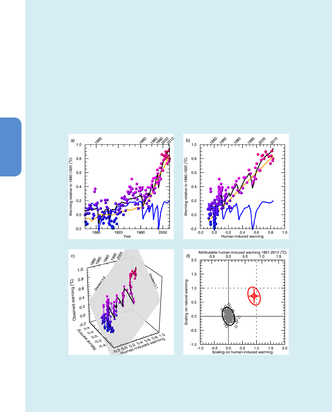
Box 10.1 | How Attribution Studies Work

This box presents an idealized demonstration of the concepts underlying most current approaches to detection and attribution of cli-

mate change and how these relate to conventional linear regression. The coloured dots in Box 10.1a, Figure 1 show observed annual

GMST from 1861 to 2012, with warmer years coloured red and colder years coloured blue. Observations alone indicate, unequivocally,

that the Earth has warmed, but to quantify how different external factors have contributed to this warming, studies must compare

such observations with the expected responses to these external factors. The orange line shows an estimate of the GMST response to

anthropogenic (GHG and aerosol) forcing obtained from the mean of the CMIP3 and CMIP5 ensembles, while the blue line shows the

CMIP3/CMIP5 ensemble mean response to natural (solar and volcanic) forcing.

In statistical terms, attribution involves ﬁnding the combination of these anthropogenic and natural responses that best ﬁts these

observations: this is shown by the black line in panel (a). To show how this ﬁt is obtained in non-technical terms, the data are plotted

against model-simulated anthropogenic warming, instead of time, in panel (b). There is a strong correlation between observed temper-

atures and model-simulated anthropogenic warming, but because of the presence of natural factors and internal climate variability,

correlation alone is not enough for attribution.

To quantify how much of the observed warming is attributable to human inﬂuence, panel (c) shows observed temperatures plotted

against the model-simulated response to anthropogenic forcings in one direction and natural forcings in the other. Observed tempera-

tures increase with both natural and anthropogenic model-simulated warming: the warmest years are in the far corner of the box. A

ﬂat surface through these points (here obtained by an ordinary least-squares ﬁt), indicated by the coloured mesh, slopes up away from

the viewer.

The orientation of this surface indicates how model-simulated responses to natural and anthropogenic forcing need to be scaled to

reproduce the observations. The best-ﬁt gradient in the direction of anthropogenic warming (visible on the rear left face of the box) is

0.9, indicating the CMIP3/CMIP5 ensemble average overestimates the magnitude of the observed response to anthropogenic forcing

by about 10%. The best-ﬁt gradient in the direction of natural changes (visible on the rear right face) is 0.7, indicating that the observed

response to natural forcing is 70% of the average model-simulated response. The black line shows the points on this ﬂat surface that

are directly above or below the observations: each ‘pin’ corresponds to a different year. When re-plotted against time, indicated by the

years on the rear left face of the box, this black line gives the black line previously seen in panel (a). The length of the pins indicates

‘residual’ temperature ﬂuctuations due to internal variability.

The timing of these residual temperature ﬂuctuations is unpredictable, representing an inescapable source of uncertainty. We can

quantify this uncertainty by asking how the gradients of the best-ﬁt surface might vary if El Niño events, for example, had occurred

in different years in the observed temperature record. To do this, we repeat the analysis in panel (c), replacing observed temperatures

with samples of simulated internal climate variability from control runs of coupled climate models. Grey diamonds in panel (d) show

the results: these gradients cluster around zero, because control runs have no anthropogenic or natural forcing, but there is still some

scatter. Assuming that internal variability in global temperature simply adds to the response to external forcing, this scatter provides an

estimate of uncertainty in the gradients, or scaling factors, required to reproduce the observations, shown by the red cross and ellipse.

The red cross and ellipse are clearly separated from the origin, which means that the slope of the best-ﬁt surface through the obser-

vations cannot be accounted for by internal variability: some climate change is detected in these observations. Moreover, it is also

separated from both the vertical and horizontal axes, which means that the responses to both anthropogenic and natural factors are

individually detectable.

The magnitude of observed temperature change is consistent with the CMIP3/CMIP5 ensemble average response to anthropogenic

forcing (uncertainty in this scaling factor spans unity) but is signiﬁcantly lower than the model-average response to natural forcing (this

5 to 95% conﬁdence interval excludes unity). There are, however, reasons why these models may be underestimating the response to

volcanic forcing (e.g., Driscoll et al, 2012), so this discrepancy does not preclude detection and attribution of both anthropogenic and

natural inﬂuence, as simulated by the CMIP3/CMIP5 ensemble average, in the observed GMST record.

The top axis in panel (d) indicates the attributable anthropogenic warming over 1951–2010, estimated from the anthropogenic warm-

ing in the CMIP3/CMIP5 ensemble average, or the gradient of the orange line in panel (a) over this period. Because the model-simulat-

ed responses have been scaled to ﬁt the observations, the attributable anthropogenic warming in this example is 0.6°C to 0.9°C and

does not depend on the magnitude of the raw model-simulated changes. Hence an attribution statement based on such an analysis,

(continued on next page)

876

Chapter 10 Detection and Attribution of Climate Change: from Global to Regional

Box 10.1 (continued)

such as ‘most of the warming over the past 50 years is attributable to anthropogenic drivers’, depends only on the shape, or time his-

tory, not the size, of the model-simulated warming, and hence does not depend on the models’ sensitivity to rising GHG levels.

Formal attribution studies like this example provide objective estimates of how much recent warming is attributable to human inﬂu-

ence. Attribution is not, however, a purely statistical exercise. It also requires an assessment that there are no confounding factors that

could have caused a large part of the ‘attributed’ change. Statistical tests can be used to check that observed residual temperature

ﬂuctuations (the lengths and clustering of the pins in panel (c)) are consistent with internal variability expected from coupled models,

but ultimately these tests must complement physical arguments that the combination of responses to anthropogenic and natural forc-

ing is the only available consistent explanation of recent observed temperature change.

This demonstration assumes, for visualization purposes, that there are only two candidate contributors to the observed warming,

anthropogenic and natural, and that only GMST is available. More complex attribution problems can be undertaken using the same

principles, such as aiming to separate the response to GHGs from other anthropogenic factors by also including spatial information.

These require, in effect, an extension of panel (c), with additional dimensions corresponding to additional causal factors, and additional

points corresponding to temperatures in different regions.

Box 10.1, Figure 1 | Example of a simpliﬁed detection and attribution study. (a) Observed global annual mean temperatures relative to 1880–1920 (coloured dots)

compared with CMIP3/CMIP5 ensemble-mean response to anthropogenic forcing (orange), natural forcing (blue) and best-ﬁt linear combination (black). (b) As (a) but

all data plotted against model-simulated anthropogenic warming in place of time. Selected years (increasing nonlinearly) shown on top axis. (c) Observed temperatures

versus model-simulated anthropogenic and natural temperature changes, with best-ﬁt plane shown by coloured mesh. (d) Gradient of best-ﬁt plane in (c), or scaling on

model-simulated responses required to ﬁt observations (red diamond) with uncertainty estimate (red ellipse and cross) based on CMIP5 control integrations (grey dia-

monds). Implied attributable anthropogenic warming over the period 1951–2010 is indicated by the top axis. Anthropogenic and natural responses are noise-reduced

with 5-point running means, with no smoothing over years with major volcanoes.

877

Detection and Attribution of Climate Change: from Global to Regional Chapter 10

series properties (notice how date information is effectively discarded

in panel (b) of Box 10.1, Figure 1) and require fewer assumptions about

the stationarity of the input series.

All of these approaches are subject to the issue of confounding fac-

tors identiﬁed by Hegerl and Zwiers (2011). For example, Beenstock et

al. (2012) fail to ﬁnd a consistent co-integrating relationship between

atmospheric carbon dioxide (CO

) concentrations and GMST using pol-

ynomial cointegration tests, but the fact that CO

concentrations are

derived from different sources in different periods (ice cores prior to the

mid-20th-century, atmospheric observations thereafter) makes it difﬁ-

cult to assess the physical signiﬁcance of their result, particularly in the

light of evidence for co-integration between temperature and radiative

forcing (RF) reported by Kaufmann et al. (2011) using tests of linear

cointegration, and also the results of Gay-Garcia et al. (2009), who ﬁnd

evidence for external forcing of climate using time series properties.

The assumptions of the statistical model employed can also inﬂuence

results. For example, Schlesinger and Ramankutty (1994) and Zhou

and Tung (2013a) show that GMST are consistent with a linear anthro-

pogenic trend, enhanced variability due to an approximately 70-year

Atlantic Meridional Oscillation (AMO) and shorter-term variability. If,

however, there are physical grounds to expect a nonlinear anthropo-

genic trend (see Box 10.1 Figure 1a), the assumption of a linear trend

can itself enhance the variance assigned to a low-frequency oscillation.

The fact that the AMO index is estimated from detrended historical tem-

perature observations further increases the risk that its variance may

be overestimated, because regressors and regressands are not inde-

pendent. Folland et al. (2013), using a physically based estimate of the

anthropogenic trend, ﬁnd a smaller role for the AMO in recent warming.

Time series methods ultimately depend on the structural adequacy of

the statistical model employed. Many such studies, for example, use

models that assume a single exponential decay time for the response

to both external forcing and stochastic ﬂuctuations. This can lead to

an overemphasis on short-term ﬂuctuations, and is not consistent with

the response of more complex models (Knutti et al., 2008). Smirnov and

Mokhov (2009) propose an alternative characterization that allows

them to distinguish a ‘long-term causality’ that focuses on low-fre-

quency changes. Trends that appear signiﬁcant when tested against

an AR(1) model may not be signiﬁcant when tested against a process

that supports this ‘long-range dependence’ (Franzke, 2010). Although

the evidence for long-range dependence in global temperature data

remains a topic of debate (Mann, 2011; Rea et al., 2011) , it is generally

desirable to explore sensitivity of results to the speciﬁcation of the sta-

tistical model, and also to other methods of estimating the properties

of internal variability, such as more complex climate models, discussed

next. For example, Imbers et al. (2013) demonstrate that the detection

of the inﬂuence of increasing GHGs in the global temperature record

is robust to the assumption of a Fractional Differencing (FD) model of

internal variability, which supports long-range dependence.

10.2.3 Methods Based on General Circulation Models

and Optimal Fingerprinting

Fingerprinting methods use climate model simulations to provide

more complete information about the expected response to different

external drivers, including spatial information, and the properties of

internal climate variability. This can help to separate patterns of forced

change both from each other and from internal variability. The price,

however, is that results depend to some degree on the accuracy of the

shape of model-simulated responses to external factors (e.g., North

and Stevens, 1998), which is assessed by comparing results obtained

with expected responses estimated from different climate models.

When the signal-to-noise (S/N) ratio is low, as can be the case for

some regional indicators and some variables other than temperature,

the accuracy of the speciﬁcation of variability becomes a central factor

in the reliability of any detection and attribution study. Many studies

of such variables inﬂate the variability estimate from models to deter-

mine if results are sensitive to, for example, doubling of variance in the

control (e.g., Zhang et al., 2007), although Imbers et al. (2013) note

that errors in the spectral properties of simulated variability may also

be important.

A full description of optimal ﬁngerprinting is provided in Appendix 9.A

of Hegerl et al. (2007b) and further discussion is to be found in Hassel-

mann (1997), Allen and Tett (1999), Allen et al. (2006), and Hegerl and

Zwiers (2011). Box 10.1 provides a simple example of ‘ﬁngerprinting’

based on GMST alone. In a typical ﬁngerprint analysis, model-simu-

lated spatio-temporal patterns of response to different combinations

of external forcings, including segments of control integrations with

no forcing, are ‘observed’ in a similar manner to the historical record

(masking out times and regions where observations are absent). The

magnitudes of the model-simulated responses are then estimated in

the observations using a variant of linear regression, possibly allowing

for signals being contaminated by internal variability (Allen and Stott,

2003) and structural model uncertainty (Huntingford et al., 2006).

In ‘optimal’ ﬁngerprinting, model-simulated responses and observa-

tions are normalized by internal variability to improve the S/N ratio.

This requires an estimate of the inverse noise covariance estimated

from the sample covariance matrix of a set of unforced (control) sim-

ulations (Hasselmann, 1997), or from variations within an initial-con-

dition ensemble. Because these control runs are generally too short

to estimate the full covariance matrix, a truncated version is used,

retaining only a small number, typically of order 10 to 20, of high-vari-

ance principal components. Sensitivity analyses are essential to ensure

results are robust to this, relatively arbitrary, choice of truncation (Allen

and Tett, 1999; Ribes and Terray, 2013; Jones et al., 2013 ). Ribes et

al. (2009) use a regularized estimate of the covariance matrix, mean-

ing a linear combination of the sample covariance matrix and a unit

matrix that has been shown (Ledoit and Wolf, 2004) to provide a more

accurate estimate of the true covariance, thereby avoiding dependence

on truncation. Optimization of S/N ratio is not, however, essential for

many attribution results (see, e.g., Box 10.1) and uncertainty analysis

in conventional optimal ﬁngerprinting does not require the covariance

matrix to be inverted, so although regularization may help in some

cases, it is not essential. Ribes et al. (2010) also propose a hybrid of

the model-based optimal ﬁngerprinting and time series approaches,

referred to as ‘temporal optimal detection’, under which each signal is

assumed to consist of a single spatial pattern modulated by a smoothly

varying time series estimated from a climate model (see also Santer et

al., 1994).

878

Chapter 10 Detection and Attribution of Climate Change: from Global to Regional

The ﬁnal statistical step in an attribution study is to check that the

residual variability, after the responses to external drivers have been

estimated and removed, is consistent with the expected properties of

internal climate variability, to ensure that the variability used for uncer-

tainty analysis is realistic, and that there is no evidence that a potential-

ly confounding factor has been omitted. Many studies use a standard

F-test of residual consistency for this purpose (Allen and Tett, 1999).

Ribes et al. (2013) raise some issues with this test, but key results are

not found to be sensitive to different formulations. A more important

issue is that the F-test is relatively weak (Berliner et al., 2000; Allen et

al., 2006; Terray, 2012), so ‘passing’ this test is not a safeguard against

unrealistic variability, which is why estimates of internal variability are

discussed in detail in this chapter and in Chapter 9.

A further consistency check often used in optimal ﬁngerprinting is

whether the estimated magnitude of the externally driven responses

are consistent between model and observations (scaling factors con-

sistent with unity in Box 10.1): if they are not, attribution is still possi-

ble provided the discrepancy is explicable in terms of known uncertain-

ties in the magnitude of either forcing or response. As is emphasized

in Section 10.2.1 and Box 10.1, attribution is not a purely statistical

assessment: physical judgment is required to assess whether the com-

bination of responses considered allows for all major potential con-

founding factors and whether any remaining discrepancies are consist-

ent with a physically based understanding of the responses to external

forcing and internal climate variability.

10.2.4 Single-Step and Multi-Step Attribution and the

Role of the Null Hypothesis

Attribution studies have traditionally involved explicit simulation of

the response to external forcing of an observable variable, such as sur-

face temperature, and comparison with corresponding observations of

that variable. This so-called ‘single-step attribution’ has the advantage

of simplicity, but restricts attention to variables for which long and

consistent time series of observations are available and that can be

simulated explicitly in current models driven solely with external cli-

mate forcing.

To address attribution questions for variables for which these condi-

tions are not satisﬁed, Hegerl et al. (2010) introduced the notation of

‘multi-step attribution’, formalizing existing practice (e.g., Stott et al.,

2004). In a multi-step attribution study, the attributable change in a

variable such as large-scale surface temperature is estimated with a

single-step procedure, along with its associated uncertainty, and the

implications of this change are then explored in a further (physically

or statistically based) modelling step. Overall conclusions can only be

as robust as the least certain link in the multi-step procedure. As the

focus shifts towards more noisy regional changes, it can be difﬁcult

to separate the effect of different external forcings. In such cases, it

can be useful to detect the response to all external forcings, and then

determine the most important factors underlying the attribution results

by reference to a closely related variable for which a full attribution

analysis is available (e.g., Morak et al., 2011).

Attribution results are typically expressed in terms of conventional ‘fre-

quentist’ conﬁdence intervals or results of hypothesis tests: when it is

reported that the response to anthropogenic GHG increase is very likely

greater than half the total observed warming, it means that the null

hypothesis that the GHG-induced warming is less than half the total

can be rejected with the data available at the 10% signiﬁcance level.

Expert judgment is required in frequentist attribution assessments, but

its role is limited to the assessment of whether internal variability and

potential confounding factors have been adequately accounted for,

and to downgrade nominal signiﬁcance levels to account for remaining

uncertainties. Uncertainties may, in some cases, be further reduced if

prior expectations regarding attribution results themselves are incor-

porated, using a Bayesian approach, but this not currently the usual

practice.

This traditional emphasis on single-step studies and placing lower

bounds on the magnitude of signals under investigation means that,

very often, the communication of attribution results tends to be con-

servative, with attention focussing on whether or not human inﬂuence

in a particular variable might be zero, rather than the upper end of the

conﬁdence interval, which might suggest a possible response much

bigger than current model-simulated changes. Consistent with previous

Assessments and the majority of the literature, this chapter adopts this

conservative emphasis. It should, however, be borne in mind that this

means that positive attribution results will tend to be biased towards

well-observed, well-modelled variables and regions, which should be

taken into account in the compilation of global impact assessments

(Allen, 2011; Trenberth, 2011a).

10.3 Atmosphere and Surface

This section assesses causes of change in the atmosphere and at the

surface over land and ocean.

10.3.1 Temperature

Temperature is ﬁrst assessed near the surface of the Earth in Section

10.3.1.1 and then in the free atmosphere in Section 10.3.1.2.

10.3.1.1 Surface (Air Temperature and Sea Surface Temperature)

10.3.1.1.1 Observations of surface temperature change

GMST warmed strongly over the period 1900–1940, followed by a

period with little trend, and strong warming since the mid-1970s (Sec-

tion 2.4.3, Figure 10.1). Almost all observed locations have warmed

since 1901 whereas over the satellite period since 1979 most regions

have warmed while a few regions have cooled (Section 2.4.3; Figure

10.2). Although this picture is supported by all available global

near-surface temperature data sets, there are some differences in

detail between them, but these are much smaller than both interan-

nual variability and the long-term trend (Section 2.4.3). Since 1998

the trend in GMST has been small (see Section 2.4.3, Box 9.2). Urban-

ization is unlikely to have caused more than 10% of the measured

centennial trend in land mean surface temperature, though it may have

contributed substantially more to regional mean surface temperature

trends in rapidly developing regions (Section 2.4.1.3).

879

Detection and Attribution of Climate Change: from Global to Regional Chapter 10

10.3.1.1.2 Simulations of surface temperature change

As discussed in Section 10.1, the CMIP5 simulations have several

advantages compared to the CMIP3 simulations assessed by (Hegerl et

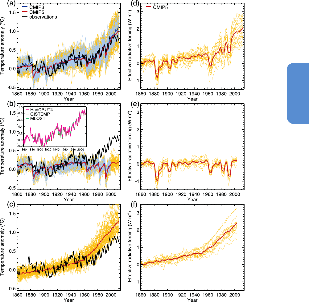
al., 2007b) for the detection and attribution of climate change. Figure

10.1a shows that when the effects of anthropogenic and natural exter-

nal forcings are included in the CMIP5 simulations the spread of sim-

Figure 10.1 | (Left-hand column) Three observational estimates of global mean surface temperature (GMST, black lines) from Hadley Centre/Climatic Research Unit gridded surface

temperature data set 4 (HadCRUT4), Goddard Institute of Space Studies Surface Temperature Analysis (GISTEMP), and Merged Land–Ocean Surface Temperature Analysis (MLOST),

compared to model simulations [CMIP3 models – thin blue lines and CMIP5 models – thin yellow lines] with anthropogenic and natural forcings (a), natural forcings only (b) and

greenhouse gas (GHG) forcing only (c). Thick red and blue lines are averages across all available CMIP5 and CMIP3 simulations respectively. CMIP3 simulations were not avail-

able for GHG forcing only (c). All simulated and observed data were masked using the HadCRUT4 coverage (as this data set has the most restricted spatial coverage), and global

average anomalies are shown with respect to 1880–1919, where all data are ﬁrst calculated as anomalies relative to 1961–1990 in each grid box. Inset to (b) shows the three

observational data sets distinguished by different colours. (Adapted from Jones et al., 2013.) (Right-hand column) Net adjusted forcing in CMIP5 models due to anthropogenic and

natural forcings (d), natural forcings only (e) and GHGs only (f). (From Forster et al., 2013.) Individual ensemble members are shown by thin yellow lines, and CMIP5 multi-model

means are shown as thick red lines.

ulated GMST anomalies spans the observational estimates of GMST

anomaly in almost every year whereas this is not the case for simu-

lations in which only natural forcings are included (Figure 10.1b) (see

also Jones et al., 2013; Knutson et al., 2013). Anomalies are shown

relative to 1880–1919 rather than absolute temperatures. Showing

anomalies is necessary to prevent changes in observational cover-

age being reﬂected in the calculated global mean and is reasonable

880

Chapter 10 Detection and Attribution of Climate Change: from Global to Regional

because climate sensitivity is not a strong function of the bias in GMST

in the CMIP5 models (Section 9.7.1; Figure 9.42). Simulations with GHG

changes only, and no changes in aerosols or other forcings, tend to sim-

ulate more warming than observed (Figure 10.1c), as expected. Better

agreement between models and observations when the models include

anthropogenic forcings is also seen in the CMIP3 simulations (Figure

10.1, thin blue lines). RF in the simulations including anthropogenic

and natural forcings differs considerably among models (Figure 10.1d),

and forcing differences explain much of the differences in temperature

response between models over the historical period (Forster et al., 2013

). Differences between observed GMST based on three observational

data sets are small compared to forced changes (Figure 10.1).

As discussed in Section 10.2, detection and attribution assessments

are more robust if they consider more than simple consistency argu-

ments. Analyses that allow for the possibility that models might be

consistently over- or underestimating the magnitude of the response

to climate forcings are assessed in Section 10.3.1.1.3, the conclusions

from which are not affected by evidence that model spread in GMST

in CMIP3, is smaller than implied by the uncertainty in RF (Schwartz

et al., 2007). Although there is evidence that CMIP3 models with a

higher climate sensitivity tend to have a smaller increase in RF over

the historical period (Kiehl, 2007; Knutti, 2008; Huybers, 2010), no

such relationship was found in CMIP5 (Forster et al., 2013 ) which

may explain the wider spread of the CMIP5 ensemble compared to

the CMIP3 ensemble (Figure 10.1a). Climate model parameters are

typically chosen primarily to reproduce features of the mean climate

and variability (Box 9.1), and CMIP5 aerosol emissions are standard-

ized across models and based on historical emissions (Lamarque et

al., 2010; Section 8.2.2), rather than being chosen by each modelling

group independently (Curry and Webster, 2011; Hegerl et al., 2011c).

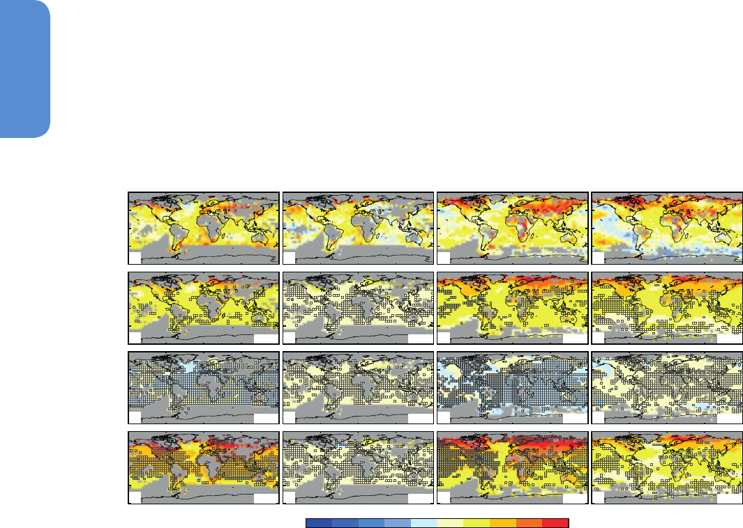
Figure 10.2a shows the pattern of annual mean surface temperature

trends observed over the period 1901–2010, based on Hadley Centre/

Climatic Research Unit gridded surface temperature data set 4 (Had-

CRUT4). Warming has been observed at almost all locations with sufﬁ-

cient observations available since 1901. Rates of warming are general-

ly higher over land areas compared to oceans, as is also apparent over

the 1951–2010 period (Figure 10.2c), which simulations indicate is

due mainly to differences in local feedbacks and a net anomalous heat

transport from oceans to land under GHG forcing, rather than differ-

ences in thermal inertia (e.g., Boer, 2011). Figure 10.2e demonstrates

that a similar pattern of warming is simulated in the CMIP5 simula-

tions with natural and anthropogenic forcing over the 1901–2010

period. Over most regions, observed trends fall between the 5th and

95th percentiles of simulated trends, and van Oldenborgh et al. (2013)

ﬁnd that over the 1950–2011 period the pattern of observed grid cell

trends agrees with CMIP5 simulated trends to within a combination of

-90 0 90 180

-180 -90 0 90 180

-90

-45

21%

15%

32%

14%

-90

-45

48%

69%

44%

89%

-90

-45

22%

43%

46%

50%

-90

-45

-2 -1 012

Trend (°C per period)

1901-2010 1901-1950 1951-2010 1979-2010

HadCRUT4historicalhistoricalNathistoricalGHG

Figure 10.2 | Trends in observed and simulated temperatures (K over the period shown) over the 1901–2010 (a, e, i, m), 1901–1950 (b, f, j, n), 1951–2010 (c, g, k, o) and

1979–2010 (d, h, l, p) periods. Trends in observed temperatures from the Hadley Centre/Climatic Research Unit gridded surface temperature data set 4 (HadCRUT4) (a–d), CMIP3

and CMIP5 model simulations including anthropogenic and natural forcings (e–h), CMIP3 and CMIP5 model simulations including natural forcings only (i–l) and CMIP3 and CMIP5

model simulations including greenhouse gas forcing only (m–p). Trends are shown only where sufﬁcient observational data are available in the HadCRUT4 data set, and grid cells

with insufﬁcient observations to derive trends are shown in grey. Boxes in (e–p) show where the observed trend lies outside the 5 to 95th percentile range of simulated trends,

and the ratio of the number of such grid cells to the total number of grid cells with sufﬁcient data is shown as a percentage in the lower right of each panel. (Adapted from Jones

et al., 2013.)

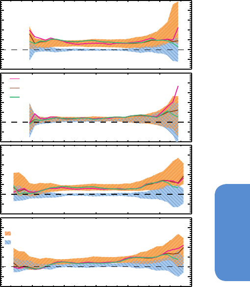
881

Detection and Attribution of Climate Change: from Global to Regional Chapter 10

-2

-1

(°C per 110 years)

90S 60S 30S 0 30N 60N 90N

1901-2010

(a)

-2

-1

(°C per 50 years)

1901-1950

HadCRUT4

GISTEMP

MLOST

(b)

-2

-1

(°C per 60 years)

1951-2010

(c)

-2

-1

(°C per 32 years)

1979-2010

90S 60S 30S 0 30N 60N 90N

Latitude

(d)

historical 5-95% range

historicalNat 5-95% range

model spread and internal variability. Areas of disagreement over the

1901–2010 period include parts of Asia and the Southern Hemisphere

(SH) mid-latitudes, where the simulations warm less than the obser-

vations, and parts of the tropical Paciﬁc, where the simulations warm

more than the observations (Jones et al., 2013; Knutson et al., 2013).

Stronger warming in observations than models over parts of East Asia

could in part be explained by uncorrected urbanization inﬂuence in the

observations (Section 2.4.1.3), or by an overestimate of the response

to aerosol increases. Trends simulated in response to natural forcings

only are generally close to zero, and inconsistent with observed trends

in most locations (Figure 10.2i) (see also Knutson et al., 2013). Trends

simulated in response to GHG changes only over the 1901–2010

period are larger than those observed at most locations, and in many

cases signiﬁcantly so (Figure 10.2m). This is expected because these

simulations do not include the cooling effects of aerosols. Differenc-

es in patterns of simulated and observed seasonal mean temperature

trends and possible causes are considered in more detail in Box 11.2.

Over the period 1979–2010 most observed regions exhibited warming

(Figure 10.2d), but much of the eastern Paciﬁc and Southern Oceans

cooled. These regions of cooling are not seen in the simulated trends

over this period in response to anthropogenic and natural forcing

(Figure 10.2h), which show signiﬁcantly more warming in much of

these regions (Jones et al., 2013; Knutson et al., 2013). This cooling

and reduced warming in observations over the Southern Hemisphere

mid-latitudes over the 1979–2010 period can also be seen in the zonal

mean trends (Figure 10.3d), which also shows that the models tend to

warm too much in this region over this period. However, there is no dis-

crepancy in zonal mean temperature trends over the longer 1901–2010

period in this region (Figure 10.3a), suggesting that the discrepancy

over the 1979–2010 period either may be an unusually strong manifes-

tation of internal variability in the observations or relate to regionally

important forcings over the past three decades which are not included

in most CMIP5 simulations, such as sea salt aerosol increases due to

strengthened high latitude winds (Korhonen et al., 2010), or sea ice

extent increases driven by freshwater input from ice shelf melting (Bin-

tanja et al., 2013). Except at high latitudes, zonal mean trends over the

1901–2010 period in all three data sets are inconsistent with natural-

ly forced trends, indicating a detectable anthropogenic signal in most

zonal means over this period (Figure 10.3a). McKitrick and Tole (2012)

ﬁnd that few CMIP3 models have signiﬁcant explanatory power when

ﬁtting the spatial pattern of 1979–2002 trends in surface temperature

over land, by which they mean that these models add little or no skill

to a ﬁt including the spatial pattern of tropospheric temperature trends

as well as the major atmospheric oscillations. This is to be expected,

as temperatures in the troposphere are well correlated in the vertical,

and local temperature trends over so short a period are dominated by

internal variability.

CMIP5 models generally exhibit realistic variability in GMST on decadal

to multi-decadal time scales (Jones et al., 2013; Knutson et al., 2013;

Section 9.5.3.1, Figure 9.33), although it is difﬁcult to evaluate internal

variability on multi-decadal time scales in observations given the short-

ness of the observational record and the presence of external forcing.

The observed trend in GMST since the 1950s is very large compared to

model estimates of internal variability (Stott et al., 2010; Drost et al.,

2012; Drost and Karoly, 2012). Knutson et al. (2013) compare observed

trends in GMST with a combination of simulated internal variability

and the response to natural forcings and ﬁnd that the observed trend

would still be detected for trends over this period even if the magni-

tude of the simulated natural variability (i.e., the standard deviation of

trends) were tripled.

10.3.1.1.3 Attribution of observed global-scale temperature

changes

The evolution of temperature since the start of the global

instrumental record

Since the AR4, detection and attribution studies have been carried out

using new model simulations with more realistic forcings, and new

observational data sets with improved representation of uncertainty

(Christidis et al., 2010; Jones et al., 2011, 2013; Gillett et al., 2012,

2013; Stott and Jones, 2012; Knutson et al., 2013; Ribes and Terray,

2013). Although some inconsistencies between the simulated and

observed responses to forcings in individual models were identiﬁed

( Gillett et al., 2013; Jones et al., 2013; Ribes and Terray, 2013) over-

Figure 10.3 | Zonal mean temperature trends over the 1901–2010 (a), 1901–1950

(b), 1951–2010 (c) and 1979–2010 (d) periods. Solid lines show Hadley Centre/Cli-

matic Research Unit gridded surface temperature data set 4 (HadCRUT4, red), God-

dard Institute of Space Studies Surface Temperature Analysis (GISTEMP, brown) and

Merged Land–Ocean Surface Temperature Analysis (MLOST, green) observational data

sets, orange hatching represents the 90% central range of CMIP3 and CMIP5 simula-

tions with anthropogenic and natural forcings, and blue hatching represents the 90%

central range of CMIP3 and CMIP5 simulations with natural forcings only. All model

and observations data are masked to have the same coverage as HadCRUT4. (Adapted

from Jones et al., 2013.)

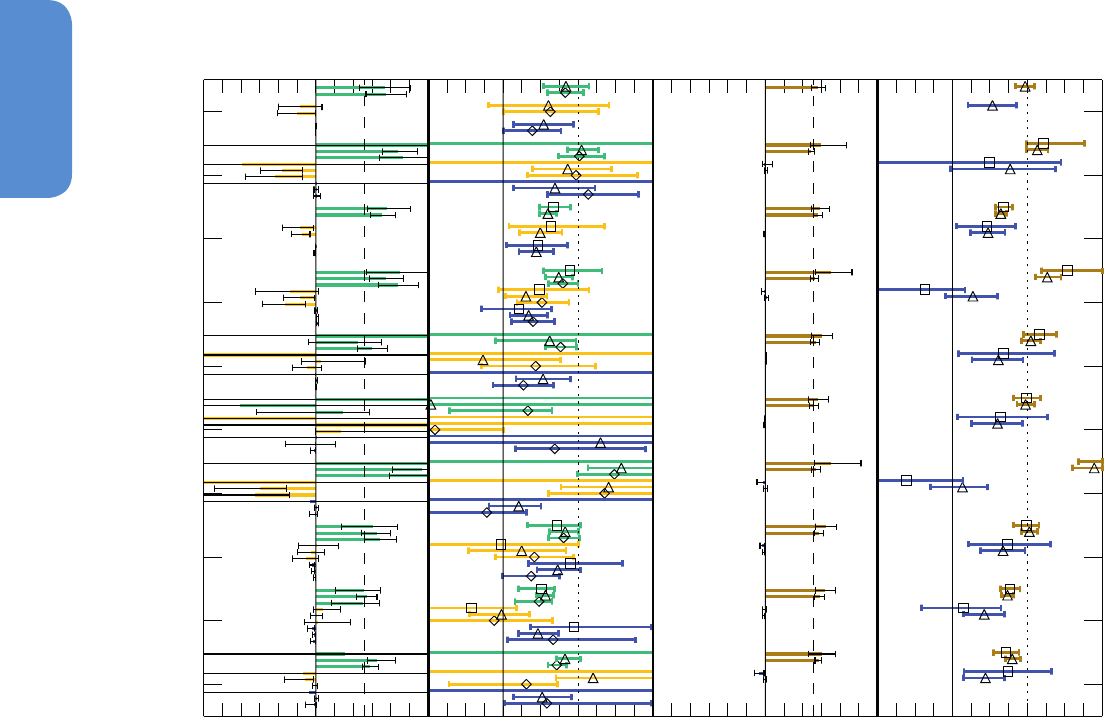
882

Chapter 10 Detection and Attribution of Climate Change: from Global to Regional

all these results support the AR4 assessment that GHG increases very

likely caused most (>50%) of the observed GMST increase since the

mid-20th century (Hegerl et al., 2007b).

The results of multiple regression analyses of observed temperature

changes onto the simulated responses to GHG, other anthropogen-

ic and natural forcings are shown in Figure 10.4 (Gillett et al., 2013;

Jones et al., 2013; Ribes and Terray, 2013). The results, based on Had-

CRUT4 and a multi-model average, show robustly detected responses

to GHG in the observational record whether data from 1861–2010 or

only from 1951–2010 are analysed (Figure 10.4b). The advantage of

analysing the longer period is that more information on observed and

modelled changes is included, while a disadvantage is that it is difﬁcult

to validate climate models’ estimates of internal variability over such

a long period. Individual model results exhibit considerable spread

among scaling factors, with estimates of warming attributable to each

forcing sensitive to the model used for the analsys (Figure 10.4; Gillett

-1 0 1 -0.5 0 0.5 1 1.5 -1 0 1 -0.5 0 0.5 1 1.5

(°C per 60 years) (°C per 60 years)

BCC-CSM1-1

CanESM2

CNRM-CM5

CSIRO-Mk3-6-0

GISS-E2-H

GISS-E2-R

HadGEM2-ES

IPSL-CM5A-LR

NorESM1-M

multi

BCC-CSM1-1

CanESM2

CNRM-CM5

CSIRO-Mk3-6-0

GISS-E2-H

GISS-E2-R

HadGEM2-ES

IPSL-CM5A-LR

NorESM1-M

multi

1951-2010 trend Scaling factor 1951-2010 trend Scaling factor

(a) (b) (c) (d)

Scaling factor Scaling factor

et al., 2013; Jones et al., 2013; Ribes and Terray, 2013), the period over

which the analysis is applied (Figure 10.4; Gillett et al., 2013; Jones et

al., 2013), and the Empirical Orthogonal Function (EOF) truncation or

degree of spatial ﬁltering (Jones et al., 2013; Ribes and Terray, 2013).

In some cases the GHG response is not detectable in regressions using

individual models (Figure 10.4; Gillett et al., 2013; Jones et al., 2013;

Ribes and Terray, 2013), or a residual test is failed (Gillett et al., 2013;

Jones et al., 2013; Ribes and Terray, 2013), indicating a poor ﬁt between

the simulated response and observed changes. Such cases are proba-

bly due largely to errors in the spatio-temporal pattern of responses

to forcings simulated in individual models (Ribes and Terray, 2013),

although observational error and internal variability errors could also

play a role. Nonetheless, analyses in which responses are averaged

across multiple models generally show much less sensitivity to period

and EOF trucation (Gillett et al., 2013; Jones et al., 2013), and more

consistent residuals (Gillett et al., 2013), which may be because model

response errors are smaller in a multi-model mean.

Figure 10.4 | (a) Estimated contributions of greenhouse gas (GHG, green), other anthropogenic (yellow) and natural (blue) forcing components to observed global mean surface

temperature (GMST) changes over the 1951–2010 period. (b) Corresponding scaling factors by which simulated responses to GHG (green), other anthropogenic (yellow) and

natural forcings (blue) must be multiplied to obtain the best ﬁt to Hadley Centre/Climatic Research Unit gridded surface temperature data set 4 (HadCRUT4; Morice et al., 2012)

observations based on multiple regressions using response patterns from nine climate models individually and multi-model averages (multi). Results are shown based on an analysis

over the 1901–2010 period (squares, Ribes and Terray, 2013), an analysis over the 1861–2010 period (triangles, Gillett et al., 2013) and an analysis over the 1951–2010 period

(diamonds, Jones et al., 2013). (c, d) As for (a) and (b) but based on multiple regressions estimating the contributions of total anthropogenic forcings (brown) and natural forcings

(blue) based on an analysis over 1901–2010 period (squares, Ribes and Terray, 2013) and an analysis over the 1861–2010 period (triangles, Gillett et al., 2013). Coloured bars

show best estimates of the attributable trends (a and c) and 5 to 95% conﬁdence ranges of scaling factors (b and d). Vertical dashed lines in (a) and (c) show the best estimate

HadCRUT4 observed trend over the period concerned. Vertical dotted lines in (b) and d) denote a scaling factor of unity.

883

Detection and Attribution of Climate Change: from Global to Regional Chapter 10

We derive assessed ranges for the attributable contributions of GHGs,

other anthropogenic forcings and natural forcings by taking the small-

est ranges with a precision of one decimal place that span the 5 to

95% ranges of attributable trends over the 1951–2010 period from

the Jones et al. (2013) weighted multi-model analysis and the Gillett

et al. (2013) multi-model analysis considering observational uncer-

tainty (Figure 10.4a). The assessed range for the attributable contri-

bution of combined anthropogenic forcings was derived in the same

way from the Gillett et al. (2013) multi-model attributable trend and

shown in Figure 10.4c. We moderate our likelihood assessment and

report likely ranges rather than the very likely ranges directly implied

by these studies in order to account for residual sources of uncertainty

including sensitivity to EOF truncation and analysis period (e.g., Ribes

and Terray, 2013). In this context, GHGs means well-mixed greenhouse

gases (WMGHGs), other anthropogenic forcings means aerosol chang-

es, and in most models ozone changes and land use changes, and nat-

ural forcings means solar irradiance changes and volcanic aerosols.

Over the 1951–2010 period, the observed GMST increased by approx-

imately 0.6°C. GHG increases likely contributed 0.5°C to 1.3°C, other

anthropogenic forcings likely contributed –0.6°C to 0.1°C and natural

forcings likely contributed –0.1°C to 0.1°C to observed GMST trends

over this period. Internal variability likely contributed –0.1°C to 0.1°C

to observed trends over this period (Knutson et al., 2013). This assess-

ment is shown schematically in Figure 10.5. The assessment is support-

ed additionally by a complementary analysis in which the parameters

of an Earth System Model of Intermediate Complexity (EMIC) were

constrained using observations of near-surface temperature and ocean

heat content, as well as prior information on the magnitudes of forc-

ings, and which concluded that GHGs have caused 0.6°C to 1.1°C (5

to 95% uncertainty) warming since the mid-20th century (Huber and

Knutti, 2011); an analysis by Wigley and Santer (2013), who used an

energy balance model and RF and climate sensitivity estimates from

AR4, and they concluded that there was about a 93% chance that

GHGs caused a warming greater than observed over the 1950–2005

period; and earlier detection and attribution studies assessed in the

AR4 (Hegerl et al., 2007b).

The inclusion of additional data to 2010 (AR4 analyses stopped at

1999; Hegerl et al. (2007b)) helps to better constrain the magnitude of

the GHG-attributable warming (Drost et al., 2012; Gillett et al., 2012;

Stott and Jones, 2012; Gillett et al., 2013), as does the inclusion of

spatial information (Stott et al., 2006; Gillett et al., 2013), though Ribes

and Terray (2013) caution that in some cases there are inconsistencies

between observed spatial patterns of response and those simulated in

indvidual models. While Hegerl et al. (2007b) assessed that a signiﬁcant

cooling of about 0.2 °C was attributable to natural forcings over the

1950–1999 period, the temperature trend attributable to natural forc-

ings over the 1951–2010 period is very small (<0.1°C). This is because,

while Mt Pinatubo cooled global temperatures in the early 1990s,

there have been no large volcanic eruptions since, resulting in small

simulated trends in response to natural forcings over the 1951–2010

period (Figure 10.1b). Regression coefﬁcients for natural forcings tend

to be smaller than one, suggesting that the response to natural forc-

ings may be overestimated by the CMIP5 models on average (Figure

10.4; Gillett et al., 2013; Knutson et al., 2013). Attribution of observed

changes is robust to observational uncertainty which is comparably

important to internal climate variability as a source of uncertainty in

GHG-attributable warming and aerosol-attributable cooling (Jones and

Stott, 2011; Gillett et al., 2013; Knutson et al., 2013). The response to

GHGs was detected using Hadley Centre new Global Environmental

Model 2-Earth System (HadGEM2-ES; Stott and Jones, 2012), Canadian

Earth System Model 2 (CanESM2; Gillett et al., 2012) and other CMIP5

models except for Goddard Institute for Space Studies-E2-H (GISS-

E2-H; Gillett et al., 2013; Jones et al., 2013) (Figure 10.4). However, the

inﬂuence of other anthropogenic forcings was detected only in some

CMIP5 models (Figure 10.4). This lack of detection of other anthro-

pogenic forcings compared to detection of an aerosol response using

four CMIP3 models over the period 1900–1999 (Hegerl et al., 2007b)

does not only relate to the use of data to 2010 rather than 2000 (Stott

and Jones, 2012), although this could play a role (Gillett et al., 2013;

Ribes and Terray, 2013). Whether it is associated with a cancellation of

aerosol cooling by ozone and black carbon (BC) warming in the CMIP5

simulations, making the signal harder to detect, or by some aspect of

the response to other anthropogenic forcings that is less realistic in

these models is not clear.

Although closely constraining the GHG and other anthropogenic con-

tributions to observed warming remains challenging owing to their

degeneracy and sensitivity to methodological choices (Jones et al.,

2013; Ribes and Terray, 2013), a total anthropogenic contribution to

warming can be much more robustly constrained by a regression of

observed temperature changes onto the simulated responses to all

anthropogenic forcings and natural forcings (Figure 10.4; Gillett et

al., 2013; Ribes and Terray, 2013). Robust detection of anthropogenic

inﬂuence is also found if a new optimal detection methodology, the

Regularised Optimal Fingerprint approach (see Section 10.2; Ribes et

al., 2013), is applied (Ribes and Terray, 2013). A better constrained

estimate of the total anthropogenic contribution to warming since the

mid-20th century than the GHG contribution is also found by Wigley

and Santer (2013). Knutson et al. (2013) demonstrate that observed

trends in GMST are inconsistent with the simulated response to natural

forcings alone, but consistent with the simulated response to natural

and anthropogenic forcings for all periods beginning between 1880

and 1990 and ending in 2010, which they interpret as evidence that

warming is in part attributable to anthropogenic inﬂuence over these

periods. Based on the well-constrained attributable anthropogenic

trends shown in Figure 10.4 we assess that anthropogenic forcings

likely contributed 0.6°C to 0.8°C to the observed warming over the

1951–2010 period (Figure 10.5).

There are some inconsistencies in the simulated and observed magni-

tudes of responses to forcing for some CMIP5 models (Figure 10.4); for

example, CanESM2 has a GHG regression coefﬁcient signiﬁcantly less

than 1 and a regression coefﬁcient for other anthropogenic forcings

also signiﬁcantly less than 1 (Gillett et al., 2012; Gillett et al., 2013;

Jones et al., 2013; Ribes and Terray, 2013), indicating that this model

overestimates the magnitude of the response to GHGs and to other

anthropogenic forcings. Averaged over the ensembles of models con-

sidered by Gillett et al. (2013) and Jones et al. (2013), the best-estimate

GHG and OA scaling factors are less than 1 (Figure 10.4), indicating

that the model mean GHG and OA responses should be scaled down

to best match observations. The best-estimate GHG scaling factors are

larger than the best-estimate OA scaling factors, although the discrep-

ancy from 1 is not signiﬁcant in either case and the ranges of the GHG

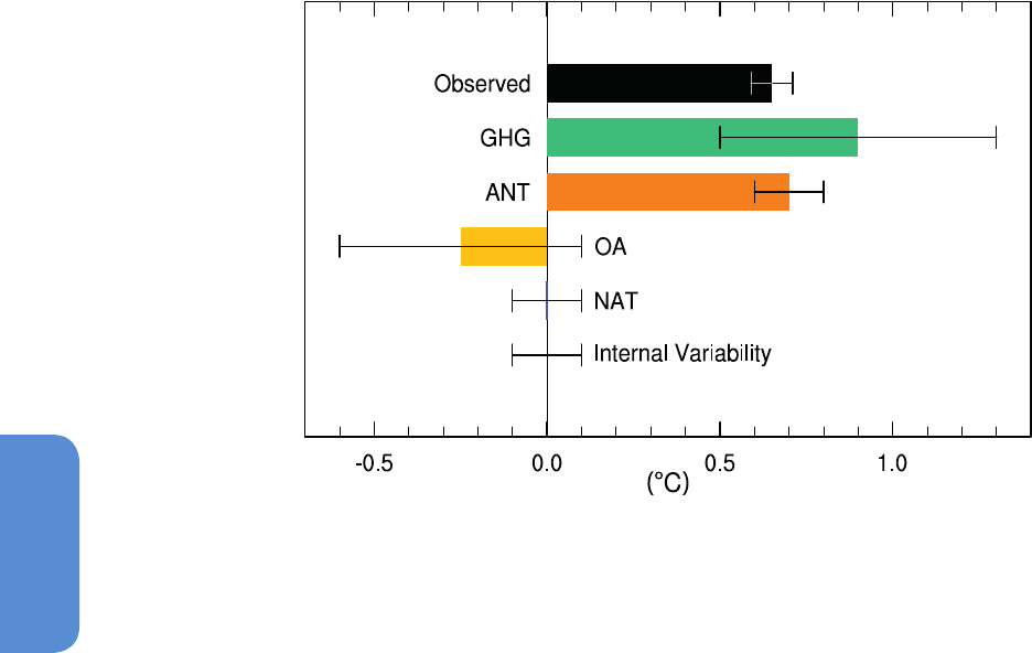
884

Chapter 10 Detection and Attribution of Climate Change: from Global to Regional

Figure 10.5 | Assessed likely ranges (whiskers) and their mid-points (bars) for attributable warming trends over the 1951–2010 period due to well-mixed greenhouse gases, other

anthropogenic forcings (OA), natural forcings (NAT), combined anthropogenic forcings (ANT) and internal variability. The Hadley Centre/Climatic Research Unit gridded surface

temperature data set 4 (HadCRUT4) observations are shown in black with the 5 to 95% uncertainty range due to observational uncertainty in this record (Morice et al., 2012).

and OA scaling factors are overlapping. Overall there is some evidence

that some CMIP5 models have a higher transient response to GHGs

and a larger response to other anthropogenic forcings (dominated by

the effects of aerosols) than the real world (medium conﬁdence). Incon-

sistencies between simulated and observed trends in GMST were also

identiﬁed in several CMIP3 models by Fyfe et al. (2010) after remov-

ing volcanic, El Niño-Southern Oscillation (ENSO), and Cold Ocean/

Warm Land pattern (COWL) signals from GMST, although uncertainties

may have been underestimated because residuals were modelled by

a ﬁrst-order autoregressive processes. A longer observational record

and a better understanding of the temporal changes in forcing should

make it easier to identify discrepancies between the magnitude of the

observed response to a forcing, and the magnitude of the response

simulated in individual models. To the extent that inconsistencies

between simulated and observed changes are independent between

models, this issue may be addressed by basing our assessment on attri-

bution analyses using the mean response from multiple models, and

by accounting for model uncertainty when making such assessments.

In conclusion, although some inconsistencies in the forced respons-

es of individual models and observations have been identiﬁed, the

detection of the global temperature response to GHG increases using

average responses from multiple models is robust to observational

uncertainty and methodological choices. It is supported by basic phys-

ical arguments. We conclude, consistent with Hegerl et al. (2007b),

that more than half of the observed increase in GMST from 1951 to

2010 is very likely due to the observed anthropogenic increase in GHG

concentrations.

The inﬂuence of BC aerosols (from fossil and biofuel sources) has

been detected in the recent global temperature record in one analy-

sis, although the warming attributable to BC by Jones et al. (2011) is

small compared to that attributable to GHG increases. This warming is

simulated mainly over the Northern Hemisphere (NH) with a sufﬁcient-

ly distinct spatio-temporal pattern that it could be separated from the

response to other forcings in this study.

Several recent studies have used techniques other than regres-

sion-based detection and attribution analyses to address the causes

of recent global temperature changes. Drost and Karoly (2012)

demonstrated that observed GMST, land–ocean temperature con-

trast, meridional temperature gradient and annual cycle amplitude

exhibited trends over the period 1956–2005 that were outside the 5

to 95% range of simulated internal variability in eight CMIP5 models,

based on three different observational data sets. They also found that

observed trends in GMST and land–ocean temperature contrast were

larger than those simulated in any of 36 CMIP5 simulations with nat-

ural forcing only. Drost et al. (2012) found that 1961–2010 trends in

GMST and land–ocean temperature contrast were signiﬁcantly larger

than simulated internal variability in eight CMIP3 models. By compar-

ing observed GMST with simple statistical models, Zorita et al. (2008)

concluded that there is a very low probability that observed clustering

of very warm years in the last decade occurred by chance. Smirnov and

Mokhov (2009), adopting an approach that allowed them to distin-

guish between conventional Granger causality and a ‘long-term cau-

sality’ that focuses on low-frequency changes (see Section 10.2), found

that increasing CO

concentrations are the principal determining factor

in the rise of GMST over recent decades. Sedlacek and Knutti (2012)

found that the spatial patterns of sea surface temperature (SST) trends

from simulations forced with increases in GHGs and other anthropo-

genic forcings agree well with observations but differ from warming

patterns associated with internal variability.

Several studies that have aimed to separate forced surface temper-

ature variations from those associated with internal variability have

identiﬁed the North Atlantic as a dominant centre of multi-decadal

885

Detection and Attribution of Climate Change: from Global to Regional Chapter 10

internal variability, and in particular modes of variability related to

the Atlantic Multi-decadal Oscillation (AMO; Section 14.7.6). The AMO

index is deﬁned as an area average of North Atlantic SSTs, and it has

an apparent period of around 70 years, which is long compared to

the length of observational record making it difﬁcult to deduce robust

conclusions about the role of the AMO from only two cycles. Never-

theless, several studies claim a role for internal variability associated

with the AMO in driving enhanced warming in the 1980s and 1990s

as well as the recent slow down in warming (Box 9.2), while attribut-

ing long-term warming to anthropogenically forced variations either

by analysing time series of GMST, forcings and indices of the AMO

(Rohde et al., 2013; Tung and Zhou, 2013; Zhou and Tung, 2013a) or by

analysing both spatial and temporal patterns of temperature (Swan-

son et al., 2009; DelSole et al., 2011; Wu et al., 2011). Studies based

on global mean time series could risk falsely attributing variability to

the AMO when variations in external forcings, for example, associated

with aerosols, could also cause similar variability. In contrast, studies

using space–time patterns seek to distinguish the spatialstructure of

temperature anomalies associated with the AMO from those associat-

ed with forced variability. Unforced climate simulations indicate that

internal multi-decadal variability in the Atlantic is characterized by

surface anomalies of the same sign from the equator to the high lat-

itudes,with maximum amplitudes in subpolar regions (Delworth and

Mann, 2000; Latif et al., 2004; Knight et al., 2005; DelSole et al., 2011)

while the net response to anthropogenic and naturalforcing over the

20th century, such as observed temperature change, is characterized

by warming nearly everywhere onthe globe, but with minimum warm-

ing or even cooling in the subpolar regions of the NorthAtlantic (Figure

10.2; Ting et al., 2009; DelSole et al., 2011).

Some studies implicate tropospheric aerosols in driving decadal var-

iations in Atlantic SST (Evan et al., 2011; Booth et al., 2012; Terray,

2012), and temperature variations in eastern North America (Leibens-

perger et al., 2012). Booth et al. (2012) ﬁnd that most multi-decadal

variability in North Atlantic SSTs is simulated in one model mainly in

response to aerosol variations, although its simulated changes in North

Atlantic ocean heat content and salinity have been shown to be incon-

sistent with observations (Zhang et al., 2012). To the extent that cli-

mate models simulate realistic internal variability in the AMO (Section

9.5.3.3.2), AMO variability is accounted for in uncertainty estimates

from regression-based detection and attribution studies (e.g., Figure

10.4).

To summarize, recent studies using spatial features of observed tem-

perature variations to separate AMO variability from externally forced

changes ﬁnd that detection of external inﬂuence on global tempera-

tures is not compromised by accounting for AMO-congruent variability

(high conﬁdence). There remains some uncertainty about how much

decadal variability of GMST that is attributed to AMO in some studies

is actually related to forcing, notably from aerosols. There is agree-

ment among studies that the contribution of the AMO to global warm-

ing since 1951 is very small (considerably less than 0.1°C; see also

Figure 10.6) and given that observed warming since 1951 is very large

compared to climate model estimates of internal variability (Section

10.3.1.1.2), which are assessed to be adequate at global scale (Section

9.5.3.1), we conclude that it is virtually certain that internal variability

alone cannot account for the observed global warming since 1951.

Box 10.2 | The Sun’s Inﬂuence on the Earth’s Climate

A number of studies since AR4 have addressed the possible inﬂuences of long-term ﬂuctuations of solar irradiance on past climates,

particularly related to the relative warmth of the Medieval Climate Anomaly (MCA) and the relative coolness in the Little Ice Age (LIA).

There is medium conﬁdence that both external solar and volcanic forcing, and internal variability, contributed substantially to the spa-

tial patterns of surface temperature changes between the MCA and the LIA, but very low conﬁdence in quantitative estimates of their

relative contributions (Sections 5.3.5.3 and 5.5.1). The combined inﬂuence of volcanism, solar forcing and a small drop in greenhouse

gases (GHGs) likely contributed to Northern Hemisphere cooling during the LIA (Section 10.7.2). Solar radiative forcing (RF) from the

Maunder Minimum (1745) to the satellite era (average of 1976–2006) has been estimated to be +0.08 to +0.18 W m

–2

(low conﬁdence,

Section 8.4.1.2). This may have contributed to early 20th century warming (low conﬁdence, Section 10.3.1).

More recently, it is extremely unlikely that the contribution from solar forcing to the observed global warming since 1950 was larger

than that from GHGs (Section 10.3.1.1.3). It is very likely that there has been a small decrease in solar forcing of –0.04 [–0.08 to 0.00]

W m

–2

over a period with direct satellite measurements of solar output from 1986 to 2008 (Section 8.4.1.1). There is high conﬁdence

that changes in total solar irradiance have not contributed to global warming during that period.

Since AR4, there has been considerable new research that has connected solar forcing to climate. The effect of solar forcing on GMST

trends has been found to be small, with less than 0.1°C warming attributable to combined solar and volcanic forcing over the 1951–

2010 period (Section 10.3.1), although the 11-year cycle of solar variability has been found to have some inﬂuence on GMST variability

over the 20th century. GMST changes between solar maxima and minima are estimated to be of order 0.1°C from some regression

studies of GMST and forcing estimates (Figure 10.6), although several studies have suggested these results may be too large owing to

issues including degeneracy between forcing and with internal variability, overﬁtting of forcing indices and underestimated uncertain-

ties in responses (Ingram, 2007; Benestad and Schmidt, 2009; Stott and Jones, 2009). Climate models generally show less than half this

variability (Jones et al., 2012). (continued on next page)

886

Chapter 10 Detection and Attribution of Climate Change: from Global to Regional

Box 10.2 (continued)

Variability associated with the 11-year solar cycle has also been shown to produce measurable short-term regional and seasonal

climate anomalies (Miyazaki and Yasunari, 2008; Gray et al., 2010; Lockwood, 2012; National Research Council, 2012) particularly in

the Indo-Paciﬁc, Northern Asia and North Atlantic regions (medium evidence). For example, studies have suggested an 11-year solar

response in the Indo-Paciﬁc region in which the equatorial eastern Paciﬁc sea surface temperatures (SSTs) tend to be below normal,

the sea level pressure (SLP) in the Gulf of Alaska and the South Paciﬁc above normal, and the tropical convergence zones on both

hemispheres strengthened and displaced polewards under solar maximum conditions, although it can be difﬁcult to discriminate the

solar-forced signal from the El Niño-Southern Oscillation (ENSO) signal (van Loon et al., 2007; van Loon and Meehl, 2008; White and Liu,

2008; Meehl and Arblaster, 2009; Roy and Haigh, 2010, 2012; Tung and Zhou, 2010; Bal et al., 2011; Haam and Tung, 2012; Hood and

Soukharev, 2012; Misios and Schmidt, 2012). For northern summer, there is evidence that for peaks in the 11-year solar cycle, the Indian

monsoon is intensiﬁed (Kodera, 2004; van Loon and Meehl, 2012), with solar variability affecting interannual connections between

the Indian and Paciﬁc sectors due to a shift in the location of the descending branch of the Walker Circulation (Kodera et al., 2007). In

addition, model sensitivity experiments (Ineson et al., 2011) suggest that the negative phase of the North Atlantic Oscillation (NAO) is

more prevalent during solar minima and there is some evidence of this in observations, including an indication of increased frequency

of high-pressure ‘blocking’ events over Europe in winter (Barriopedro et al., 2008; Lockwood et al., 2010; Woollings et al., 2010).

Two mechanisms have been identiﬁed in observations and simulated with climate models that could explain these low amplitude

regional responses (Gray et al., 2010; medium evidence). These mechanisms are additive and may reinforce one another so that the

response to an initial small change in solar irradiance is ampliﬁed regionally (Meehl et al., 2009). The ﬁrst mechanism is a top-down

mechanism ﬁrst noted by Haigh (1996) where greater solar ultraviolet radiation (UV) in peak solar years warms the stratosphere direct-

ly via increased radiation and indirectly via increased ozone production. This can result in a chain of processes that inﬂuences deep

tropical convection (Balachandran et al., 1999; Shindell et al., 1999; Kodera and Kuroda, 2002; Haigh et al., 2005; Kodera, 2006; Matthes

et al., 2006). In addition, there is less heating than average in the tropical upper stratosphere under solar minimum conditions which

weakens the equator-to-pole temperature gradient. This signal can propagate downward to weaken the tropospheric mid-latitude

westerlies, thus favoring a negative phase of the Arctic Oscillation (AO) or NAO. This response has been shown in several models (e.g.,

Shindell et al., 2001; Ineson et al., 2011) though there is no signiﬁcant AO or NAO response to solar irradiance variations on average in

the CMIP5 models (Gillett and Fyfe, 2013).

The second mechanism is a bottom-up mechanism that involves coupled air–sea radiative processes in the tropical and subtropical Pacif-

ic that also inﬂuence convection in the deep tropics (Meehl et al., 2003, 2008; Rind et al., 2008; Bal et al., 2011; Cai and Tung, 2012; Zhou

and Tung, 2013b). Such mechanisms have also been shown to inﬂuence regional temperatures over longer time scales (decades to cen-

turies), and can help explain patterns of regional temperature changes seen in paleoclimate data (e.g., Section 10.7.2; Mann et al., 2009;

Goosse et al., 2012b) although they have little effect on global or hemispheric mean temperatures at either short or long time scales.

A possible amplifying mechanism linking solar variability and the Earth’s climate system via cosmic rays has been postulated. It is

proposed that variations in the cosmic ray ﬂux associated with changes in solar magnetic activity affect ion-induced aerosol nucleation

and cloud condensation nuclei (CCN) production in the troposphere (Section 7.4.6). A strong solar magnetic ﬁeld would deﬂect cosmic

rays and lead to fewer CCN and less cloudiness, thereby allowing for more solar energy into the system. Since AR4, there has been

further evidence to disprove the importance of this amplifying mechanism. Correlations between cosmic ray ﬂux and observed aerosol

or cloud properties are weak and local at best, and do not prove to be robust on the regional or global scale (Section 7.4.6). Although

there is some evidence that ionization from cosmic rays may enhance aerosol nucleation in the free troposphere, there is medium evi-

dence and high agreement that the cosmic ray–ionization mechanism is too weak to inﬂuence global concentrations of CCN or their

change over the last century or during a solar cycle in any climatically signiﬁcant way (Sections 7.4.6 and 8.4.1.5). The lack of trend in

cosmic ray intensity over the 1960–2005 period (McCracken and Beer, 2007) provides another argument against the hypothesis of a

major contribution of cosmic ray variations to the observed warming over that period given the existence of short time scales in the

climate system response.

Thus, although there is medium conﬁdence that solar variability has made contributions to past climate ﬂuctuations, since the mid-

20th century there has been little trend in solar forcing. There are at least two amplifying mechanisms that have been proposed and

simulated in some models that could explain small observed regional and seasonal climate anomalies associated with the 11-year solar

cycle, mostly in the Indo-Paciﬁc region and northern mid to high latitudes.

Regarding possible future inﬂuences of the sun on the Earth’s climate, there is very low conﬁdence in our ability to predict future solar

output, but there is high conﬁdence that the effects from solar irradiance variations will be much smaller than the projected climate

changes from increased RF due to GHGs (Sections 8.4.1.3 and 11.3.6.2.2).

887

Detection and Attribution of Climate Change: from Global to Regional Chapter 10

Based on a range of detection and attribution analyses using multi-

ple solar irradiance reconstructions and models, Hegerl et al. (2007b)

concluded that it is very likely that GHGs caused more global warming

than solar irradiance variations over the 1950–1999 period. Detection

and attribution analyses applied to the CMIP5 simulations (Figure

10.4) indicate less than 0.1°C temperature change attributable to com-

bined solar and volcanic forcing over the 1951–2010 period. Based on

a regression of paleo temperatures onto the response to solar forc-

ing simulated by an energy balance model, Scafetta and West (2007)

ﬁnd that up to 50% of the warming since 1900 may be solar-induced,

but Benestad and Schmidt (2009) show this conclusion is not robust,

being based on disregarding forcings other than solar in the prein-

dustrial period, and assuming a high and precisely known value for

climate sensitivity. Despite claims that more than half the warming

since 1970 can be ascribed to solar variability (Loehle and Scaffetta,

2011) , a conclusion based on an incorrect assumption of no anthro-

pogenic inﬂuence before 1950 and a 60-year solar cycle inﬂuence on

global temperature (see also Mazzarella and Scafetta, 2012), several

studies show that solar variations cannot explain global mean surface

warming over the past 25 years, because solar irradiance has declined

over this period (Lockwood and Fröhlich, 2007, 2008; Lockwood, 2008,

2012 ). Lean and Rind (2008) conclude that solar forcing explains only

10% of the warming over the past 100 years, while contributing a

small cooling over the past 25 years. Thus while there is some evidence

for solar inﬂuences on regional climate variability (Box 10.2) solar forc-

ing has only had a small effect on GMST. Overall, we conclude that it

is extremely unlikely that the contribution from solar forcing to the

warming since 1950 was larger than that from GHGs.

A range of studies have used statistical methods to separate out the

inﬂuence of known sources of internal variability, including ENSO

and, in some cases, the AMO, from the response to external drivers,

including volcanoes, solar variability and anthropogenic inﬂuence,

in the recent GMST record: see, for example, Lockwood (2008), Lean

and Rind (2009), Folland et al. (2013 ), Foster and Rahmstorf (2011)

and Kaufmann et al. (2011). Representative results, as summarized in

Imbers et al. (2013), are shown in Figure 10.6. These consistently attrib-

ute most of the warming over the past 50 years to anthropogenic inﬂu-

ence, even allowing for potential confounding factors like the AMO.

While results of such statistical approaches are sensitive to assump-

tions regarding the properties of both responses to external drivers and

internal variability (Imbers et al., 2013), they provide a complementary

approach to attribution studies based on global climate models.

Overall, given that the anthropogenic increase in GHGs likely caused

0.5°C to 1.3°C warming over 1951–2010, with other anthropogenic

forcings probably contributing counteracting cooling, that the effects

of natural forcings and natural internal variability are estimated to be

small, and that well-constrained and robust estimates of net anthropo-

genic warming are substantially more than half the observed warming

(Figure 10.4) we conclude that it is extremely likely that human activ-

ities caused more than half of the observed increase in GMST from

1951 to 2010.

The early 20th century warming

The instrumental GMST record shows a pronounced warming during

the ﬁrst half of the 20th century (Figure 10.1a). Correction of residual

biases in SST observations leads to a higher estimate of 1950s temper-

atures, but does not substantially change the warming between 1900

and 1940 (Morice et al., 2012). The AR4 concluded that ‘the early 20th

century warming is very likely in part due to external forcing’ (Hegerl

et al., 2007b), and that it is likely that anthropogenic forcing contrib-

uted to this warming. This assessment was based on studies including

Shiogama et al. (2006) who ﬁnd a contribution from solar and volcanic

forcing to observed warming to 1949, and Min and Hense (2006), who

ﬁnd strong evidence for a forced (either natural or combined natu-

ral and anthropogenic) contribution to global warming from 1900 to

1949. Ring et al. (2012) estimate, based on time series analysis, that

part of the early 20th century warming was due to GHG increases (see

also Figure 10.6), but ﬁnd a dominant contribution by internal varia-

bility. CMIP5 model simulations of the historical period show forced

warming over the early 20th century (Figure 10.1a), consistent with

earlier detection and attribution analyses highlighted in the AR4 and

TAR. The early 20th century contributes to the detection of external

forcings over the 20th century estimated by detection and attribution

results (Figure 10.4; Gillett et al., 2013; Ribes and Terray, 2013) and

to the detected change over the last millennium to 1950 (see Figure

10.19; Schurer et al., 2013).

The pattern of warming and residual differences between models and

observations indicate a role for circulation changes as a contributor to

early 20th cenury warming (Figure 10.2), and the contribution of internal

variability to the early 20th century warming has been analysed in sev-

eral publications since the AR4. Crook and Forster (2011) ﬁnd that the

observed 1918–1940 warming was signiﬁcantly greater than that simu-

lated by most of the CMIP3 models. A distinguishing feature of the early

20th century warming is its pattern (Brönnimann, 2009) which shows

the most pronounced warming in the Arctic during the cold season, fol-

lowed by North America during the warm season, the North Atlantic

Ocean and the tropics. In contrast, there was no unusual warming in

Australia among other regions (see Figure 10.2b). Such a pronounced

pattern points to a role for circulation change as a contributing factor

to the regional anomalies contributing to this warming. Some studies

have suggested that the warming is a response to the AMO (Schlesinger

and Ramankutty, 1994; Polyakov et al., 2005; Knight et al., 2006; Tung

and Zhou, 2013), or a large but random expression of internal variability

(Bengtsson et al., 2006; Wood and Overland, 2010). Knight et al. (2009)

diagnose a shift from the negative to the positive phase of the AMO

from 1910 to 1940, a mode of circulation that is estimated to contribute

approximately 0.1°C, trough to peak, to GMST (Knight et al., 2005).

Nonetheless, these studies do not challenge the AR4 assessment that

external forcing very likely made a contribution to the warming over this

period. In conclusion, the early 20th century warming is very unlikely to

be due to internal variability alone. It remains difﬁcult to quantify the

contribution to this warming from internal variability, natural forcing

and anthropogenic forcing, due to forcing and response uncertainties

and incomplete observational coverage.

Year-to-year and decade-to-decade variability of global mean

surface temperature

Time series analyses, such as those shown in Figure 10.6, seek to par-

tition the variability of GMST into components attributable to anthro-

pogenic and natural forcings and modes of internal variability such

as ENSO and the AMO. Although such time series analyses support

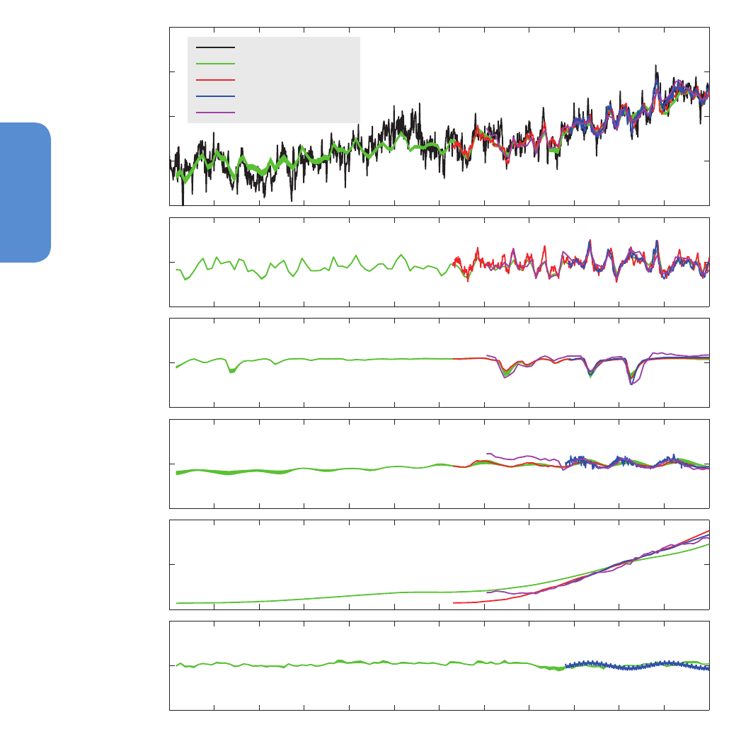
888

Chapter 10 Detection and Attribution of Climate Change: from Global to Regional

the major role of anthropogenic forcings, particularly due to increasing

GHG concentrations, in contributing to the overall warming over the

last 60 years, many factors, in addition to GHGs, including changes

in tropospheric and stratospheric aerosols, stratospheric water vapour

and solar output, as well as internal modes of variability, contribute

to the year-to-year and decade-to-decade variability of GMST (Figure

10.6). Detailed discussion of the evolution of GMST of the past 15

years since 1998 is contained in Box 9.2.

−1

−0.5

0.5

Obs. & reconstructions (°C)

Estimated contributions to global mean temperature change

All temperatures relative to 1980−2000

HadCRUT3 observations

Folland

Lean

Kaufmann

Lockwood

−0.5

0.5

ENSO (°C)

−0.5

0.5

Volcanoes (°C)

−0.5

0.5

Solar (°C)

−0.5

0.5

Anthropogenic (°C)

1890 1900 1910 1920 1930 1940 1950 1960 1970 1980 1990 2000 2010

−0.5

0.5

AMO and other (°C)

Figure 10.6 | (Top) The variations of the observed global mean surface temperature (GMST) anomaly from Hadley Centre/Climatic Research Unit gridded surface temperature data

set version 3 (HadCRUT3, black line) and the best multivariate ﬁts using the method of Lean (red line), Lockwood (pink line), Folland (green line) and Kaufmann (blue line). (Below)

The contributions to the ﬁt from (a) El Niño-Southern Oscillation (ENSO), (b) volcanoes, (c) solar forcing, (d) anthropogenic forcing and (e) other factors (Atlantic Multi-decadal

Oscillation (AMO) for Folland and a 17.5-year cycle, semi-annual oscillation (SAO), and Arctic Oscillation (AO) from Lean). (From Lockwood (2008), Lean and Rind (2009), Folland

et al. (2013 ) and Kaufmann et al. (2011), as summarized in Imbers et al. (2013).)

10.3.1.1.4 Attribution of regional surface temperature change

Anthropogenic inﬂuence on climate has been robustly detected on

the global scale, but for many applications an estimate of the anthro-

pogenic contribution to recent temperature trends over a particular

region is more useful. However, detection and attribution of climate

change at continental and smaller scales is more difﬁcult than on the

global scale for several reasons (Hegerl et al., 2007b; Stott et al., 2010).

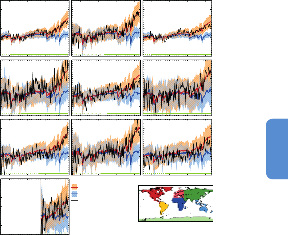
889

Detection and Attribution of Climate Change: from Global to Regional Chapter 10

First, the relative contribution of internal variability compared to the

forced response to observed changes tends to be larger on smaller

scales, as spatial differences in internal variations are averaged out in

large-scale means. Second, because the patterns of response to climate

forcings tend to be large scale, there is less spatial information to help

distinguish between the responses to different forcings when attention

is restricted to a sub-global area. Third, forcings omitted in some global

climate model simulations may be important on regional scales, such

as land use change or BC aerosol. Lastly, simulated internal variability

and responses to forcings may be less reliable on smaller scales than

on the global scale. Knutson et al. (2013) ﬁnd a tendency for CMIP5

models to overestimate decadal variability in the NH extratropics in

individual grid cells and underestimate it elsewhere, although Karoly

and Wu (2005) and Wu and Karoly (2007) ﬁnd that variability is not

generally underestimated in earlier generation models.

Based on several studies, Hegerl et al. (2007b) concluded that ‘it is

likely that there has been a substantial anthropogenic contribution

Temperature anomaly (°C)

-1.0

-0.5

0.0

0.5

1.0

1.5

2.0

1880 1920 1960 2000

Global

1880 1920 1960 2000

Global Land

-1.0

-0.5

0.0

0.5

1.0

1.5

2.0

1880 1920 1960 2000

Global ocean

-1.0

-0.5

0.0

0.5

1.0

1.5

2.0

North America

South America

-1.0

-0.5

0.0

0.5

1.0

1.5

2.0

Europe

-1.0

-0.5

0.0

0.5

1.0

1.5

2.0

Africa

1880 1920 1960 2000

Asia

-1.0

-0.5

0.0

0.5

1.0

1.5

2.0

1880 1920 1960 2000

Australasia

-1.0

-0.5

0.0

0.5

1.0

1.5

2.0

1880 1920 1960 2000

Antarctica

historical 5-95%

historicalNat 5-95%

HadCRUT4

Figure 10.7 | Global, land, ocean and continental annual mean temperatures for CMIP3 and CMIP5 historical (red) and historicalNat (blue) simulations (multi-model means shown

as thick lines, and 5 to 95% ranges shown as thin light lines) and for Hadley Centre/Climatic Research Unit gridded surface temperature data set 4 (HadCRUT4, black). Mean tem-

peratures are shown for Antarctica and six continental regions formed by combining the sub-continental scale regions deﬁned by Seneviratne et al. (2012). Temperatures are shown

with respect to 1880–1919 for all regions apart from Antarctica where temperatures are shown with respect to 1950–2010. (Adapted from Jones et al., 2013.)

to surface temperature increases in every continent except Antarcti-

ca since the middle of the 20th century’. Figure 10.7 shows compari-

sons of observed continental scale temperatures (Morice et al., 2012)

with CMIP5 simulations including both anthropogenic and natural

forcings (red lines) and including just natural forcings (blue lines).

Observed temperatures are largely within the range of simulations

with anthropogenic forcings for all regions and outside the range of

simulations with only natural forcings for all regions except Antarctica

(Jones et al., 2013 ). Averaging over all observed locations, Antarcti-

ca has warmed over the 1950–2008 period (Section 2.4.1.1; Gillett et

al., 2008b; Jones et al., 2013 ), even though some individual locations

have cooled, particularly in summer and autumn, and over the shorter

1960–1999 period (Thompson and Solomon, 2002; Turner et al., 2005).

When temperature changes associated with changes in the South-

ern Annular Mode are removed by regression, both observations and

model simulations indicate warming at all observed locations except

the South Pole over the 1950–1999 period (Gillett et al., 2008b). An

analysis of Antarctic land temperatures over the period 1950–1999

890

Chapter 10 Detection and Attribution of Climate Change: from Global to Regional

detected separate natural and anthropogenic responses of consist-

ent magnitude in simulations and observations (Gillett et al., 2008b).

Thus anthropogenic inﬂuence on climate has now been detected on all

seven continents. However the evidence for human inﬂuence on Ant-

arctic temperature is much weaker than for the other six continental

regions. There is only one attribution study for this region, and there

is greater observational uncertainty than the other regions, with very

few data before 1950, and sparse coverage that is mainly limited to

the coast and the Antarctic Peninsula. As a result of the observational

uncertainties, there is low conﬁdence in Antarctic region land surface

air temperatures changes (Section 2.4.1.1) and we conclude for Ant-

arctica there is low conﬁdence that anthropogenic inﬂuence has con-

tributed to the observed warming averaged over available stations.

Since the publication of the AR4 several other studies have applied

attribution analyses to continental and sub-continental scale regions.

Min and Hense (2007) applied a Bayesian decision analysis technique

to continental-scale temperatures using the CMIP3 multi-model ensem-

ble and concluded that forcing combinations including GHG increases

provide the best explanation of 20th century observed changes in tem-

perature on every inhabited continent except Europe, where the obser-

vational evidence is not decisive in their analysis. Jones et al. (2008)

detected anthropogenic inﬂuence on summer temperatures over all

NH continents and in many subcontinental NH land regions in an

optimal detection analysis that considered the temperature responses

to anthropogenic and natural forcings. Christidis et al. (2010) used a

multi-model ensemble constrained by global-scale observed tempera-

ture changes to estimate the changes in probability of occurrence of

warming or cooling trends over the 1950–1997 period over various

sub-continental scale regions. They concluded that the probability of

occurrence of warming trends had been at least doubled by anthro-

pogenic forcing over all such regions except Central North America.

The estimated distribution of warming trends over the Central North

America region was approximately centred on the observed trend, so

no inconsistency between simulated and observed trends was identi-

ﬁed there. Knutson et al. (2013) demonstrated that observed temper-

ature trends from the beginning of the observational record to 2010

averaged over Europe, Africa, Northern Asia, Southern Asia, Australia

and South America are all inconsistent with the simulated response to

natural forcings alone, and consistent with the simulated response to

combined natural and anthropogenic forcings in the CMIP5 models.

They reached a similar conclusion for the major ocean basins with the

exception of the North Atlantic, where variability is high.

Several recent studies have applied attribution analyses to speciﬁc

sub-continental regions. Anthropogenic inﬂuence has been found in

winter minimum temperature over the western USA (Bonﬁls et al., 2008;

Pierce et al., 2009), a conclusion that is found to be robust to weighting

models according to various aspects of their climatology (Pierce et al.,

2009); anthropogenic inﬂuence has been found in temperature trends

over New Zealand (Dean and Stott, 2009) after circulation-related var-

iability is removed as in Gillett et al. (2000); and anthropogenic inﬂu-

ence has been found in temperature trends over France, using a ﬁrst-or-

der autoregressive model of internal variability (Ribes et al., 2010).

Increases in anthropogenic GHGs were found to be the main driver

of the 20th-century SST increases in both Atlantic and Paciﬁc tropical

cyclogenesis regions (Santer et al., 2006; Gillett et al., 2008a). Over both

regions, the response to anthropogenic forcings is detected when the

response to natural forcings is also included in the analysis (Gillett et al.,

2008a). Knutson et al. (2013) detect an anthropogenic inﬂuence over

Canada, but not over the continental USA, Alaska or Mexico.

Gillett et al. (2008b) detect anthropogenic inﬂuence on near-surface

Arctic temperatures over land, with a consistent magnitude in simu-

lations and observations. Wang et al. (2007) also ﬁnd that observed

Arctic warming is inconsistent with simulated internal variability. Both

studies ascribe Arctic warmth in the 1930s and 1940s largely to inter-

nal variability. Shindell and Faluvegi (2009) infer a large contribution

to both mid-century Arctic cooling and late century warming from

aerosol forcing changes, with GHGs the dominant driver of long-term

warming, though they infer aerosol forcing changes from temperature

changes using an inverse approach which may lead to some changes

associated with internal variability being attributed to aerosol forc-

ing. We therefore conclude that despite the uncertainties introduced

by limited observational coverage, high internal variability, modelling

uncertainties (Crook et al., 2011) and poorly understood local forcings,

such as the effect of BC on snow, there is sufﬁciently strong evidence

to conclude that it is likely that there has been an anthropogenic con-

tribution to the very substantial warming in Arctic land surface temper-

atures over the past 50 years.

Some attribution analyses have considered temperature trends at the

climate model grid box scale. At these spatial scales robust attribu-

tion is difﬁcult to obtain, since climate models often lack the processes

needed to simulate regional details realistically, regionally important

forcings may be missing in some models and observational uncertain-

ties are very large for some regions of the world at grid box scale

(Hegerl et al., 2007b; Stott et al., 2010). Nevertheless an attribution

analysis has been carried out on Central England temperature, a record

that extends back to 1659 and is sufﬁciently long to demonstrate that

the representation of multi-decadal variability in the single grid box in

the model used, Hadley Centre climate prediction model 3 (HadCM3)

is adequate for detection (Karoly and Stott, 2006). The observed trend

in Central England Temperature is inconsistent with either internal var-

iability or the simulated response to natural forcings, but is consistent

with the simulated response when anthropogenic forcings are included

(Karoly and Stott, 2006).

Observed 20th century grid cell trends from Hadley Centre/Climatic

Research Unit gridded surface temperature data set 2v (HadCRUT2v;

Jones et al., 2001) are inconsistent with simulated internal variability

at the 10% signiﬁcance level in around 80% of grid cells even using

HadCM2 which was found to overestimate variability in 5-year mean

temperatures at most latitudes (Karoly and Wu, 2005). Sixty percent of

grid cells were found to exhibit signiﬁcant warming trends since 1951,

a much larger number than expected by chance (Karoly and Wu, 2005;

Wu and Karoly, 2007), and similar results apply when circulation-relat-

ed variability is ﬁrst regressed out (Wu and Karoly, 2007). However, as

discussed in the AR4 (Hegerl et al., 2007b), when a global ﬁeld signiﬁ-

cance test is applied, this becomes a global detection study; since not

all grid cells exhibit signiﬁcant warming trends the overall interpreta-

tion of the results in terms of attribution at individual locations remains

problematic. Mahlstein et al. (2012) ﬁnd signiﬁcant changes in summer

season temperatures in about 40% of low-latitude and about 20% of

891

Detection and Attribution of Climate Change: from Global to Regional Chapter 10

extratropical land grid cells with sufﬁcient observations, when testing

against the null hypothesis of no change in the distribution of summer

temperatures. Observed grid cell trends are compared with CMIP5 sim-

ulated trends in Figure 10.2i, which shows that in the great majority

(89%) of grid cells with sufﬁcient observational coverage, observed

trends over the 1901–2010 period are inconsistent with a combination

of simulated internal variability and the response to natural forcings

(Jones et al., 2013). Knutson et al. (2013) ﬁnd some deﬁciencies in the

simulation of multi-decadal variability at the grid cell scale in CMIP5

models, but demonstrate that trends at more than 75% of individu-

al grid cells with sufﬁcient observational coverage in HadCRUT4 are

inconsistent with the simulated response to natural forcings alone, and

consistent or larger than the simulated response to combined anthro-

pogenic and natural forcings in CMIP5 models.

In summary, it is likely that anthropogenic forcing has made a substan-

tial contribution to the warming of each of the inhabited continents

since 1950. For Antarctica large observational uncertainties result in

low conﬁdence that anthropogenic inﬂuence has contributed to the

observed warming averaged over available stations. Anthropogen-

ic inﬂuence has likely contributed to temperature change in many

sub-continental regions. Detection and attribution of climate change at

continental and smaller scales is more difﬁcult than at the global scale

due to the greater contribution of internal variability, the greater dif-

ﬁculty of distinguishing between different causal factors, and greater

errors in climate models’ representation of regional details. Neverthe-

less, statistically signiﬁcant warming trends are observed at a majority

of grid cells, and the observed warming is inconsistent with estimates

of possible warming due to natural causes at the great majority of grid

cells with sufﬁcient observational coverage.

10.3.1.2 Atmosphere

This section presents an assessment of the causes of global and region-

al temperature changes in the free atmosphere. In AR4, Hegerl et al.

(2007b) concluded that ‘the observed pattern of tropospheric warming

and stratospheric cooling is very likely due to the inﬂuence of anthro-

pogenic forcing, particularly greenhouse gases and stratospheric ozone

depletion.’ Since AR4, insight has been gained into regional aspects of

free tropospheric trends and the causes of observed changes in strat-

ospheric temperature.

Atmospheric temperature trends through the depth of the atmos-

phere offer the possibility of separating the effects of multiple climate

forcings, as climate model simulations indicate that each external

forcing produces a different characteristic vertical and zonal pattern

of temperature response (Hansen et al., 2005b; Hegerl et al., 2007b;

Penner et al., 2007; Yoshimori and Broccoli, 2008). GHG forcing is

expected to warm the troposphere and cool the stratosphere. Strat-

ospheric ozone depletion cools the stratosphere, with the cooling

being most pronounced in the polar regions. Its effect on tropospheric

temperatures is small, which is consistent with a small estimated RF

of stratospheric ozone changes (SPARC CCMVal, 2010; McLandress

et al., 2012). Tropospheric ozone increase, on the other hand, causes

tropospheric warming. Reﬂective aerosols like sulphate cool the trop-

osphere while absorbing aerosols like BC have a warming effect. Free

atmosphere temperatures are also affected by natural forcings: solar

irradiance increases cause a general warming of the atmosphere and

volcanic aerosol ejected into the stratosphere causes tropospheric

cooling and stratospheric warming (Hegerl et al., 2007b).

10.3.1.2.1 Tropospheric temperature change

Chapter 2 concludes that it is virtually certain that globally the tropo-

sphere has warmed since the mid-twentieth century with only medium

(NH extratropics) to low conﬁdence (tropics and SH extratropics) in the

rate and vertical structure of these changes. During the satellite era

CMIP3 and CMIP5 models tend to warm faster than observations spe-

ciﬁcally in the tropics (McKitrick et al., 2010; Fu et al., 2011; Po-Chedley

and Fu, 2012; Santer et al., 2013); however, because of the large uncer-

tainties in observed tropical temperature trends (Section 2.4.4; Seidel

et al. (2012); Figures 2.26 and Figure 2.27) there is only low conﬁdence

in this assessment (Section 9.4.1.4.2). Outside the tropics, and over

the period of the radiosonde record beginning in 1961, the discrep-

ancy between simulated and observed trends is smaller (Thorne et al.,

2011; Lott et al., 2013; Santer et al., 2013). Speciﬁcally there is better

agreement between observed trends and CMIP5 model trends for the

NH extratropics (Lott et al., 2013). Factors other than observational

uncertainties that contribute to inconsistencies between observed and

simulated free troposphere warming include speciﬁc manifestation of

natural variability in the observed coupled atmosphere–ocean system,

forcing errors incorporated in the historical simulations and model

response errors (Santer et al., 2013).

Utilizing a subset of CMIP5 models with single forcing experiments

extending until 2010, Lott et al. (2013) detect inﬂuences of both

human induced GHG increase and other anthropogenic forcings (e.g.,

ozone and aerosols) in the spatio-temporal changes in tropospheric

temperatures from 1961 to 2010 estimated from radiosonde observa-

tions. Figure 10.8 illustrates that a subsample of CMIP5 models (see

Supplementary Material for model selection) forced with both anthro-

pogenic and natural climate drivers (red proﬁles) exhibit trends that

are consistent with radiosonde records in the troposphere up to about

300 hPa, albeit with a tendency for this subset of models to warm more

than the observations. This ﬁnding is seen in near-globally averaged

data (where there is sufﬁcient observational coverage to make a mean-

ingful comparison: 60°S to 60°N) (right panel), as well as in latitudinal

bands of the SH extratropics (Figure 10.8, ﬁrst panel), tropics (Figure

10.8, second panel) and the NH extratropics (Figure 10.8, third panel).

Figure 10.8 also illustrates that it is very unlikely that natural forc-

ings alone could have caused the observed warming of tropospheric

temperatures (blue proﬁles). The ensembles with both anthropogen-

ic and natural forcings (red) and with GHG forcings only (green) are

not clearly separated. This could be due to cancellation of the effects

of increases in reﬂecting aerosols, which cool the troposphere, and

absorbing aerosol (Penner et al., 2007) and tropospheric ozone, which

both warm the troposphere. Above 300 hPa the three radiosonde data

sets exhibit a larger spread as a result of larger uncertainties in the

observational record (Thorne et al., 2011; Section 2.4.4). In this region

of the upper troposphere simulated CMIP5 temperature trends tend

to be more positive than observed trends (Figure 10.8). Further, an

assessment of causes of observed trends in the upper troposphere is

less conﬁdent than an assessment of overall atmospheric temperature

changes because of observational uncertainties and potential remain-

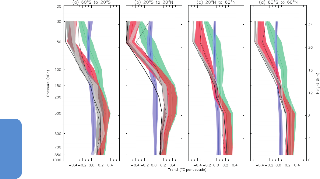
892

Chapter 10 Detection and Attribution of Climate Change: from Global to Regional

ing systematic biases in observational data sets in this region (Thorne

et al., 2011; Haimberger et al., 2012). An analysis of contributions of

natural and anthropogenic forcings to more recent trends from 1979 to

2010 (Supplementary Material, Figure S.A.1) is less robust because of

increased uncertainty in observed trends (consistent with Seidel et al.

(2012)) as well as decreased capability to separate between individual

forcings ensembles.

One approach to identify a climate change signal in a time series is the

analysis of the ratio between the amplitude of the observed signal of

change divided by the magnitude of internal variability, in other words

the S/N ratio of the data record. The S/N ratio represents the result

of a non-optimal ﬁngerprint analysis (in contrast to optimal ﬁnger-

print analyses where model-simulated responses and observations are

normalized by internal variability to improve the S/N ratio (see Section

10.2.3). For changes in the lower stratospheric temperature between

1979 and 2011, S/N ratios vary from 26 to 36, depending on the choice

of observational data set. In the lower troposphere, the ﬁngerprint

strength in observations is smaller, but S/N ratios are still signiﬁcant at

the 1% level or better, and range from 3 to 8. There is no evidence that

these ratios are spuriously inﬂated by model variability errors. After all

global mean signals are removed, model ﬁngerprints remain identiﬁ-

able in 70% of the tests involving tropospheric temperature changes

(Santer et al., 2013).

Hegerl et al. (2007a) concluded that increasing GHGs are the main

cause for warming of the troposphere. This result is supported by a

Figure 10.8 | Observed and simulated zonal mean temperatures trends from 1961 to 2010 for CMIP5 simulations containing both anthropogenic and natural forcings (red),

natural forcings only (blue) and greenhouse gas forcing only (green) where the 5 to 95th percentile ranges of the ensembles are shown. Three radiosonde observations are shown

(thick black line: Hadley Centre Atmospheric Temperature data set 2 (HadAT2), thin black line: RAdiosone OBservation COrrection using REanalyses 1.5 (RAOBCORE 1.5), dark grey

band: Radiosonde Innovation Composite Homogenization (RICH)-obs 1.5 ensemble and light grey: RICH- τ 1.5 ensemble. (After Lott et al., 2013.)

subsample of CMIP5 models that also suggest that the warming effect

of well mixed GHGs is partly offset by the combined effects of reﬂect-

ing aerosols and other forcings. Our understanding has been increased

regarding the time scale of detectability of global scale troposphere

temperature. Taken together with increased understanding of the

uncertainties in observational records of tropospheric temperatures

(including residual systematic biases; Section 2.4.4) the assessment

remains as it was for AR4 that it is likely that anthropogenic forcing has

led to a detectable warming of tropospheric temperatures since 1961.

10.3.1.2.2 Stratospheric temperature change

Lower stratospheric temperatures have not evolved uniformly over

the period since 1958 when the stratosphere has been observed with

sufﬁcient regularity and spatial coverage. A long-term global cooling

trend is interrupted by three 2-year warming episodes following large

volcanic eruptions (Section 2.4.4). During the satellite period the cool-

ing evolved mainly in two steps occurring in the aftermath of the El

Chichón eruption in 1982 and the Mt Pinatubo eruption of 1991, with

each cooling transition being followed by a period of relatively steady

temperatures (Randel et al., 2009; Seidel et al., 2011). Since the mid-

1990s little net change has occurred in lower stratospheric tempera-

tures (Section 2.4.4).

Since AR4, progress has been made in simulating the observed evo-

lution of global mean lower stratospheric temperature. On the one

hand, this has been achieved by using models with an improved

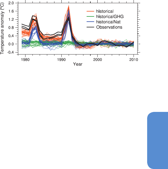
893

Detection and Attribution of Climate Change: from Global to Regional Chapter 10

representation of stratospheric processes (chemistry–climate models

and some CMIP5 models). It is found that in these models which have

an upper boundary above the stratopause with an altitude of about

50 km (so-called high-top models) and improved stratospheric physics,

variability of lower stratosphere climate in general is well simulated

(Butchart et al., 2011; Gillett et al., 2011; Charlton-Perez et al., 2013)

whereas in so-called low-top models (including models participating

in CMIP3) it is generally underestimated (Cordero and Forster, 2006;

Charlton-Perez et al., 2013). On the other hand, CMIP5 models all

include changes in stratospheric ozone (Eyring et al., 2013) whereas

only about half of the models participating in CMIP3 include strato-

spheric ozone changes (Section 9.4.1.4.5). A comparison of a low-top

and high-top version of the HadGEM2 model shows detectable dif-

ferences in modelled temperature changes, particularly in the lower

tropical stratosphere, with the high-top version’s simulation of tem-

perature trends in the tropical troposphere in better agreement with

radiosondes and reanalyses over 1981–2010 (Mitchell et al., 2013).

CMIP5 models forced with changes in WMGHGs and stratospheric

ozone as well as with changes in solar irradiance and volcanic aerosol

forcings simulate the evolution of observed global mean lower strat-

ospheric temperatures over the satellite era reasonably well although

they tend to underestimate the long-term cooling trend (Charlton-Per-

ez et al., 2013; Santer et al., 2013). Compared with radiosonde data the

cooling trend is also underestimated in a subset of CMIP5 simulations

over the period 1961–2010 (Figure 10.8) and in CMIP3 models over

the 1958–1999 period (Cordero and Forster, 2006). Potential causes

for biases in lower stratosphere temperature trends are observational

uncertainties (Section 2.4.4) and forcing errors related to prescribed

stratospheric aerosol loadings and stratospheric ozone changes affect-

ing the tropical lower stratosphere (Free and Lanzante, 2009; Solomon

et al., 2012; Santer et al., 2013).

Since AR4, attribution studies have improved our knowledge of the

role of anthropogenic and natural forcings in observed lower strato-

spheric temperature change. Gillett et al. (2011) use the suite of chem-

istry climate model simulations carried out as part of the Chemistry

Climate Model Validation (CCMVal) activity phase 2 for an attribution

study of observed changes in stratospheric zonal mean temperatures.

Chemistry–climate models prescribe changes in ozone-depleting sub-

stances (ODS) and ozone changes are calculated interactively. Gillett et

al. (2011) partition 1979–2005 Microwave Sounding Unit (MSU) lower

stratospheric temperature trends into ODS-induced and GHG-induced

changes and ﬁnd that both ODSs and natural forcing contributed to

the observed stratospheric cooling in the lower stratosphere with the

impact of ODS dominating. The inﬂuence of GHGs on stratospheric

temperature could not be detected independently of ODSs.

The step-like cooling of the lower stratosphere can only be explained

by the combined effects of changes in both anthropogenic and natu-

ral factors (Figure 10.9; Eyring et al., 2006; Ramaswamy et al., 2006).

Although the anthropogenic factors (ozone depletion and increases in

WMGHGs) cause the overall cooling, the natural factors (solar irradi-

ance variations and volcanic aerosols) modulate the evolution of the

cooling (Figure 10.9; Ramaswamy et al., 2006; Dall’Amico et al., 2010)

with temporal variability of global mean ozone contributing to the

step-like temperature evolution (Thompson and Solomon, 2009).

Models disagree with observations for seasonally varying changes in

the strength of the Brewer–Dobson circulation in the lower strato-

sphere (Ray et al., 2010) which has been linked to zonal and seasonal

patterns of changes in lower stratospheric temperatures (Thompson

and Solomon, 2009; Fu et al., 2010; Lin et al., 2010b; Forster et al.,

2011; Free, 2011). One robust feature is the observed cooling in spring

over the Antarctic, which is simulated in response to stratospheric

ozone depletion in climate models (Young et al., 2012), although this

has not been the subject of a formal detection and attribution study.

Since AR4, progress has been made in simulating the response of

global mean lower stratosphere temperatures to natural and anthro-

pogenic forcings by improving the representation of climate forcings

and utilizing models that include more stratospheric processes. New

detection and attribution studies of lower stratospheric temperature

changes made since AR4 support an assessment that it is very likely

that anthropogenic forcing, dominated by stratospheric ozone deple-

tion due to ozone-depleting substances, has led to a detectable cooling

of the lower stratosphere since 1979.

10.3.1.2.3 Overall atmospheric temperature change

When temperature trends from the troposphere and stratosphere

are analysed together, detection and attribution studies using CMIP5

models show robust detections of the effects of GHGs and other

anthropogenic forcings on the distinctive ﬁngerprint of tropospheric

warming and stratospheric cooling seen since 1961 in radiosonde data

(Lott et al., 2013; Mitchell et al., 2013). Combining the evidence from

free atmosphere changes from both troposphere and stratosphere

shows an increased conﬁdence in the attribution of free atmosphere

temperature changes compared to AR4 owing to improved under-

standing of stratospheric temperature changes. There is therefore

stronger evidence than at the time of AR4 to support the conclusion

that it is very likely that anthropogenic forcing, particularly GHGs and

stratospheric ozone depletion, has led to a detectable observed pattern

of tropospheric warming and lower stratospheric cooling since 1961.

Figure 10.9 | Time series (1979–2010) of observed (black) and simulated global mean

(82.5°S to 82.5°N) Microwave Sounding Unit (MSU) lower stratosphere temperature

anomalies in a subset of CMIP5 simulations (simulations with both anthropogenic and

natural forcings (red), simulations with well-mixed greenhouse gases (green), simula-

tions with natural forcings (blue)). Anomalies are calculated relative to 1996–2010.

(Adapted from Ramaswamy et al., 2006.)

894

Chapter 10 Detection and Attribution of Climate Change: from Global to Regional

Frequently Asked Questions

FAQ 10.1 | Climate Is Always Changing. How Do We Determine the Causes of Observed

Changes?

The causes of observed long-term changes in climate (on time scales longer than a decade) are assessed by determin-

ing whether the expected ‘ﬁngerprints’ of different causes of climate change are present in the historical record.

These ﬁngerprints are derived from computer model simulations of the different patterns of climate change caused

by individual climate forcings. On multi-decade time scales, these forcings include processes such as greenhouse gas

increases or changes in solar brightness. By comparing the simulated ﬁngerprint patterns with observed climate

changes, we can determine whether observed changes are best explained by those ﬁngerprint patterns, or by natu-

ral variability, which occurs without any forcing.

The ﬁngerprint of human-caused greenhouse gas increases is clearly apparent in the pattern of observed 20th cen-

tury climate change. The observed change cannot be otherwise explained by the ﬁngerprints of natural forcings

or natural variability simulated by climate models. Attribution studies therefore support the conclusion that ‘it is

extremely likely that human activities have caused more than half of the observed increase in global mean surface

temperatures from 1951 to 2010.’

The Earth’s climate is always changing, and that can occur for many reasons. To determine the principal causes of

observed changes, we must ﬁrst ascertain whether an observed change in climate is different from other ﬂuctua-

tions that occur without any forcing at all. Climate variability without forcing—called internal variability—is the

consequence of processes within the climate system. Large-scale oceanic variability, such as El Niño-Southern Oscil-

lation (ENSO) ﬂuctuations in the Paciﬁc Ocean, is the dominant source of internal climate variability on decadal to

centennial time scales.

Climate change can also result from natural forcings external to the climate system, such as volcanic eruptions, or

changes in the brightness of the sun. Forcings such as these are responsible for the huge changes in climate that are

clearly documented in the geological record. Human-caused forcings include greenhouse gas emissions or atmo-

spheric particulate pollution. Any of these forcings, natural or human caused, could affect internal variability as well

as causing a change in average climate. Attribution studies attempt to determine the causes of a detected change in

observed climate. Over the past century we know that global average temperature has increased, so if the observed

change is forced then the principal forcing must be one that causes warming, not cooling.

Formal climate change attribution studies are carried out using controlled experiments with climate models. The

model-simulated responses to speciﬁc climate forcings are often called the ﬁngerprints of those forcings. A climate

model must reliably simulate the ﬁngerprint patterns associated with individual forcings, as well as the patterns of

unforced internal variability, in order to yield a meaningful climate change attribution assessment. No model can

perfectly reproduce all features of climate, but many detailed studies indicate that simulations using current models

are indeed sufﬁciently reliable to carry out attribution assessments.

FAQ 10.1, Figure 1 illustrates part of a ﬁngerprint assessment of global temperature change at the surface during

the late 20th century. The observed change in the latter half of the 20th century, shown by the black time series

in the left panels, is larger than expected from just internal variability. Simulations driven only by natural forcings

(yellow and blue lines in the upper left panel) fail to reproduce late 20th century global warming at the surface with

a spatial pattern of change (upper right) completely different from the observed pattern of change (middle right).

Simulations including both natural and human-caused forcings provide a much better representation of the time

rate of change (lower left) and spatial pattern (lower right) of observed surface temperature change.

Both panels on the left show that computer models reproduce the naturally forced surface cooling observed for a

year or two after major volcanic eruptions, such as occurred in 1982 and 1991. Natural forcing simulations capture

the short-lived temperature changes following eruptions, but only the natural + human caused forcing simulations

simulate the longer-lived warming trend.

A more complete attribution assessment would examine temperature above the surface, and possibly other climate

variables, in addition to the surface temperature results shown in FAQ 10.1, Figure 1. The ﬁngerprint patterns asso-

ciated with individual forcings become easier to distinguish when more variables are considered in the assessment.

(continued on next page)

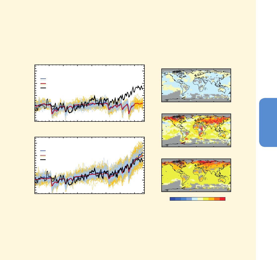
895

Detection and Attribution of Climate Change: from Global to Regional Chapter 10

10.3.2 Water Cycle

Detection and attribution studies of anthropogenic change in hydro-

logic variables are challenged by the length and quality of observed

data sets, and by the difﬁculty in simulating hydrologic variables in

dynamical models. AR4 cautiously noted that the observed increase

in atmospheric water vapour over oceans was consistent with warm-

ing of SSTs attributed to anthropogenic inﬂuence, and that observed

changes in the latitudinal distribution of precipitation, and increased

incidence of drought, were suggestive of a possible human inﬂuence.

Many of the published studies cited in AR4, and some of the studies

FAQ 10.1 (continued)

Overall, FAQ 10.1, Figure 1 shows that the pattern of observed temperature change is signiﬁcantly different than

the pattern of response to natural forcings alone. The simulated response to all forcings, including human-caused

forcings, provides a good match to the observed changes at the surface. We cannot correctly simulate recent

observed climate change without including the response to human-caused forcings, including greenhouse gases,

stratospheric ozone, and aerosols. Natural causes of change are still at work in the climate system, but recent trends

in temperature are largely attributable to human-caused forcing.

FAQ 10.1, Figure 1 | (Left) Time series of global and annual-averaged surface temperature change from 1860 to 2010. The top left panel shows results from two

ensemble of climate models driven with just natural forcings, shown as thin blue and yellow lines; ensemble average temperature changes are thick blue and red lines.

Three different observed estimates are shown as black lines. The lower left panel shows simulations by the same models, but driven with both natural forcing and

human-induced changes in greenhouse gases and aerosols. (Right) Spatial patterns of local surface temperature trends from 1951 to 2010. The upper panel shows the

pattern of trends from a large ensemble of Coupled Model Intercomparison Project Phase 5 (CMIP5) simulations driven with just natural forcings. The bottom panel

shows trends from a corresponding ensemble of simulations driven with natural + human forcings. The middle panel shows the pattern of observed trends from the

Hadley Centre/Climatic Research Unit gridded surface temperature data set 4 (HadCRUT4) during this period.

1860 1880 1900 1920 1940 1960 1980 2000

Year

Temperature anomaly (°C)

Natural and Human forcing

CMIP3

CMIP5

observations

CMIP3

CMIP5

observations

1860 1880 1900 1920 1940 1960 1980 2000

Year

-0.5

0.0

0.5

1.0

1.5

Temperature anomaly (°C)

-0.5

0.0

0.5

1.0

1.5

Natural forcing

180 90W 0 90E 180

90S

45S

45N

90N

Observed trend 1951-2010

180 90W 0 90E 180

90S

45S

45N

90N

Natural and Human forcing

180 90W 0 90E 180

90S

45S

45N

90N

Natural forcing

-2 -1 012

Trend (°C per period)

cited in this section, use less formal detection and attribution criteria

than are often used for assessments of temperature change, owing

to difﬁculties deﬁning large-scale ﬁngerprint patterns of hydrologic

change in models and isolating those ﬁngerprints in data. For example,

correlations between observed hydrologic changes and the patterns of

change in models forced by increasing GHGs can provide suggestive

evidence towards attribution of change.

Since the publication of AR4, in situ hydrologic data sets have been

reanalysed with more stringent quality control. Satellite-derived data

records of worldwide water vapour and precipitation variations have

896

Chapter 10 Detection and Attribution of Climate Change: from Global to Regional

lengthened. Formal detection and attribution studies have been car-

ried out with newer models that potentially offer better simulations

of natural variability. Reviews of detection and attribution of trends in

various components of the water cycle have been published by Stott et

al. (2010) and Trenberth (2011b).

10.3.2.1 Changes in Atmospheric Water Vapour

In situ surface humidity measurements have been reprocessed since

AR4 to create new gridded analyses for climatic research, as discussed

in Chapter 2. The HadCRUH Surface Humidity data set (Willett et

al., 2008) indicates signiﬁcant increases in surface speciﬁc humidity

between 1973 and 2003 averaged over the globe, the tropics, and the

NH, with consistently larger trends in the tropics and in the NH during

summer, and negative or non signiﬁcant trends in relative humidity.

These results are consistent with the hypothesis that the distribution

of relative humidity should remain roughly constant under climate

change (see Section 2.5). Simulations of the response to historical

anthropogenic and natural forcings robustly generate an increase in

atmospheric humidity consistent with observations (Santer et al., 2007;

Willett et al., 2007; Figure 9.9). A recent cessation of the upward trend

in speciﬁc humidity is observed over multiple continental areas in Had-

CRUH and is also found in the European Centre for Medium range

Weather Forecast (ECMWF) interim reanalysis of the global atmos-

phere and surface conditions (ERA-Interim; Simmons et al. 2010). This

change in the speciﬁc humidity trend is temporally correlated with a

levelling off of global ocean temperatures following the 1997–1998 El

Niño event (Simmons et al., 2010).

The anthropogenic water vapour ﬁngerprint simulated by an ensemble

of 22 climate models has been identiﬁed in lower tropospheric mois-

ture content estimates derived from Special Sensor Microwave/Imager

(SSM/I) data covering the period 1988–2006 (Santer et al., 2007).

Santer et al. (2009) ﬁnd that detection of an anthropogenic response

in column water vapour is insensitive to the set of models used. They

rank models based on their ability to simulate the observed mean total

column water vapour, and its annual cycle and variability associated

with ENSO. They report no appreciable differences between the ﬁnger-

prints or detection results derived from the best or worst performing

models, and so conclude that attribution of water vapour changes to

anthropogenic forcing is not sensitive to the choice of models used for

the assessment.

In summary, an anthropogenic contribution to increases in speciﬁc

humidity at and near the Earth’s surface is found with medium con-

ﬁdence. Evidence of a recent levelling off of the long-term surface

atmospheric moistening trend over land needs to be better understood

and simulated as a prerequisite to increased conﬁdence in attribution

studies of water vapour changes. Length and quality of observation-

al humidity data sets, especially above the surface, continue to limit

detection and attribution studies of atmospheric water vapour.

10.3.2.2 Changes in Precipitation

Analysis of CMIP5 model simulations yields clear global and region-

al scale changes associated with anthropogenic forcing (e.g., Scheff

and Frierson, 2012a, 2012b), with patterns broadly similar to those

identiﬁed from CMIP3 models (e.g., Polson et al., 2013). The AR4 con-

cluded that ‘the latitudinal pattern of change in land precipitation and

observed increases in heavy precipitation over the 20th century appear

to be consistent with the anticipated response to anthropogenic forc-

ing’. Detection and attribution of regional precipitation changes gen-

erally focuses on continental areas using in situ data because observa-

tional coverage over oceans is limited to a few island stations (Arkin

et al., 2010; Liu et al., 2012; Noake et al., 2012) , although model-data

comparisons over continents also illustrate large observational uncer-

tainties (Tapiador, 2010; Noake et al., 2012; Balan Sarojini et al., 2012;

Polson et al., 2013). Available satellite data sets that could supplement

oceanic studies are short and their long-term homogeneity is still

unclear (Chapter 2); hence they have not yet been used for detection

and attribution of changes. Continuing uncertainties in climate model

simulations of precipitation make quantitative model/data compari-

sons difﬁcult (e.g., Stephens et al., 2010), which also limits conﬁdence

in detection and attribution. Furthermore, sparse observational cover-

age of precipitation across much of the planet makes the ﬁngerprint

of precipitation change challenging to isolate in observational records

(Balan Sarojini et al., 2012; Wan et al., 2013).

Considering just land regions with sufﬁcient observations, the largest

signal of differences between models with and without anthropogenic

forcings is in the high latitudes of the NH, where increases in precip-

itation are a robust feature of climate model simulations (Scheff and

Frierson, 2012a, 2012b). Such increases have been observed (Figure

10.10) in several different observational data sets (Min et al., 2008a;

Noake et al., 2012; Polson et al., 2013), although high-latitude trends

vary between data sets and with coverage (e.g., Polson et al., 2013).

Attribution of zonally averaged precipitation trends has been attempt-

ed using different observational products and ensembles of forced

simulations from both the CMIP3 and CMIP5 archives, for annu-

al-averaged (Zhang et al., 2007; Min et al., 2008a) and season-spe-

ciﬁc (Noake et al., 2012; Polson et al., 2013) results (Figure 10.11).

Zhang et al. (2007) identify the ﬁngerprint of anthropogenic chang-

es in observed annual zonal mean precipitation averaged over the

periods 1925–1999 and 1950–1999, and separate the anthropogenic

ﬁngerprint from the inﬂuence of natural forcing. The ﬁngerprint of

external forcing is also detected in seasonal means for boreal spring

in all data sets assessed by Noake et al. (2012), and in all but one

data set assessed by Polson et al. (2013) (Figure 10.11), and in boreal

winter in all but one data set (Noake et al., 2012), over the period

1951–1999 and to 2005. The ﬁngerprint features increasing high-lati-

tude precipitation, and decreasing precipitation trends in parts of the

tropics that are reasonably robustly observed in all four data sets con-

sidered albeit with large observational uncertainties north of 60°N

(Figure 10.11). Detection of seasonal-average precipitation change is

less convincing for June, July, August (JJA) and September, October,

November (SON) and results vary with observation data set (Noake

et al., 2012; Polson et al., 2013). Although Zhang et al. (2007) detect

anthropogenic changes even if a separate ﬁngerprint for natural forc-

ings is considered, Polson et al. (2013) ﬁnd that this result is sensi-

tive to the data set used and that the ﬁngerprints can be separated

robustly only for the data set most closely constrained by station data.

The analysis also ﬁnds that model simulated precipitation variability

is smaller than observed variability in the tropics (Zhang et al., 2007;

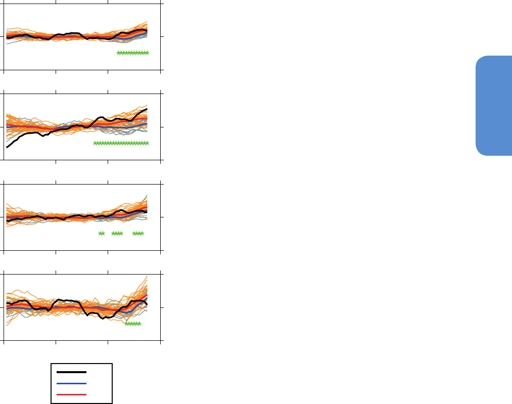
897

Detection and Attribution of Climate Change: from Global to Regional Chapter 10

1950 1970 1990 2010

-0.25

0.00

0.25

Global

0.00

1950 1970 1990 2010

-0.25

0.25

60N-90N

1950 1970 1990 2010

-0.25

0.00

0.25

30N-60N

Land masked by Obs

1950 1970 1990 2010

-0.25

0.00

0.25

30S-30N

All

Nat

Obs

Figure 10.10 | Global and zonal average changes in annual mean precipitation (mm

day

–1

) over areas of land where there are observations, expressed relative to the base-

line period of 1961–1990, simulated by CMIP5 models forced with both anthropogenic

and natural forcings (red lines) and natural forcings only (blue lines) for the global mean

and for three latitude bands. Multi-model means are shown in thick solid lines. Observa-

tions (gridded values derived from Global Historical Climatology Network station data,

updated from Zhang et al. (2007) are shown as a black solid line. An 11-year smoothing

is applied to both simulations and observations. Green stars show statistically signiﬁcant

changes at 5% level (p value <0.05) between the ensemble of runs with both anthropo-

genic and natural forcings (red lines) and the ensemble of runs with just natural forcings

(blue lines) using a two-sample two-tailed t-test for the last 30 years of the time series.

(From Balan Sarojini et al., 2012.) Results for the Climate Research Unit (CRU) TS3.1

data set are shown in Figure 10.A.2.

Polson et al., 2013) which is addressed by increasing the estimate of

variance from models (Figure 10.11).

Another detection and attribution study focussed on precipitation in

the NH high latitudes and found an attributable human inﬂuence (Min

et al., 2008a). Both Min et al. (2008a) and Zhang et al. (2007) ﬁnd that

the observed changes are signiﬁcantly larger than the model simulated

changes. However, Noake et al. (2012) and Polson et al. (2013) ﬁnd that

the difference between models and observations decreases if changes

are expressed as a percentage of climatological precipitation and that

the observed and simulated changes are largely consistent between

CMIP5 models and observations given data uncertainty. Use of addi-

tional data sets illustrates remaining observational uncertainty in high

latitudes of the NH (Figure 10.11). Regional-scale attribution of pre-

cipitation change is still problematic although regional climate models

have yielded simulations consistent with observed wintertime changes

for northern Europe (Bhend and von Storch, 2008; Tapiador, 2010).

Precipitation change over ocean has been attributed to human inﬂu-

ence by Fyfe et al. (2012) for the high-latitude SH in austral summer,

where zonally averaged precipitation has declined around 45°S and

increased around 60°S since 1957, consistent with CMIP5 historical

simulations, with the magnitude of the half-century trend outside the

range of simulated natural variability. Conﬁdence in this attribution

result, despite limitations in precipitation observations, is enhanced by

its consistency with trends in large-scale sea level pressure data (see

Section 10.3.3).

In summary, there is medium conﬁdence that human inﬂuence has con-

tributed to large-scale changes in precipitation patterns over land. The

expected anthropogenic ﬁngerprints of change in zonal mean precip-

itation—reductions in low latitudes and increases in NH mid to high

latitudes—have been detected in annual and some seasonal data.

Observational uncertainties including limited global coverage and large

natural variability, in addition to challenges in precipitation modeling,

limit conﬁdence in assessment of climatic changes in precipitation.

10.3.2.3 Changes in Surface Hydrologic Variables

This subsection assesses recent research on detection and attribu-

tion of long-term changes in continental surface hydrologic variables,

including soil moisture, evapotranspiration and streamﬂow. Stream-

ﬂows are often subject to large non-climatic human inﬂuence, such as

diversions and land use changes, that must be accounted for in order

to attribute detected hydrologic changes to climate change. Cryospher-

ic aspects of surface hydrology are discussed in Section 10.5; extremes

in surface hydrology (such as drought) and precipitation are covered in

Section 10.6.1. The variables discussed here are subject to large mod-

eling uncertainties (Chapter 9) and observational challenges (Chapter

2), which in combination place severe limits on climate change detec-

tion and attribution.

Direct observational records of soil moisture and surface ﬂuxes tend

to be sparse and/or short, thus limiting recent assessments of change

in these variables (Jung et al., 2010). Assimilated land surface data

sets and new satellite observations (Chapter 2) are promising tools,

but assessment of past and future climate change of these variables

(Hoekema and Sridhar, 2011) is still generally carried out on derived

quantities such as the Palmer Drought Severity Index, as discussed

more fully in Section 10.6.1. Recent observations (Jung et al., 2010)

show regional trends towards drier soils. An optimal detection analysis

of reconstructed evapotranspiration identiﬁes the effects of anthro-

pogenic forcing on evapotranspiration, with the Centre National de

Recherches Météorologiques (CNRM)-CM5 model simulating chang-

es consistent with those estimated to have occurred (Douville et al.,

2013).

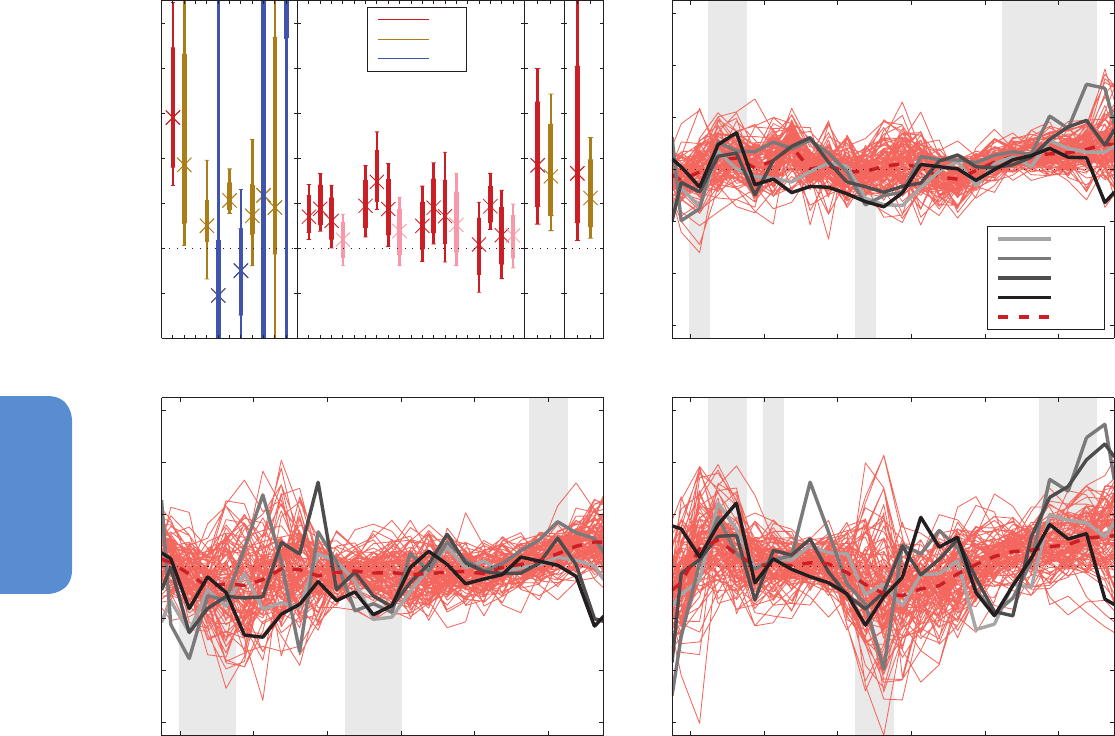
898

Chapter 10 Detection and Attribution of Climate Change: from Global to Regional

−40 −20 0204060

−6

−4

−2

Latitude

Precipitation trend (% per decade)

JJA(f)

−40 −20 0204060

−6

−4

−2

Latitude

Precipitation trend (% per decade)

DJF(g)

−40 −20 0204060

−6

−4

−2

Latitude

Precipitation trend (% per decade)

ANNUAL(e)

Obs(V)

Obs(Z)

Obs(C)

Obs(G)

ZZ C Z V G

−4

−2

Scaling factor

(a)

1−sig 2−sig

CZVG CZVG CZVG CZVG

Observation dataset

(b)

DJF MAM JJA SON

ALL

ANT

NAT

(c)

(d)

Figure 10.11 | Detection and attribution results for zonal land precipitation trends in the second half of the 20th century. (Top left) Scaling factors for precipitation changes. (Top

right and bottom) Zonally averaged precipitation changes over continents from models and observations. (a) Crosses show the best-guess scaling factor derived from multi-model

means. Thick bars show the 5 to 95% uncertainty range derived from model-simulated variability, and thin bars show the uncertainty range if doubling the multi-model variance.

Red bars indicate scaling factors for the estimated response to all forcings, blue bars for natural-only forcing and brown bars for anthropogenic-only forcing. Labels on the x-axis

identify results from four different observational data sets (Z is Zhang et al. (2007), C is Climate Research Unit (CRU), V is Variability Analyses of Surface Climate Observations (Vas-

ClimO), G is Global Precipitation Climatology Centre (GPCC), H is Hadley Centre gridded data set of temperature and precipitation extremes (HadEX)). (a) Detection and attribution

results for annual averages, both single ﬁngerprint (“1-sig”; 1950–1999) and two ﬁngerprint results (“2-sig”; Z, C, G (1951–2005), V (1952–2000)). (b) Scaling factors resulting

from single-ﬁngerprint analyses for seasonally averaged precipitation (Z, C, G (1951–2005), V (1952–2000); the latter in pink as not designed for long-term homogeneity) for four

different seasons. (c) Scaling factors for spatial pattern of Arctic precipitation trends (1951–1999). (d) Scaling factors for changes in large-scale intense precipitation (1951–1999).

(e) Thick solid lines show observed zonally and annually averaged trends (% per decade) for four different observed data sets. Corresponding results from individual simulations

from 33 different climate models are shown as thin solid lines, with the multimodel mean shown as a red dashed line. Model results are masked to match the spatial and temporal

coverage of the GPCC data set (denoted G in the seasonal scaling factor panel). Grey shading indicates latitude bands within which >75% of simulations yield positive or negative

trends. (f, g) Like (e) but showing zonally averaged precipitation changes for (f) June, July, August (JJA) and (g) December, January, February (DJF) seasons. Scaling factors (c) and (d)

adapted from Min et al. (2008a) and Min et al. (2011), respectively; other results adapted from Zhang et al. (2007) and Polson et al. (2013).

Trends towards earlier timing of snowmelt-driven streamﬂows in west-

ern North America since 1950 have been demonstrated to be differ-

ent from natural variability (Hidalgo et al., 2009). Similarly, internal

variability associated with natural decade-scale ﬂuctuations could

not account for recent observed declines of northern Rocky Mountain

streamﬂow (St Jacques et al., 2010). Statistical analyses of stream-

ﬂows demonstrate regionally varying changes that are consistent with

changes expected from increasing temperature, in Scandinavia (Wilson

et al., 2010), Europe (Stahl et al., 2010) and the USA (Krakauer and

Fung, 2008; Wang and Hejazi, 2011). Observed increases in Arctic river

discharge, which could be a good integrator for monitoring changes

in precipitation in high latitudes, are found to be explainable only if

model simulations include anthropogenic forcings (Min et al., 2008a).

Barnett et al. (2008) analysed changes in the surface hydrology of

the western USA, considering snow pack (measured as snow water

equivalent), the seasonal timing of streamﬂow in major rivers, and

average January to March daily minimum temperature over the region,

the two hydrological variables they studied being closely related to

temperature. Observed changes were compared with the output of a

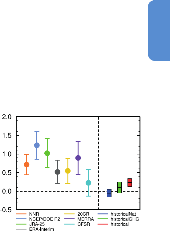
899

Detection and Attribution of Climate Change: from Global to Regional Chapter 10

regional hydrologic model forced by the Parallel Climate Model (PCM)

and Model for Interdisciplinary Research On Climate (MIROC) climate

models. They derived a ﬁngerprint of anthropogenic changes from the

two climate models and found that the observations, when projected

onto the ﬁngerprint of anthropogenic changes, show a positive signal

strength consistent with the model simulations that falls outside

the range expected from internal variability as estimated from 1600

years of downscaled climate model data. They conclude that there is a

detectable and attributable anthropogenic signature on the hydrology

of this region.

In summary, there is medium conﬁdence that human inﬂuence on

climate has affected stream ﬂow and evapotranspiration in limited

regions of middle and high latitudes of the NH. Detection and attribu-

tion studies have been applied only to limited regions and using a few

models. Observational uncertainties are large and in the case of evap-

otranspiration depend on reconstructions using land surface models.

10.3.3 Atmospheric Circulation and Patterns of Variability

The atmospheric circulation is driven by various processes including

the uneven heating of the Earth’s surface by solar radiation, land–sea

contrast and orography. The circulation transports heat from warm to

cold regions and thereby acts to reduce temperature contrasts. Thus,

changes in circulation and in patterns of variability are of critical impor-

tance for the climate system, inﬂuencing regional climate and regional

climate variability. Any such changes are important for local climate

change because they could act to reinforce or counteract the effects of

external forcings on climate in a particular region. Observed changes

in atmospheric circulation and patterns of variability are assessed in

Section 2.7.5. Although new and improved data sets are now available,

changes in patterns of variability remain difﬁcult to detect because of

large variability on interannual to decadal time scales (Section 2.7).

Since AR4, progress has been made in understanding the causes of

changes in circulation-related climate phenomena and modes of var-

iability such as the width of the tropical circulation, and the Southern

Annular Mode (SAM). For other climate phenomena, such as ENSO,

Indian Ocean Dipole (IOD), Paciﬁc Decadal Oscillation (PDO), and mon-

soons, there are large observational and modelling uncertainties (see

Section 9.5 and Chapter 14), and there is low conﬁdence that changes

in these phenomena, if observed, can be attributed to human-induced

inﬂuence.

10.3.3.1 Tropical Circulation

Various indicators of the width of the tropical belt based on independ-

ent data sets suggest that the tropical belt as a whole has widened

since 1979; however, the magnitude of this change is very uncertain

(Fu et al., 2006; Hudson et al., 2006; Hu and Fu, 2007; Seidel and

Randel, 2007; Seidel et al., 2008; Lu et al., 2009; Fu and Lin, 2011;

Hu et al., 2011; Davis and Rosenlof, 2012; Lucas et al., 2012; Wilcox

et al., 2012; Nguyen et al., 2013) (Section 2.7.5). CMIP3 and CMIP5

simulations suggest that anthropogenic forcings have contributed to

the observed widening of the tropical belt since 1979 (Johanson and

Fu, 2009; Hu et al., 2013). On average the poleward expansion of the

Hadley circulation and other indicators of the width of the tropical belt

is greater than determined from CMIP3 and CMIP5 simulations (Seidel

et al., 2008; Johanson and Fu, 2009; Hu et al., 2013; Figure 10.12). The

causes as to why models underestimate the observed poleward expan-

sion of the tropical belt are not fully understood. Potential factors are

lack of understanding of the magnitude of natural variability as well

as changes in observing systems that also affect reanalysis products

(Thorne and Vose, 2010; Lucas et al., 2012; Box 2.3).

Climate model simulations suggest that Antarctic ozone depletion is

a major factor in causing poleward expansion of the southern Hadley

cell during austral summer over the last three to ﬁve decades with

GHGs also playing a role (Son et al., 2008, 2009, 2010; McLandress

et al., 2011; Polvani et al., 2011; Hu et al., 2013). In reanalysis data

a detectable signal of ozone forcing is separable from other external

forcing including GHGs when utilizing both CMIP5 and CMIP3 simu-

lations combined (Min and Son, 2013). An analysis of CMIP3 simula-

tions suggests that BC aerosols and tropospheric ozone were the main

drivers of the observed poleward expansion of the northern Hadley

cell in boreal summer (Allen et al., 2012). It is found that global green-

house warming causes increase in static stability, such that the onset

of baroclinicity is shifted poleward, leading to poleward expansion of

the Hadley circulation (Frierson, 2006; Frierson et al., 2007; Hu and

Fu, 2007; Lu et al., 2007, 2008). Tropical SST increase may also con-

tribute to a widening of the Hadley circulation (Hu et al., 2011; Staten

et al., 2012). Althoughe some Atmospheric General Circulation Model

(AGCM) simulations forced by observed time-varying SSTs yield a wid-

ening by about 1° in latitude over 1979–2002 (Hu et al., 2011), other

simulations suggest that SST changes have little effect on the tropical

expansion when based on the tropopause metric of the tropical width

(Lu et al., 2009). However, it is found that the tropopause metric is not

Poleward expansion (°C per decade)

Figure 10.12 | December to February mean change of southern border of the Hadley

circulation. Unit is degree in latitude per decade. Reanalysis data sets (see also Box 2.3)

are marked with different colours. Trends are all calculated over the period of 1979–

2005. The terms historicalNAT, historicalGHG, and historical denote CMIP5 simulations

with natural forcing, with greenhouse gas forcing and with both anthropogenic and

natural forcings, respectively. For each reanalysis data set, the error bars indicate the

95% conﬁdence level of the standard t-test. For CMIP5 simulations, trends are ﬁrst

calculated for each model, and all ensemble members of simulations are used. Then,

trends are averaged for multi-model ensembles. Trend uncertainty is estimated from

multi-model ensembles, as twice the standard error. (Updated from Hu et al., 2013.)

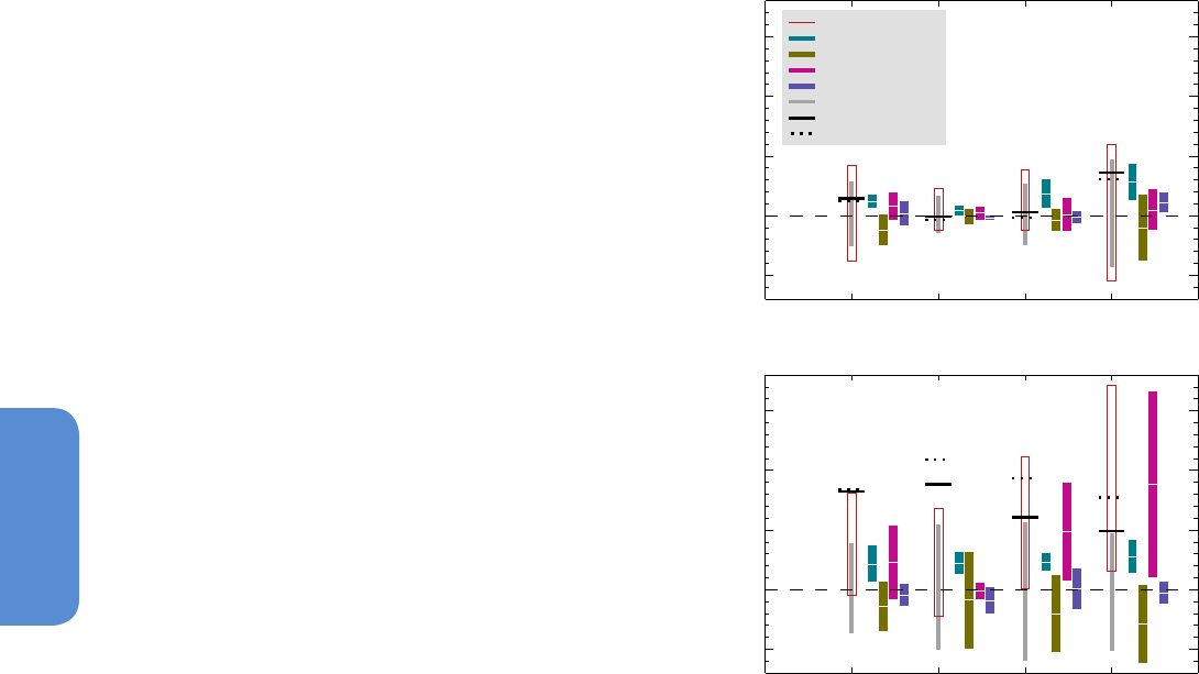
900

Chapter 10 Detection and Attribution of Climate Change: from Global to Regional

very reliable because of the use of arbitrary thresholds (Birner, 2010;

Davis and Rosenlof, 2012).

In summary, there are multiple lines of evidence that the Hadley cell

and the tropical belt as a whole have widened since at least 1979;

however, the magnitude of the widening is very uncertain. Based on

modelling studies there is medium conﬁdence that stratospheric ozone

depletion has contributed to the observed poleward shift of the south-

ern Hadley cell border during austral summer, with GHGs also playing

a role. The contribution of internal climate variability to the observed

poleward expansion of the Hadley circulation remains very uncertain.

10.3.3.2 Northern Annular Mode/North Atlantic Oscillation

The NAO, which exhibited a positive trend from the 1960s to the 1990s,

has since exhibited lower values, with exceptionally low anomalies in

the winters of 2009/2010 and 2010/2011 (Section 2.7.8). This means

that the positive trend in the NAO discussed in the AR4 has considera-

bly weakened when evaluated up to 2011. Similar results apply to the

closely related Northern Annular Mode (NAM), with its upward trend

over the past 60 years in the 20th Century Reanalysis (Compo et al.,

2011) and in Hadley Centre Sea Level Pressure data set 2r (HadSLP2r;

Allan and Ansell, 2006) not being signiﬁcant compared to internal var-

iability (Figure 10.13). An analysis of CMIP5 models shows that they

simulate positive trends in NAM in the DJF season over this period,

albeit not as large as those observed which are still within the range of

natural internal variability (Figure 10.13).

Other work (Woollings, 2008) demonstrates that while the NAM is

largely barotropic in structure, the simulated response to anthropogen-

ic forcing has a strong baroclinic component, with an opposite geopo-

tential height trends in the mid-troposphere compared to the surface

in many models. Thus while the circulation response to anthropogenic

forcing may project onto the NAM, it is not entirely captured by the

NAM index.

Consistent with previous ﬁndings (Hegerl et al., 2007b), Gillett and

Fyfe (2013) ﬁnd that GHGs tend to drive a positive NAM response in

the CMIP5 models. Recent modelling work also indicates that ozone

changes drive a small positive NAM response in spring (Morgenstern

et al., 2010; Gillett and Fyfe, 2013).

10.3.3.3 Southern Annular Mode

The Southern Annular Mode (SAM) index has remained mainly positive

since the publication of the AR4, although it has not been as strongly

positive as in the late 1990s. Nonetheless, an index of the SAM shows

a signiﬁcant positive trend in most seasons and data sets over the

1951–2011 period (Figure 10.13; Table 2.14). Recent modelling studies

conﬁrm earlier ﬁndings that the increase in GHG concentrations tends

to lead to a strengthening and poleward shift of the SH eddy-driven

polar jet (Karpechko et al., 2008; Son et al., 2008, 2010; Sigmond et al.,

2011; Staten et al., 2012; Swart and Fyfe, 2012; Eyring et al., 2013; Gil-

lett and Fyfe, 2013) which projects onto the positive phase of the SAM.

Stratospheric ozone depletion also induces a strengthening and pole-

ward shift of the polar jet in models, with the largest response in aus-

tral summer (Karpechko et al., 2008; Son et al., 2008, 2010; McLandress

MAM JJA SON DJF

Season

-0.5

0.0

0.5

1.0

1.5

SAM trend (hPa per decade)

MAM JJA SON DJF

Season

-0.5

0.0

0.5

1.0

1.5

NAM trend (hPa per decade)

historical

historicalGHG

historicalAer

historicalOz

historicalNat

control

HadSLP2

20CR

(a)

(b)

Figure 10.13 | Simulated and observed 1951–2011 trends in the Northern Annular

Mode (NAM) index (a) and Southern Annular Mode (SAM) index (b) by season. The NAM

is a Li and Wang (2003) index based on the difference between zonal mean seal level

pressure (SLP) at 35°N and 65°N. and the, and the SAM index is a difference between

zonal mean SLP at 40°S and 65°S (Gong and Wang, 1999). Both indices are deﬁned

without normalization, so that the magnitudes of simulated and observed trends can

be compared. Black lines show observed trends from the HadSLP2r data set (Allan and

Ansell, 2006) (solid), and the 20th Century Reanalysis (Compo et al., 2011) (dotted).

Grey bars and red boxes show 5 to 95% ranges of trends in CMIP5 control and histori-

cal simulations respectively. Ensemble mean trends and their 5 to 95% uncertainties

are shown for the response to greenhouse gases (light green), aerosols (dark green),

ozone (magenta) and natural (blue) forcing changes, based on CMIP5 individual forcing

simulations. (Adapted from Gillett and Fyfe, 2013.)

et al., 2011; Polvani et al., 2011; Sigmond et al., 2011; Gillett and Fyfe,

2013). Sigmond et al. (2011) ﬁnd approximately equal contributions

to simulated annual mean SAM trends from GHGs and stratospher-

ic ozone depletion up to the present. Fogt et al. (2009) demonstrate

that observed SAM trends over the period 1957–2005 are positive in

all seasons, but only statistically signiﬁcant in DJF and March, April,

May (MAM), based on simulated internal variability. Roscoe and Haigh

(2007) apply a regression-based approach and ﬁnd that stratospheric

ozone changes are the primary driver of observed trends in the SAM.

Observed trends are also consistent with CMIP3 simulations including

stratospheric ozone changes in all seasons, though in MAM observed

trends are roughly twice as large as those simulated (Miller et al., 2006).

Broadly consistent results are found when comparing observed trends

and CMIP5 simulations (Figure 10.13), with a station-based SAM index

showing a signiﬁcant positive trend in MAM, JJA and DJF, compared

901

Detection and Attribution of Climate Change: from Global to Regional Chapter 10

to simulated internal variability over the 1951–2010 period. Fogt et

al. (2009) ﬁnd that the largest forced response has likely occurred in

DJF, the season in which stratospheric ozone depletion has been the

dominant contributor to the observed trends.

Taking these ﬁndings together, it is likely that the positive trend in

the SAM seen in austral summer since the mid-20th century is due in

part to stratospheric ozone depletion. There is medium conﬁdence that

GHGs have also played a role.

10.3.3.4 Change in Global Sea Level Pressure Patterns

A number of studies have applied formal detection and attribution

studies to global ﬁelds of atmospheric SLP ﬁnding detection of human

inﬂuence on global patterns of SLP (Gillett et al., 2003, 2005; Gil-

lett and Stott, 2009). Analysing the contributions of different forcings

to observed changes in SLP, Gillett and Stott (2009) ﬁnd separately

detectable inﬂuences of anthropogenic and natural forcings in zonal

mean seasonal mean SLP, strengthening evidence for a human inﬂu-

ence on SLP. Based on the robustness of the evidence from multiple

models we conclude that it is likely that human inﬂuence has altered

SLP patterns globally since 1951.

10.4 Changes in Ocean Properties

This section assesses the causes of oceanic changes in the main prop-

erties of interest for climate change: ocean heat content, ocean salinity

and freshwater ﬂuxes, sea level, oxygen and ocean acidiﬁcation.

10.4.1 Ocean Temperature and Heat Content

The oceans are a key part of the Earth’s energy balance (Boxes 3.1 and

13.1). Observational studies continue to demonstrate that the ocean

heat content has increased in the upper layers of the ocean during

the second half of the 20th century and early 21st century (Section

3.2; Bindoff et al., 2007), and that this increase is consistent with a

net positive radiative imbalance in the climate system. It is of signiﬁ-

cance that this heat content increase is an order of magnitude larger

than the increase in energy content of any other component of the

Earth’s ocean–atmosphere–cryosphere system and accounts for more

than 90% of the Earth’s energy increase between 1971 and 2010 (e.g.,

Boxes 3.1 and 13.1; Bindoff et al., 2007; Church et al., 2011; Hansen

et al., 2011).

Despite the evidence for anthropogenic warming of the ocean, the

level of conﬁdence in the conclusions of the AR4 report—that the

warming of the upper several hundred meters of the ocean during the

second half of the 20th century was likely to be due to anthropogenic

forcing—reﬂected the level of uncertainties at that time. The major

uncertainty was an apparently large decadal variability (warming in

the 1970s and cooling in the early 1980s) in the observational esti-

mates that was not simulated by climate models (Hegerl et al., 2007b,

see their Table 9.4). The large decadal variability in observations raised

concerns about the capacity of climate models to simulate observed

variability. There were also lingering concerns about the presence of

non-climate–related biases in the observations of ocean heat content

change (Gregory et al., 2004; AchutaRao et al., 2006). After the IPCC

AR4 report in 2007, time-and depth-dependent systematic errors in

bathythermograph temperatures were discovered (Gouretski and

Koltermann, 2007; Section 3.2). Bathythermograph data account for a

large fraction of the historical temperature observations and are there-

fore a source of bias in ocean heat content studies. Bias corrections

were then developed and applied to observations. With the newer

bias-corrected estimates (Domingues et al., 2008; Wijffels et al., 2008;

Ishii and Kimoto, 2009; Levitus et al., 2009), it became obvious that the

large decadal variability in earlier estimates of global upper-ocean heat

content was an observational artefact (Section 3.2).

The interannual to decadal variability of ocean temperature simulat-

ed by the CMIP3 models agrees better with observations when the

model data is sampled using the observational data mask (AchutaRao

et al., 2007). In the upper 700 m, CMIP3 model simulations agreed

more closely with observational estimates of global ocean heat con-

tent based on bias-corrected ocean temperature data, both in terms of

the decadal variability and multi-decadal trend (Figure 10.14a) when

forced with the most complete set of natural and anthropogenic forc-

ings (Domingues et al., 2008). For the simulations with the most com-

plete set of forcings, the multi-model ensemble mean trend was only

10% smaller than observed for 1961–1999. Model simulations that

included only anthropogenic forcing (i.e., no solar or volcanic forcing)

signiﬁcantly overestimate the multi-decadal trend and underestimate

decadal variability. This overestimate of the trend is partially caused

by the ocean’s response to volcanic eruptions, which results in rapid

cooling followed by decadal or longer time variations during the recov-

ery phase. Although it has been suggested (Gregory, 2010) that the

cooling trend from successive volcanic events is an artefact because

models were not spun up with volcanic forcing, this discrepancy is not

expected to be as signiﬁcant in the upper ocean as in the deeper layers

where longer term adjustments take place (Gregory et al., 2012 ). Thus

for the upper ocean, there is high conﬁdence that the more frequent

eruptions during the second half of the 20th century have caused a

multi-decadal cooling that partially offsets the anthropogenic warm-

ing and contributes to the apparent decadal variability (Church et al.,

2005; Delworth et al., 2005; Fyfe, 2006; Gleckler et al., 2006; Gregory

et al., 2006; AchutaRao et al., 2007; Domingues et al., 2008; Palmer et

al., 2009; Stenchikov et al., 2009).

Gleckler et al. (2012) examined the detection and attribution of upper-

ocean warming in the context of uncertainties in the underlying

observational data sets, models and methods. Using three bias-cor-

rected observational estimates of upper-ocean temperature changes

(Domingues et al., 2008; Ishii and Kimoto, 2009; Levitus et al., 2009)

and models from the CMIP3 multi-model archive, they found that mul-

ti-decadal trends in the observations were best understood by includ-

ing contributions from both natural and anthropogenic forcings. The

anthropogenic ﬁngerprint in observed upper-ocean warming, driven by

global mean and basin-scale pattern changes, was also detected. The

strength of this signal (estimated from successively longer trend peri-

ods of ocean heat content starting from 1970) crossed the 5% and 1%

signiﬁcance threshold in 1980 and progressively becomes more strong-

ly detected for longer trend periods (Figure 10.14b), for all ocean heat

content time series. This stronger detection for longer periods occurs

because the noise (standard deviation of trends in the unforced chang-

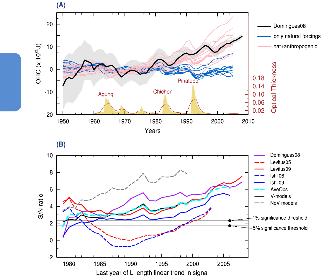
902

Chapter 10 Detection and Attribution of Climate Change: from Global to Regional

es in pattern similarity from model control runs) tends to decrease for

longer trend lengths. On decadal time scales, there is limited evidence

that basin scale space-time variability structure of CMIP3 models is

approximately 25% lower than the (poorly constrained) observations,

this underestimate is far less than the factor of 2 needed to throw

the anthropogenic ﬁngerprint into question. This result is robust to a

number of known observational, model, methodological and structural

uncertainties.

An analysis of upper-ocean (0 to 700 m) temperature changes for

1955–2004, using bias-corrected observations and 20 global climate

models from CMIP5 (Pierce et al., 2012) builds on previous detection

and attribution studies of ocean temperature (Barnett et al., 2001,

2005; Pierce et al., 2006). This analysis found that observed tempera-

ture changes during the above period are inconsistent with the effects

of natural climate variability. That is signal strengths are separated

from zero at the 5% signiﬁcance level, and the probability that the

Figure 10.14 | (A) Comparison of observed global ocean heat content for the upper 700 m (updated from Domingues et al. 2008) with simulations from ten CMIP5 models that

included only natural forcings (‘HistoricalNat’ runs shown in blue lines) and simulations that included natural and anthropogenic forcings (‘Historical’ runs in pink lines). Grey shad-

ing shows observational uncertainty. The global mean stratospheric optical depth (Sato et al., 1993) in beige at the bottom indicates the major volcanic eruptions and the brown

curve is a 3-year running average of these values. (B) Signal-to-noise (S/N) ratio (plotted as a function of increasing trend length L) of basin-scale changes in volume averaged

temperature of newer, expendable bathythermograph (XBT)-corrected data (solid red, purple and blue lines), older, uncorrected data (dashed red and blue lines); the average of

the three corrected observational sets (AveObs; dashed cyan line); and simulations that include volcanic (V) or exclude volcanic eruptions (NoV) (black solid and grey dashed lines

respectively). The start date for the calculation of signal trends is 1970 and the initial trend length is 10 years. The 1% and 5% signiﬁcance thresholds are shown (as horizontal grey

lines) and assume a Gaussian distribution of noise trends in the V-models control-run pseudo-principal components. The detection time is deﬁned as the year at which S/N exceeds

and remains above 1% or 5% signiﬁcance threshold (Gleckler et al., 2012).

903

Detection and Attribution of Climate Change: from Global to Regional Chapter 10

null hypothesis of observed changes being consistent with natural var-

iability is less than 0.05 from variability either internal to the climate

system alone, or externally forced by solar ﬂuctuations and volcanic

eruptions. However, the observed ocean changes are consistent with

those expected from anthropogenically induced atmospheric changes

from GHGs and aerosol concentrations.

Attribution to anthropogenic warming from recent detection and attri-

bution studies (Gleckler et al., 2012; Pierce et al., 2012) have made use

of new bias-corrected observations and have systematically explored

methodological uncertainties, yielding more conﬁdence in the results.

With greater consistency and agreement across observational data

sets and resolution of structural issues, the major uncertainties at the

time of AR4 have now largely been resolved. The high levels of conﬁ-

dence and the increased understanding of the contributions from both

natural and anthropogenic sources across the many studies mean that

it is very likely that the increase in global ocean heat content observed

in the upper 700 m since the 1970s has a substantial contribution from

anthropogenic forcing.

Although there is high conﬁdence in understanding the causes of global

heat content increases, attribution of regional heat content changes

are less certain. Earlier regional studies used a ﬁxed depth data and

only considered basin-scale averages (Barnett et al., 2005). At regional

scales, however, changes in advection of ocean heat are important and

need to be isolated from changes due to air–sea heat ﬂuxes (Palmer

et al., 2009; Grist et al., 2010). Their ﬁxed isotherm (rather than ﬁxed

depth) approach to optimal detection analysis, in addition to being

largely insensitive to observational biases, is designed to separate the

ocean’s response to air–sea ﬂux changes from advective changes. Air–

sea ﬂuxes are the primary mechanism by which the oceans are expect-

ed to respond to externally forced anthropogenic and natural volcanic

inﬂuences. The ﬁner temporal resolution of the analysis allowed Palmer

et al. (2009) to attribute distinct short-lived cooling episodes to major

volcanic eruptions while, at multi-decadal time scales, a more spatially

uniform near-surface (~ upper 200 m) warming pattern was detected

across all ocean basins (except in high latitudes where the isotherm

approach has limitations due to outcropping of isotherms at the ocean

surface) and attributed to anthropogenic causes at the 5% signiﬁcance

level. Considering that individual ocean basins are affected by different

observational and modelling uncertainties and that internal variabili-

ty is larger at smaller scales, detection of signiﬁcant anthropogenic

forcing through space and time studies (Palmer et al., 2009; Pierce et

al., 2012) provides more compelling evidence of human inﬂuence at

regional scales of near-surface ocean warming observed during the

second half of the 20th century.

10.4.2 Ocean Salinity and Freshwater Fluxes

There is increasing recognition of the importance of ocean salinity as

an essential climate variable (Doherty et al., 2009), particularly for

understanding the hydrological cycle. In the IPCC Fourth Assessment

Report observed ocean salinity change indicated that there was a sys-

tematic pattern of increased salinity in the shallow subtropics and a

tendency to freshening of waters that originate in the polar regions

(Bindoff et al., 2007; Hegerl et al., 2007b) (Figure 10.15a, upper and

lower panels). New atlases and revisions of the earlier work based on

the increasing number of the Array for Real-time Geostrophic Ocean-

ography (ARGO) proﬁle data, and historical data have extended the

observational salinity data sets allowing the examination of the long-

term changes at the surface and in the interior of the ocean (Section

3.3) and supporting analyses of precipitation changes over land (see

Sections 10.3.2.2 and 2.5.1).

Patterns of subsurface salinity changes largely follow the existing

mean salinity pattern at the surface and within the ocean. For example,

the inter-basin contrast between the Atlantic (salty) and Paciﬁc Oceans

(fresh) has intensiﬁed over the observed record (Boyer et al., 2005;

Hosoda et al., 2009; Roemmich and Gilson, 2009; von Schuckmann

et al., 2009; Durack and Wijffels, 2010). In the Southern Ocean, many

studies show a coherent freshening of Antarctic Intermediate Water

that is subducted at about 50°S (Johnson and Orsi, 1997; Wong et al.,

1999; Bindoff and McDougall, 2000; Curry et al., 2003; Boyer et al.,

2005; Roemmich and Gilson, 2009; Durack and Wijffels, 2010; Helm et

al., 2010; Kobayashi et al., 2012). There is also a clear increase in salin-

ity of the high-salinity subtropical waters (Durack and Wijffels, 2010;

Helm et al., 2010).

The 50-year trends in surface salinity show that there is a strong pos-

itive correlation between the mean climate of the surface salinity and

its temporal changes from 1950 to 2000 (see Figures 3.4 and 10.15b

‘ocean obs’ point). The correlation between the climate and the trends

in surface salinity of 0.7 implies that fresh surface waters get fresh-

er, and salty waters get saltier (Durack et al., 2012). Such patterns of

surface salinity change are also found in Atmosphere–Ocean General

Circulation Models (AOGCM) simulations both for the 20th century

and projected future changes into the 21st century (Figure 10.15b).

The pattern of temporal change in observations from CMIP3 simula-

tions is particularly strong for those projections using Special Report on

Emission Scenarios (SRES) with larger global warming changes (Figure

10.15b). For the period 1950–2000 the observed ampliﬁcation of the

surface salinity is 16 ± 10% per °C of warming and is twice the simu-

lated surface salinity change in CMIP3 models. This difference between

the surface salinity ampliﬁcation is plausibly caused by the tendency

of CMIP3 ocean models mixing surface salinity into deeper layers and

consequently surface salinity increases at a slower rate than observed

(Durack et al., 2012).

Although there are now many established observed long-term trends

of salinity change at the ocean surface and within the interior ocean

at regional and global scales (Section 3.3), there are relatively few

studies that attribute these changes formally to anthropogenic forcing.

Analysis at the regional scale of the observed recent surface salinity

increases in the North Atlantic (20°N to 50°N) show a small signal that

could be attributed to anthropogenic forcings but for this ocean is not

signiﬁcant compared with internal variability (Stott et al., 2008a; Terray

et al., 2012; and Figure 10.15c). On a larger spatial scale, the surface

salinity patterns in the band from 30°S to 50°N show anthropogenic

contributions that are larger than the 5 to 95% uncertainty range

(Terray et al., 2012). The strongest signals that can be attributed to

anthropogenic forcing are in the tropics (TRO, 30°S to 30°N) and the

western Paciﬁc. These results also show the salinity contrast between

the Paciﬁc and Atlantic oceans is also enhanced with signiﬁcant

contributions from anthropogenic forcing.

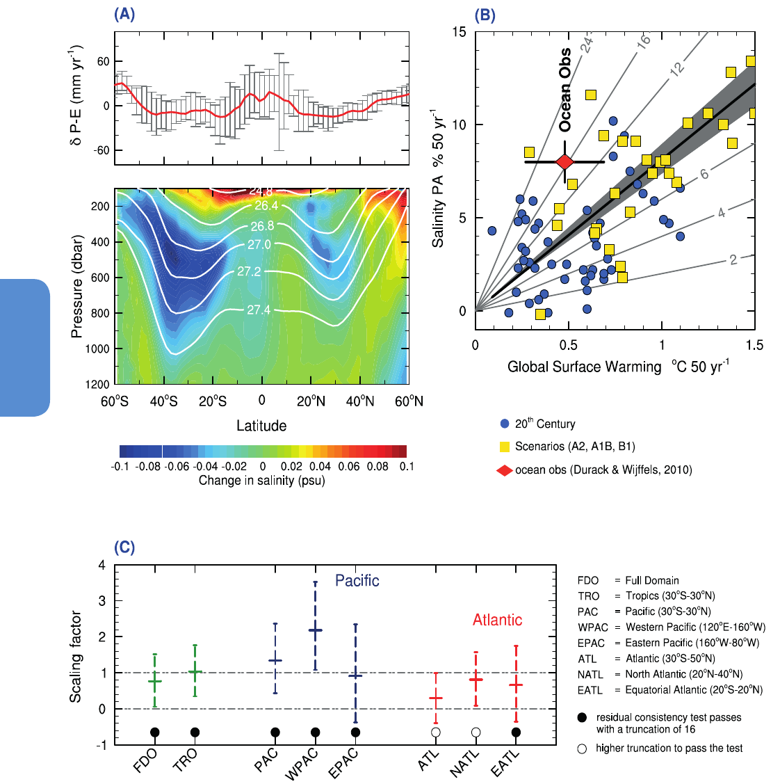
904

Chapter 10 Detection and Attribution of Climate Change: from Global to Regional

(

)

(

)

Figure 10.15 | Ocean salinity change and hydrologic cycle. (A) Ocean salinity change observed in the interior of the ocean (A, lower panel in practical salinity units or psu, and

white lines are surfaces of constant density) and comparison with ten CMIP3 model projections of precipitation minus evaporation δ (P – E) in mm yr

–1

for the same period as the

observed changes (1970 to 1990s) (A, top panel, red line is the mean of the simulations and error bars are the simulated range). (B) The ampliﬁcation of the current surface salinity

pattern over a 50-year period as a function of global temperature change. Ocean surface salinity pattern ampliﬁcation has a 16% increase for the 1950–2000 period (red diamond,

see text and Section 3.3). Also on this panel CMIP3 simulations from Special Report on Emission Scenarios (SRES) (yellow squares) and from 20th century simulations (blue circles).

A total of 93 simulations have been used. (C) Regional detection and attribution in the equatorial Paciﬁc and Atlantic Oceans for 1970 to 2002. Scaling factors for all forcings

(anthropogenic) ﬁngerprint are shown (see Box 10.1) with their 5 to 95% uncertainty range, estimated using the total least square approach. Full domain (FDO, 30°S to 50°N),

Tropics (TRO, 30°S to 30°N), Paciﬁc (PAC, 30°S to 30°N), west Paciﬁc (WPAC, 120°E to 160°W), east Paciﬁc (EPAC, 160°W to 80°W), Atlantic (ATL, 30°S to 50°N), subtropical north

Atlantic (NATL, 20°N to 40°N) and equatorial Atlantic (EATL, 20°S to 20°N) factors are shown. Black ﬁlled dots indicate when the residual consistency test passes with a truncation

of 16 whereas empty circles indicate a higher truncation was needed to pass the consistency test. Horizontal dashed lines indicate scaling factor of 0 or 1. (A, B and C are adapted

from Helm et al. (2010), Durack et al. (2012) and Terray et al. (2012), respectively.)

905

Detection and Attribution of Climate Change: from Global to Regional Chapter 10

On a global scale surface and subsurface salinity changes (1955–2004)

over the upper 250 m of the water column cannot be explained by

natural variability (probability is <0.05) (Pierce et al., 2012). However,

the observed salinity changes match the model distribution of forced

changes (GHG and tropospheric aerosols), with the observations

typically falling between the 25th and 75th percentile of the model

distribution at all depth levels for salinity (and temperature). Natural

external variability taken from the simulations with just solar and vol-

canic variations in forcing do not match the observations at all, thus

excluding the hypothesis that observed trends can be explained by just

solar or volcanic variations.

The results from surface salinity trends and changes are consistent

with the results from studies of precipitation over the tropical ocean

from the shorter satellite record (Wentz et al., 2007; Allan et al., 2010).

These surface salinity results are also consistent with our understand-

ing of the thermodynamic response of the atmosphere to warming

(Held and Soden, 2006; Stephens and Hu, 2010) and the ampliﬁcation

of the water cycle. The large number of studies showing patterns of

change consistent with ampliﬁcation of the water cycle, and the detec-

tion and attribution studies for the tropical oceans (Terray et al., 2012)

and the global pattern of ocean salinity change (Pierce et al., 2012),

when combined with our understanding of the physics of the water

cycle and estimates of internal climate variability, give high conﬁdence

in our understanding of the drivers of surface and near surface salinity

changes. It is very likely that these salinity changes have a discernable

contribution from anthropogenic forcing since the 1960s.

10.4.3 Sea Level

At the time of the AR4, the historical sea level rise budget had not been

closed (within uncertainties), and there were few studies quantifying

the contribution of anthropogenic forcing to the observed sea level

rise and glacier melting. Relying on expert assessment, the AR4 had

concluded based on modelling and ocean heat content studies that

ocean warming and glacier mass loss had very likely contributed to

sea level rise during the latter half of the 20th century. The AR4 had

reported that climate models that included anthropogenic and natural

forcings simulated the observed thermal expansion since 1961 reason-

ably well, and that it is very unlikely that the warming during the past

half century is due only to known natural causes (Hegerl et al., 2007b).

Since the AR4, corrections applied to instrumental errors in ocean

temperature measurements have considerably improved estimates of

upper-ocean heat content (see Sections 3.2 and 10.4.1), and there-

fore ocean thermal expansion. Closure of the global mean sea level

rise budget as an evolving time series since the early1970s (Church

et al., 2011) indicates that the two major contributions to the rate of

global mean sea level rise have been thermal expansion and glacier

melting with additional contributions from Greenland and Antarctic

ice sheets. Observations since 1971 indicate with high conﬁdence that

thermal expansion and glaciers (excluding the glaciers in Antarctica)

explain 75% of the observed rise (see Section 13.3.6). Ice sheet con-

tributions remain the greatest source of uncertainty over this period

and on longer time scales. Over the 20th century, the global mean sea

level rise budget (Gregory et al., 2012 ) has been another important

step in understanding the relative contributions of different drivers.

The observed contribution from thermal expansion is well captured

in climate model simulations with historical forcings as are contribu-

tions from glacier melt when simulated by glacier models driven by

climate model simulations of historical climate (Church et al., 2013;

Table 13.1). The model results indicate that most of the variation in the

contributions of thermal expansion and glacier melt to global mean

sea level is in response to natural and anthropogenic RFs (Domingues

et al., 2008; Palmer et al., 2009; Church et al., 2013).

The strong physical relationship between thermosteric sea level and

ocean heat content (through the equation of state for seawater) means

that the anthropogenic ocean warming (Section 10.4.1) has contribut-

ed to global sea level rise over this period through thermal expansion.

As Section 10.5.2 concludes, it is likely that the observed substantial

mass loss of glaciers is due to human inﬂuence and that it is likely

that anthropogenic forcing and internal variability are both contribu-

tors to recent observed changes on the Greenland ice sheet. The causes

of recently observed Antarctic ice sheet contribution to sea level are

less clear due to the short observational record and incomplete under-

standing of natural variability. Taking the causes of Greenland ice sheet

melt and glacier mass loss together (see Section 10.5.2), it is concluded

with high conﬁdence that it is likely that anthropogenic forcing has

contributed to sea level rise from melting glaciers and ice sheets. Com-

bining the evidence from ocean warming and mass loss of glaciers we

conclude that it is very likely that there is a substantial contribution

from anthropogenic forcing to the global mean sea level rise since the

1970s.

On ocean basin scales, detection and attribution studies do show the

emergence of detectable signals in the thermosteric component of sea

level that can be largely attributed to human inﬂuence (Barnett et al.,

2005; Pierce et al., 2012). Regional changes in sea level at the sub-

ocean basin scales and ﬁner exhibit more complex variations asso-

ciated with natural (dynamical) modes of climate variability (Section

13.6). In some regions, sea level trends have been observed to differ

signiﬁcantly from global mean trends. These have been related to

thermosteric changes in some areas and in others to changing wind

ﬁelds and resulting changes in the ocean circulation (Han et al., 2010;

Timmermann et al., 2010; Merriﬁeld and Maltrud, 2011). The regional

variability on decadal and longer time scales can be quite large (and

is not well quantiﬁed in currently available observations) compared

to secular changes in the winds that inﬂuence sea level. Detection of

human inﬂuences on sea level at the regional scale (that is smaller

than sub-ocean basin scales) is currently limited by the relatively small

anthropogenic contributions compared to natural variability (Meyssig-

nac et al., 2012) and the need for more sophisticated approaches than

currently available.

10.4.4 Oxygen and Ocean Acidity

Oxygen is an important physical and biological tracer in the ocean

(Section 3.8.3) and is projected to decline by 3 to 6% by 2100 in

response to surface warming (see Section 6.4.5). Oxygen decreases are

also observed in the atmosphere and linked to burning of fossil fuels

(Section 6.1.3.2). Despite the relatively few observational studies of

oxygen change in the oceans (Bindoff and McDougall, 2000; Ono et al.,

2001; Keeling and Garcia, 2002; Emerson et al., 2004; Aoki et al., 2005;

906

Chapter 10 Detection and Attribution of Climate Change: from Global to Regional

Mecking et al., 2006; Nakanowatari et al., 2007; Brandt et al., 2010)

they all show a pattern of change consistent with the known ocean

circulation and surface ventilation. A recent global analysis of oxygen

data from the 1960s to 1990s for change conﬁrm these earlier results

and extends the spatial coverage from local to global scales (Helm et

al., 2011). The strongest decreases in oxygen occur in the mid-latitudes

of both hemispheres, near regions where there is strong water renew-

al and exchange between the ocean interior and surface waters. The

attribution study of oxygen decreases using two Earth System Models

(ESMs) concluded that observed changes for the Atlantic Ocean are

‘indistinguishable from natural internal variability’; however, the

changes of the global zonal mean to external forcing (all forcings

including GHGs) has a detectable inﬂuence at the 10% signiﬁcance

level (Andrews et al., 2013). The chief sources of uncertainty are the

paucity of oxygen observations, particularly in time, the precise role of

the biological pump and changes in ocean productivity in the models

(see Sections 3.8.3 and 6.4.5), and model circulation biases particularly

near the oxygen minimum zone in tropical waters (Brandt et al., 2010;

Keeling et al., 2010; Stramma et al., 2010). These results of observed

changes in oxygen and the attribution studies of oxygen changes

(Andrews et al., 2013), along with the attribution of human inﬂuences

on the physical factors that affect oxygen in the oceans such as surface

temperatures changes (Section 10.3.2), increased ocean heat content

(Section 10.4.1) and observed increased in ocean stratiﬁcation (Section

3.2.2) provides evidence for human inﬂuence on oxygen. When these

lines of evidence are taken together it is concluded that with medium

conﬁdence or about as likely as not that the observed oxygen decreas-

es can be attributed in part to human inﬂuences.

The observed trends (since the 1980s) for ocean acidiﬁcation and its

cause from rising CO

concentrations is discussed in Section 3.8.2 (Box

3.2 and Table 10.1). There is very high conﬁdence that anthropogen-

ic CO

has resulted in the acidiﬁcation of surface waters of between

–0.0015 and –0.0024 pH units per year.

10.5 Cryosphere

This section considers changes in sea ice, ice sheets and ice shelves,

glaciers, snow cover. The assessment of attribution of human inﬂuenc-

es on temperature over the Arctic and Antarctica is in Section 10.3.1.

10.5.1 Sea Ice

10.5.1.1 Arctic and Antarctic Sea Ice

The Arctic cryosphere shows large observed changes over the last

decade as noted in Chapter 4 and many of these shifts are indicators

of major regional and global feedback processes (Kattsov et al., 2010).

An assessment of sea ice models‘ capacity to simulate Arctic and Ant-

arctic sea ice extent is given in Section 9.4.3. Of principal importance is

‘Arctic Ampliﬁcation’ (see Box 5.1) where surface temperatures in the

Arctic are increasing faster than elsewhere in the world.

The rate of decline of Arctic sea ice thickness and September sea ice

extent has increased considerably in the ﬁrst decade of the 21st cen-

tury (Maslanik et al., 2007; Nghiem et al., 2007; Comiso and Nishio,

2008; Deser and Teng, 2008; Zhang et al., 2008; Alekseev et al., 2009;

Comiso, 2012; Polyakov et al., 2012). Based on a sea ice reanalysis

and veriﬁed by ice thickness estimates from satellite sensors, it is

estimated that three quarters of summer Arctic sea ice volume has

been lost since the 1980s (Schweiger et al., 2011; Maslowski et al.,

2012; Laxon et al., 2013; Overland and Wang, 2013). There was also

a rapid reduction in ice extent, to 37% less in September 2007 and to

49% less in September 2012 relative to the 1979–2000 climatology

(Figure 4.11, Section 4.2.2). Unlike the loss record set in 2007 that

was dominated by a major shift in climatological winds, sea ice loss

in 2012 was more due to a general thinning of the sea ice (Lindsay

et al., 2009; Wang et al., 2009a; Zhang et al., 2013). All recent years

have ice extents that fall at least two standard deviations below the

long-term sea ice trend.

The amount of old, thick multi-year sea ice in the Arctic has decreased

by 50% from 2005 through 2012 (Giles et al., 2008; Kwok et al., 2009;

Kwok and Untersteiner, 2011 and Figures 4.13 and 4.14). Sea ice has

also become more mobile (Gascard et al., 2008). We now have seven

years of data that show sea ice conditions are substantially different

to that observed prior to 2006. The relatively large increase in the per-

centage of ﬁrst year sea ice across the Arctic basin can be considered

‘a new normal.’

Conﬁdence in detection of change comes in part from the consistency

of multiple lines of evidence. Since AR4, evidence has continued to

accumulate from a range of observational studies that systematic

changes are occurring in the Arctic. Persistent trends in many Arctic

variables, including sea ice, the timing of spring snow melt, increased

shrubbiness in tundra regions, changes in permafrost, increased area of

forest ﬁres, changes in ecosystems, as well as Arctic-wide increases in

air temperatures, can no longer be associated solely with the dominant

climate variability patterns such as the Arctic Oscillation, Paciﬁc North

American pattern or Atlantic Meridional Oscillation (AMO) (Quadrelli

and Wallace, 2004; Vorosmarty et al., 2008; Overland, 2009; Brown and

Robinson, 2011; Mahajan et al., 2011; Oza et al., 2011a; Wassmann et

al., 2011; Nagato and Tanaka, 2012). Duarte et al. (2012) completed a

meta-analysis showing evidence from multiple indicators of detectable

climate change signals in the Arctic.

The increase in the magnitude of recent Arctic temperature and

decrease in sea ice volume and extent are hypothesized to be due to

coupled Arctic ampliﬁcation mechanisms (Serreze and Francis, 2006;

Miller et al., 2010). These feedbacks in the Arctic climate system sug-

gest that the Arctic is sensitive to external forcing (Mahlstein and

Knutti, 2012 ). Historically, changes were damped by the rapid forma-

tion of sea ice in autumn causing a negative feedback and a rapid

seasonal cooling. But recently, the increased mobility and loss of multi-

year sea ice, combined with enhanced heat storage in the sea ice-free

regions of the Arctic Ocean form a connected set of processes with

positive feedbacks causing an increase in Arctic temperatures and a

decrease in sea ice extent (Manabe and Wetherald, 1975; Gascard et

al., 2008; Serreze et al., 2009; Stroeve et al., 2012a, 2012b) . In addition

to the well known ice albedo feedback where decreased sea ice cover

decreases the amount of insolation reﬂected from the surface, there

is a late summer/early autumn positive ice insulation feedback due to

additional ocean heat storage in areas previously covered by sea ice

907

Detection and Attribution of Climate Change: from Global to Regional Chapter 10

(Jackson et al., 2010). Arctic ampliﬁcation may also have a contribution

from poleward heat transport in the atmosphere and ocean (Langen

and Alexeev, 2007; Graversen and Wang, 2009; Doscher et al., 2010;

Yang et al., 2010).

It appears that recent Arctic changes are in response to a combination

of global-scale warming, from warm anomalies from internal climate

variability on different time scales, and are ampliﬁed from the mul-

tiple feedbacks described above. For example, when the 2007 sea ice

minimum occurred, Arctic temperatures had been rising and sea ice

extent had been decreasing over the previous two decades (Stroeve et

al., 2008; Screen and Simmonds, 2010). Nevertheless, it took unusually

persistent southerly winds along the dateline over the summer months

to initiate the sea ice loss event in 2007 (Zhang et al., 2008; Wang et

al., 2009b). Similar southerly wind patterns in previous years did not

initiate major reductions in sea ice extent because the sea ice was

too thick to respond (Overland et al., 2008). Increased oceanic heat

transport through the Barents Sea in the ﬁrst decade of the 21st cen-

tury and the AMO on longer time scales may also have played a role

in determining sea ice anomalies in the Atlantic Arctic (Dickson et al.,

2000; Semenov, 2008; Zhang et al., 2008; Day et al., 2012) . Based

on the evidence in the previous paragraphs there is high conﬁdence

that these Arctic ampliﬁcation mechanisms are currently affecting

regional Arctic climate. But it also suggests that the timing of future

major sea ice loss events will be difﬁcult to project. There is evidence

therefore that internal variability of climate, long-term warming, and

Arctic Ampliﬁcation feedbacks have all contributed to recent decreases

in Arctic sea ice (Kay et al., 2011b; Kinnard et al., 2011; Overland et al.,

2011; Notz and Marotzke, 2012).

Turning to model-based attribution studies, Min et al. (2008b) com-

pared the seasonal evolution of Arctic sea ice extent from observations

with those simulated by multiple General Circulation Models (GCMs)

for 1953–2006. Comparing changes in both the amplitude and shape

of the annual cycle of the sea ice extent reduces the chance of spuri-

ous detection due to coincidental agreement between the response

to anthropogenic forcing and other factors, such as slow internal vari-

ability. They found that human inﬂuence on the sea ice extent changes

has been robustly detected since the early 1990s. The anthropogenic

signal is also detectable for individual months from May to December,

suggesting that human inﬂuence, strongest in late summer, now also

extends into colder seasons. Kay et al. (2011b), Jahn et al. (2012) and

Schweiger et al. (2011) used the Community Climate System Model 4

(CCSM4) to investigate the inﬂuence of anthropogenic forcing on late

20th century and early 21st century Arctic sea ice extent and volume

trends. On all time scales examined (2 to 50+ years), the most extreme

negative extent trends observed in the late 20th century cannot be

explained by modeled internal variability alone. Comparing trends

from the CCSM4 ensemble to observed trends suggests that inter-

nal variability could account for approximately half of the observed

1979–2005 September Arctic sea ice extent loss. Attribution of anthro-

pogenic forcing is also shown by comparing September sea ice extent

as projected by seven models from the set of CMIP5 models’ hindcasts

to control runs without anthropogenic forcing (Figure 10.16a; Wang

and Overland, 2009). The mean of sea ice extents in seven models’

ensemble members are below the level of their control runs by about

1995, similar to the result of Min et al. (2008b).

A question as recently as 6 years ago was whether the recent Arctic

warming and sea ice loss was unique in the instrumental record and

whether the observed trend would continue (Serreze et al., 2007).

Arctic temperature anomalies in the 1930s were apparently as large as

those in the 1990s and 2000s. There is still considerable discussion of

the ultimate causes of the warm temperature anomalies that occurred

in the Arctic in the 1920s and 1930s (Ahlmann, 1948; Veryard, 1963;

Hegerl et al., 2007a, 2007b). The early 20th century warm period, while

reﬂected in the hemispheric average air temperature record (Brohan et

al., 2006), did not appear consistently in the mid-latitudes nor on the

Paciﬁc side of the Arctic (Johannessen et al., 2004; Wood and Overland,

2010). Polyakov et al. (2003) argued that the Arctic air temperature

records reﬂected a natural cycle of about 50 to 80 years. However,

many authors (Bengtsson et al., 2004; Grant et al., 2009; Wood and

Overland, 2010; Brönnimann et al., 2012) instead link the 1930s tem-

peratures to internal variability in the North Atlantic atmospheric and

ocean circulation as a single episode that was sustained by ocean

and sea ice processes in the Arctic and north Atlantic. The Arctic-wide

increases of temperature in the last decade contrast with the episodic

regional increases in the early 20th century, suggesting that it is unlike-

ly that recent increases are due to the same primary climate process as

the early 20th century.

In the case of the Arctic we have high conﬁdence in observations since

1979, from models (see Section 9.4.3 and from simulations comparing

with and without anthropogenic forcing), and from physical under-

standing of the dominant processes; taking these three factors togeth-

er it is very likely that anthropogenic forcing has contributed to the

observed decreases in Arctic sea ice since 1979.

Whereas sea ice extent in the Arctic has decreased, sea ice extent in the

Antarctic has very likely increased (Section 4.2.3). Sea ice extent across

the SH over the year as a whole increased by 1.3 to 1.67% per decade

from 1979 to 2012, with the largest increase in the Ross Sea during

the autumn, while sea ice extent decreased in the Amundsen-Belling-

shausen Sea (Comiso and Nishio, 2008; Turner et al., 2009, 2013; Sec-

tion 4.2.3; Oza et al., 2011b). The observed upward trend in Antarctic

sea ice extent is found to be inconsistent with internal variability based

on the residuals from a linear trend ﬁtted to the observations, though

this approach could underestimate multi-decadal variability (Section

4.2.3; Turner et al., 2013; Section 4.2.3; Zunz et al., 2013). The CMIP5

simulations on average simulate a decrease in Antarctic sea ice extent

(Turner et al., 2013; Zunz et al., 2013; Figure 10.16b), though Turner et

al. (2013) ﬁnd that approximately 10% of CMIP5 simulations exhibit

an increasing trend in Antarctic sea ice extent larger than observed

over the 1979–2005 period. However, Antarctic sea ice extent varia-

bility appears on average to be too large in the CMIP5 models (Turner

et al., 2013; Zunz et al., 2013). Overall, the shortness of the observed

record and differences in simulated and observed variability preclude

an assessment of whether or not the observed increase in Antarctic

sea ice extent is inconsistent with internal variability. Based on Figure

10.16b and Meehl et al. (2007b), the trend of Antarctic sea ice loss in

simulations due to changes in forcing is weak (relative to the Arctic)

and the internal variability is high, and thus the time necessary for

detection is longer than in the Arctic.

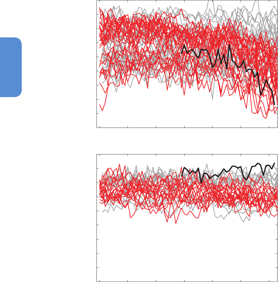
908

Chapter 10 Detection and Attribution of Climate Change: from Global to Regional

Figure 10.16 | September sea ice extent for Arctic (top) and Antarctic (bottom) adaptedfrom (Wang and Overland, 2012). Only CMIP5 models that simulated seasonal mean

and magnitude of seasonal cycle in reasonable agreement with observationsare included in the plot. The grey lines are the runs from the pre-industrial control runs, and the red

lines are from Historical simulations runs patched with RCP8.5 runs for the period of 2005–2012. The black line is based on data from National Snow and Ice Data Center (NSIDC).

There are 24 ensemble members from 11 models for the Arctic and 21 members from 6 models for the Antarctic plot. See Supplementary Material for the precise models used in

the top and bottom panel.

1950 1960 1970 1980 1990 2000 2010

NH40−90N September ice extent

(10

)

Year

(10

)

1950 1960 1970 1980 1990 2000 2010

SH40−90S September ice extent

Several recent studies have investigated the possible causes of Antarctic

sea ice trends. Early studies suggested that stratospheric ozone deple-

tion may have driven increasing trends in Antarctic ice extent (Goosse

et al., 2009; Turner et al., 2009; WMO (World Meteorological Organi-

zation), 2011), but recent studies demonstrate that simulated sea ice

extent decreases in response to prescribed changes in stratospheric

ozone (Sigmond and Fyfe, 2010; Bitz and Polvani, 2012). An alternative

explanation for the lack of melting of Antarctic sea ice is that sub-sur-

face ocean warming, and enhanced freshwater input possibly in part

from ice shelf melting, have made the high-latitude Southern Ocean

fresher (see Section 3.3) and more stratiﬁed, decreasing the upward

heat ﬂux and driving more sea ice formation (Zhang, 2007; Goosse et

al., 2009; Bintanja et al., 2013). An idealized simulation of the response

to freshwater input similar to that estimate due to ice shelf melting

exhibited an increase in sea ice extent (Bintanja et al., 2013), but this

result has yet to be reproduced with other models. Overall we con-

clude that there is low conﬁdence in the scientiﬁc understanding of

the observed increase in Antarctic sea ice extent since 1979, owing to

909

Detection and Attribution of Climate Change: from Global to Regional Chapter 10

the larger differences between sea ice simulations from CMIP5 models

and to the incomplete and competing scientiﬁc explanations for the

causes of change and low conﬁdence in estimates of internal variabil-

ity (Section 9.4.3).

10.5.2 Ice Sheets, Ice Shelves and Glaciers

10.5.2.1 Greenland and Antarctic Ice Sheets

The Greenland and Antarctic ice sheets are important to regional and

global climate because (along with other cryospheric elements) they

cause a polar ampliﬁcation of surface temperatures, a source of fresh

water to the ocean, and represent a source of potentially irrevers-

ible change to the state of the Earth system (Hansen and Lebedeff,

1987). These two ice sheets are important contributors to sea level

rise representing two-thirds of the contributions from all ice covered

regions (Jacob et al., 2012; Pritchard et al., 2012; see Sections 4.4 and

13.3.3). Observations of surface mass balance (increased ablation

versus increased snowfall) are dealt with in Section 4.4.3 and ice sheet

models are discussed in Sections 13.3 and 13.5.

Attribution of change is difﬁcult as ice sheet and glacier changes

are local and ice sheet processes are not generally well represented

in climate models thus precluding formal single-step detection and

attribution studies. However, Greenland observational records show

large recent changes. Section 13.3 concludes that regional models for

Greenland can reproduce trends in the surface mass balance loss quite

well if they are forced with the observed meteorological record, but

not with forcings from a Global Climate Model. Regional model simula-

tions (Fettweis et al., 2013) show that Greenland surface melt increas-

es nonlinearly with rising temperatures due to the positive feedback

between surface albedo and melt.

There have been exceptional changes in Greenland since 2007 marked

by record-setting high air temperatures, ice loss by melting and

marine-terminating glacier area loss (Hanna et al., 2013; Section 4.4.

4). Along Greenland’s west coast temperatures in 2010 and 2011were

the warmest since record keeping began in 1873 resulting in the high-

est observed melt rates in this region since 1958 (Fettweis et al., 2011).

The annual rate of area loss in marine-terminating glaciers was 3.4

times that of the previous 8 years, when regular observations became

available. In 2012, a new record for summertime ice mass loss was two

standard deviations below the 2003–2012 mean, as estimated from

the Gravity Recovery and Climate Experiment (GRACE) satellite (Tedes-

co et al., 2012). The trend of summer mass change during 2003–2012

is rather uniform over this period at –29 ± 11 Gt yr

−1

Record surface melts during 2007–2012 summers are linked to per-

sistent atmospheric circulation that favored warm air advection over

Greenland. These persistent events have changed in frequency since the

beginning of the 2000s (L’Heureux et al., 2010; Fettweis et al., 2011).

Hanna et al. (2013) show a weak relation of Greenland temperatures

and ice sheet runoff with the AMO; they more strongly correlate with

a Greenland atmospheric blocking index. Overland et al. (2012) and

Francis and Vavrus (2012) suggest that the increased frequency of the

Greenland blocking pattern is related to broader scale Arctic changes.

Since 2007, internal variability is likely to have further enhanced the

melt over Greenland. Mass loss and melt is also occurring in Greenland

through the intrusion of warm water into the major glaciers such as

Jacobshaven Glacier (Holland et al., 2008; Walker et al., 2009).

Hanna et al. (2008) attribute increased Greenland runoff and melt since

1990 to global warming; southern Greenland coastal and NH summer

temperatures were uncorrelated between the 1960s and early 1990s

but correlated signiﬁcantly positively thereafter. This relationship was

modulated by the NAO, whose summer index signiﬁcantly negatively

correlated with southern Greenland summer temperatures until the

early 1990s but not thereafter. Regional modelling and observations

tell a consistent story of the response of Greenland temperatures and

ice sheet runoff to shifts in recent regional atmospheric circulation

associated with larger scale ﬂow patterns and global temperature

increases. It is likely that anthropogenic forcing has contributed to sur-

face melting of the Greenland ice sheet since 1993.

There is clear evidence that the West Antarctic ice sheet is contribut-

ing to sea level rise (Bromwich et al., 2013). Estimates of ice mass in

Antarctic since 2000 show that the greatest losses are at the edges

(see Section 4.4). An analysis of observations underneath a ﬂoating ice

shelf off West Antarctica shows that ocean warming and more trans-

port of heat by ocean circulation are largely responsible for increasing

melt rates (Jacobs et al., 2011; Joughin and Alley, 2011; Mankoff et al.,

2012; Pritchard et al., 2012).

Antarctica has regionally dependent decadal variability in surface tem-

perature with variations in these trends depending on the strength of

the SAM climate pattern. Recent warming in continental west Antarc-

tica has been linked to SST changes in the tropical Paciﬁc (Ding et al.,

2011). As with Antarctic sea ice, changes in Antarctic ice sheets have

complex causes (Section 4.4.3). The observational record of Antarctic

mass loss is short and the internal variability of the ice sheet is poorly

understood. Due to a low level of scientiﬁc understanding there is low

conﬁdence in attributing the causes of the observed loss of mass from

the Antarctic ice sheet since 1993. Possible future instabilities in the

west Antarctic ice sheet cannot be ruled out, but projection of future

climate changes over West Antarctica remains subject to considerable

uncertainty (Steig and Orsi, 2013).

10.5.2.2 Glaciers

In the 20th century, there is robust evidence that large-scale internal

climate variability governs interannual to decadal variability in glacier

mass (Hodge et al., 1998; Nesje et al., 2000; Vuille et al., 2008; Huss et

al., 2010; Marzeion and Nesje, 2012) and, along with glacier dynamics,

impacts glacier length as well (Chinn et al., 2005). On time periods

longer than years and decades, there is now evidence of recent ice

loss (see Section 4.3.3) due to increased ambient temperatures and

associated regional moisture changes. However, few studies evaluate

the direct attribution of the current observed mass loss to anthropo-

genic forcing, owing to the difﬁculty associated with contrasting scales

between glaciers and the large-scale atmospheric circulation (Mölg et

al., 2012). Reichert et al. (2002) show for two sample sites at mid and

high latitude that internal climate variability over multiple millennia as

represented in a GCM would not result in such short glacier lengths as

observed in the 20th century. For a sample site at low latitude using

910

Chapter 10 Detection and Attribution of Climate Change: from Global to Regional

multi-step attribution, Mölg et al. (2009) (and references therein) found

a close relation between glacier mass loss and the externally forced

atmosphere–ocean circulation in the Indian Ocean since the late 19th

century. A second, larger group of studies makes use of century-scale

glacier records (mostly glacier length but mass balance as well) to

extract evidence for external drivers. These include local and regional

changes in precipitation and air temperature, and related parameters

(such as melt factors and solid/liquid precipitation ratio) estimated

from the observed change in glaciers. In general these studies show

that the glacier changes reveal unique departures since the 1970s, and

that the inferred climatic drivers in the 20th century and particularly in

most recent decades, exceed the variability of the earlier parts of the

records (Oerlemans, 2005; Yamaguchi et al., 2008; Huss and Bauder,

2009; Huss et al., 2010; Leclercq and Oerlemans, 2011). These results

underline the contrast to former centuries where observed glacier

ﬂuctuations can be explained by internal climate variability (Reichert

et al., 2002; Roe and O’Neal, 2009; Nussbaumer and Zumbühl, 2012).

Anthropogenic land cover change is an unresolved forcing, but a ﬁrst

assessment suggests that it does not confound the impacts of recent

temperature and precipitation changes if the land cover changes are

of local nature (Mölg et al., 2012). The robustness of the estimates

of observed mass loss since the 1960s (Section 4.3, Figure 4.11), the

conﬁdence we have in estimates of natural variations and internal vari-

ability from long-term glacier records, and our understanding of glacier

response to climatic drivers provides robust evidence and, therefore,

high conﬁdence that a substantial part of the mass loss of glaciers is

likely due to human inﬂuence.

10.5.3 Snow Cover

Both satellite and in situ observations show signiﬁcant reductions in

the NH snow cover extent (SCE) over the past 90 years, with most

reduction occurring in the 1980s (see Section 4.5). Formal detection

and attribution studies have indicated anthropogenic inﬂuence on NH

SCE (Rupp et al., 2013) and western USA snow water equivalent (SWE,

Pierce et al., 2008). Pierce et al. (2008) detected anthropogenic inﬂu-

ence in the ratio of 1 April SWE over October to March precipitation

over the period 1950–1999. These reductions could not be explained

by natural internal climate variability alone, nor by changes in solar

and volcanic forcing. In their analysis of NH SCE using 13 CMIP5 sim-

ulations over the 1922–2005 period, Rupp et al. (2013) showed that

some CMIP5 simulations with natural external and anthropogenic

forcings could explain the observed decrease in spring SEC though the

CMIP5 simulations with all forcing as a whole could only explain half

of the magnitude of decrease, and that volcanic and solar variations

(from four CMIP5 simulations) were inconsistent with observations.

We conclude with high conﬁdence in the observational and modelling

evidence that the decrease in NH snow extent since the 1970s is likely

to be caused by all external forcings and has an anthropogenic contri-

bution (see Table 10.1).

10.6 Extremes

Because many of the impacts of climate changes may manifest them-

selves through weather and climate extremes, there is increasing inter-

est in quantifying the role of human and other external inﬂuences on

those extremes. SREX assessed causes of changes in different types

of extremes including temperature and precipitation, phenomena that

inﬂuence the occurrence of extremes (e.g., storms, tropical cyclones),

and impacts on the natural physical environment such as drought (Sen-

eviratne et al., 2012). This section assesses current understanding of

causes of changes in weather and climate extremes, using AR4 as a

starting point. Any changes or modiﬁcations to SREX assessment are

highlighted.

10.6.1 Attribution of Changes in Frequency/

Occurrence and Intensity of Extremes

This sub-section assesses attribution of changes in the characteristics

of extremes including frequency and intensity of extremes. Many of the

extremes discussed in this sub-section are moderate extreme events

that occur more than once in a year (see Box 2.4 for detailed discus-

sion). Attribution of changes in the risk of speciﬁc extreme events,

which are also very rare in general, is assessed in the next sub-section.

10.6.1.1 Temperature Extremes

AR4 concluded that ‘surface temperature extremes have likely been

affected by anthropogenic forcing’. Many indicators of climate

extremes and variability showed changes consistent with warming,

including a widespread reduction in number of frost days in mid-lat-

itude regions and evidence that in many regions warm extremes had

become warmer and cold extremes had become less cold. We next

assess new studies made since AR4.

Relatively warm seasonal mean temperatures (e.g., those that have

a recurrence once in 10 years) have seen a rapid increase in frequen-

cy for many regions worldwide (Jones et al., 2008; Stott et al., 2011;

Hansen et al., 2012) and an increase in the occurrence frequencies of

unusually warm seasonal and annual mean temperatures has been

attributed in part to human inﬂuence (Stott et al., 2011; Christidis et

al., 2012a, 2012b).

A large amount of evidence supports changes in daily data based tem-

perature extreme indices consistent with warming, despite different

data sets or different methods for data processing having been used

(Section 2.6). The effects of human inﬂuence on daily temperature

extremes is suggested by both qualitative and quantitative compar-

isons between observed and CMIP3 based modelled values of warm

days and warm nights (the number of days exceeding the 90th percen-

tile of daily maximum and daily minimum temperatures referred to as

TX90p and TN90p, see also Section 2.7) and cold days and cold nights

(the number of days with daily maximum and daily minimum tem-

peratures below the 10th percentile referred to as TX10p and TN10p;

see also Section 2.7). Trends in temperature extreme indices comput-

ed for Australia (Alexander and Arblaster, 2009) and the USA (Meehl

et al., 2007a) using observations and simulations of the 20th century

with nine GCMs that include both anthropogenic and natural forcings

are found to be consistent. Both observations and model simulations

show a decrease in the number of frost days, and an increase in the

growing season length, heatwave duration and TN90p in the second

half of the 20th century. Two of the models (PCM and CCSM3) with

simulations that include only anthropogenic or only natural forcings

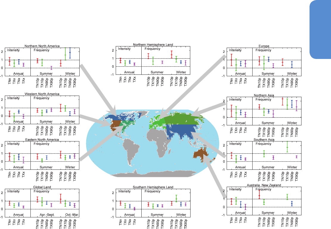
911

Detection and Attribution of Climate Change: from Global to Regional Chapter 10

indicate that the observed changes are simulated with anthropogenic

forcings, but not with natural forcings (even though there are some

differences in the details of the forcings). Morak et al. (2011) found

that over many sub-continental regions, the number of warm nights

(TN90p) shows detectable changes over the second half of the 20th

century that are consistent with model simulated changes in response

to historical external forcings. They also found detectable changes in

indices of temperature extremes when the data were analysed over

the globe as a whole. As much of the long-term change in TN90p

can be predicted based on the interannual correlation of TN90p with

mean temperature, Morak et al. (2013) conclude that the detectable

changes are attributed in a multi-step approach (see Section 10.2.4)

in part to GHG increases. Morak et al. (2013) have extended this anal-

ysis to TX10p, TN10p, TX90p as well as TN90p, using ﬁngerprints from

HadGEM1 and ﬁnd detectable changes on global scales and in many

regions (Figure 10.17).

Human inﬂuence has also been detected in two different measures

of the intensity of extreme daily temperatures in a year. Zwiers et al.

(2011) compared four extreme temperature variables including warm-

est daily maximum and minimum temperatures (annual maximum

Figure 10.17 | Detection results for changes in intensity and frequency of extreme events. The left side of each panel shows scaling factors and their 90% conﬁdence intervals for

intensity of annual extreme temperatures in response to external forcings for the period 1951–2000. TNn and TXn represent coldest daily minimum and maximum temperatures,

respectively, while TNx and TXx represent warmest daily minimum and maximum temperatures (updated from Zwiers et al., 2011). Fingerprints are based on simulations of climate

models with both anthropogenic and natural forcings. Right-hand sides of each panel show scaling factors and their 90% conﬁdence intervals for changes in the frequency of

temperature extremes for winter (October to March for the Northern Hemisphere and April to September for the Southern Hemisphere), and summer half years. TN10p, TX10p are

respectively the frequency of cold nights and days (daily minimum and daily maximum temperatures falling below their 10th percentiles for the base period 1961–1990). TN90p

and TX90p are the frequency of warm nights and days (daily minimum and daily maximum temperatures above their respective 90th percentiles calculated for the 1961–1990

base period (Morak et al., 2013) with ﬁngerprints based on simulations of Hadley Centre Global Environmental Model 1 (HadGEM1) with both anthropogenic and natural forcings.

Detection is claimed at the 5% signiﬁcance level if the 90% conﬁdence interval of a scaling factor is entirely above the zero line. Grey represents regions with insufﬁcient data.

daily maximum and minimum temperatures, referred to as TXx, TNx)

and coldest daily maximum and minimum temperatures (annual

minimum daily maximum and minimum temperatures, referred to as

TXn, TNn) from observations and from simulations with anthropogen-

ic forcing or anthropogenic and natural external forcings from seven

GCMs. They consider these extreme daily temperatures to follow gen-

eralized extreme value (GEV) distributions with location, shape and

scale parameters. They ﬁt GEV distributions to the observed extreme

temperatures with location parameters as linear functions of signals

obtained from the model simulation. They found that both anthropo-

genic inﬂuence and combined inﬂuence of anthropogenic and natural

forcing can be detected in all four extreme temperature variables at

the global scale over the land, and also regionally over many large

land areas (Figure 10.17). In a complementary study, Christidis et al.

(2011) used an optimal ﬁngerprint method to compare observed and

modelled time-varying location parameters of extreme temperature

distributions. They detected the effects of anthropogenic forcing on

warmest daily temperatures in a single ﬁngerprint analysis, and were

able to separate the effects of natural from anthropogenic forcings in

a two ﬁngerprint analysis.

912

Chapter 10 Detection and Attribution of Climate Change: from Global to Regional

Human inﬂuence on annual extremes of daily temperatures may be

detected separately from natural forcing at the global scale (Christidis

et al., 2011) and also at continental and sub-continental scales (Min

et al., 2013). Over China, Wen et al. (2013) showed that anthropo-

genic inﬂuence may be separately detected from that of natural forc-

ing in daily extreme temperatures (TNn, TNx, TXn and TXx), although

the inﬂuence of natural forcing is not detected, and they also showed

that the inﬂuence of GHGs in these indices may be separately detect-

ed from other anthropogenic forcings. Christidis et al. (2013) found

that on a quasi-global scale, the cooling effect due to the decrease

in tree cover and increase in grass cover since pre-industrial times as

simulated by one ESM is detectable in the observed change of warm

extremes. Urbanization may have also affected extreme temperatures

in some regions; for example Zhou and Ren (2011) found that extreme

temperature warms more in rural stations than in urban sites in China.

The effect of land use change and urban heat Island is found to be

small in GMST (Section 2.4.1.3). Consequently, this effect on extreme

temperature is also expected to be small in the global average.

These new studies show that there is stronger evidence for anthropo-

genic forcing on changes in extreme temperatures than at the time of

the SREX assessment. New evidence since SREX includes the separation

of the inﬂuence of anthropogenic forcings from that of natural forcings

on extreme daily temperatures at the global scale and to some extent

at continental and sub-continental scales in some regions. These new

results suggest more clearly the role of anthropogenic forcing on tem-

perature extremes compared to results at the time of the SREX assess-

ment. We assess that it is very likely that human inﬂuence has contrib-

uted to the observed changes in the frequency and intensity of daily

temperature extremes on the global scale since the mid-20th century.

10.6.1.2 Precipitation Extremes

Observations have showed a general increase in heavy precipitation

at the global scale. This appears to be consistent with the expected

response to anthropogenic forcing as a result of an enhanced moisture

content in the atmosphere but a direct cause-and-effect relationship

between changes in external forcing and extreme precipitation had

not been established at the time of the AR4. As a result, the AR4 con-

cluded that increases in heavy precipitation were more likely than not

consistent with anthropogenic inﬂuence during the latter half of the

20th century (Hegerl et al., 2007b).

Extreme precipitation is expected to increase with warming. A com-

bination of evidence leads to this conclusion though by how much

remains uncertain and may vary with time scale (Section 7.6.5). Obser-

vations and model projected future changes both indicate increase in

extreme precipitation associated with warming. Analysis of observed

annual maximum 1-day precipitation (RX1day) over global land areas

with sufﬁcient data smaples indicates a signiﬁcant increase in extreme

percipitation globally, with a median increase about 7% °C

–1

GMST

increase (Westra et al., 2013). CMIP3 and CMIP5 simulations project

an increase in the globally averaged 20-year return values of annual

maximum 24-hour precipitation amounts of about 6 to 7% with each

degree Celsius of global mean warming, with the bulk of models sim-

ulating values in the range of 4 to 10% °C

–1

(Kharin et al., 2007; Kharin

et al., 2013). Anthropogenic inﬂuence has been detected on various

aspects of the global hydrological cycle (Stott et al., 2010), which is

directly relevant to extreme precipitation changes. An anthropogen-

ic inﬂuence on increasing atmospheric moisture content has been

detected (see Section 10.3.2). A higher moisture content in the atmos-

phere would be expected to lead to stronger extreme precipitation as

extreme precipitation typically scales with total column moisture if cir-

culation does not change. An observational analysis shows that winter

maximum daily precipitation in North America has statistically signiﬁ-

cant positive correlations with local atmospheric moisture (Wang and

Zhang, 2008).

There is only a modest body of direct evidence that natural or anthro-

pogenic forcing has affected global mean precipitation (see Section

10.3.2 and Figure 10.10), despite a robust expectation of increased

precipitation (Balan Sarojini et al., 2012 ) and precipitation extremes

(see Section 7.6.5). However, mean precipitation is expected to

increase less than extreme precipitation because of energy constraints

(e.g., Allen and Ingram, 2002). A perfect model analysis with an ensem-

ble of GCM simulations shows that anthropogenic inﬂuence should

be detectable in precipitation extremes in the second half of the 20th

century at global and hemispheric scales, and at continental scale as

well but less robustly (Min et al., 2008c), see also Hegerl et al. (2004).

One study has also linked the observed intensiﬁcation of precipitation

extremes (including RX1day and annual maximum 5-day precipitation

(RX5day)) over NH land areas to human inﬂuence using a limited set

of climate models and observations (Min et al., 2011). However, the

detection was less robust if using the ﬁngerprint for combined anthro-

pogenic and natural inﬂuences compared to that for anthropogenic

inﬂuences only, possibly due to a number of factors including weak

S/N ratio and uncertainties in observation and model simulations. Also,

models still have difﬁculties in simulating extreme daily precipitation

directly comparable with those observed at the station level, which has

been addressed to some extent by Min et al. (2011) by independently

transforming annual precipitation extremes in models and observations

onto a dimensionless scale that may be more comparable between the

two. Detection of anthropogenic inﬂuence on smaller spatial scales

is more difﬁcult due to the increased level of noise and uncertainties

and confounding factors on local scales. Fowler and Wilby (2010) sug-

gested that there may have only been a 50% likelihood of detecting

anthropogenic inﬂuence on UK extreme precipitation in winter at that

time, and a very small likelihood of detecting it in other seasons.

Given the evidence of anthropogenic inﬂuence on various aspects of

the global hydrological cycle that implies that extreme precipitation

would be expected to have increased and some limited direct evidence

of anthropogenic inﬂuence on extreme precipitation, but given also the

difﬁculties in simulating extreme precipitation by climate models and

limited observational coverage, we assess, consistent with SREX (Sen-

eviratne et al., 2012) that there is medium conﬁdence that anthropo-

genic forcing has contributed to a global scale intensiﬁcation of heavy

precipitation over the second half of the 20th century in land regions

where observational coverage is sufﬁcient for assessment.

10.6.1.3 Drought

AR4 concluded that that an increased risk of drought was more likely

than not due to anthropogenic forcing during the second half of the

913

Detection and Attribution of Climate Change: from Global to Regional Chapter 10

20th century. This assessment was based on one detection study that

identiﬁed an anthropogenic ﬁngerprint in a global Palmer Drought

Severity Index (PDSI) data set (Burke et al., 2006) and studies of some

regions which indicated that droughts in those regions were linked

to SST changes or to a circulation response to anthropogenic forcing.

SREX (Seneviratne et al., 2012) assessed that there was medium conﬁ-

dence that anthropogenic inﬂuence has contributed to some changes

in the drought patterns observed in the second half of the 20th century

based on attributed impact of anthropogenic forcing on precipitation

and temperature changes, and that there was low conﬁdence in the

assessment of changes in drought at the level of single regions.

Drought is a complex phenomenon that is affected by precipitation

predominantly, as well as by other climate variables including temper-

ature, wind speed and solar radiation (e.g., Seneviratne, 2012; Shef-

ﬁeld et al., 2012). It is also affected by non-atmospheric conditions

such as antecedent soil moisture and land surface conditions. Trends

in two important drought-related climate variables (precipitation and

temperature) are consistent with the expected responses to anthro-

pogenic forcing over the globe. However, there is large uncertainty

in observed changes in drought (Section 2.6.2.3) and its attribution

to causes globally. The evidence for changes in soil moisture indices

and drought indices over the period since 1950 globally is conﬂicting

(Hoerling et al., 2012; Shefﬁeld et al., 2012; Dai, 2013), possibly due to

the examination of different time periods, different forcing ﬁelds used

to drive land surface models and uncertainties in land surface models

(Pitman et al., 2009; Seneviratne et al., 2010; Shefﬁeld et al., 2012).

In a recent study, Shefﬁeld et al. (2012) identify the representation

of potential evaporation as solely dependent on temperature (using

the Thornthwaite-based formulation) as a possible explanation for

their ﬁnding that PDSI-based estimates might overestimate historical

drought trends. This stands in partial contradiction to previous assess-

ments suggesting that using a more sophisticated formulation (Pen-

man-Monteith) for potential evaporation did not affect the results of

respective PDSI trends (Dai, 2011; van der Schrier et al., 2011). Shefﬁeld

et al. (2012) argue that issues with the treatment of spurious trends in

atmospheric forcing data sets and/or the choice of calibration periods

explain these conﬂicting results. These conﬂicting results point out the

challenges in quantitatively deﬁning and detecting long-term changes

in a multivariable phenomenon such as drought.

Recent long-term droughts in western North America cannot deﬁni-

tively be shown to lie outside the very large envelope of natural precip-

itation variability in this region (Cayan et al., 2010; Seager et al., 2010),

particularly given new evidence of the history of high-magnitude nat-

ural drought and pluvial episodes suggested by palaeoclimatic recon-

structions (see Chapter 5). Low-frequency tropical ocean temperature

anomalies in all ocean basins appear to force circulation changes that

promote regional drought (Hoerling and Kumar, 2003; Seager et al.,

2005; Dai, 2011). Uniform increases in SST are not particularly effective

in this regard (Schubert et al., 2009; Hoerling et al., 2012). Therefore,

the reliable separation of natural variability and forced climate change

will require simulations that accurately reproduce changes in large-

scale SST gradients at all time scales.

In summary, assessment of new observational evidence, in conjunc-

tion with updated simulations of natural and forced climate varia-

bility, indicates that the AR4 conclusions regarding global increasing

trends in droughts since the 1970s should be tempered. There is not

enough evidence to support medium or high conﬁdence of attribution

of increasing trends to anthropogenic forcings as a result of observa-

tional uncertainties and variable results from region to region (Section

2.6.2.3). Combined with difﬁculties described above in distinguishing

decadal scale variability in drought from long-term climate change we

conclude consistent with SREX that there is low conﬁdence in detec-

tion and attribution of changes in drought over global land areas since

the mid-20th century.

10.6.1.4 Extratropical Cyclones

AR4 concluded that an anthropogenic inﬂuence on extratropical

cyclones was not formally detected, owing to large internal variability

and problems due to changes in observing systems. Although there

is evidence that there has been a poleward shift in the storm tracks

(see Section 2.6.4), various causal factors have been cited including

oceanic heating (Butler et al., 2010) and changes in large-scale cir-

culation due to effects of external forcings (Section 10.3.3). Increases

in mid-latitude SST gradients generally lead to stronger storm tracks

that are shifted poleward and increases in subtropical SST gradients

may lead to storm tracks shifting towards the equator (Brayshaw et

al., 2008; Semmler et al., 2008; Kodama and Iwasaki, 2009; Graff and

LaCasce, 2012). However, changes in storm-track intensity are much

more complicated, as they are sensitive to the competing effects of

changes in temperature gradients and static stability at different levels

and are thus not linked to GMST in a simple way (Ulbrich et al., 2009;

O’Gorman, 2010). Overall global average cyclone activity is expected

to change little under moderate GHG forcing (O’Gorman and Schnei-

der, 2008; Ulbrich et al., 2009; Bengtsson and Hodges, 2011), although

in one study, human inﬂuence has been detected in geostrophic wind

energy and ocean wave heights derived from sea level pressure data

(Wang et al., 2009b).

10.6.1.5 Tropical Cyclones

AR4 concluded that ‘anthropogenic factors more likely than not have

contributed to an increase in tropical cyclone intensity’ (Hegerl et al.,

2007b). Evidence that supports this assessment was the strong correla-

tion between the Power Dissipation Index (PDI, an index of the destruc-

tiveness of tropical cyclones) and tropical Atlantic SSTs (Emanuel,

2005; Elsner, 2006) and the association between Atlantic warming and

the increase in GMST (Mann and Emanuel, 2006; Trenberth and Shea,

2006). Observations suggest an increase globally in the intensities of

the strongest tropical cyclones (Elsner et al., 2008) but it is difﬁcult

to attribute such changes to particular causes (Knutson et al., 2010).

The US Climate Change Science Program (CCSP; Kunkel et al., 2008)

discussed human contributions to recent hurricane activity based on

a two-step attribution approach. They concluded merely that it is very

likely (Knutson et al., 2010) that human-induced increase in GHGs has

contributed to the increase in SSTs in the hurricane formation regions

and that over the past 50 years there has been a strong statistical

connection between tropical Atlantic SSTs and Atlantic hurricane activ-

ity as measured by the PDI. Knutson et al. (2010), assessed that ‘…it

remains uncertain whether past changes in tropical cyclone activity

have exceeded the variability expected from natural causes.’ Senevi-

914

Chapter 10 Detection and Attribution of Climate Change: from Global to Regional

ratne et al. (2012) concurred with this ﬁnding. Section 14.6.1 gives a

detailed account of past and future changes in tropical cyclones. This

section assesses causes of observed changes.

Studies that directly attribute tropical cyclone activity changes to

anthropogenic GHG emission are lacking. Among many factors that

may affect tropical cyclone activity, tropical SSTs have increased and

this increase has been attributed at least in part to anthropogen-

ic forcing (Gillett et al., 2008a). However, there are diverse views on

the connection between tropical cyclone activity and SST (see Section

14.6.1 for details). Strong correlation between the PDI and tropical

Atlantic SSTs (Emanuel, 2005; Elsner, 2006) would suggest an anthro-

pogenic inﬂuence on tropical cyclone activity. However, recent stud-

ies also suggest that regional potential intensity correlates with the

difference between regional SSTs and spatially averaged SSTs in the

tropics (Vecchi and Soden, 2007; Xie et al., 2010; Ramsay and Sobel,

2011) and projections are uncertain on whether the relative SST will

increase over the 21st century under GHG forcing (Vecchi et al., 2008;

Xie et al., 2010; Villarini and Vecchi, 2012, 2013) . Analyses of CMIP5

simulations suggest that while PDI over the North Atlantic is project-

ed to increase towards late 21st century no detectable change in PDI

should be present in the 20th century (Villarini and Vecchi, 2013) . On

the other hand, Emanuel et al. (2013) point out that while GCM hind-

casts indeed predict little change over the 20th century, downscaling

driving by reanalysis data that incorporate historical observations are

in much better accord with observations and do indicate a late 20th

century increase.

Some recent studies suggest that the reduction in the aerosol forcing

(both anthropogenic and natural) over the Atlantic since the 1970s

may have contributed to the increase in tropical cyclone activity in the

region (see Section 14.6.1 for details), and similarly that aerosols may

have acted to reduce tropical cyclone activity in the Atlantic in ear-

lier years when aerosol forcing was increasing (Villarini and Vecchi,

2013). However, there are different views on the relative contribution

of aerosols and decadal natural variability of the climate system to

the observed changes in Atlantic tropical cyclone activity among these

studies. Some studies indicate that aerosol changes have been the

main driver (Mann and Emanuel, 2006; Evan et al., 2009; Booth et al.,

2012; Villarini and Vecchi, 2012, 2013). Other studies infer the inﬂu-

ence of natural variability to be as large as or larger than that from

aerosols (Zhang and Delworth, 2009; Villarini and Vecchi, 2012, 2013).

Globally, there is low conﬁdence in any long-term increases in tropical

cyclone activity (Section 2.6.3) and we assess that there is low con-

ﬁdence in attributing global changes to any particular cause. In the

North Atlantic region there is medium conﬁdence that a reduction in

aerosol forcing over the North Atlantic has contributed at least in part

to the observed increase in tropical cyclone activity since the 1970s.

There remains substantial disagreement on the relative importance of

internal variability, GHG forcing and aerosols for this observed trend.

It remains uncertain whether past changes in tropical cyclone activity

are outside the range of natural internal variability.

10.6.2 Attribution of Weather and Climate Events

Since many of the impacts of climate change are likely to manifest

themselves through extreme weather, there is increasing interest in

quantifying the role of human and other external inﬂuences on climate

in speciﬁc weather events. This presents particular challenges for both

science and the communication of results. It has so far been attempted

for a relatively small number of speciﬁc events (e.g., Stott et al., 2004;

Pall et al., 2011) although Peterson et al. (2012) attempt, for the ﬁrst

time, a coordinated assessment to place different high-impact weather

events of the previous year in a climate perspective. In this assessment,

selected studies are used to illustrate the essential principles of event

attribution: see Stott et al. (2013) for a more exhaustive review.

Two distinct ways have emerged of framing the question of how an

external climate driver like increased GHG levels may have contributed

to an observed weather event. First, the ‘attributable risk’ approach

considers the event as a whole, and asks how the external driver

may have increased or decreased the probability of occurrence of an

event of comparable magnitude. Second, the ‘attributable magnitude’

approach considers how different external factors contributed to the

event or, more speciﬁcally, how the external driver may have increased

the magnitude of an event of comparable occurrence probability. Hoer-

ling et al. (2013) uses both methods to infer changes in magnitude and

likelihood of the 2011 Texas heat wave.

Quantifying the absolute risk or probability of an extreme weather

event in the absence of human inﬂuence on climate is particularly

challenging. Many of the most extreme events occur because a self-re-

inforcing process that occurs only under extreme conditions ampliﬁes

an initial anomaly (e.g., Fischer et al., 2007). Hence the probability of

occurrence of such events cannot, in general, be estimated simply by

extrapolating from the distribution of less extreme events that are

sampled in the historical record. Proxy records of pre-industrial climate

generally do not resolve high-frequency weather, so inferring changes

in probabilities requires a combination of hard-to-test distributional

assumptions and extreme value theory. Quantifying absolute probabil-

ities with climate models is also difﬁcult because of known biases in

their simulation of extreme events. Hence, with only a couple of excep-

tions (e.g., Hansen et al., 2012), studies have focussed on how risks

have changed or how different factors have contributed to an observed

event, rather than claiming that the absolute probability of occurrence

of that event would have been extremely low in the absence of human

inﬂuence on climate.

Even without considering absolute probabilities, there remain con-

siderable uncertainties in quantifying changes in probabilities. The

assessment of such changes will depend on the selected indicator, time

period and spatial scale on which the event is analysed, and the way in

which the event-attribution question is framed can substantially affect

apparent conclusions . If an event occurs in the tail of the distribution,

then a small shift in the distribution as a whole can result in a large

increase in the probability of an event of a given magnitude: hence it

is possible for the same event to be both ‘mostly natural’ in terms of

attributable magnitude (if the shift in the distribution due to human

inﬂuence is small compared to the anomaly in the natural variability

that was the primary cause) and ‘mostly anthropogenic’ in terms of

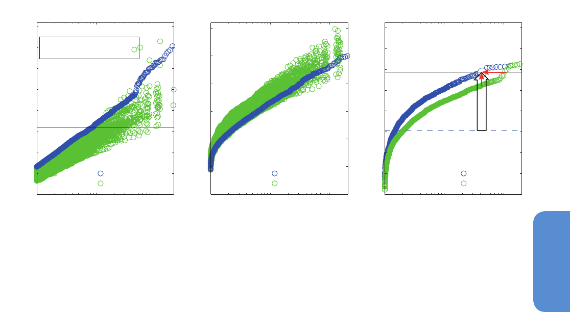
915

Detection and Attribution of Climate Change: from Global to Regional Chapter 10

attributable risk (if human inﬂuence has increased its probability of

occurrence by more than a factor of 2). These issues are discussed fur-

ther using the example of the 2010 Russian heat wave below.

The majority of studies have focussed on quantifying attributable risk.

Formally, risk is a function of both hazard and vulnerability (IPCC,

2012), although most studies attempting to quantify risk in the con-

text of extreme weather do not explicitly use this deﬁnition, which is

discussed further in Chapter 19 of WGII, but use the term as a short-

hand for the probability of the occurrence of an event of a given mag-

nitude. Any assessment of change in risk depends on an assumption

of ‘all other things being equal’, including natural drivers of climate

change and vulnerability. Given this assumption, the change in hazard

is proportional to the change in risk, so we will follow the published

literature and continue to refer to Fraction Attributable Risk, deﬁned

as FAR = 1 – P0/P1, P0 being the probability of an event occurring in

the absence of human inﬂuence on climate, and P1 the corresponding

probability in a world in which human inﬂuence is included. FAR is

thus the fraction of the risk that is attributable to human inﬂuence (or,

potentially, any other external driver of climate change) and does not

require knowledge of absolute values of P0 and P1, only their ratio.

For individual events with return times greater than the time scale

over which the signal of human inﬂuence is emerging (30 to 50 years,

meaning P0 and P1 less than 2 to 3% in any given year), it is impossi-

ble to observe a change in occurrence frequency directly because of the

shortness of the observed record, so attribution is necessarily a mul-

ti-step procedure. Either a trend in occurrence frequency of more fre-

quent events is attributed to human inﬂuence and a statistical model

is then used to extrapolate to the implications for P0 and P1; or an

attributable trend is identiﬁed in some other variable, such as surface

temperature, and a physically based weather model is used to assess

the implications for extreme weather risk. Neither approach is free of

assumptions: no atmospheric model is perfect, but statistical extrapo-

lation may also be misleading for reasons given above.

Pall et al. (2011) provide an example of multi-step assessment of

attributable risk using a physically based model, applied to the ﬂoods

that occurred in the UK in the autumn of 2000, the wettest autumn

to have occurred in England and Wales since records began. To assess

the contribution of the anthropogenic increase in GHGs to the risk of

these ﬂoods, a several thousand member ensemble of atmospheric

models with realistic atmospheric composition, SST and sea ice bound-

ary conditions imposed was compared with a second ensemble with

composition and surface temperatures and sea ice boundary condi-

tions modiﬁed to simulate conditions that would have occurred had

there been no anthropogenic increase in GHGs since 1900. Simulated

daily precipitation from these two ensembles was fed into an empirical

rainfall-runoff model and daily England and Wales runoff used as a

proxy for ﬂood risk. Results (Figure 10.18a) show that including the

inﬂuence of anthropogenic greenhouse warming increases ﬂood risk

at the threshold relevant to autumn 2000 by around a factor of two in

the majority of cases, but with a broad range of uncertainty: in 10% of

cases the increase in risk is less than 20%.

Kay et al. (2011a), analysing the same ensembles but using a more

sophisticated hydrological model found a reduction in the risk of snow

melt–induced ﬂooding in the spring season (Figure 10.18b) which,

aggregated over the entire year, largely compensated for the increased

risk of precipitation-induced ﬂooding in autumn. This illustrates an

Return time (yr)

Daily runoff in (mm day

-1

)

a) Autumn runoff, England and Wales

10% 1%

Chance of exceeding

threshold in a given year

1 10 100

0.25

0.3

0.35

0.4

0.45

0.5

0.55

0.6

0.65

Autumn 2000

Non−industrial

10%1%

Return time (yr)

Daily peak flow in (m

-1

)

b) Spring flow, River Don, UK

1 10 100

100

150

200

250

300

Spring 2001

Non−industrial

Return time (yr)

Monthly temperature equivalent in (°C)

c) July temperatures, Western Russia

1 10 100

2000−2009

1960−1969

Figure 10.18 | Return times for precipitation-induced ﬂoods aggregated over England and Wales for (a) conditions corresponding to September to November 2000 with bound-

ary conditions as observed (blue) and under a range of simulations of the conditions that would have obtained in the absence of anthropogenic greenhouse warming over the

20th century (green) with different AOGCMs used to deﬁne the greenhouse signal, black horizontal line corresponds to the threshold exceeded in autumn 2000 (from Pall et al.,

2011); (b) corresponding to January to March 2001 with boundary conditions as observed (blue) and under a range of simulations of the condition that would have obtained in the

absence of anthropogenic greenhouse warming over the 20th century (green) adapted from Kay et al. (2011a); (c) return periods of temperature-geopotential height conditions in

the model simulations for the 1960s (green) and the 2000s (blue). The vertical black arrow shows the anomaly of the 2010 Russian heat wave (black horizontal line) compared to

the July mean temperatures of the 1960s (dashed line). The vertical red arrow gives the increase in temperature for the event whereas the horizontal red arrow shows the change

in the return period (from Otto et al., 2012).

916

Chapter 10 Detection and Attribution of Climate Change: from Global to Regional

important general point: even if a particular ﬂood event may have

been made more likely by human inﬂuence on climate, there is no cer-

tainty that all kinds of ﬂood events in that location, country or region

have been made more likely.

Rahmstorf and Coumou (2011) provide an example of an empirical

approach to the estimation of attributable risk applied to the 2010

Russian heat wave. They ﬁt a nonlinear trend to central Russian tem-

peratures and show that the warming that has occurred in this region

since the 1960s has increased the risk of a heat wave of the mag-

nitude observed in 2010 by around a factor of 5, corresponding to

an FAR of 0.8. They do not address what has caused the trend since

1960, although they note that other studies have attributed most of

the large-scale warming over this period to the anthropogenic increase

in GHG concentrations.

Dole et al. (2011) take a different approach to the 2010 Russian heat

wave, focussing on attributable magnitude, analysing contributions

from various external factors, and conclude that this event was ‘mainly

natural in origin’. First, observations show no evidence of a trend in

occurrence frequency of hot Julys in western Russia, and despite the

warming that has occurred since the 1960s, mean July temperatures in

that region actually display a (statistically insigniﬁcant) cooling trend

over the century as a whole, in contrast to the case for central and

southern European summer temperatures (Stott et al., 2004). Mem-

bers of the CMIP3 multi-model ensemble likewise show no evidence

of a trend towards warming summers in central Russia. Second, Dole

et al. (2011) note that the 2010 Russian event was associated with

a strong blocking atmospheric ﬂow anomaly, and even the complete

2010 boundary conditions are insufﬁcient to increase the probability

of a prolonged blocking event in this region, in contrast again to the

situation in Europe in 2003. This anomaly in the large-scale atmos-

pheric ﬂow led to low-pressure systems being redirected around the

blocking over Russia causing severe ﬂooding in Pakistan which could

so far not be attributed to anthropogenic causes (van Oldenborgh et

al., 2012), highlighting that a global perspective is necessary to unravel

the different factors inﬂuencing individual extreme events (Trenberth

and Fasullo, 2012).

Otto et al. (2012) argue that it is possible to reconcile the results of

Rahmstorf and Coumou (2011) with those of Dole et al. (2011) by

relating the attributable risk and attributable magnitude approaches

to framing the event attribution question. This is illustrated in Figure

10.18c, which shows return times of July temperatures in western

Russia in a large ensemble of atmospheric model simulations for the

1960s (in green) and 2000s (in blue). The threshold exceeded in 2010

is shown by the solid horizontal line which is almost 6°C above 1960s

mean July temperatures, shown by the dashed line. The difference

between the green and blue lines could be characterized as a 1.5°C

increase in the magnitude of a 30-year event (the vertical red arrow,

which is substantially smaller than the size of the anomaly itself, sup-

porting the assertion that the event was ‘mainly natural’ in terms of

attributable magnitude. Alternatively, it could be characterized as a

threefold increase in the risk of the 2010 threshold being exceeded,

supporting the assertion that risk of the event occurring was mainly

attributable to the external trend, consistent with Rahmstorf and

Coumou (2011). Rupp et al. (2012) and Hoerling et al. (2013) reach

similar conclusions about the 2011 Texas heat wave, both noting the

importance of La Niña conditions in the Paciﬁc, with anthropogenic

warming making a relatively small contribution to the magnitude of

the event, but a more substantial contribution to the risk of temper-

atures exceeding a high threshold. This shows that the quantiﬁcation

of attributable risks and and changes in magnitude are affected by

modelling error (e.g., Visser and Petersen, 2012) as they depend on the

atmospheric model’s ability to simulate the observed anomalies in the

general circulation (Chapter 9).

Because much of the magnitude of these two heat waves is attrib-

utable to atmospheric ﬂow anomalies, any evidence of a causal link

between rising GHGs and the occurrence or persistence of ﬂow anom-

alies such as blocking would have a very substantial impact on attri-

bution claims. Pall et al. (2011) argue that, although ﬂow anomalies

played a substantial role in the autumn 2000 ﬂoods in the UK, thermo-

dynamic mechanisms were primarily responsible for the change in risk

between their ensembles. Regardless of whether the statistics of ﬂow

regimes themselves have changed, observed temperatures in recent

years in Europe are distinctly warmer than would be expected for anal-

ogous atmospheric ﬂow regimes in the past, affecting both warm and

cold extremes (Yiou et al., 2007; Cattiaux et al., 2010).

In summary, increasing numbers of studies are ﬁnding that the prob-

ability of occurrence of events associated with extremely high tem-

peratures has increased substantially due to the large-scale warming

since the mid-20th century. Because most of this large-scale warming

is very likely due to the increase in atmospheric GHG concentrations, it

is possible to attribute, via a multi-step procedure, some of the increase

in probability of these regional events to human inﬂuence on climate.

Such an increase in probability is consistent with the implications of

single-step attribution studies looking at the overall implications of

increasing mean temperatures for the probabilities of exceeding tem-

perature thresholds in some regions. We conclude that it is likely that

human inﬂuence has substantially increased the probability of occur-

rence of heat waves in some locations. It is expected that attributable

risks for extreme precipitation events are generally smaller and more

uncertain, consistent with the ﬁndings in Kay et al. (2011a) and Pall

et al. (2011). The science of event attribution is still conﬁned to case

studies, often using a single model, and typically focussing on high-im-

pact events for which the issue of human inﬂuence has already arisen.

While the increasing risk of heat waves measured as the occurrence of

a previous temperature record being exceeded can simply be explained

by natural variability superimposed by globally increasing temperature,

conclusions for holistic events including general circulation patterns

are speciﬁc to the events that have been considered so far and rely on

the representation of relevant processes in the model.

Anthropogenic warming remains a relatively small contributor to the

overall magnitude of any individual short-term event because its mag-

nitude is small relative to natural random weather variability on short

time scales (Dole et al., 2011; Hoerling et al., 2013). Because of this

random variability, weather events continue to occur that have been

made less likely by human inﬂuence on climate, such as extreme winter

cold events (Massey et al., 2012), or whose probability of occurrence

has not been signiﬁcantly affected either way. Quantifying how dif-

ferent external factors contribute to current risks, and how risks are

917

Detection and Attribution of Climate Change: from Global to Regional Chapter 10

changing, is possible with much higher conﬁdence than quantifying

absolute risk. Biases in climate models, uncertainty in the probability

distribution of the most extreme events and the ambiguity of paleocli-

matic records for short-term events mean that it is not yet possible to

quantify the absolute probability of occurrence of any observed weath-

er event in a hypothetical pristine climate. At present, therefore, the

evidence does not support the claim that we are observing weather

events that would, individually, have been extremely unlikely in the

absence of human-induced climate change, although observed trends

in the concurrence of large numbers of events (see Section 10.6.1)

may be more easily attributable to external factors. The most impor-

tant development since AR4 is an emerging consensus that the role of

external drivers of climate change in speciﬁc extreme weather events,

including events that might have occurred in a pre-industrial climate,

can be quantiﬁed using a probabilistic approach.

10.7 Multi-century to Millennia Perspective

Evaluating the causes of climate change before the 20th century is

important to test and improve our understanding of the role of inter-

nal and forced natural climate variability for the recent past. This sec-

tion draws on assessment of temperature reconstructions of climate

change over the past millennium and their uncertainty in Chapter 5

(Table 5.A.1; Sections 5.3.5 and 5.5.1 for regional records), and on

comparisons of models and data over the pre-instrumental period in

Chapters 5 and 9 (Sections 5.3.5, 5.5.1 and 9.5.3), and focuses on the

evidence for the contribution by radiatively forced climate change to

reconstructions and early instrumental records. In addition, the residual

variability that is not explained by forcing from palaeoclimatic records

provides a useful comparison to estimates of climate model internal

variability. The model dependence of estimates of internal variability is

an important uncertainty in detection and attribution results.

The inputs for detection and attribution studies for periods covered by

indirect, or proxy, data are affected by more uncertainty than those

from the instrumental period (see Chapter 5), owing to the sparse data

coverage, particularly further back in time, and uncertainty in the link

between proxy data and, for example, temperature. Records of past

radiative inﬂuences on climate are also uncertain (Section 5.2; see

Schmidt et al., 2011; Schmidt et al., 2012). For the preindustrial part of

the last millennium changes in solar, volcanic, GHG forcing, and land

use change, along with a small orbital forcing are potentially important

external drivers of climate change. Estimates of solar forcing (Figure

5.1a; Box 10.2) are uncertain, particularly in their amplitude, as well as

in modelling, for example, of the inﬂuence of solar forcing on atmos-

pheric circulation involving stratospheric dynamics (see Box 10.2; Gray

et al., 2010). Estimates of past volcanism are reasonably well estab-

lished in their timing, but the magnitude of the RF of individual erup-

tions is uncertain (Figure 5.1a). It is possible that large eruptions had a

more moderated climate effect than simulated by many climate models

due to faster fallout associated with larger particle size (Timmreck et

al., 2009), or increased amounts of injected water vapour (Joshi and

Jones, 2009). Reconstructed changes in land cover and its effect on

climate are also uncertain (Kaplan et al., 2009; Pongratz et al., 2009).

Forcing of WMGHGs shows only very subtle variations over the last

millennium up to 1750. This includes a small drop and partial recovery

in the 17th century (Section 6.2.3, Figure 6.7), followed by increases in

GHG concentrations with industrialization since the middle of the 18th

century (middle of the 19th century for N

O, Figure 6.11).

When interpreting reconstructions of past climate change with the help

of climate models driven with estimates of past forcing, it helps that

the uncertainties in reconstructions and forcing are independent from

each other. Thus, uncertainties in forcing and reconstructions combined

should lead to less, rather than more similarity between ﬁngerprints

of forced climate change and reconstructions, making it improbable

that the response to external drivers is spuriously detected. Howev-

er, this is the case only if all relevant forcings and their uncertainties

are considered, reducing the risk of misattribution due to spurious

correlations between external forcings, and if the data are homoge-

neous and statistical tests properly applied (e.g., Legras et al., 2010).

Hence this section focuses on work that considers all relevant forcings

simultaneously.

10.7.1 Causes of Change in Large-Scale Temperature

over the Past Millennium

Despite the uncertainties in reconstructions of past NH mean temper-

atures, there are well-deﬁned climatic episodes in the last millennium

that can be robustly identiﬁed (Chapter 5, see also Figure 10.19). Chap-

ter 5 concludes that in response to solar, volcanic and anthropogenic

RFs, climate models simulate temperature changes in the NH which

are generally consistent in magnitude and timing with reconstructions,

within their broad uncertainty ranges (Section 5.3.5).

10.7.1.1 Role of External Forcing in the Last Millennium

The AR4 concluded that ‘A substantial fraction of the reconstructed

NH inter-decadal temperature variability of the seven centuries prior

to 1950 is very likely attributable to natural external forcing’. The lit-

erature since the AR4, and the availability of more simulations of the

last millennium with more complete forcing (see Schmidt et al., 2012),

including solar, volcanic and GHG inﬂuences, and generally also land

use change and orbital forcing) and more sophisticated models, to a

much larger extent coupled climate or coupled ESMs (Chapter 9), some

of them with interactive carbon cycle, strengthens these conclusions.

Most reconstructions show correlations with external forcing that are

similar to those found between pre-Paleoclimate Modelling Intercom-

parison Project Phase 3 (PMIP3) simulations of the last millennium

and forcing, suggesting an inﬂuence by external forcing (Fernández-

Donado et al., 2013). From a global scale average of new regional

reconstructions, Past Global Changes 2k (PAGES 2k) Consortium

(2013) ﬁnd that periods with strong volcanic and solar forcing com-

bined occurring over the last millennium show signiﬁcantly cooler

conditions than randomly selected periods from the last two millen-

nia. Detection analyses based on PMIP3 and CMIP5 model simulations

for the years from 850 to 1950 and also from 850 to 1850 ﬁnd that

the ﬁngerprint of external forcing is detectable in all reconstructions

of NH mean temperature considered (Schurer et al., 2013; see Figure

10.19), but only in about half the cases considered does detection also

occur prior to 1400. The authors ﬁnd a smaller response to forcing in

reconstructions than simulated, but this discrepancy is consistent with

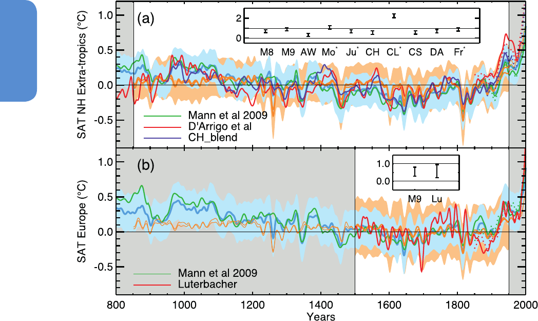
918

Chapter 10 Detection and Attribution of Climate Change: from Global to Regional

uncertainties in forcing or proxy response to it, particularly associated

with volcanism. The discrepancy is reduced when using more strongly

smoothed data or omitting major volcanic eruptions from the analysis.

The level of agreement between ﬁngerprints from multiple models in

response to forcing and reconstructions decreases earlier in time, and

the forced signal is detected only in about half the cases considered

when analysing the period 851 to 1401. This may be partly due to

weaker forcing and larger forcing uncertainty early in the millennium

and partly due to increased uncertainty in reconstructions. Detection

results indicate a contribution by external drivers to the warm con-

ditions in the 11th to 12th century, but cannot explain the warmth

around the 10th century in some of the reconstructions (Figure 10.19).

This detection of a role of external forcing extends work reported in

AR4 back into to the 9th century CE.

Figure 10.19 | The top panel compares the mean annual Northern Hemisphere (NH) surface air temperature from a multi-model ensemble to several NH temperature reconstruc-

tions. These reconstructions are: CH-blend from Hegerl et al. (2007a) in purple, which is a reconstruction of 30°N to 90°N land only (Mann et al., 2009), plotted for the region 30°N

to 90°N land and sea (green) and D’Arrigo et al. (2006) in red, which is a reconstruction of 20°N to 90°N land only. The dotted coloured lines show the corresponding instrumental

data. The multi-model mean for the reconstructed domain is scaled to ﬁt each reconstruction in turn, using a total least squares (TLS) method. The best estimate of the detected

forced signal is shown in orange (as an individual line for each reconstruction; lines overlap closely) with light orange shading indicating the range expected if accounting for

internal variability. The best ﬁt scaling values for each reconstruction are given in the insert as well as the detection results for six other reconstructions (M8; M9 (Mann et al., 2008,

2009); AW (Ammann and Wahl, 2007); Mo (Moberg et al., 2005); Ju (Juckes et al., 2007); CH (Hegerl et al., 2007a); CL (Christiansen and Ljungqvist, 2011) and inverse regressed

onto the instrumental record CS; DA (D’Arrigo et al., 2006); Fr (Frank et al., 2007). An asterisk next to the reconstruction name indicates that the residuals (over the more robustly

reconstructed period 1401–1950) are inconsistent with the internal variability generated by the combined control simulations of all climate models investigated (for details see

Schurer et al., 2013). The ensemble average of a data-assimilation simulation (Goosse et al., 2012b) is plotted in blue, for the region 30°N to 90°N land and sea, with the error

range shown in light blue shading. The bottom panel is similar to the top panel, but showing the European region, following Hegerl et al. (2011a) but using the simulations and

method in Schurer et al. (2013). The detection analysis is performed for the period 1500–1950 for two reconstructions: Luterbacher et al. (2004)(representing the region 35°N to

70°N,25°W to 40°E, “land only, labelled ‘Lu’ in the insert”) shown in red, and Mann et al. (2009) (averaged over the region 25°N to 65°N, 0° to 60°E, land and sea, labelled ‘M9’

in the insert), shown in green. As in the top panel, best ﬁt estimates are shown in dark orange with uncertainty range due to internal variability shown in light orange. The data

assimilation from Goosse et al. (2012a), constrained by the Mann et al. (2009) reconstruction is shown in blue, with error range in light blue. All data are shown with respect to the

mean of the period covered by the white part of the ﬁgure (850–1950 for the NH, 1500–1950 for European mean data).

Detection and attribution studies support results from modelling stud-

ies that infer a strong role of external forcing in the cooling of NH tem-

peratures during the Little Ice Age (LIA; see Chapter 5 and Glossary).

Both model simulations (Jungclaus et al., 2010) and results from detec-

tion and attribution studies (Hegerl et al., 2007a; Schurer et al., 2013)

suggest that a small drop

in GHG concentrations may have contributed

to the cool conditions during the 16th and 17th centuries. Note, how-

ever, that centennial variations of GHG during the late Holocene are

very small relative to their increases since pre-industrial times (Section

6.2.3). The role of solar forcing is less clear except for decreased agree-

ment if using very large solar forcing (e.g., Ammann et al., 2007; Feul-

ner, 2011). Palastanga et al. (2011) demonstrate that neither a slow-

down of the thermohaline circulation nor a persistently negative NAO

alone can explain the reconstructed temperature pattern over Europe

during the periods 1675–1715 and 1790–1820.

919

Detection and Attribution of Climate Change: from Global to Regional Chapter 10

Data assimilation studies support the conclusion that external forcing,

together with internal climate variability, provides a consistent expla-

nation of climate change over the last millennium. Goosse et al. (2010,

2012a, 2012b) select, from a very large ensemble with an EMIC, the

individual simulations that are closest to the spatial reconstructions of

temperature between 30°N and 60°N by Mann et al. (2009) account-

ing for reconstruction uncertainties. The method also varies the exter-

nal forcing within uncertainties, determining a combined realization of

the forced response and internal variability that best matches the data.

Results (Figure 10.19) show that simulations reproduce the target

reconstruction within the uncertainty range, increasing conﬁdence

in the consistency of the reconstruction and the forcing. The results

suggest that long-term circulation anomalies may help to explain the

hemispheric warmth early in the millennium, although results vary

dependent on input parameters of the method.

10.7.1.2 Role of Individual Forcings

Volcanic forcing shows a detectable inﬂuence on large-scale tempera-

ture (see AR4; Chapter 5), and volcanic forcing plays an important role

in explaining past cool episodes, for example, in the late 17th and early

19th centuries (see Chapter 5 and 9; Hegerl et al., 2007b; Jungclaus et

al., 2010; Miller et al., 2012) . Schurer et al. (2013) separately detect the

response to GHG variations between 1400 and 1900 in most NH recon-

structions considered, and that of solar and volcanic forcing combined

in all reconstructions considered.

Even the multi-century perspective makes it difﬁcult to distinguish

century-scale variations in NH temperature due to solar forcing alone

from the response to other forcings, due to the few degrees of freedom

constraining this forcing (see Box 10.2). Hegerl et al. (2003, 2007a)

found solar forcing detectable in some cases. Simulations with higher

than best guess solar forcing may reproduce the warm period around

1000 more closely, but the peak warming occurs about a century ear-

lier in reconstructions than in solar forcing and with it model simu-

lations (Jungclaus et al., 2010; Figure 5.8; Fernández-Donado et al.,

2013). Even if solar forcing were on the high end of estimates for the

last millennium, it would not be able to explain the recent warming

according both to model simulations (Ammann et al., 2007; Tett et al.,

2007; Feulner, 2011) and detection and attribution approaches that

scale the temporal ﬁngerprint of solar forcing to best match the data

(Hegerl et al., 2007a; Schurer et al., 2013; Figure 10.19). Some studies

suggest that particularly for millennial and multi-millenial time scales

orbital forcing may be important globally (Marcott et al., 2013) and for

high-latitude trends (Kaufman et al., 2009) based on a comparison of

the correspondence between long-term Arctic cooling in models and

data though the last millennium up to about 1750 (see also PAGES 2k

Consortium, 2013).

10.7.1.3 Estimates of Internal Climate Variability

The interdecadal and longer-term variability in large-scale temper-

atures in climate model simulations with and without past external

forcing is quite different (Tett et al., 2007; Jungclaus et al., 2010), con-

sistent with the ﬁnding that a large fraction of temperature variance in

the last millennium has been externally driven. The residual variability

in past climate that is not explained by changes in RF provides an

estimate of internal variability for NH mean temperature that is not

directly derived from climate model simulation. This residual variability

is somewhat larger than control simulation variability for some recon-

structions if the comparison is extended to the full period since 850

CE (Schurer et al., 2013), However, when extracting 50- and 60-year

trends from this residual variability, the distribution of these trends is

similar to the multi-model control simulation ensemble used in Schurer

et al. (2013). In all cases considered, the most recent 50-and 60-year

trend from instrumental data is far outside the range of any 50-year

trend in residuals from reconstructions of NH mean temperature of the

past millennium.

10.7.2 Changes of Past Regional Temperature

Several reconstructions of European regional temperature variability

are available (Section 5.5). While Bengtsson et al. (2006) emphasized

the role of internal variability in pre-industrial European climate as

reconstructed by Luterbacher et al. (2004), Hegerl et al. (2011a) ﬁnd

a detectable response to external forcing in summer temperatures in

the period 1500–1900, for winter temperatures during 1500–1950 and

1500–2000; and throughout the record for spring. The ﬁngerprint of

the forced response shows coherent time evolution between models

and reconstructed temperatures over the entire analysed period (com-

pare to annual results in Figure 10.19, using a larger multi-model

ensemble). This suggests that the cold European winter conditions in

the late 17th and early 19th century and the warming in between were

at least partly externally driven.

Data assimilation results focussing on the European sector suggests

that the explanation of forced response combined with internal varia-

bility is self-consistent (Goosse et al., 2012a, Figure 10.19). The assim-

ilated simulations reproduce the warmth of the MCA better than the

forced only simulations do. The response to individual forcings is difﬁ-

cult to distinguish from each other in noisier regional reconstructions.

An epoch analysis of years immediately following strong, largely tropi-

cal, volcanic eruptions shows that European summers show detectable

ﬁngerprints of volcanic response , while winters show a noisy response

of warming in northern Europe and cooling in southern Europe (Hegerl

et al., 2011a). Landrum et al. (2013) suggest similar volcanic responses

for North America, with warming in the north of the continent and

cooling in the south. There is also evidence for a decrease in SSTs fol-

lowing tropical volcanic forcing in tropical reconstructions over the

past 450 years (D’Arrigo et al., 2009). There is also substantial liter-

ature suggesting solar inﬂuences on regional climate reconstructions,

possibly due to circulation changes, for example, changes in Northern

Annular Modes (e.g., Kobashi et al., 2013; see Box 10.2).

10.7.3 Summary: Lessons from the Past

Detection and attribution studies strengthen results from AR4 that

external forcing contributed to past climate variability and change prior

to the 20th century. Ocean–Atmosphere General Circulation Models

(OAGCMs) simulate similar changes on hemispheric and annual scales

as those by simpler models used earlier, and enable detection of

regional and seasonal changes. Results suggest that volcanic forcing

and

GHG forcing in particular are important for explaining past chang-

es in NH temperatures. Results from data assimilation runs conﬁrm

920

Chapter 10 Detection and Attribution of Climate Change: from Global to Regional

that the combination of internal variability and external forcing pro-

vides a consistent explanation of the last millennium and suggest that

changes in circulation may have further contributed to climate anoma-

lies. The role of external forcing extends to regional records, for exam-

ple, European seasonal temperatures. In summary, it is very unlikely

that NH temperature variations from 1400 to 1850 can be explained

by internal variability alone. There is medium conﬁdence that external

forcing contributed to NH temperature variability from 850 to 1400.

There is medium conﬁdence that external forcing (anthropogenic and

natural forcings together) contributed to European temperatures of the

last ﬁve centuries.

10.8 Implications for Climate System

Properties and Projections

Detection and Attribution results can be used to constrain predictions

of future climate change (see Chapters 11 and 12) and key climate

system properties. These properties include: the Equilibrium Climate

Sensitivity (ECS), which determines the long-term equilibrium warming

response to stable atmospheric composition, but not accounting for

vegetation or ice sheet changes (Section 12.5.3; see Box 12.2); the

transient climate response (TCR), which is a measure of the magni-

tude of transient warming while the climate system, particularly the

deep ocean, is not in equilibrium; and the transient climate response to

cumulative CO

emissions (TCRE), which is a measure of the transient

warming response to a given mass of CO

injected into the atmos-

phere, and combines information on both the carbon cycle and cli-

mate response. TCR is more tightly constrained by the observations

of transient warming than ECS. The observational constraints on TCR,

ECS and TCRE assessed here focus on information provided by recent

observed climate change, complementing analysis of feedbacks and

climate modelling information, which are assessed in Chapter 9. The

assessment in this chapter also incorporates observational constraints

based on palaeoclimatic information, building on Chapter 5, and con-

tributes to the overall synthesis assessment in Chapter 12 (Box 12.2).

Because neither ECS nor TCR is directly observed, any inference about

them requires some form of climate model, ranging in complexity from

a simple zero-dimensional energy balance box model to OAGCMs

(Hegerl and Zwiers, 2011). Constraints on estimates of long-term

climate change and equilibrium climate change from recent warm-

ing hinge on the rate at which the ocean has taken up heat (Section

3.2), and by the extent to which recent warming has been reduced by

cooling from aerosol forcing. Therefore, attempts to estimate climate

sensitivity (transient or equilibrium) often also estimate the total aer-

osol forcing and the rate of ocean heat uptake, which are discussed in

Section 10.8.3. The AR4 contained a detailed discussion on estimat-

ing quantities relevant for projections, and included an appendix with

the relevant estimation methods. Here, we build on this assessment,

repeating information and discussion only where necessary to provide

context.

10.8.1 Transient Climate Response

The AR4 discussed for the ﬁrst time estimates of the TCR. TCR was

originally deﬁned as the warming at the time of CO

doubling (i.e.,

after 70 years) in a 1% yr

–1

increasing CO

experiment (see Hegerl et

al., 2007b), but like ECS, it can also be thought of as a generic property

of the climate system that determines the global temperature response

ΔT to any gradual increase in RF, ΔF, taking place over an approximate-

ly 70-year time scale, normalized by the ratio of the forcing change to

the forcing due to doubling CO

, F

2×CO2

: TCR = F

2×CO2

ΔT/ΔF (Frame et

al., 2006; Gregory and Forster, 2008; Held et al., 2010; Otto et al., 2013).

This generic deﬁnition of the TCR has also been called the ‘Transient

Climate Sensitivity’ (Held et al., 2010). TCR is related to ECS and the

global energy budget as follows: ECS = F

2×CO2

/α, where α is the sensi-

tivity parameter representing the net increase in energy ﬂux to space

per degree of warming given all feedbacks operating on these time

scales. Hence, by conservation of energy, ECS = F

2×CO2

ΔT/(ΔF – ΔQ),

where ΔQ is the change in the rate of increase of climate system heat

content in response to the forcing ΔF. On these time scales, deep ocean

heat exchange affects the surface temperature response as if it were

an enhanced radiative damping, introducing a slow, or ‘recalcitrant’,

component of the response which would not be reversed for many

decades even if it were possible to return RF to pre-industrial values

(Held et al., 2010): hence the difﬁculty of placing an upper bound on

ECS from observed surface warming alone (Forest et al., 2002; Frame

et al., 2006). Because ΔQ is always positive at the end of a period of

increasing forcing, before the climate system has re-equilibrated, TCR

is always less than ECS, and since ΔQ is uncertain, TCR is generally

better constrained by observations of recent climate change than ECS.

Because TCR focuses on the short- and medium-term response, con-

straining TCR with observations is a key step in narrowing estimates of

future global temperature change in the relatively short term and under

scenarios where forcing continues to increase or peaks and declines

(Frame et al., 2006). After stabilization, the ECS eventually becomes the

relevant climate system property. Based on observational constraints

alone, the AR4 concluded that TCR is very likely to be larger than 1°C

and very unlikely to be greater than 3.5°C (Hegerl et al., 2007b). This

supported the overall assessment that the transient climate response is

very unlikely greater than 3°C and very likely greater than 1°C (Meehl

et al., 2007a). New estimates of the TCR are now available.

Scaling factors derived from detection and attribution studies (see Sec-

tion 10.2) express how model responses to GHGs and aerosols need to

be scaled to match the observations over the historical period. These

scaled responses were used in AR4 to provide probabilistic projections

of both TCR and future changes in global temperature in response to

these forcings under various scenarios (Allen et al., 2000; Stott and Ket-

tleborough, 2002; Stott et al., 2006, 2008b; Kettleborough et al., 2007;

Meehl et al., 2007b; Stott and Forest, 2007). Allen et al. (2000), Frame

et al. (2006) and Kettleborough et al. (2007) demonstrate a near linear

relationship between 20th century warming, TCR and warming by the

mid-21st century as parameters are varied in Energy Balance Models,

justifying this approach. Forster et al. (2013 ) show how the ratio ΔT/

ΔF does depend on the forcing history, with very rapid increases in

forcing giving lower values: hence any inference from past attributable

warming to future warming or TCR depends on a model (which may be

simple or complex, but ideally physically based) to relate these quanti-

ties. Such inferences also depend on forcing estimates and projections.

Recent revisions to RF (see Chapter 8) suggest higher net anthropo-

genic forcing over the 20th century, and hence a smaller estimated

921

Detection and Attribution of Climate Change: from Global to Regional Chapter 10

TCR. Stott et al. (2008b) demonstrated that optimal detection analy-

sis of 20th century temperature changes (using HadCM3) are able to

exclude the very high and low temperature responses to aerosol forc-

ing. Consequently, projected 21st century warming may be more close-

ly constrained than if the full range of aerosol forcings is used (Andreae

et al., 2005). Stott and Forest (2007) demonstrate that projections

obtained from such an approach are similar to those obtained by con-

straining EMIC parameters from observations. Stott et al. (2011), using

HadGEM2-ES, and Gillett et al. (2012), using CanESM2, both show that

the inclusion of observations between 2000 and 2010 in such an anal-

ysis reduces the uncertainties in projected warming in the 21st century,

and tends to constrain the maximum projected warming to below that

projected using data to 2000 only (Stott et al, 2006). Such an improve-

ment is consistent with prior expectations of how additional data will

narrow uncertainties (Stott and Kettleborough, 2002).

TCR estimates have been derived using a variety of methods (Figure

10.20a). Knutti and Tomassini (2008) compare EMIC simulations with

20th century surface and ocean temperatures to derive a probability

density function for TCR skewed slightly towards lower values with a

5 to 95% range of 1.1°C to 2.3°C. Libardoni and Forest (2011) take a

similar approach with a different EMIC and include atmospheric data

and, under a variety of assumptions, obtain 5 to 95%ranges for TCR

spanning 0.9°C to 2.4°C. Updating this study to include data to 2004

gives results that are essentially unchanged. Using a single model and

observations from 1851 to 2010 Gillett et al. (2012) derive a 5 to 95%

range of 1.3°C to 1.8°C and using a single model, but using multiple

sets of observations and analysis periods ending in 2010 and begin-

ning in 1910 or earlier, Stott et al. (2011) derive 5 to 95% ranges that

were generally between 1°C and 3°C. Both Stott et al. (2011) and Gil-

lett et al. (2012) ﬁnd that the inclusion of data between 2000 and

2010 helps to constrain the upper bound of TCR. Gillett et al. (2012)

ﬁnd that the inclusion of data prior to 1900 also helps to constrain

TCR, though Stott et al. (2011) do not. Gillett et al. (2013 ) account for

a broader range of model and observational uncertainties, in particular

addressing the efﬁcacy of non-CO

gases, and ﬁnd a range of 0.9°C to

2.3°C. Several of the estimates of TCR that were cited by Hegerl et al.

(2007b) may have underestimated non-CO

efﬁcacies relative to the

more recent estimates in Forster et al. (2007). Because observational-

ly constrained estimates of TCR are based on the ratio between past

attributable warming and past forcing, this could account for a high

bias in some of the inputs used for the AR4 TCR estimate.

Held et al. (2010) show that a two-box model originally proposed by

Gregory (2000), distinguishing the ‘fast’ and ‘recalcitrant’ responses,

ﬁts both historical simulations and instantaneous doubled CO

sim-

ulations of the GFDL coupled model CM2.1. The fast response has a

relaxation time of 3 to 5 years, and the historical simulation is almost

completely described by this fast component of warming. Padilla et al.

(2011) use this simple model to derive an observationally constrained

estimate of the TCR of 1.3°C to 2.6°C. Schwartz (2012) uses this two-

time scale formulation to obtain TCR estimates ranging from 0.9°C to

1.9°C, the lower values arising from higher estimates of forcing over

the 20th century. Otto et al. (2013) update the analysis of Gregory et

al. (2002) and Gregory and Forster (2008) using forcing estimates from

Forster et al. (2013 ) to obtain a 5 to 95% range for TCR of 0.9°C to

2.0°C comparing the decade 2000–2009 with the period 1860–1879.

They note, however, the danger of overinterpreting a single, possibly

anomalous, decade, and report a larger TCR range of 0.7°C to 2.5°C

replacing the 2000s with the 40 years 1970–2009.

Tung et al. (2008) examine the response to the 11-year solar cycle using

discriminant analysis, and ﬁnd a high range for TCR: >2.5°C to 3.6°C

However, this estimate may be affected by different mechanisms by

which solar forcing affects climate (see Box 10.2). The authors attempt

to minimize possible aliasing with the response to other forcings in

the 20th century and with internal climate variability, although some

inﬂuence by them cannot be ruled out.

Rogelj et al. (2012) take a somewhat different approach, using a simple

climate model to match the distribution of TCR to observational con-

straints and a consensus distribution of ECS (which will itself have

been informed by recent climate change), following Meinshausen et

al. (2009). Harris et al. (2013) estimate a distribution for TCR based on

a large sample of emulated GCM equilibrium responses, constrained

by multiannual mean observations of recent climate and adjusted to

account for additional uncertainty associated with model structural

deﬁciencies (Sexton et al., 2012). The equilibrium responses are scaled

by global temperature changes associated with the sampled model

variants, reweighting the projections based on the likelihood that they

correctly replicate observed historical changes in surface temperature,

to predict the TCR distribution. Both of these studies represent a com-

bination of multiple lines of evidence, although still strongly informed

by recent observed climate change, and hence are assessed here for

completeness.

Based on this evidence, including the new 21st century observations

that were not yet available to AR4, we conclude that, on the basis of

constraints provided by recent observed climate change, TCR is likely to

lie in the range 1°C to 2.5°C and extremely unlikely to be greater than

3°C. This range for TCR is smaller than given at the time of AR4, due

to the stronger observational constraints and the wider range of stud-

ies now available. Our greater conﬁdence in excluding high values of

TCR arises primarily from higher and more conﬁdent estimates of past

forcing: estimates of TCR are not strongly dependent on observations

of ocean heat uptake.

10.8.2 Constraints on Long-Term Climate Change and the

Equilibrium Climate Sensitivity

The equilibrium climate sensitivity (ECS) is deﬁned as the warming in

response to a sustained doubling of carbon dioxide in the atmosphere

relative to pre-industrial levels (see AR4). The equilibrium to which

the ECS refers to is generally assumed to be an equilibrium involving

the ocean–atmosphere system, which does not include Earth system

feedbacks such as long-term melting of ice sheets and ice caps, dust

forcing or vegetation changes (see Chapter 5 and Section 12.5.3). The

ECS cannot be directly deduced from transient warming attributable to

GHGs, or from TCR, as the role of ocean heat uptake has to be taken

into account (see Forest et al., 2000; Frame et al., 2005; Knutti and

Hegerl, 2008). Estimating the ECS generally relies on the paradigm of

a comparison of observed change with results from a physically based

climate model, sometimes a very simple one, given uncertainty in the

model, data, RF and due to internal variability.

922

Chapter 10 Detection and Attribution of Climate Change: from Global to Regional

For example, estimates can be based on the simple box model intro-

duced in Section 10.8.1, ECS = F

2×CO2

ΔT/(ΔF – ΔQ). Simple energy

balance calculations rely on a very limited representation of climate

response time scales, and cannot account for nonlinearities in the cli-

mate system that may lead to changes in feedbacks for different forc-

ings (see Chapter 9). Alternative approaches are estimates that use

climate model ensembles with varying parameters that evaluate the

ECS of individual models and then infer the probability density function

(PDF) for the ECS from the model–data agreement or by using optimi-

zation methods (Tanaka et al., 2009).

As discussed in the AR4, the probabilistic estimates available in the

literature for climate system parameters, such as ECS and TCR have all

been based, implicitly or explicitly, on adopting a Bayesian approach

and therefore, even if it is not explicitly stated, involve using some

kind of prior information. The shape of the prior has been derived from

expert judgement in some studies, observational or experimental evi-

dence in others or from the distribution of the sample of models avail-

able. In all cases the constraint by data, for example, from transient

warming, or observations related to feedbacks is fairly weak on the

upper tail of ECS (e.g., Frame et al., 2005). Therefore, results are sensi-

tive to the prior assumptions (Tomassini et al., 2007; Knutti and Hegerl,

2008; Sanso and Forest, 2009; Aldrin et al., 2012). When the prior distri-

bution fails to taper off for high sensitivities, as is the case for uniform

priors (Frame et al., 2005), this leads to long tails (Frame et al., 2005;

Annan and Hargreaves, 2011; Lewis, 2013). Uniform priors have been

criticized (e.g., Annan and Hargreaves, 2011; Pueyo, 2012; Lewis, 2013)

since results assuming a uniform prior in ECS translates instead into a

strongly structured prior on climate feedback parameter and vice versa

(Frame et al., 2005; Pueyo, 2012). Objective Bayesian analyses attempt

to avoid this paradox by using a prior distribution that is invariant

to parameter transforms and rescaling, for example, a Jeffreys prior

(Lewis, 2013). Estimated probability densities based on priors that are

strongly non-uniform in the vicinity of the best ﬁt to the data, as is typi-

cally the case for the Jeffreys prior in this instance, can peak at values

very different from the location of the best ﬁt, and hence need to be

interpreted carefully. To what extent results are sensitive to priors can

be evaluated by using different priors, and this has been done more

consistently in studies than at the time of AR4 (see Figure 10.20b) and

is assessed where available, illustrated in Figure 10.20. Results will also

be sensitive to the extent to which uncertainties in forcing (Tanaka et

al., 2009), models and observations and internal climate variability are

taken into account, and can be acutely sensitive to relatively arbitrary

choices of observation period, choice of truncation in estimated covar-

iance matrices and so forth (Lewis, 2013), illustrating the importance

of sensitivity studies. Analyses that make a more complete effort to

estimate all uncertainties affecting the model–data comparison lead to

more trustworthy results, but end up with larger uncertainties (Knutti

and Hegerl, 2008).

The detection and attribution chapter in AR4 (Hegerl et al., 2007b) con-

cluded that ‘Estimates based on observational constraints indicate that

it is very likely that the equilibrium climate sensitivity is larger than 1.5°C

with a most likely value between 2°C and 3°C’. The following sections

discuss evidence since AR4 from several lines of evidence, followed by

an overall assessment of ECS based on observed climate changes, and a

subset of available new estimates is shown in Figure 10.20b.

10.8.2.1 Estimates from Recent Temperature Change

As estimates of ECS based on recent temperature change can only

sample atmospheric feedbacks that occur with presently evolving cli-

mate change, they provide information on the ‘effective climate sen-

sitivity’ (e.g., Forest et al., 2008). As discussed in AR4, analyses based

on global scale data ﬁnd that within data uncertainties, a strong aer-

osol forcing or a large ocean heat uptake might have masked a strong

greenhouse warming (see, e.g., Forest et al., 2002; Frame et al., 2005;

Stern, 2006; Roe and Baker, 2007; Hannart et al., 2009; Urban and

Keller, 2009; Church et al., 2011). This is consistent with the ﬁnding that

a set of models with a large range of ECS and aerosol forcing could

be consistent with the observed warming (Kiehl, 2007). Consequent-

ly, such analyses ﬁnd that constraints on aerosol forcing are essen-

tial to provide tighter constraints on future warming (Tanaka et al.,

2009; Schwartz et al., 2010). Aldrin et al. (2012) analyse the observed

record from 1850 to 2007 for hemispheric means of surface temper-

ature, and upper 700 m ocean heat content since 1955. The authors

use a simple climate model and a Markov Chain Monte Carlo Bayesian

technique for analysis. The authors ﬁnd a quite narrow range of ECS,

which narrows further if using a uniform prior in 1/ECS rather than

ECS (Figure 10.20). If observations are updated to 2010 and forcing

estimates including further indirect aerosol effects are used (following

Skeie et al., 2011), this yields a reduced upper tail (see Figure 10.20b,

dash dotted). However, this estimate involves a rather simple model for

internal variability, hence may underestimate uncertainties. Olson et

al. (2012) use similar global scale constraints and surface temperature

to 2006, and ocean data to 2003 and arrive at a wide range if using a

uniform prior in ECS, and a quite well constrained range if using a prior

derived from current mean climate and Last Glacial Maximum (LGM)

constraints (see Figure 10.20b). Some of the differences between Olson

et al. (2012) and Aldrin et al. (2012) may be due to structural differences

in the model used (Aldrin et al. use a simple EBM while Olson use the

UVIC EMIC), some due to different statistical methods and some due to

use of global rather than hemispheric temperatures in the latter work.

An approach based on regressing forcing histories used in 20th century

simulations on observed surface temperatures (Schwartz, 2012) esti-

mates ranges of ECS that encompass the AR4 ranges if accounting for

data uncertainty (Figure 10.20). Otto et al. (2013) updated the Greg-

ory et al. (2002) global energy balance analysis (see equation above),

using temperature and ocean heat content data to 2009 and estimates

of RF that are approximately consistent with estimates from Chapters

7 and 8, and ocean heat uptake estimates that are consistent with

Chapter 3 and ﬁnd that inclusion of recent deep ocean heat uptake and

temperature data considerably narrow estimates of ECS compared to

results using data to the less recent past.

Estimates of ECS and TCR that make use of both spatial and tempo-

ral information, or separate the GHG attributable warming using ﬁn-

gerprint methods, can yield tighter estimates (e.g., Frame et al., 2005;

Forest et al., 2008; Libardoni and Forest, 2011). The resulting GHG

attributable warming tends to be reasonably robust to uncertainties in

aerosol forcing (Section 10.3.1.1.3). Forest et al. (2008) have updated

their earlier study using a newer version of the MIT model and ﬁve

different surface temperature data sets (Libardoni and Forest, 2011).

Correction of statistical errors in estimation procedure pointed out by

Lewis (see Lewis, 2013) changes their result only slightly (Libardoni

923

Detection and Attribution of Climate Change: from Global to Regional Chapter 10

and Forest, 2013). The overarching 5 to 95% range of effective cli-

mate sensitivity widens to 1.2°C to 5.3°C when all ﬁve data sets are

used, and constraints on effective ocean diffusivity become very weak

(Forest et al., 2008). Uncertainties would likely further increase if esti-

mates of forcing uncertainty, for example, due to natural forcings, are

also included (Forest et al., 2006). Lewis (2013) reanalysed the data

used in Forest et al. (2006) using an objective Bayesian method (see

discussion at top of section). The author ﬁnds that use of a Jeffreys

prior narrows the upper tail considerably, to 3.6°C for the 95th percen-

tile. When revising the method, omitting upper air data, and adding 6

more years of data a much reduced 5 to 95% range of 1.2°C to 2.2°C

results (see Figure 10.20), similar to estimates by Ring et al. (2012)

using data to 2008. Lewis’s upper limit extends to 3.0°C if accounting

for forcing and surface temperature uncertainty (Lewis, 2013). Lewis

(2013) also reports a range of 1.1°C to 2.9°C using his revised diag-

nostics and the Forest et al. (2006) statistical method, whereas adding

9 more years to the Libardoni and Forest (2013) corrected diagnostic

(after Libardoni and Forest, 2011; Figure 10.20; using an expert prior

in both cases), does not change results much (Figure 10.20b). The dif-

ferences between results reported in Forest et al. (2008); Libardoni and

Forest (2011); Lewis (2013); Libardoni and Forest (2013) are still not

fully understood, but appear to be due to a combination of sensitivity

of results to the choice of analysis period as well as differences in diag-

nostics and statistical approach.

In summary, analyses that use the most recent decade ﬁnd a tighten-

ing of the range of ECS based on a combination of recent heat uptake

and surface temperature data. Results consistently give low probability

to ECS values under 1.0°C (Figure 10.20). The mode of the PDFs varies

considerably with period considered as expected from the inﬂuence of

internal variability on the single realization of observed climate change.

Estimates including the most recent data tend to have reduced upper

tails (Libardoni and Forest, 2011; Aldrin et al., 2012 and update; Ring

et al., 2012 and update cf. Figure 10.20; Lewis, 2013; Otto et al., 2013),

although further uncertainty in statistical assumptions and structural

uncertainties in simple models used, as well as neglected uncertainties,

for example, in forcings, increase assessed uncertainty.

10.8.2.2 Estimates Based on Top of the Atmosphere Radiative

Balance

With the satellite era, measurements are now long enough to allow

direct estimates of variations in the energy budget of the planet,

although the measurements are not sufﬁciently accurate to determine

absolute top of the atmosphere (TOA) ﬂuxes or trends (see Section 2.3

and Box 13.1). Using a simple energy balance relationship between

net energy ﬂow towards the Earth, net forcing and a climate feedback

parameter and the satellite measurements Murphy et al. (2009) made

direct estimates of the climate feedback parameter as the regression

coefﬁcient of radiative response against GMST. The feedback parame-

ter in turn is inversely proportional to the ECS (see above, also Forster

and Gregory, 2006). Such regression based estimates are, however,

subject to uncertainties (see Section 7.2.5.7; see also, Gregory and For-

ster, 2008; Murphy and Forster, 2010). Lindzen and Choi (2009) used

data from the radiative budget and simple energy balance models over

the tropics to investigate feedbacks in climate models. Their result

suggests that climate models overestimate the outgoing shortwave

radiation compared to Earth Radiation Budget Experiment (ERBE) data,

but this result was found unreliable owing to use of a limited sample

of periods and of a domain limited to low latitudes (Murphy and For-

ster, 2010). Lindzen and Choi (2011) address some of these criticisms

(Chung et al., 2010; Trenberth et al., 2010), but the results remains

uncertain. For example, the lag-lead relationship between TOA balance

and SST (Lindzen and Choi, 2011) is replicated by Atmospheric Model

Intercomparison Project (AMIP) simulations where SST cannot respond

(Dessler, 2011). Hence, as discussed in Section 7.2.5.7, the inﬂuence of

internal temperature variations on short time scales seriously affects

such estimates of feedbacks. In addition, the energy budget changes

that are used to derive feedbacks are also affected by RF, which Lin-

dzen and Choi (2009) do not account for. Murphy and Forster (2010)

further question if estimates of the feedback parameter are suitable

to estimate the ECS, as multiple time scales are involved in feedbacks

that contribute to climate sensitivity (Knutti and Hegerl, 2008; Dessler,

2010). Lin et al. (2010a) use data over the 20th century combined with

an estimate of present TOA imbalance based on modelling (Hansen et

al., 2005a) to estimate the energy budget of the planet and give a best

estimate of ECS of 3.1°C, but do not attempt to estimate a distribution

that accounts fully for uncertainties. In conclusion, measurement and

methodological uncertainties in estimates of the feedback parameter

and the ECS from short-term variations in the satellite period preclude

strong constraints on ECS. When accounting for these uncertainties,

estimates of ECS based on the TOA radiation budget appear consistent

with those from other lines of evidence within large uncertainties (e.g.,

Forster and Gregory, 2006; Figure 10.20b).

10.8.2.3 Estimates Based on Response to Volcanic Forcing or

Internal Variability

Some analyses used in AR4 were based on the well observed forcing

and responses to major volcanic eruptions during the 20th century.

The constraint is fairly weak because the peak response to short-term

volcanic forcing depends nonlinearly on ECS (Wigley et al., 2005; Boer

et al., 2007). Recently, Bender et al. (2010) re-evaluated the constraint

and found a close relationship in 9 out of 10 AR4 models between the

shortwave TOA imbalance, the simulated response to the eruption of

Mt Pinatubo and the ECS. Applying the constraint from observations

suggests a range of ECS of 1.7°C to 4.1°C. This range for ECS is subject

to observational uncertainty and uncertainty due to internal climate

variability, and is derived from a limited sample of models. Schwartz

(2007) tried to relate the ECS to the strength of natural variability using

the ﬂuctuation dissipation theorem but studies suggest that the obser-

vations are too short to support a well constrained and reliable esti-

mate and would yield an underestimate of sensitivity (Kirk-Davidoff,

2009); and that assuming single time scales is too simplistic for the

climate system (Knutti and Hegerl, 2008) . Thus, credible estimates of

ECS from the response to natural and internal variability do not disa-

gree with other estimates, but at present cannot provide more reliable

estimates of ECS.

10.8.2.4 Paleoclimatic Evidence

Palaeoclimatic evidence is promising for estimating ECS (Edwards

et al., 2007). This section reports on probabilistic estimates of ECS

derived from paleoclimatic data by drawing on Chapter 5 information

924

Chapter 10 Detection and Attribution of Climate Change: from Global to Regional

on forcing and temperature changes. For periods of past climate, which

were close to radiative balance or when climate was changing slowly,

for example, the LGM, radiative imbalance and with it ocean heat

uptake is less important than for the present (Sections 5.3.3.1 and

5.3.3.2). Treating the RF due to ice sheets, dust and CO

as forcings

rather than feedbacks implies that the corresponding RF contributions

are associated with considerable uncertainties (see Section 5.2.2.3).

Koehler et al. (2010) used an estimate of LGM cooling along with its

uncertainties together with estimates of LGM RF and its uncertainty to

derive an overall estimate of climate sensitivity. This method accounts

for the effect of changes in feedbacks for this very different climatic

state using published estimates of changes in feedback factors (see

Section 5.3.3.2; Hargreaves et al., 2007; Otto-Bliesner et al., 2009). The

authors ﬁnd a best estimate of 2.4°C and a 5 to 95% range of ECS

from 1.4°C to 5.2°C, with sensitivities beyond 6°C difﬁcult to reconcile

with the data. In contrast, Chylek and Lohmann (2008b) estimate the

ECS to be 1.3°C to 2.3°C based on data for the transition from the

LGM to the Holocene. However, the true uncertainties are likely larger

due to uncertainties in relating local proxies to large-scale temperature

change observed over a limited time (Ganopolski and von Deimling,

2008; Hargreaves and Annan, 2009). The authors also use an aerosol

RF estimate that may be high (see response by Chylek and Lohmann,

2008a; Ganopolski and von Deimling, 2008).

At the time of the AR4, several studies were assessed in which param-

eters in climate models had been perturbed systematically in order to

estimate ECS, and further studies have been published since, some

making use of expanded data for LGM climate change (see Section

5.3.3.2, Table 5.3). Sometimes substantial differences between esti-

mates based on similar data reﬂect not only differences in assumptions

on forcing and use of data, but also structural model uncertainties, for

example, in how feedbacks change between different climatic states

(e.g., Schneider von Deimling et al., 2006; Hargreaves et al., 2007; (see

also Otto-Bliesner et al., 2009). Holden et al. (2010) analysed which

versions of the EMIC Genie are consistent with LGM tropical SSTs and

ﬁnd a 90% range of 2.0°C to 5.0°C. Recently, new data synthesis prod-

ucts have become available for assessment with climate model simu-

lations of the LGM which together with further data cover much more

of the LGM ocean and land areas, although there are still substantial

gaps and substantial data uncertainty (Section 5.3.3). An analysis of

the recent SST and land temperature reconstructions for the LGM com-

pared to simulations with an EMIC suggests a 90% range of 1.4°C to

2.8°C for ECS, with SST data providing a narrower range and lower

values than land data only (see Figure 10.20; Schmittner et al., 2011).

However, structural model uncertainty as well as data uncertainty may

increase this range substantially (Fyke and Eby, 2012; Schmittner et

al., 2012). Hargreaves et al. (2012) derived a relationship between ECS

and LGM response for seven model simulations from PMIP2 simula-

tions and found a linear relationship between tropical cooling and ECS

(see Section 5.3.3.2) which has been used to derive an estimate of

ECS (Figure 10.20); and has been updated using PMIP3 simulations

(Section 5.3.3.2). However, uncertainties remain as the relationship is

dependent on the ensemble of models used.

Estimates of ECS from other, more distant paleoclimate periods (e.g.,

Royer et al., 2007; Royer, 2008; Pagani et al., 2009; Lunt et al., 2010)

are difﬁcult to directly compare, as climatic conditions were very

different from today and as climate sensitivity can be state depend-

ent, as discussed above. Also, the response on very long time scales is

determined by the Earth System Sensitivity, which includes very slow

feedbacks by ice sheets and vegetation (see Section 12.5.3). Paleosens

Members (2012) reanalysed the relationship between RF and temper-

ature response from paleoclimatic studies, considering Earth system

feedbacks as forcings in order to derive an estimate of ECS that is limit-

ed to atmospheric feecbacks (sometimes referred to as Charney sensi-

tivity and directly comparable to ECS), and ﬁnd that resulting estimates

are reasonably consistent over the past 65 million years (see detailed

discussion in Section 5.3.1). They estimate a 95% range of 1.1°C to

7.0°C, largely based on the past 800,000 years. However, uncertain-

ties in paleoclimate estimates of ECS are likely to be larger than from

the instrumental record, for example, due to changes in feedbacks

between different climatic states. In conclusion, estimates of ECS have

continued to emerge from palaeoclimatic periods that indicate that

ECS is very likely less than 6°C and very likely greater than 1.0°C (see

Section 5.3.3).

10.8.2.5 Combining Evidence and Overall Assessment

Most studies ﬁnd a lower 5% limit for ECS between 1°C and 2°C (Figure

10.20). The combined evidence thus indicates that the net feedbacks to

RF are signiﬁcantly positive. At present, there is no credible individual

line of evidence that yields very high or very low climate sensitivity as

best estimate. Some recent studies suggest a low climate sensitivity

(Chylek et al., 2007; Schwartz et al., 2007; Lindzen and Choi, 2009).

However, these are based on problematic assumptions, for example,

about the climate’s response time, the cause of climate ﬂuctuations,

or neglect uncertainty in forcing, observations and internal variability

(as discussed in Foster et al., 2008; Knutti and Hegerl, 2008; Murphy

and Forster, 2010). In some cases the estimates of the ECS have been

refuted by testing the method of estimation with a climate model of

known sensitivity (e.g., Kirk-Davidoff, 2009).

Several authors (Annan and Hargreaves, 2006; Hegerl et al., 2006;

Annan and Hargreaves, 2010) had proposed combining estimates

of climate sensitivity from different lines of evidence by the time of

AR4; these and recent work is shown in the panel ‘combined’ in Figure

10.20. Aldrin et al. (2012) combined the Hegerl et al. (2006) estimate

based on the last millennium with their estimate based on the 20th

century; and Olson et al. (2012) combined weak constraints from cli-

matology and the LGM in their prior, updated by data on temperature

changes. This approach is robust only if the lines of evidence used are

truly independent. The latter is hard to evaluate when using prior distri-

butions based on expert knowledge (e.g., Libardoni and Forest, 2011).

If lines of evidence are not independent, overly conﬁdent assessments

of equilibrium climate sensitivity may result (Henriksson et al., 2010;

Annan and Hargreaves, 2011).

In conclusion, estimates of the Equilibrium Climate Sensitivity (ECS)

based on multiple and partly independent lines of evidence from

observed climate change, including estimates using longer records of

surface temperature change and new palaeoclimatic evidence, indi-

cate that there is high conﬁdence that ECS is extremely unlikely less

than 1°C and medium conﬁdence that the ECS is likely between 1.5°C

and 4.5°C and very unlikely greater than 6°C. They complement the

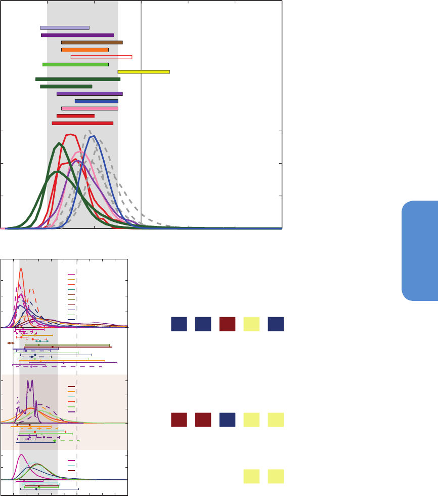
925

Detection and Attribution of Climate Change: from Global to Regional Chapter 10

012 3 4 5 6

0.5

1.5

Dashed lines AR4 studies

Transient Climate Response (°C)

Probability / Relative Frequency (°C

-1

)Probability / Relative Frequency (°C

-1

)

Knutti & Tomassini (2008) uniform ECS prior

Knutti & Tomassini (2008) expert ECS prior

Meinshausen et al (2009)

Harris et al (2013)

Rogelj et al (2012)

Otto et al (2013) −− 1970−2009 budget

Otto et al (2013) −− 2000−2009 budget

Tung et al (2008)

Gillett et al (2013)

Stott & Forest (2007)

Gregory & Forster (2008)

Padilla et al (2011)

Libardoni & Forest (2011)

Schwartz (2012)

0 1 2 3 4

8 9 10

Equilibrium Climate Sensitivity

(°C)

0.0

0.4

0.8

1.2

Aldrinetal. (2012)

Bender et al.(2010)

Lewis(2013)

Linetal. (2010)

Lindzen&Choi (2011)

Murphy et al.(2009)

Olsonetal. (2012)

Otto et al.(2013)

Schwartz(2012)

Tomassini et al.(2007)

0.0

0.4

0.8

1.2

Chylek&Lohmann(2008)

Hargreaves et al.(2012)

Holden et al.(2010)

ohleretal. (2010)

Palaeosens (2012)

Schmittner et al.(2012)

0.0

0.4

0.8

Aldrinetal. (2012)

Libardoni&Forest(2013)

Olsonetal. (2012)

Instrumental

Similar climate

base state

Similar feedbacks

Close to equilibrium

Uncertainties accounted

for/known

Overall level of

scientiﬁc understanding

Palaeoclimate

Combination

Figure 10.20 | (a) Examples of distributions of the transient climate response (TCR, top) and the equilibrium climate sensitivity (ECS, bottom) estimated from observational con-

straints. Probability density functions (PDFs), and ranges (5 to 95%) for the TCR estimated by different studies (see text). The grey shaded range marks the very likely range of 1°C to

2.5°C for TCR and the grey solid line represents the extremely unlikely <3°C upper bound as assessed in this section. Representative distributions from AR4 shown as dashed lines

and open bar. (b) Estimates of ECS are compared to overall assessed likely range (solid grey), with solid line at 1°C and a dashed line at 6°C. The ﬁgure compares some selected

old estimates used in AR4 (no labels, thin lines; for references see Supplementary Material) with new estimates available since AR4 (labelled, thicker lines). Distributions are shown

where available, together with 5 to 95% ranges and median values (circles). Ranges that are assessed as being incomplete are marked by arrows; note that in contrast to the other

estimates Schwartz (2012), shows a sampling range and Chylek and Lohmann a 95% range. Estimates are based on changes over the instrumental period (top row); and changes

from palaeoclimatic data (2nd row). Studies that combine multiple lines of evidence are shown in the bottom panel. The boxes on the right-hand side indicate limitations and

strengths of each line of evidence, for example, if a period has a similar climatic base state, if feedbacks are similar to those operating under CO

doubling, if the observed change

is close to equilibrium, if, between all lines of evidence plotted, uncertainty is accounted for relatively completely, and summarizes the level of scientiﬁc understanding of this line of

evidence overall. A blue box indicates an overall line of evidence that is well understood, has small uncertainty, or many studies and overall high conﬁdence. Pale yellow indicates

medium, and dark red low, conﬁdence (i.e., poorly understood,very few studies, poor agreement, unknown limitations, after Knutti and Hegerl, 2008). Where available, results

are shown using several different prior distributions; for example for Aldrin et al. (2012) solid shows the result using a uniform prior in ECS, which is shown as updated to 2010

in dash-dots; dashed: uniform prior in 1/ECS; and in bottom panel, result combining with Hegerl et al. (2006) prior, For Lewis (2013), dashed shows results using the Forest et al.

(2006) diagnostic and an objective Bayesian prior, solid a revised diagnostic. For Otto et al. (2013), solid is an estimate using change to 1979–2009, dashed using the change to

2000–2009. Palaeoclimate: Hargreaves et al. (2012) is shown in solid, with dashed showing an update based on PMIP3 simulations (see Chapter 5); For Schmittner et al. (2011),

solid is land-and-ocean, dashed land-only, and dash-dotted is ocean-only diagnostic.

926

Chapter 10 Detection and Attribution of Climate Change: from Global to Regional

evaluation in Chapter 9 and support the overall assessment in Chapter

12 that concludes between all lines of evidence with high conﬁdence

that ECS is likely in the range 1.5°C to 4.5°C. Earth system feedbacks

can lead to different, probably larger, warming than indicated by ECS

on very long time scales.

10.8.3 Consequences for Aerosol Forcing and Ocean

Heat Uptake

Some estimates of ECS also yield estimates of aerosol forcing that are

consistent with observational records, which we brieﬂy mention here.

Note that the estimate will reﬂect any forcings with a time or time–

space pattern resembling aerosol forcing that is not explicitly includ-

ed in the overall estimate (see discussion in Olson et al., 2012), for

example, BC on snow; and should hence be interpreted as an estimate

of aerosol plus neglected forcings. Estimates will also vary with the

method applied and diagnostics used (e.g., analyses including spatial

information will yield stronger results). Murphy et al. (2009) use cor-

relations between surface temperature and outgoing shortwave and

longwave ﬂux over the satellite period to estimate how much of the

total recent forcing has been reduced by aerosol total reﬂection, which

they estimate as –1.1 ± 0.4 W m

–2

from 1970 to 2000 (1 standard devi-

ation), while Libardoni and Forest (2011), see also Forest et al. (2008),

based on the 20th century, ﬁnd somewhat lower estimates, namely a

90% bound of –0.83 to –0.19 W m

–2

for the 1980s relative to preindus-

trial. Lewis (2013), using similar diagnostics but an objective Bayesi-

an method, estimates a total aerosol forcing of about –0.6 to –0.1W

–2

or –0.6 to 0.0 W m

–2

dependent on diagnostic used. The range of

the aerosol forcing estimates that are based on the observed climate

change are in-line with the expert judgement of the effective RF by

aerosol radiation and aerosol cloud interactions combined (ERFaci+ari;

Chapter 7) of –0.9 W m

–2

with a range from –1.9 to –0.1 W m

–2

that

has been guided by climate models that include aerosol effects on

mixed-phase and convective clouds in addition to liquid clouds, satel-

lite studies and models that allow cloud-scale responses (see Section

7.5.2).

Several estimates of ECS also estimate a parameter that describe the

efﬁciency with which the ocean takes up heat, e.g., effective global

vertical ocean diffusivity (e.g., Tomassini et al., 2007; Forest et al., 2008;

Olson et al., 2012; Lewis, 2013). Forest and Reynolds (2008) ﬁnd that

the effective global ocean diffusivity K

in many of the CMIP3 models

lies above the median value based on observational constraints, result-

ing in a positive bias in their ocean heat uptake. Lewis (2013) similarly

ﬁnds better agreement for small values of effective ocean diffusivity.

However, such a ﬁnding was very sensitive to data sets used for sur-

face temperature (Libardoni and Forest, 2011) and ocean data (Sokolov

et al., 2010), is somewhat sensitive to the diagnostic applied (Lewis,

2013), and limited by difﬁculties observing heat uptake in the deep

ocean (see, e.g., Chapters 3 and 13). Olson et al. (2012) and Tomassini

et al. (2007) ﬁnd that data over the historical period provide only a

weak constraint on background ocean effective diffusivity. Compari-

son of the vertical proﬁles of temperature and of historical warming

in models and observations suggests that the ocean heat uptake efﬁ-

ciency may be typically too large (Kuhlbrodt and Gregory, 2012; Sec-

tion 13.4.1; see also Sections 9.4.2, 10.4.1, 10.4.3). If effective diffu-

sivity were high in models this might lead to a tendency to bias ocean

warming high relative to surface warming; but this uncertainty makes

only a small contribution to uncertainty in TCR (Knutti and Tomassini,

2008; Kuhlbrodt and Gregory, 2012; see Section 13.4.1). Nonetheless,

ocean thermal expansion and heat content change simulated in CMIP5

models show relatively good agreement with observations, although

this might also be due to a compensation between ocean heat uptake

efﬁciency and atmospheric feedbacks (Kuhlbrodt and Gregory, 2012).

In summary, constraints on effective ocean diffusivity are presently not

conclusive.

10.8.4 Earth System Properties

A number of papers have found the global warming response to CO

emissions to be determined primarily by total cumulative emissions of

, irrespective of the timing of those emissions over a broad range

of scenarios (Allen et al., 2009; Matthews et al., 2009; Zickfeld et al.,

2009; Section 12.5.4.2), although Bowerman et al. (2011) ﬁnd that,

when scenarios with persistent ‘emission ﬂoors’ are included, the

strongest predictor of peak warming is cumulative emissions to 2200.

Moreover, the ratio of global warming to cumulative carbon emissions,

known variously as the Absolute Global Temperature Change Poten-

tial (AGTP; deﬁned for an inﬁnitesimal pulse emission) (Shine et al.,

2005), the Cumulative Warming Commitment (deﬁned based on peak

warming in response to a ﬁnite injection; CWC) (Allen et al., 2009) or

the Carbon Climate Response (CCR) (Matthews et al., 2009), is approx-

imately scenario-independent and constant in time.

The ratio of CO

-induced warming realized by a given year to cumula-

tive carbon emissions to that year is known as the Transient Climate

Response to cumulative CO

Emissions (TCRE, see Chapter 12). TCRE

depends on TCR and the Cumulative Airborne Fraction (CAF), which is

the ratio of the increased mass of CO

in the atmosphere to cumula-

tive CO

emissions (not including natural ﬂuxes and those arising from

Earth system feedbacks) over a long period, typically since pre-indus-

trial times (Gregory et al., 2009): TCRE = TCR × CAF/C

, where C

is the

mass of carbon (in the form of CO

) in the pre-industrial atmosphere

(590 PgC). Given estimates of CAF to the time of CO

doubling of 0.4

to 0.7 (Zickfeld et al., 2013), we therefore expect values of TCRE, if

expressed in units of °C per 1000 PgC, to be similar to or slightly lower

than, and more uncertain than, values of TCR (Gillett et al., 2013 ).

TCRE may be estimated from observations by dividing an estimate of

warming to date attributable to CO

by historical cumulative carbon

emissions, which gives a 5 to 95% range of 0.7°C to 2.0°C per 1000

PgC (Gillett et al., 2013 ), 1.0°C to 2.1°C per 1000 PgC (Matthews et

al., 2009) or 1.4°C to 2.5°C per 1000 PgC (Allen et al., 2009), the higher

range in the latter study reﬂecting a higher estimate of CO

-attribut-

able warming to 2000. The peak warming induced by a given total

cumulative carbon emission (Peak Response to Cumulative Emissions

(PRCE)) is less well constrained, since warming may continue even

after a complete cessation of CO

emissions, particularly in high-re-

sponse models or scenarios. Using a combination of observations and

models to constrain temperature and carbon cycle parameters in a

simple climate-carbon-cycle model, (Allen et al., 2009), obtain a PRCE

5 to 95% conﬁdence interval of 1.3°C to 3.9°C per 1000 PgC. They

also report that (Meinshausen et al., 2009) obtain a 5 to 95% range

in PRCE of 1.1°C to 2.7°C per 1000 PgC using a Bayesian approach

with a different simple model, with climate parameters constrained

927

Detection and Attribution of Climate Change: from Global to Regional Chapter 10

by observed warming and carbon cycle parameters constrained by the

C4MIP simulations (Friedlingstein et al., 2006).

The ratio of warming to cumulative emissions, the TCRE, is assessed

to be likely between 0.8°C and 2.5ºC per 1000 PgC based on observa-

tional constraints. This implies that, for warming due to CO

emissions

alone to be likely less than 2°C at the time CO

emissions cease, total

cumulative emissions from all anthropogenic sources over the entire

industrial era would need to be limited to about 1000 PgC, or one

trillion tonnes of carbon (see Section 12.5.4).

10.9 Synthesis

The evidence has grown since the Fourth Assessment Report that wide-

spread changes observed in the climate system since the 1950s are

attributable to anthropogenic inﬂuences. This evidence is document-

ed in the preceding sections of this chapter, including for near sur-

face temperatures (Section 10.3.1.1), free atmosphere temperatures

(Section 10.3.1.2), atmospheric moisture content (Section 10.3.2.1),

precipitation over land (Section 10.3.2.2), ocean heat content (Sec-

tion 10.4.1), ocean salinity (Section 10.4.2), sea level (Section 10.4.3),

Arctic sea ice (Section 10.5.1), climate extremes (Section 10.6) and evi-

dence from the last millenium (Section 10.7). These results strengthen

the conclusion that human inﬂuence on climate has played the domi-

nant role in observed warming since the 1950s. However, the approach

taken so far in this chapter has been to examine each aspect of the

climate system—the atmosphere, oceans, cryosphere, extremes, and

from paleoclimate archives—separately in each section and sub-sec-

tion. In this section we look across the whole climate system to assess

the extent that a consistent picture emerges across sub-systems and

climate variables.

10.9.1 Multi-variable Approaches

Multi-variable studies provide one approach to gain a more compre-

hensive view across the climate system, although there have been rela-

tively few applications of multi-variable detection and attribution stud-

ies in the literature. A combined analysis of near-surface temperature

from weather stations and free atmosphere temperatures from radio-

sondes detected an anthropogenic inﬂuence on the joint changes in

temperatures near the surface and aloft (Jones et al., 2003). In a Bayes-

ian application of detection and attribution Schnur and Hasselmann

(2005) combined surface temperature, diurnal temperature range and

precipitation into a single analysis and showed strong net evidence

for detection of anthropogenic forcings despite low likelihood ratios

for diurnal temperature range and precipitation on their own. Barnett

et al. (2008) applied a multi-variable approach in analysing changes in

the hydrology of the Western United States (see also Section 10.3.2.3).

The potential for a multi-variable analysis to have greater power to

discriminate between forced changes and internal variability has been

demonstrated by Stott and Jones (2009) and Pierce et al. (2012). In the

former case, they showed that a multi-variable ﬁngerprint consisting of

the responses of GMST and sub-tropical Atlantic salinity has a higher

S/N ratio than the ﬁngerprints of each variable separately. They found

reduced detection times as a result of low correlations between the

two variables in the control simulation although the detection result

depends on the ability of the models to represent the co-variability of

the variables concerned. Multi-variable attribution studies potentially

provide a stronger test of climate models than single variable attribu-

tion studies although there can be sensitivity to weighting of different

components of the multi-variable ﬁngerprint. In an analysis of ocean

variables, Pierce et al. (2012) found that the joint analysis of tempera-

ture and salinity changes yielded a stronger signal of climate change

than ‘either salinity or temperature alone’.

Further insights can be gained by considering a synthesis of evidence

across the climate system. This is the subject of the next subsection.

10.9.2 Whole Climate System

To demonstrate how observed changes across the climate system can

be understood in terms of natural and anthropogenic causes Figure

10.21 compares observed and modelled changes in the atmosphere,

ocean and cryosphere. The instrumental records associated with each

element of the climate system are generally independent (see FAQ 2.1),

and consequently joint interpretations across observations from the

main components of the climate system increases the conﬁdence to

higher levels than from any single study or component of the climate

system. The ability of climate models to replicate observed changes

(to within internal variability) across a wide suite of climate indicators

also builds conﬁdence in the capacity of the models to simulate the

Earth’s climate.

The coherence of observed changes for the variables shown in Figure

10.21 with climate model simulations that include anthropogenic and

natural forcing is remarkable. Surface temperatures over land, SSTs

and ocean heat content changes show emerging anthropogenic and

natural signals with a clear separation between the observed changes

and the alternative hypothesis of just natural variations (Figure 10.21,

Global panels). These signals appear not just in the global means, but

also at continental and ocean basin scales in these variables. Sea ice

emerges strongly from the range expected from natural variability for

the Arctic and Antarctica remains broadly within the range of natural

variability consistent with expectations from model simulations includ-

ing anthropogenic forcings.

Table 10.1 illustrates a larger suite of detection and attribution results

across the climate system than summarized in Figure 10.21. These

results include observations from both the instrumental record and

paleo-reconstructions on a range of time scales ranging from daily

extreme precipitation events to variability over millennium time scales.

From up in the stratosphere, down through the troposphere to the sur-

face of the Earth and into the depths of the oceans there are detectable

signals of change such that the assessed likelihood of a detectable, and

often quantiﬁable, human contribution ranges from likely to extremely

likely for many climate variables (Table 10.1). Indeed to successfully

describe the observed warming trends in the atmosphere, ocean and

at the surface over the past 50 years, contributions from both anthro-

pogenic and natural forcings are required (e.g., results 1, 2, 3, 4, 5, 7, 9

in Table 10.1). This is consistent with anthropogenic forcings warming

the surface of the Earth, troposphere and oceans superimposed with

cooling events caused by the three large explosive volcanic eruptions

since the 1960’s. These two effects (anthropogenic warming and vol-

928

Chapter 10 Detection and Attribution of Climate Change: from Global to Regional

Frequently Asked Questions

FAQ 10.2 | When Will Human Inﬂuences on Climate Become Obvious on Local Scales?

Human-caused warming is already becoming locally obvious on land in some tropical regions, especially during the

warm part of the year. Warming should become obvious in middle latitudes—during summer at ﬁrst—within the

next several decades. The trend is expected to emerge more slowly there, especially during winter, because natural

climate variability increases with distance from the equator and during the cold season. Temperature trends already

detected in many regions have been attributed to human inﬂuence. Temperature-sensitive climate variables, such

as Arctic sea ice, also show detected trends attributable to human inﬂuence.

Warming trends associated with global change are generally more evident in averages of global temperature than

in time series of local temperature (‘local’ here refers generally to individual locations, or small regional averages).

This is because most of the local variability of local climate is averaged away in the global mean. Multi-decadal

warming trends detected in many regions are considered to be outside the range of trends one might expect from

natural internal variability of the climate system, but such trends will only become obvious when the local mean cli-

mate emerges from the ‘noise’ of year-to-year variability. How quickly this happens depends on both the rate of the

warming trend and the amount of local variability. Future warming trends cannot be predicted precisely, especially

at local scales, so estimates of the future time of emergence of a warming trend cannot be made with precision.

In some tropical regions, the warming trend has already emerged from local variability (FAQ 10.2, Figure 1). This

happens more quickly in the tropics because there is less temperature variability there than in other parts of the

globe. Projected warming may not emerge in middle latitudes until the mid-21st century—even though warming

trends there are larger—because local temperature variability is substantially greater there than in the tropics. On a

seasonal basis, local temperature variability tends to be smaller in summer than in winter. Warming therefore tends

to emerge ﬁrst in the warm part of the year, even in regions where the warming trend is larger in winter, such as in

central Eurasia in FAQ 10.2, Figure 1.

Variables other than land surface temperature, including some oceanic regions, also show rates of long-term change

different from natural variability. For example, Arctic sea ice extent is declining very rapidly, and already shows a

human inﬂuence. On the other hand, local precipitation trends are very hard to detect because at most locations

the variability in precipitation is quite large. The probability of record-setting warm summer temperatures has

increased throughout much of the Northern Hemisphere . High temperatures presently considered extreme are

projected to become closer to the norm over the coming decades. The probabilities of other extreme events, includ-

ing some cold spells, have lessened.

In the present climate, individual extreme weather events cannot be unambiguously ascribed to climate change,

since such events could have happened in an unchanged climate. However the probability of occurrence of such

events could have changed signiﬁcantly at a particular location. Human-induced increases in greenhouse gases are

estimated to have contributed substantially to the probability of some heatwaves. Similarly, climate model studies

suggest that increased greenhouse gases have contributed to the observed intensiﬁcation of heavy precipitation

events found over parts of the Northern Hemisphere. However, the probability of many other extreme weather

events may not have changed substantially. Therefore, it is incorrect to ascribe every new weather record to climate

change.

The date of future emergence of projected warming trends also depends on local climate variability, which can

temporarily increase or decrease temperatures. Furthermore, the projected local temperature curves shown in FAQ

10.2, Figure 1 are based on multiple climate model simulations forced by the same assumed future emissions sce-

nario. A different rate of atmospheric greenhouse gas accumulation would cause a different warming trend, so the

spread of model warming projections (the coloured shading in FAQ 10.2, Figure 1) would be wider if the ﬁgure

included a spread of greenhouse gas emissions scenarios. The increase required for summer temperature change to

emerge from 20th century local variability (regardless of the rate of change) is depicted on the central map in FAQ

10.2, Figure 1.

A full answer to the question of when human inﬂuence on local climate will become obvious depends on the

strength of evidence one considers sufﬁcient to render something ‘obvious’. The most convincing scientiﬁc evidence

for the effect of climate change on local scales comes from analysing the global picture, and from the wealth of

evidence from across the climate system linking many observed changes to human inﬂuence. (continued on next page)

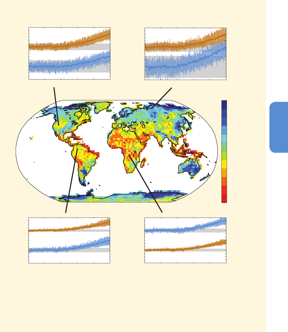
929

Detection and Attribution of Climate Change: from Global to Regional Chapter 10

FAQ 10.2, Figure 1 | Time series of projected temperature change shown at four representative locations for summer (red curves, representing June, July and August

at sites in the tropics and Northern Hemisphere or December, January and February in the Southern Hemisphere) and winter (blue curves). Each time series is surrounded

by an envelope of projected changes (pink for the local warm season, blue for the local cold season) yielded by 24 different model simulations, emerging from a grey

envelope of natural local variability simulated by the models using early 20th century conditions. The warming signal emerges ﬁrst in the tropics during summer. The

central map shows the global temperature increase (°C) needed for temperatures in summer at individual locations to emerge from the envelope of early 20th century

variability. Note that warm colours denote the smallest needed temperature increase, hence earliest time of emergence. All calculations are based on Coupled Model

Intercomparison Project Phase 5 (CMIP5) global climate model simulations forced by the Representative Concentration Pathway 8.5 (RCP8.5) emissions scenario.

Envelopes of projected change and natural variability are deﬁned as ±2 standard deviations. (Adapted and updated from Mahlstein et al., 2011.)

0.2

0.3

0.4

0.5

0.6

0.7

0.8

0.9

1.1

1.2

1.3

1.4

1900 1940 1980 2020 2060 2100

-8

-4

Year

DJF temperature anomaly (°C)

-8

-4

JJA temperature anomaly (°C)

1900 1940 1980 2020 2060 2100

-8

-4

Year

DJF temperature anomaly (°C)

-8

-4

JJA temperature anomaly (°C)

1900 1940 1980 2020 2060 2100

-8

-4

Year

DJF temperature anomaly (°C)

-8

-4

JJA temperature anomaly (°C)

1900 1940 1980 2020 2060 2100

-8

-4

Year

DJF temperature anomaly (°C)

-8

-4

JJA temperature anomaly (°C)

Global temperature increase (°C) needed for temperatures

in summer at individual locations to emerge from the

envelope of early 20th century variability

FAQ 10.2 (continued)

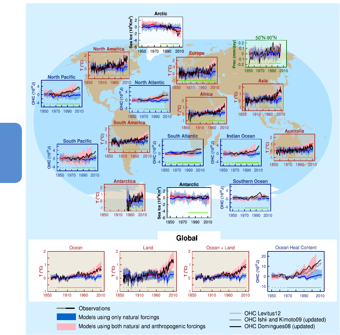
930

Chapter 10 Detection and Attribution of Climate Change: from Global to Regional

Figure 10.21 | Detection and attribution signals in some elements of the climate system, at regional scales (top panels) and global scales (bottom four panels). Brown panels are

land surface temperature time series, green panels are precipitation time series, blue panels are ocean heat content time series and white panels are sea ice time series. Observa-

tions are shown on each panel in black or black and shades of grey. Blue shading is the model time series for natural forcing simulations and pink shading is the combined natural

and anthropogenic forcings. The dark blue and dark red lines are the ensemble means from the model simulations. All panels show the 5 to 95% intervals of the natural forcing

simulations, and the natural and anthropogenic forcing simulations. For surface temperature the results are from Jones et al. (2013 ) (and Figure 10.1). The observed surface tem-

perature is from Hadley Centre/Climatic Research Unit gridded surface temperature data set 4 (HadCRUT4). Observed precipitation is from Zhang et al. (2007) (black line) and CRU

TS 3.0 updated (grey line). Three observed records of ocean heat content (OHC) are shown. Sea ice anomalies (rather than absolute values) are plotted and based on models in

Figure 10.16. The green horizontal lines indicate quality of the observations and estimates.For land and ocean surface temperatures panels and precipitation panels, solid green

lines at bottom of panels indicate where data spatial coverage being examined is above 50% coverage and dashed green lines where coverage is below 50%. For example, data

coverage of Antarctica never goes above 50% of the land area of the continent. For ocean heat content and sea ice panels the solid green line is where the coverage of data is

good and higher in quality, and the dashed green line is where the data coverage is only adequate. More details of the sources of model simulations and observations are given in

the Supplementary Material (10.SM.1).

931

Detection and Attribution of Climate Change: from Global to Regional Chapter 10

canic eruptions) cause much of the observed response (see also Figures

10.5, 10.6, 10.9, 10.14a and 10.21). Both natural and anthropogenic

forcings are required to understand fully the variability of the Earth

system during the past 50 years.

Water in the free atmosphere is expected to increase, as a consequence

of warming of the atmosphere (Section 10.6.1), and atmospheric circu-

lation controls the global distribution of precipitation and evaporation.

Simulations show that GHGs increase moisture in the atmosphere and

change its transport in such a way as to produce patterns of precipi-

tation and evaporation that are quite distinct from the observed pat-

terns of warming. Our assessment shows that anthropogenic forcings

have contributed to observed increases in moisture content in the

atmosphere (result 16, medium conﬁdence, Table 10.1), to global scale

changes in precipitation patterns over land (result 14, medium conﬁ-

dence), to a global scale intensiﬁcation of heavy precipitation in land

regions where there observational coverage is sufﬁcient to make an

assessment (result 15, medium conﬁdence), and to changes in surface

and sub-surface ocean salinity (result 11, very likely). Combining evi-

dence from both atmosphere and ocean that systematic changes in

precipitation over land and ocean salinity can be attributed to human

inﬂuence supports an assessment that it is likely that human inﬂuence

has affected the global water cycle since 1960.

Warming of the atmosphere and the oceans affects the cryosphere, and

in the case of snow and sea ice warming leads to positive feedbacks

that amplify the warming response in the atmosphere and oceans.

Retreat of mountain glaciers has been observed with an anthropo-

genic inﬂuence detected (result 17, likely, Table 10.1), Greenland ice

sheet has melted at the edges and accumulating snow at the higher

elevations is consistent with GHG warming supporting an assessment

for an anthropogenic inﬂuence on the negative surface mass balance

of Greenland’s ice sheet (result 18, likely, Table 10.1). Our level of sci-

entiﬁc understanding is too low to provide a quantiﬁable explanation

of the observed mass loss of the Antarctic ice sheet (low conﬁdence,

result 19, Table 10.1). Sea ice in the Arctic is decreasing rapidly and the

changes now exceed internal variability and with an anthropogenic

contribution detected (result 20, very likely, Table 10.1). Antarctic sea

ice extent has grown overall over the last 30 years but there is low sci-

entiﬁc understanding of the spatial variability and changes in Antarctic

sea ice extent (result 21, Table 10.1). There is evidence for an anthro-

pogenic component to observed reductions in NH snow cover since the

1970s (likely, result 22, Table 10.1).

Anthropogenic forcing has also affected temperature on continental

scales, with human inﬂuences having made a substantial contribution

to warming in each of the inhabited continents (results 28, likely, Table

10.1), and having contributed to the very substantial Arctic warming

over the past 50 years (result 29, likely, Table 10.1) while because of

large observational uncertainties there is low conﬁdence in attribution

of warming averaged over available stations over Antarctica (result 30,

Table 10.1). There is also evidence that anthropogenic forcings have

contributed to temperature change in many sub-continental regions

(result 32, likely, Table 10.1) and that anthropogenic forcings have

contributed to the observed changes in the frequency and intensity

of daily temperature extremes on the global scale since the mid-20th

century (result 8, very likely, Table 10.1). Furthermore there is evidence

that human inﬂuence has substantially increased the probability of

occurrence of heat waves in some locations (result 33, likely, Table

10.1).

An analysis of these results (from Table 10.1) shows that there is high

conﬁdence in attributing many aspects of changes in the climate

system to human inﬂuence including from atmospheric measurements

of temperature. Synthesizing the results in Table 10.1 shows that the

combined evidence from across the climate system increases the level

of conﬁdence in the attribution of observed climate change to human

inﬂuence and reduces the uncertainties associated with assessments

based on a single variable. From this combined evidence, it is virtually

certain that human inﬂuence has warmed the global climate system.

Acknowledgements

We acknowledge the major contributions of the following scientists

who took a substantial part in the production of key ﬁgures: Beena

Balan Sarojini, Oliver Browne, Jara Imbers Quintana, Gareth Jones,

Fraser Lott, Irina Mahlstein, Alexander Otto, Debbie Polson, Andrew

Schurer, Lijun Tao, and Muyin Wang. We also acknowledge the contri-

butions of Viviane Vasconcellos de Menezes for her work on the pro-

duction of ﬁgures and for her meticulous management of the bibliog-

raphy database used for this chapter.

932

Chapter 10 Detection and Attribution of Climate Change: from Global to Regional

Table 10.1 | Synthesis of detection and attribution results across the climate system from this chapter. Note that we follow the guidance note for lead authors of the IPCC AR5 on consistent treatment of uncertainties (Mastrandrea et al.,

2011). Where the conﬁdence is medium or less there is no assessment given of the quantiﬁed likelihood measure, and the table cell is marked not applicable (N/A).

Result (1) Statement about

variable or property:

time, season

(2) Conﬁdence

(Very high, High,

medium or low,

very low)

(3) Quantiﬁed measure of uncer-

tainty where the probability of

the outcome can be quantiﬁed

(Likelihood given generally only

if high or very high conﬁdence)

(4) Data sources

Observational evidence (Chapters 2

to 5); Models (Chapter 9)

(5) Type, amount, quality, consistency

of evidence from attribution studies

and degree of agreement of studies.

(6) Factors contributing to the assessments

including physical understanding, observational

and modelling uncertainty, and caveats.

Global Scale Atmospheric Temperature Changes

1 More than half of the

observed increase in global

mean surface temperatures

from 1951 to 2010 is due to

the observed anthropogenic

increase in greenhouse gas

(GHG) concentrations.

High Very likely Four global surface temperature series

(HadCRUT3, HadCRUT4, MLOST, GISTEMP).

CMIP3 and CMIP5 models.

· Many formal attribution studies,

including optimal ﬁngerprint time-space

studies and time series based studies.

· Robust evidence. Attribution of more

than half of warming since 1950 to

GHGs seen in multiple independent

analyses using different observational

data sets and climate models.

· High agreement. Studies agree in

robust detection of GHG contribu-

tion to observed warming that

is larger than any other factor

including internal variability.

The observed warming is well understood in terms

of contributions of anthropogenic forcings such

as greenhouse gases (GHGs) and tropospheric

aerosols and natural forcings from volcanic erup-

tions. Solar forcing is the only other forcing that

could explain long-term warming but pattern of

warming is not consistent with observed pattern

of change in time, vertical change and estimated

to be small. AMO could be confounding inﬂu-

ence but studies that ﬁnd signiﬁcant role for AMO

show this does not project strongly onto 60-year

trends. (Section 10.3.1.1, Figures 10.4 and 10.5)

2 More than half of the

observed increase in global

mean surface temperatures

from 1951 to 2010 is due to

human inﬂuence on climate.

High Extremely likely Mutliple CMIP5 models and

multiple methodologies.

· Formal attribution studies including

different optimal detection methodolo-

gies and time series based studies.

· Robust evidence of well-constrained

estimates of net anthropogenic warming

estimated in optimal detection studies.

· High agreement. Both optimal detec-

tion and time series studies agree in

robust detection of anthropogenic

inﬂuence that is substantially more

than half of the observed warming.

The observed warming is well understood in

terms of contributions of anthropogenic and

natural forcings. Solar forcing and AMO could be

confounding inﬂuence but are estimated to be

smaller than the net effects of human inﬂuence.

(Section 10.3.1.1, Figures 10.4, 10.5, 10.6)

3 Early 20th century warming is

due in part to external forcing.

High Very likely Instrumental global surface temperature

series and reconstructions of the last

millenium. CMIP3 and CMIP5 models.

· Formal detection and attribution studies

looking at early century warming and

studies for the last few hundred years.

· High agreement across a number

of studies in detecting external

forcings when including early 20th

century period although they vary in

contributions from different forcings.

Modelling studies show contribution from external

forcings to early century warming. Residual differ-

ences between models and observations indicate role

for circulation changes as contributor.

(Section 10.3.1.1, Figures 10.1, 10.2, 10.6)

4 Warming since 1950 cannot

be explained without external

forcing.

High Virtually certain Estimates of internal variability from CMIP3

and CMIP5 models, observation based

time series and space pattern analyses,

and estimating residuals of the non-forced

component from paleo data.

· Many, including optimal ﬁngerprint

time-space studies, observation

based time series and space pattern

analyses and paleo data studies.

· Robust evidence and high agreement.

· Detection of anthropogenic ﬁnger-

print robustly seen in independent

analyses using different observa-

tional data sets, climate models,

and methodological approaches.

Based on all evidence above combined. Observed

warming since 1950 is very large compared to climate

model estimates of internal variability, which are

assessed to be adequate at global scale. The Northern

Hemisphere (NH) mean warming since 1950 is far out-

side the range of any similar length trend in residuals

from reconstructions of NH mean temperature of

the past millennium. The spatial pattern of observed

warming differs from those associated with internal

variability. (Sections 9.5.3.1, 10.3.1.1, 10.7.1)

(continued on next page)

933

Detection and Attribution of Climate Change: from Global to Regional Chapter 10

Result

(1) Statement about

variable or property:

time, season

(2) Conﬁdence

(Very high, High,

medium or low,

very low)

(3) Quantiﬁed measure of uncer-

tainty where the probability of

the outcome can be quantiﬁed

(Likelihood given generally only

if high or very high conﬁdence)

(4) Data sources

Observational evidence (Chapters 2

to 5); Models (Chapter 9)

(5) Type, amount, quality, consistency

of evidence from attribution studies

and degree of agreement of studies.

(6) Factors contributing to the assessments

including physical understanding, observational

and modelling uncertainty, and caveats.

5 Anthropogenic forcing

has led to a detectable

warming of troposphere

temperatures since 1961.

High Likely Multiple radiosonde data sets from

1958 and satellite data sets from 1979

to present. CMIP3 and CMIP5 models.

· Formal attribution studies with CMIP3

models (assessed in AR4) and CMIP5

models.

· Robust detection and attribution of

anthropogenic inﬂuence on

tropospheric warming with large

signal-to-noise (S/N) ratios estimated.

· Studies agree in detecting an anthropo-

genic inﬂuence on tropospheric

warming trends.

Observational uncertainties in radiosondes are

now much better documented than at time of

AR4. It is virtually certain that the troposphere has

warmed since the mid-20th century but there is

only medium conﬁdence in the rate and vertical

structure of those changes in the NH extratropi-

cal troposphere and low conﬁdence elsewhere.

Most, though not all, CMIP3 and CMIP5 models

overestimate the observed warming trend in the

tropical troposphere during the satellite period

although observational uncertainties are large

and outside the tropics and over the period of the

radiosonde record beginning in 1961 there is better

agreement between simulated and observed trends.

(Sections 2.4.4, 9.4.1.4.2, 10.3.1.2, Figure 10.8)

6 Anthropogenic forcing

dominated by the depletion

of the ozone layer due to

ozone depleting substances,

has led to a detectable

cooling of lower stratosphere

temperatures since 1979.

High Very Likely Radiosonde data from 1958 and satellite

data from 1979 to present. CCMVal,

CMIP3 and CMIP5 simulations.

· A formal optimal detection attribution

study using stratosphere resolving

chemistry climate models and a

detection study analysing the S/N

ratio of the data record together

with many separate modelling

studies and observational studies.

· Physical reasoning and model studies

show very consistent understanding

of observed evolution of stratospheric

temperatures, consistent with formal

detection and attribution results.

· Studies agree in showing very strong

cooling in stratosphere that can be

explained only by anthropogenic

forcings dominated by ozone

depleting substances.

New generation of stratosphere resolving models

appear to have adequate representation of lower

stratospheric variability. Structure of stratospheric

temperature trends and variations is reasonably

well represented by models. CMIP5 models all

include changes in stratospheric ozone while only

about half of the models participating in CMIP3

include stratospheric ozone changes. (Sections

9.4.1.4.5, 10.3.1.2.2, Figures10.8 and 10.9)

7 Anthropogenic forcing, particu-

larly GHGs and stratospheric

ozone depletion has led to a

detectable observed pattern

of tropospheric warming

and lower stratospheric

cooling since 1961.

High Very likely Radiosonde data from 1958 and

satellite data from 1979 to present.

· Attribution studies using CMIP3 and

CMIP5 models.

· Physical reasoning and modelling sup-

ports robust expectation of ﬁngerprint

of anthropogenic inﬂuence of tropo-

spheric warming and lower stratospheric

cooling which is robustly detected

in multiple observational records.

· Fingerprint of anthropogenic inﬂuence

is detected in different measures of

free atmosphere temperature changes

including tropospheric warming,

and a very clear identiﬁcation of

stratospheric cooling in models that

include anthropogenic forcings.

Fingerprint of changes expected from physical under-

standing and as simulated by models is detected in

observations. Understanding of stratospheric changes

has improved since AR4. Understanding of obser-

vational uncertainty has improved although uncer-

tainties remain particularly in the tropical upper tropo-

sphere. (Sections 2.4.4, 10.3.1.2.3, Figures 10.8, 10.9)

(continued on next page)

Table 10.1 (continued)

934

Chapter 10 Detection and Attribution of Climate Change: from Global to Regional

Result

(1) Statement about

variable or property:

time, season

(2) Conﬁdence

(Very high, High,

medium or low,

very low)

(3) Quantiﬁed measure of uncer-

tainty where the probability of

the outcome can be quantiﬁed

(Likelihood given generally only

if high or very high conﬁdence)

(4) Data sources

Observational evidence (Chapters 2

to 5); Models (Chapter 9)

(5) Type, amount, quality, consistency

of evidence from attribution studies

and degree of agreement of studies.

(6) Factors contributing to the assessments

including physical understanding, observational

and modelling uncertainty, and caveats.

8 Anthropogenic forcing has

contributed to the observed

changes in the frequency and

intensity of daily temperatures

extremes on the global scale

since the mid-20th century.

High Very Likely Indices for frequency and intensity of

extreme temperatures including annual

maximum and annual minimum daily

temperatures, over land areas of the

World except parts of Africa, South

America and Antarctica. CMIP3 and

CMIP5 simulations, 1950–2005.

· Several studies including ﬁngerprint

time–space studies.

· Detection of anthropogenic inﬂuence

robustly seen in independent analysis

using different statistical methods and

different indices.

Expected from physical principles that changes in

mean temperature should bring changes in extremes,

conﬁrmed by detection and attribution studies.

New evidence since AR4 for detection of human

inﬂuence on extremely warm daytime maximum

temperatures and new evidence that inﬂuence of

anthropogenic forcing can be separately detected

from natural forcing. More limited observational

data and greater observational uncertainties than for

mean temperatures. (Section 10.6.1.1, Figure 10.17)

Oceans

9 Anthropogenic forcings

have made a substantial

contribution to upper ocean

warming (above 700 m)

observed since the 1970s.

This anthropogenic ocean

warming has contrib-

uted to global sea level rise

over this period through

thermal expansion.

High Very likely Several observational data sets since

the 1970s. CMIP3 and CMIP5 models.

· Several new attribution studies detect

role of anthropogenic forcing on

observed increase in ocean’s global

heat content with volcanic forcing also

contributing to observed variability.

· The evidence is very robust, and tested

against known structural deﬁciencies

in the observations, and in the models.

· High levels of agreement across attribu-

tion studies and observation and model

comparison studies. The strong physical

relationship between thermosteric sea

level and ocean heat content means that

the anthropogenic ocean warming has

contributed to global sea level rise over

this period through thermal expansion.

New understanding of the structural errors in the

temperature data sets has led to their correction

which means that the unexplained multi-decadal

scale variability reported in AR4 has largely been

resolved as being spurious. The observations and

climate simulations have similar trends (including

anthropogenic and volcanic forcings) and similar

decadal variability. The detection is well above S/N

levels required at 1 and 5% signiﬁcance levels.

The new results show the conclusions to be very

robust to structural uncertainties in observational

data sets and transient climate simulations. (Sec-

tions 3.2.5, 10.4.1, 10.4.3, 13.3.6, Figure 10.14)

10 Anthropogenic forcing has

contributed to sea level rise

through melting glaciers

and Greenland ice sheet.

High Likely Observational evidence of melting glaciers

(Section 4.3) and ice sheets (Section 4.4).

Global mean sea level budget closure to

within uncertainties. (Section13.3.6)

· Several new mass balance studies

quantifying glacier and ice sheet melt

rates (Section 10.5.2) and their contribu-

tions to sea level rise. (Section 13.3)

Strong observational evidence of contribution from

melting glaciers and high conﬁdence in attribution of

glacier melt to human inﬂuence. Increasing rates of

ice sheet contributions albeit from short observa-

tional record (especially of Antarctic mass loss).

Current climate models do not represent

glacier and ice sheet processes. Natural vari-

ability of glaciers and ice sheets not fully

understood. (Sections 10.4.3, 10.5.2)

(continued on next page)

Table 10.1 (continued)

935

Detection and Attribution of Climate Change: from Global to Regional Chapter 10

Result

(1) Statement about

variable or property:

time, season

(2) Conﬁdence

(Very high, High,

medium or low,

very low)

(3) Quantiﬁed measure of uncer-

tainty where the probability of

the outcome can be quantiﬁed

(Likelihood given generally only

if high or very high conﬁdence)

(4) Data sources

Observational evidence (Chapters 2

to 5); Models (Chapter 9)

(5) Type, amount, quality, consistency

of evidence from attribution studies

and degree of agreement of studies.

(6) Factors contributing to the assessments

including physical understanding, observational

and modelling uncertainty, and caveats.

11 The observed ocean surface

and sub-surface salinity chang-

es since the 1960s are due, in

part, to anthropogenic forcing.

High Very likely Oceans chapter (Section 3.3) and

attribution studies in Section 10.4.2.

· Robust observational evidence for

ampliﬁcation of climatological patterns

of surface salinity.

· CMIP3 simulations show patterns of

salinity change consistent with observa-

tions, but there are only a few formal

attributions studies that include a full

characterization of internal variability.

· Physical understanding of expected

patterns of change in salinity due to

changes in water cycle support results

from detection and attriution studies.

More than 40 studies of regional, global surface and

subsurface salinity observations show patterns of

change consistent with acceleration of hydrological

water cycle. Climate models that include anthropgenic

forcings show the same consistent pattern of surface

salinity change. (Sections 3.3.5, 10.4.2, Figure 10.15)

12 Observed increase in

surface ocean acidiﬁcation

since 1980s is a resulted of

rising atmospheric CO

Very high Very likely Evidence from Section 3.8.2

and Box 3.2, Figure 3.18.

· Based on ocean chemistry, expert

judgement, and many analyses of time

series and other indirect measurements

· Robust evidence from time series

measurements. Measurements

have a high degree of certainty (see

Table 3.2) and instrumental records

show increase in ocean acidity.

· High agreement of the observed trends.

Very high conﬁdence, based on the number of studies,

the updates to earlier results in AR4, and the very well

established physical understanding of gas exchange

between atmosphere and surface ocean, and the

sources of excess carbon dioxide in the atmosphere.

Alternative processes and hypotheses can be

excluded. (Section 3.8.2, Box 3.2, Section 10.4.4)

13 Observed pattern of

decrease in oxygen content

is, in part, attributable to

anthropogenic forcing.”

To correctly read: Observed

pattern of decrease in oxygen

content from the 1960s to the

1990s is, in part, attributable

to anthropogenic forcing.

Medium About as likely as not Evidence from Section 3.8.3 and

attribution studies in Section 10.4.4.

· Qualitative expert judgement based on

comparison of observed and expected

changes in response to increasing CO

· Medium evidence. One speciﬁc global

ocean study, many studies of hydro-

graphic sections and repeat station

data, high agreement across

observational studies.

· Medium agreement. One attri-

bution study, and only limited

regional and large-scale modelling

and observation comparisons.

Physical understanding of ocean circulation and

ventilation, and from the global carbon cycle, and

from simulations of ocean oxygen concentrations

from coupled bio-geochemical models with OAGCMs.

Main uncertainty is observed decadal variability which

is not well understood in global and regional

inventories of dissolved oxygen in the oceans.

(Section 10.4.4)

Water Cycle

14 Global scale precipitation

patterns over land have

changed due to anthropogenic

forcings including increases

in NH mid to high latitudes.

Medium N/A Multiple observational data sets

based on rain gauges over land,

with coverage dominated by the

NH. CMIP3 and CMIP5 models.

· Several land precipitation studies exam-

ining annual and seasonal precipitation.

· Evidence for consistency between

observed and modelled changes in

global precipitation patterns over land

regions with sufﬁcient observations.

· Medium degree of agreement of studies.

Expected anthropogenic ﬁngerprints

of changes in zonal mean precipitation

found in annual and some seasonal

data with some sensitivity of attribution

results to observational data set used.

Increases of precipitation at high latitudes of the NH

are a robust feature of climate model simulations

and are expected from process understanding.

Global-land average long-term changes small at

present time, whereas decadal variability over some

land areas is large. Observations are very uncertain

and poor coverage of precipitation expected to

make ﬁngerprint of changes much more indistinct.

(Sections 2.5.1, 10.3.2.2, Figures 10.10 and 10.11)

(continued on next page)

Table 10.1 (continued)

936

Chapter 10 Detection and Attribution of Climate Change: from Global to Regional

Result

(1) Statement about

variable or property:

time, season

(2) Conﬁdence

(Very high, High,

medium or low,

very low)

(3) Quantiﬁed measure of uncer-

tainty where the probability of

the outcome can be quantiﬁed

(Likelihood given generally only

if high or very high conﬁdence)

(4) Data sources

Observational evidence (Chapters 2

to 5); Models (Chapter 9)

(5) Type, amount, quality, consistency

of evidence from attribution studies

and degree of agreement of studies.

(6) Factors contributing to the assessments

including physical understanding, observational

and modelling uncertainty, and caveats.

15 In land regions where

observational coverage is

sufﬁcient for assessment,

anthropogenic forcing has

contributed to global-scale

intensiﬁcation of heavy

precipitation over the second

half of the 20th century.

Medium N/A Wettest 1-day and 5-day precipitation

in a year obtained from rain guage

observations, CMIP3 simulations.

· Only one detection and attribution

study restricted to NH land where

observations were available.

· Study found stronger detectability

for models with natural forcings but

not able to differentiate anthro-

pogenic from natural forcings.

· Although only one formal detection

and attribution study, observa-

tions of a general increase in heavy

precipitation at the global scale

agree with physical expectations.

Evidence for anthropogenic inﬂuence on vari-

ous aspects of the hydrological cycle that implies

extreme precipitation would be expected to

increase. There are large observational uncertainties

and poor global coverage which makes assess-

ment difﬁcult. (Section 10.6.1.2, Figure 10.11)

16 Anthropogenic contribu-

tion to atmospheric speciﬁc

humidity since 1973.

Medium N/A Observations of atmospheric moisture

content over ocean from satellite; observa-

tions of surface humidity from weather

stations and radiosondes over land.

· Detection and attribution studies of

both surface humidity from weather sta-

tions over land and atmospheric mois-

ture content over oceans from satellites.

· Detection of anthropogenic inﬂuence

on atmospheric moisture content over

oceans robust to choice of models.

· Studies looking at different variables

agree in detecting speciﬁc humidity

changes.

Recent reductions in relative humidity over land and

levelling off of speciﬁc humidity not fully under-

stood. Length and quality of observational data

sets limit detection and attribution and assimi-

lated analyses not judged sufﬁciently reliable for

detection and attribution. (Section 10.3.2.1)

Hemispheric Scale Changes; Basin Scale Changes

Cryosphere

17 A substantial part of glaciers

mass loss since the 1960’s

is due to human inﬂuence.

High Likely Robust agreement from

long-term glacier records. (Section 4.3.3)

· Several new recent studies since last

assessment.

· High agreement across a limited

number of studies.

Well established records of glacier length, and better

methods of estimating glacier volumes and

mass loss. Better characterization of internal variability,

and better understanding of the response to natural

variability, and local land cover change. (Sections

4.3.3, 10.5.2)

18 Anthropogenic forcing

has contributed to surface

melting of the Greenland

ice sheet since 1993.

High Likely Robust agreement across in situ and

satellite derived estimates of surface

mass balance (Section 4.4). Nested or

downscaled model simulations show pat-

tern of change consistent with warming.

· Several new studies since last

assessment.

· Robust evidence from different sources.

· High agreement across a limited number

of studies.

Documented evidence of surface mass loss. Uncer-

tainty caused by poor characterization of the internal

variability of the surface mass balance (strong depen-

dence on atmospheric variability) that is not well

represented in CMIP5 models. (Section 4.4.2, 10.5.2.1)

19 Antarctic ice sheet mass bal-

ance loss has a contribution

from anthropogenic forcing.

Low N/A Observational evidence for Antarctic mass

sheet loss is well established across a

broad range of studies. (Section 4.4)

· No formal studies exist. Processes for

mass loss for Antarctica are not well

understood. Regional warming and

changed wind patterns (increased

westerlies, increase in the Southern

Annular Mode (SAM)) could contribute

to enhanced melt of Antarctica. High

agreement in observational studies.

Low conﬁdence assessment based on low scientiﬁc

understanding. (Sections 4.4.2, 13.4, 10.5.2)

20 Anthropogenic forcing has

contributed to the Arctic

sea ice loss since 1979.

High Very likely Robust agreement across all

observations. (Section 4.2)

· Multiple detection and attribution

studies, large number of model simula-

tions and data comparisons for

instrumental record.

· Robust set of studies of simulations of

sea ice and observed sea ice extent.

· High agreement between stud-

ies of sea ice simulations and

observed sea ice extent.

High conﬁdence based on documented observa-

tions of ice extent loss, and also good evidence

for a signiﬁcant reduction in sea ice volume. The

physics of Arctic sea ice is well understood and

consistent with the observed warming in the region,

and from simulations of Arctic sea ice extent with

anthropogenic forcing. (Sections 9.4.3, 10.5.1)

(continued on next page)

Table 10.1 (continued)

937

Detection and Attribution of Climate Change: from Global to Regional Chapter 10

Result

(1) Statement about

variable or property:

time, season

(2) Conﬁdence

(Very high, High,

medium or low,

very low)

(3) Quantiﬁed measure of uncer-

tainty where the probability of

the outcome can be quantiﬁed

(Likelihood given generally only

if high or very high conﬁdence)

(4) Data sources

Observational evidence (Chapters 2

to 5); Models (Chapter 9)

(5) Type, amount, quality, consistency

of evidence from attribution studies

and degree of agreement of studies.

(6) Factors contributing to the assessments

including physical understanding, observational

and modelling uncertainty, and caveats.

21 Incomplete scientiﬁc explana-

tions of the observed increase

in Antarctic sea ice extent pre-

cludes attribution at this time.

N/A N/A The increase in sea ice extent in

observations is robust, based on

satellite measurements and ship-based

measurements. (Section 4.5.2)

· No formal attribution studies.

· Estimates of internal variability from

CMIP5 simulations exceed observed

sea ice variability.

· Modelling studies have a low level of

agreement for observed increase, and

there are competing scientiﬁc

explanations.

Low conﬁdence based on low scientiﬁc understand-

ing of the spatial variability and changes in the

Antarctic sea ice. (Sections 4.5.2, 10.5.1, 9.4.3)

22 There is an anthropogenic com-

ponent to observed reductions

in NH snow cover since 1970

High Likely Observations show decrease

in NH snow cover.

· Two snow cover attribution studies.

· Decrease in snow cover in the

observations are consistent among

many studies. (Section 4.5.2, 4.5.3)

· Reductions in observed snow cover

inconsistent with internal variability and

can be explained only by climate models

that include anthropogenic forcings.

Expert judgement and attribution studies sup-

port the human inﬂuence on reduction in snow

cover extent. (Sections 4.5.2, 4.5.3, 10.5.3)

Atmospheric Circulation and Patterns of Variability

23 Human inﬂuence has altered

sea level pressure patterns

globally since 1951.

High Likely An observational gridded data set and

reanalyses. Multiple climate models.

· A number of studies ﬁnd detectable

anthropogenic inﬂuence on sea level

pressure patterns.

· Detection of anthropogenic inﬂuence is

found to be robust to currently sampled

modelling and observational uncertainty.

Detectable anthropogenic inﬂuence on changes

in sea level pressure patterns is found in several

attribution studies that sample observational and

modelling uncertainty. Observational uncertainties

not fully sampled as results based largely on variants

of one gridded data set although analyses based on

reanalyses also support the ﬁnding of a detectable

anthropogenic inﬂuence. (Section 10.3.3.4)

24 The positive trend in the

SAM seen in austral summer

since 1951 is due in part to

stratospheric ozone depletion.

High Likely Measurements since 1957. Clear

signal of SAM trend in December,

January and February (DJF) is robust

to observational uncertainty.

· Many studies comparing consistency

of observed and modelled trends, and

consistency of observed trend with

simulated internal variability.

· Observed trends are consistent with

CMIP3 and CMIP5 simulations that

include stratospheric ozone depletion.

· Several studies show that the

observed increase in the DJF SAM is

inconsistent with simulated internal

variability. High agreement of model-

ling studies that ozone depletion

drives an increase in the DJF SAM

index. There is medium conﬁdence

that GHGs have also played a role.

Consistent result of modelling studies is that

the main aspect of the anthropogenically forced

response on the DJF SAM is the impact of ozone

depletion. The observational record is relatively

short, observational uncertainties remain, and

the DJF SAM trend since 1951 is only margin-

ally inconsistent with internal variability in some

data sets. (Section 10.3.3.3, Figure 10.13)

25 Stratospheric ozone deple-

tion has contributed to the

observed poleward shift of

the Southern Hadley cell

during austral summer.

Medium N/A Multiple observational lines of

evidence for widening but large

spread in the magnitude.

Reanalysis suggest a southward

shift of southern Hadley cell border

during DJF which is also seen in

CMIP3 and CMIP5 models.

· Consistent evidence for effects of

stratospheric ozone depletion.

· Evidence from modelling studies is

robust that stratospheric ozone drives

a poleward shift of the southern Hadley

Cell border during austral summer. The

magnitude of the shift is very uncertain

and appears to be underestimated by

models. There is medium conﬁdence

that GHGs have also played a role.

The observed magnitude of the tropical belt

widening is uncertain. The contribution of internal

climate variability to the observed poleward

expansion of the Hadley circulation remains very

uncertain. (Section 10.3.3.1, Figure 10.12)

(continued on next page)

Table 10.1 (continued)

938

Chapter 10 Detection and Attribution of Climate Change: from Global to Regional

Result

(1) Statement about

variable or property:

time, season

(2) Conﬁdence

(Very high, High,

medium or low,

very low)

(3) Quantiﬁed measure of uncer-

tainty where the probability of

the outcome can be quantiﬁed

(Likelihood given generally only

if high or very high conﬁdence)

(4) Data sources

Observational evidence (Chapters 2

to 5); Models (Chapter 9)

(5) Type, amount, quality, consistency

of evidence from attribution studies

and degree of agreement of studies.

(6) Factors contributing to the assessments

including physical understanding, observational

and modelling uncertainty, and caveats.

26 Attribution of changes in

tropical cyclone activity

to human inﬂuence.

Low N/A Incomplete and short observa-

tional records in most basins.

· Formal attribution studies on SSTs

in tropics. However, mechanisms

linking anthropogenically induced

SST increases to changes in tropical

cyclone activity poorly understood.

· Attribution assessments depend on

multi-step attribution linking anthro-

pogenic inﬂuence to large-scale drivers

and thence to tropical cyclone activity.

· Low agreement between studies,

medium evidence.

Insufﬁcient observational evidence of multi-decadal

scale variability. Physical understanding lacking.

There remains substantial disagreement on the

relative importance of internal variability, GHG

forcing, and aerosols. (Sections 10.6.1.5, 14.6.1)

Millennium Time Scale

27 External forcing contrib-

uted to NH temperature

variability from 1400 to 1850,

and from 850 to 1400.

High for period

from 1400 to 1850;

medium for period

from 850 to 1400.

Very likely for period

from 1400 to 1850.

See Chapter 5 for reconstructions;

simulations from PMIP3 and CMIP5

models, with more robust detec-

tion results for 1400 onwards.

· A small number of detection and

attribution studies and further evidence

from climate modelling studies; com-

parison of models with reconstructions

and results from data assimilation.

· Robust agreement from a number of

studies using a range of reconstruc-

tions and models (EBMs to ESMs)

that models are able to reproduce

key features of last seven centuries.

· Detection results and simulations

indicate a contribution by external

drivers to the warm conditions in

the 11th to 12th century, but cannot

explain the warmth around the 10th

century in some reconstructions.

Large uncertainty in reconstructions particularly for

the ﬁrst half of the millennium but good agreement

between reconstructed and simulated large scale fea-

tures from 1400. Detection of forced inﬂuence robust

for a large range of reconstructions. Difﬁcult to sepa-

rate role of individual forcings. Results prior to 1400

much more uncertain, partly due to larger data and

forcing uncertainty. (Sections 10.7.1, 10.7.2, 10.7.3)

Continental to Regional Scale Changes

28 Anthropogenic forcing has

made a substantial contribu-

tion to warming to each of

the inhabited continents.

High Likely Robust observational evidence except

for Africa due to poor sampling.

Detection and attribution studies

with CMIP3 and CMIP5 models.

· New studies since AR4 detect

anthropogenic warming on continental

and sub-continental scales.

· Robust detection of human inﬂuence on

continental scales agrees with global

attribution of widespread warming over

land to human inﬂuence.

· Studies agree in detecting human

inﬂuence on continental scales.

Anthropogenic pattern of warming widespread

across all inhabited continents. Lower S/N ratios at

continental scales than global scales. Separation of

response to forcings more difﬁcult at these scales.

Models have greater errors in representation of

regional details. (Section 10.3.1.1,4, Box 11.2)

29 Anthropogenic contribution to

very substantial Arctic warm-

ing over the past 50 years.

High Likely Adequate observational coverage since

1950s.

Detection and attribution analy-

sis with CMIP3 models.

· Multiple models show ampliﬁcation of

Arctic temperatures from anthropogenic

forcing.

· Large positive Arctic-wide temperature

anomalies in observations over last

decade and models are consistent only

when they include external forcing.

Large temperature signal relative to mid-latitudes but

also larger internal variability and poorer obser-

vational coverage than at lower latitudes. Known

multiple processes including albedo shifts and added

heat storage contribute to faster warming than at

lower latitudes. (Sections 10.3.1.1.4. 10.5.1.1)

(continued on next page)

Table 10.1 (continued)

939

Detection and Attribution of Climate Change: from Global to Regional Chapter 10

Result

(1) Statement about

variable or property:

time, season

(2) Conﬁdence

(Very high, High,

medium or low,

very low)

(3) Quantiﬁed measure of uncer-

tainty where the probability of

the outcome can be quantiﬁed

(Likelihood given generally only

if high or very high conﬁdence)

(4) Data sources

Observational evidence (Chapters 2

to 5); Models (Chapter 9)

(5) Type, amount, quality, consistency

of evidence from attribution studies

and degree of agreement of studies.

(6) Factors contributing to the assessments

including physical understanding, observational

and modelling uncertainty, and caveats.

30 Human contribution

to observed warming

averaged over available

stations over Antarctica.

Low N/A Poor observational coverage of Antarc-

tica with most observations around the

coast. Detection and attribution studies

with CMIP3 and CMIP5 models.

· One optimal detection study, and some

modelling studies.

· Clear detection in one optimal detection

study.

Possible contribution to changes from SAM increase.

Residual when SAM induced changes are removed

shows warming consistent with expectation due to

anthropogenic forcing. High observational uncertainty

and sparse data coverage (individual stations only

mostly around the coast). (Sections 10.3.1.1.4, 2.4.1.1)

31 Contribution by forcing to

reconstructed European

temperature variability over

last ﬁve centuries.

Medium N/A European seasonal tempera-

tures from 1500 onwards.

· One detection and attribution study and

several modelling studies.

· Clear detection of external forcings in

one study; robust volcanic signal seen

in several studies (see also Chapter 5).

Robust volcanic response detected in Epoch analyses

in several studies. Models reproduce low-frequency

evolution when include external forcings. Uncertainty

in overall level of variability, uncertainty in

reconstruction particularly prior to late 17th century.

(Sections 10.7.2, 5.5.1)

32 Anthropogenic forcing has

contributed to temperature

change in many sub-conti-

nental regions of the world.

High Likely Good observational coverage for

many regions (e.g., Europe) and

poor for others (e.g., Africa, Arctic).

Detection and attribution studies

with CMIP3 and CMIP5 models.

· A number of detection and attribution

studies have analysed temperatures

on scales from Giorgi regions to

climate model grid box scale.

· Many studies agree in showing that

an anthropogenic signal is appar-

ent in many sub-continental scale

regions. In some sub-continental-

scale regions circulation changes

may have played a bigger role.

Larger role of internal variability at smaller scales

relative to signal of climate change. In some regions

observational coverage is poor. Local forcings

and feedbacks as well as circulation changes are

important in many regions and may not be well

simulated in all regions. (Section 10.3.1.1.4, Box 11.2)

33 Human inﬂuence has

substantially increased the

probability of occurrence of

heat waves in some locations.

High Likely Good observational coverage for some

regions and poor for others (thus biasing

studies to regions where observational

coverage is good). Coupled modeling stud-

ies examining the effects of anthropogonic

warming and the probability of occurrence

of very warm seasonal temperatures and

targeted experiments with models forced

with prescribed sea surface temperatures.

· Multi-step attribution studies of some

events including the Europe 2003,

Western Russia 2010, and Texas 2011

heatwaves have shown an anthropo-

genic contribution to their occurrence

probability, backed up by studies

looking at the overall implications of

increasing mean temperatures for the

probability of exceeding seasonal mean

temperature thresholds in some regions.

· To infer the probability of a heatwave,

extrapolation has to be made from the

scales on which most attribution studies

have been carried out to the spatial

and temporal scales of heatwaves.

· Studies agree in ﬁnding robust evidence

for anthropogenic inﬂuence on increase

in probability of occurrence of extreme

seasonal mean temperatures in many

regions.

In some instances, circulation changes could be more

important than thermodynamic changes. This could

be a possible confounding inﬂuence since much of

the magnitude (as opposed to the probability of

occurrence) of many heat waves is attributable to

atmospheric ﬂow anomalies. (Sections 10.6.1, 10.6.2)

Table 10.1 (continued)

940

Chapter 10 Detection and Attribution of Climate Change: from Global to Regional

References

AchutaRao, K. M., B. D. Santer, P. J. Gleckler, K. E. Taylor, D. W. Pierce, T. P. Barnett, and

T. M. L. Wigley, 2006: Variability of ocean heat uptake: Reconciling observations

and models. J. Geophys. Res. Oceans, 111, C05019.

AchutaRao, K. M., et al., 2007: Simulated and observed variability in ocean

temperature and heat content. Proc. Natl. Acad. Sci. U.S.A., 104, 10768–10773.

Ahlmann, H. W., 1948: The present climatic ﬂuctuation. Geogr.J., 112, 165–195.

Aldrin, M., M. Holden, P. Guttorp, R. B. Skeie, G. Myhre, and T. K. Berntsen, 2012:

Bayesian estimation of climate sensitivity based on a simple climate model

ﬁtted to observations of hemispheric temperatures and global ocean heat

content. Environmetrics, 23, 253–271.

Alekseev, G. V., A. I. Danilov, V. M. Kattsov, S. I. Kuz’mina, and N. E. Ivanov, 2009:

Changes in the climate and sea ice of the Northern Hemisphere in the 20th and

21st centuries from data of observations and modeling. Izvestiya Atmospheric

and Oceanic Physics, 45, 675–686.

Alexander, L. V., and J. M. Arblaster, 2009: Assessing trends in observed and modelled

climate extremes over Australia in relation to future projections. Int. J. Climatol.,

29, 417–435.

Allan, R., and T. Ansell, 2006: A new globally complete monthly historical gridded

mean sea level pressure dataset (HadSLP2): 1850–2004. J. Clim., 19, 5816–5842.

Allan, R. P., B. J. Soden, V. O. John, W. Ingram, and P. Good, 2010: Current changes in

tropical precipitation. Environ. Res. Lett., 5, 025205.

Allen, M., 2011: In defense of the traditional null hypothesis: Remarks on the

Trenberth and Curry WIREs opinion articles. WIREs Clim. Change, 2, 931–934.

Allen, M. R., and S. F. B. Tett, 1999: Checking for model consistency in optimal

ﬁngerprinting. Clim. Dyn., 15, 419–434.

Allen, M. R., and W. J. Ingram, 2002: Constraints on future changes in climate and

the hydrologic cycle. Nature, 419, 224–232.

Allen, M. R., and P. A. Stott, 2003: Estimating signal amplitudes in optimal

ﬁngerprinting. Part I: Theory. Clim. Dyn., 21, 477–491.

Allen, M. R., P. A. Stott, J. F. B. Mitchell, R. Schnur, and T. L. Delworth, 2000: Quantifying

the uncertainty in forecasts of anthropogenic climate change. Nature, 407,

617–620.

Allen, M. R., D. J. Frame, C. Huntingford, C. D. Jones, J. A. Lowe, M. Meinshausen,

and N. Meinshausen, 2009: Warming caused by cumulative carbon emissions

towards the trillionth tonne. Nature, 458, 1163–1166.

Allen, M. R., et al., 2006: Quantifying anthropogenic inﬂuence on recent near-surface

temperature change. Surv. Geophys., 27, 491–544.

Allen, R. J., S. C. Sherwood, J. R. Norris, and C. S. Zender, 2012: Recent Northern

Hemisphere tropical expansion primarily driven by black carbon and tropospheric

ozone. Nature, 485, 350–354.

Ammann, C. M., and E. R. Wahl, 2007: The importance of the geophysical context in

statistical evaluations of climate reconstruction procedures. Clim. Change, 85,

71–88.

Ammann, C. M., F. Joos, D. S. Schimel, B. L. Otto-Bliesner, and R. A. Tomas, 2007:

Solar inﬂuence on climate during the past millennium: Results from transient

simulations with the NCAR Climate System Model. Proc. Natl. Acad. Sci. U.S.A.,

104, 3713–3718.

Andreae, M. O., C. D. Jones, and P. M. Cox, 2005: Strong present-day aerosol cooling

implies a hot future. Nature, 435, 1187–1190.

Andrews, O. D., N. L. Bindoff, P. R. Halloran, T. Ilyina, and C. Le Quéré, 2013: Detecting

an external inﬂuence on recent changes in oceanic oxygen using an optimal

ﬁngerprinting method. Biogeosciences, 10, 1799–1813.

Annan, J. D., and J. C. Hargreaves, 2006: Using multiple observationally-based

constraints to estimate climate sensitivity. Geophys. Res. Lett., 33, L06704.

Annan, J. D., and J. C. Hargreaves, 2010: Reliability of the CMIP3 ensemble. Geophys.

Res. Lett., 37, L02703.

Annan, J. D., and J. C. Hargreaves, 2011: On the generation and interpretation of

probabilistic estimates of climate sensitivity. Clim. Change, 104, 423–436.

Aoki, S., N. L. Bindoff, and J. A. Church, 2005: Interdecadal water mass changes in

the Southern Ocean between 30 degrees E and 160 degrees E. Geophys. Res.

Lett., 32, L07607.

Arkin, P. A., T. M. Smith, M. R. P. Sapiano, and J. Janowiak, 2010: The observed

sensitivity of the global hydrological cycle to changes in surface temperature.

Environ. Res. Lett., 5, 035201.

Bal, S., S. Schimanke, T. Spangehl, and U. Cubasch, 2011: On the robustness of the

solar cycle signal in the Paciﬁc region. Geophys. Res. Lett., 38, L14809.

Balachandran, N. K., D. Rind, P. Lonergan, and D. T. Shindell, 1999: Effects of solar

cycle variability on the lower stratosphere and the troposphere. J. Geophys. Res.

Atmos., 104, 27321–27339.

Balan Sarojini, B., P. Stott, E. Black, and D. Polson, 2012 Fingerprints of changes in

annual and seasonal precipitation from CMIP5 models over land and ocean.

Geophys. Res. Lett., 39, L23706.

Barnett, T. P., D. W. Pierce, and R. Schnur, 2001: Detection of anthropogenic climate

change in the world’s oceans. Science, 292, 270–274.

Barnett, T. P., D. W. Pierce, K. Achutarao, P. Gleckler, B. Santer, J. Gregory, and W.

Washington, 2005: Penetration of human-induced warming into the world’s

oceans. Science, 309, 284–287.

Barnett, T. P., et al., 2008: Human-induced changes in the hydrology of the western

United States. Science, 319, 1080–1083.

Barriopedro, D., R. Garcia-Herrera, and R. Huth, 2008: Solar modulation of Northern

Hemisphere blocking. J. Geophys. Res. Atmos., 113, D14118.

Beenstock, M., Y. Reingewertz, and N. Paldor, 2012: Polynomial cointegration tests of

anthropogenic impact on global warming. Earth Syst. Dyn. Discuss., 3, 561–596.

Bender, F. A. M., A. M. L. Ekman, and H. Rodhe, 2010: Response to the eruption of

Mount Pinatubo in relation to climate sensitivity in the CMIP3 models. Clim.

Dyn., 35, 875–886.

Benestad, R. E., and G. A. Schmidt, 2009: Solar trends and global warming. J.

Geophys. Res. Atmos., 114, D14101.

Bengtsson, L., and K. I. Hodges, 2011: On the evaluation of temperature trends in the

tropical troposphere. Clim. Dyn., 36 419–430.

Bengtsson, L., V. A. Semenov, and O. M. Johannessen, 2004: The early twentieth-

century warming in the Arctic—A possible mechanism. J. Clim., 17, 4045–4057.

Bengtsson, L., K. I. Hodges, E. Roeckner, and R. Brokopf, 2006: On the natural

variability of the pre-industrial European climate. Clim. Dyn., 27, 743–760.

Berliner, L. M., A. L. Richard, and J. S. Dennis, 2000: Bayesian climate change

assessment. J. Clim., 13, 3805–3820.

Bhend, J., and H. von Storch, 2008: Consistency of observed winter precipitation

trends in northern Europe with regional climate change projections. Clim. Dyn.,

31, 17–28.

Bindoff, N. L., and T. J. McDougall, 2000: Decadal changes along an Indian ocean

section at 32 degrees S and their interpretation. J. Phys. Oceanogr., 30, 1207–

1222.

Bindoff, N. L., et al., 2007: Observations: Oceanic climate change and sea level.

In: Climate Change 2007: The Physical Science Basis. Contribution of Working

Group I to the Fourth Assessment Report of the Intergovernmental Panel on

Climate Change [Solomon, S., D. Qin, M. Manning, Z. Chen, M. Marquis, K. B.

Averyt, M. Tignor and H. L. Miller (eds.)] Cambridge University Press, Cambridge,

United Kingdom and New York, NY, USA, pp. 385–432.

Bintanja, R., G. J. van Oldenborgh, S. S. Drijfhout, B. Wouters, and C. A. Katsman,

2013: Important role for ocean warming and increased ice-shelf melt in Antarctic

sea-ice expansion. Nature Geosci., 6, 376–379.

Birner, T., 2010: Recent widening of the tropical belt from global tropopause

statistics: Sensitivities. J. Geophys. Res. Atmos., 115, D23109.

Bitz, C. M., and L. M. Polvani, 2012: Antarctic climate response to stratospheric

ozone depletion in a ﬁne resolution ocean climate model. Geophys. Res. Lett.,

39, L20705.

Boer, G. J., 2011: The ratio of land to ocean temperature change under

globalwarmingClim. Dyn., 37, 2253–2270.

Boer, G. J., M. Stowasser, and K. Hamilton, 2007: Inferring climate sensitivity from

volcanic events. Clim. Dyn., 28, 481–502.

Bonﬁls, C., P. B. Duffy, B. D. Santer, T. M. L. Wigley, D. B. Lobell, T. J. Phillips, and

C. Doutriaux, 2008: Identiﬁcation of external inﬂuences on temperatures in

California. Clim. Change, 87, S43–S55.

Booth, B. B. B., N. J. Dunstone, P. R. Halloran, T. Andrews, and N. Bellouin, 2012:

Aerosols implicated as a prime driver of twentieth-century North Atlantic

climate variability. Nature, 484, 228–232.

Bowerman, N. H. A., D. J. Frame, C. Huntingford, J. A. Lowe, and M. R. Allen, 2011:

Cumulative carbon emissions, emissions ﬂoors and short-term rates of warming:

Implications for policy. Philos. Trans. R. Soc. A, 369, 45–66.

Boyer, T. P., S. Levitus, J. I. Antonov, R. A. Locarnini, and H. E. Garcia, 2005: Linear

trends in salinity for the World Ocean, 1955–1998. Geophys. Res. Lett., 32,

L01604.

941

Detection and Attribution of Climate Change: from Global to Regional Chapter 10

Brandt, P., et al., 2010: Changes in the ventilation of the oxygen minimum zone of

the tropical North Atlantic. J. Phys. Oceanogr., 40, 1784–1801.

Brayshaw, D. J., B. Hoskins, and M. Blackburn, 2008: The storm-track response to

idealized SST perturbations in an aquaplanet GCM. J. Atmos. Sci., 65, 2842–

2860.

Brohan, P., J. J. Kennedy, I. Harris, S. F. B. Tett, and P. D. Jones, 2006: Uncertainty

estimates in regional and global observed temperature changes: A new data set

from 1850. J. Geophys. Res. Atmos., 111, D12106.

Bromwich, D. H., J. P. Nicolas, A. J. Monaghan, M. A. Lazzara, L. M. Keller, G. A.

Weidner, and A. B. Wilson, 2013: Central West Antarctica among the most rapidly

warming regions on Earth. Nature Geosci., 6, 139–145.

Brönnimann, S., 2009: Early twentieth-century warming. Nature Geosci., 2, 735–736.

Brönnimann, S., et al., 2012: A multi-data set comparison of the vertical structure

of temperature variability and change over the Arctic during the past 100 year.

Clim. Dyn., 39 1577–1598.

Brown, R. D., and D. A. Robinson, 2011: Northern Hemisphere spring snow cover

variability and change over 1922–2010 including an assessment of uncertainty.

Cryosphere, 5, 219–229.

Burke, E. J., S. J. Brown, and N. Christidis, 2006: Modeling the recent evolution of

global drought and projections for the twenty-ﬁrst century with the Hadley

Centre climate model. J. Hydrometeorol., 7 1113–1125.

Butchart, N., et al., 2011: Multimodel climate and variability of the stratosphere. J.

Geophys. Res. Atmos., 116, D05102.

Butler, A. H., D. W. Thompson, and R. Heikes, 2010: The steady-state atmospheric

circulation response to climate change–like thermal forcings in a simple general

circulation model. J. Clim., 23, 3474–3496.

Cai, M., and K.-K. Tung, 2012: Robustness of dynamical feedbacks from radiative

forcing: 2% solar versus 2XCO2 experiments in an idealized GCM. J. Atmos. Sci.,

69, 2256–2271.

Cattiaux, J., R. Vautard, C. Cassou, P. Yiou, V. Masson-Delmotte, and F. Codron, 2010:

Winter 2010 in Europe: A cold extreme in a warming climate. Geophys. Res.

Lett., 37, L20704.

Cayan, D. R., T. Das, D. W. Pierce, T. P. Barnett, M. Tyree, and A. Gershunov, 2010:

Future dryness in the southwest US and the hydrology of the early 21st century

drought. Proc. Natl. Acad. Sci. U.S.A., 107, 21271–21276.

Charlton-Perez, A. J., et al., 2013: On the lack of stratospheric dynamical variability in

low-top versions of the CMIP5 models. J. Geophys. Res. Atmos., 118, 2494–2505.

Chinn, T., S. Winkler, M. J. Salinger, and N. Haakensen, 2005: Recent glacier

advances in Norway and New Zealand: A comparison of their glaciological and

meteorological causes. Geograf. Annal. A, 87, 141–157.

Christiansen, B., and F. C. Ljungqvist, 2011: Reconstruction of the extratropical NH

mean temperature over the last millennium with a method that preserves low-

frequency variability. J. Clim., 24, 6013–6034.

Christidis, N., P. A. Stott, and S. J. Brown, 2011: The role of human activity in the recent

warming of extremely warm daytime temperatures. J. Clim., 24, 1922–1930.

Christidis, N., P. A. Stott, G. C. Hegerl, and R. A. Betts, 2013: The role of land use

change in the recent warming of daily extreme temperatures. Geophys. Res.

Lett., 40, 589–594.

Christidis, N., P. A. Stott, F. W. Zwiers, H. Shiogama, and T. Nozawa, 2010: Probabilistic

estimates of recent changes in temperature: A multi-scale attribution analysis.

Clim. Dyn., 34, 1139–1156.

Christidis, N., P. A. Stott, F. W. Zwiers, H. Shiogama, and T. Nozawa, 2012a: The

contribution of anthropogenic forcings to regional changes in temperature

during the last decade. Clim. Dyn., 39, 1259–1274.

Christidis, N., P. A. Stott, G. S. Jones, H. Shiogama, T. Nozawa, and J. Luterbacher,

2012b: Human activity and anomalously warm seasons in Europe. Int. J.

Climatol., 32, 225–239.

Chung, E. S., B. J. Soden, and B. J. Sohn, 2010: Revisiting the determination of climate

sensitivity from relationships between surface temperature and radiative ﬂuxes.

Geophys. Res. Lett., 37, L10703.

Church, J., N. White, and J. Arblaster, 2005: Signiﬁcant decadal-scale impact of

volcanic eruptions on sea level and ocean heat content. Nature, 438, 74–77.

Church, J. A., D. Monselesan, J. M. Gregory, and B. Marzeion, 2013: Evaluating the

ability of process based models to project sealevel change. Environ. Res. Lett.,

8, 014051.

Church, J. A., et al., 2011: Revisiting the Earth’s sea-level and energy budgets from

1961 to 2008. Geophys. Res. Lett., 38, L18601.

Chylek, P., and U. Lohmann, 2008a: Reply to comment by Andrey Ganopolski and

Thomas Schneider von Deimling on “Aerosol radiative forcing and climate

sensitivity deduced from the Last Glacial Maximum to Holocene transition’’.

Geophys. Res. Lett., 35, L23704.

Chylek, P., and U. Lohmann, 2008b: Aerosol radiative forcing and climate sensitivity

deduced from the last glacial maximum to Holocene transition. Geophys. Res.

Lett., 35, L04804.

Chylek, P., U. Lohmann, M. Dubey, M. Mishchenko, R. Kahn, and A. Ohmura,

2007: Limits on climate sensitivity derived from recent satellite and surface

observations. J. Geophys. Res. Atmos., 112, D24S04.

Comiso, J. C., 2012: Large decadal decline in Arctic multiyear ice cover. J. Clim., 25,

1176–1193.

Comiso, J. C., and F. Nishio, 2008: Trends in the sea ice cover using enhanced and

compatible AMSR-E, SSM/I, and SMMR data. J. Geophys. Res. Oceans, 113,

C02S07.

Compo, G. P., et al., 2011: The twentieth century reanalysis project. Q. J. R. Meteorol.

Soc., 137, 1–28.

Cordero, E. C., and P. M. D. Forster, 2006: Stratospheric variability and trends in

models used for the IPCC AR4. Atmos. Chem. Phys., 6, 5369–5380.

Crook, J. A., and P. M. Forster, 2011: A balance between radiative forcing and climate

feedback in the modeled 20th century temperature response. J. Geophys. Res.

Atmos., 116, D17108.

Crook, J. A., P. M. Forster, and N. Stuber, 2011: Spatial patterns of modeled climate

feedback and contributions to temperature response and polar ampliﬁcation. J.

Clim., 24, 3575–3592.

Curry, J. A., and P. J. Webster, 2011: Climate science and the uncertainty monster. Bull.

Am. Meteorol. Soc., 92, 1667–1682.

Curry, R., B. Dickson, and I. Yashayaev, 2003: A change in the freshwater balance of

the Atlantic Ocean over the past four decades. Nature, 426, 826–829

D’Arrigo, R., R. Wilson, and G. Jacoby, 2006: On the long-term context for late

twentieth century warming. J. Geophys. Res. Atmos., 111 D03103.

D’Arrigo, R., R. Wilson, and A. Tudhope, 2009: The impact of volcanic forcing on

tropical temperatures during the past four centuries. Nature Geosci., 2, 51–56.

Dai, A., 2011: Drought under global warming: A review. WIREs Clim. Change, 2,

45–65.

Dai, A., 2013: Increasing drought under global warming in observations and models.

Nature Clim. Change, 3, 52–58.

Dall’Amico, M., L. J. Gray, K. H. Rosenlof, A. A. Scaife, K. P. Shine, and P. A. Stott, 2010:

Stratospheric temperature trends: Impact of ozone variability and the QBO. Clim.

Dyn., 34, 381–398.

Davis, S. M., and K. H. Rosenlof, 2012: A multidiagnostic intercomparison of tropical-

width time series using reanalyses and satellite observations. J. Clim., 25, 1061–

1078.

Day, J. J., J. C. Hargreaves, J. D. Annan, and A. Abe-Ouchi, 2012: Sources of multi-

decadal variability in Arctic sea ice extent. Environ. Res. Lett., 7, 034011.

Dean, S. M., and P. A. Stott, 2009: The effect of local circulation variability on the

detection and attribution of New Zealand temperature trends. J. Clim., 22,

6217–6229.

DelSole, T., M. K. Tippett, and J. Shukla, 2011: A signiﬁcant component of unforced

multidecadal variability in the recent acceleration of global warming. J. Clim.,

24, 909–926.

Delworth, T., V. Ramaswamy, and G. Stenchikov, 2005: The impact of aerosols on

simulated ocean temperature and heat content in the 20th century. Geophys.

Res. Lett., 32, L24709.

Delworth, T. L., and M. E. Mann, 2000: Observed and simulated multidecadal

variability in the Northern Hemisphere. Clim. Dyn., 16, 661–676.

Deser, C., and H. Teng, 2008: Evolution of Arctic sea ice concentration trends and

the role of atmospheric circulation forcing, 1979–2007. Geophys. Res. Lett., 35,

L02504.

Dessler, A. E., 2010: A determination of the cloud feedback from climate variations

over the past decade. Science, 330, 1523–1527.

Dessler, A. E., 2011: Cloud variations and the Earth’s energy budget. Geophys. Res.

Lett., 38, L19701.

Dickson, R. R., et al., 2000: The Arctic Ocean response to the North Atlantic oscillation.

J. Clim., 13, 2671–2696.

Ding, Q. H., E. J. Steig, D. S. Battisti, and M. Kuttel, 2011: Winter warming in West

Antarctica caused by central tropical Paciﬁc warming. Nature Geosci., 4, 398–

403.

942

Chapter 10 Detection and Attribution of Climate Change: from Global to Regional

Doherty, S. J., et al., 2009: Lessons learned from IPCC AR4 scientiﬁc developments

needed to understand, predict, and respond to climate change. Bull. Am.

Meteorol. Soc., 90, 497–513.

Dole, R., et al., 2011: Was there a basis for anticipating the 2010 Russian heat wave?

Geophys. Res. Lett., 38, L06702.

Domingues, C., J. Church, N. White, P. Gleckler, S. Wijffels, P. Barker, and J. Dunn, 2008:

Improved estimates of upper-ocean warming and multi-decadal sea-level rise.

Nature, 453, 1090–1093.

Doscher, R., K. Wyser, H. E. M. Meier, M. W. Qian, and R. Redler, 2010: Quantifying

Arctic contributions to climate predictability in a regional coupled ocean-ice-

atmosphere model. Clim. Dyn., 34, 1157–1176.

Douglass, D. H., E. G. Blackman, and R. S. Knox, 2004: Corrigendum to: Temperature

response of Earth to the annual solar irradiance cycle [Phys. Lett. A 323 (2004)

315]. Phys. Lett. A, 325, 175–176.

Douville, H., A. Ribes, B. Decharme, R. Alkama, and J. Shefﬁeld, 2013: Anthropogenic

inﬂuence on multidecadal changes in reconstructed global evapotranspiration.

Nature Clim. Change, 3, 59–62.

Driscoll, S., A. Bozzo, L. J. Gray, A. Robock, and G. Stenchikov, 2012: Coupled Model

Intercomparison Project 5 (CMIP5) simulations of climate following volcanic

eruptions. J. Geophys. Res., 117, D17105.

Drost, F., and D. Karoly, 2012 Evaluating global climate responses to different

forcings using simple indices. Geophys. Res. Lett., 39, L16701.

Drost, F., D. Karoly, and K. Braganza, 2012: Communicating global climate change

using simple indices:An updateClim. Dyn., 39, 989–999.

Duarte, C. M., T. M. Lenton, P. Wadhams, and P. Wassmann, 2012: Abrupt climate

change in the Arctic. Nature Clim. Change, 2, 60–62.

Durack, P., S. Wijffels, and R. Matear, 2012: Ocean salinities reveal strong global

water cycle intensiﬁcation during 1950 to 2000. Science, 336, 455–458.

Durack, P. J., and S. E. Wijffels, 2010: Fifty-year trends in global ocean salinities and

their relationship to broad-scale warming. J. Clim., 23, 4342–4362.

Edwards, T. L., M. Cruciﬁx, and S. P. Harrison, 2007: Using the past to constrain the

future: How the palaeorecord can improve estimates of global warming. Prog.

Phys. Geogr., 31, 481–500.

Elsner, J. B., 2006: Evidence in support of the climate change—Atlantic hurricane

hypothesis. Geophys. Res. Lett., 33, L16705.

Elsner, J. B., J. P. Kossin, and T. H. Jagger, 2008: The increasing intensity of the

strongest tropical cyclones. Nature, 455, 92–95.

Emanuel, K., 2005: Increasing destructiveness of tropical cyclones over the past 30

years. Nature, 436, 686–688.

Emanuel, K., S. Solomon, D. Folini, S. Davis, and C. Cagnazzo, 2013: Inﬂuence of

tropical tropopause layer cooling on Atlantic hurricane activity. J. Clim., 26,

2288–2301.

Emerson, S., Y. W. Watanabe, T. Ono, and S. Mecking, 2004: Temporal trends in

apparent oxygen utilization in the upper pycnocline of the North Paciﬁc: 1980–

2000. J. Oceanogr., 60, 139–147.

Engle, R. F., and C. W. J. Granger, 1987: Co-integration and error correction:

Representation, estimation, and testing. Econometrica, 55, 251–276.

Esper, J., et al., 2012: Orbital forcing of tree-ring data. Nature Clim. Change, 2,

862–866.

Evan, A. T., G. R. Foltz, D. X. Zhang, and D. J. Vimont, 2011: Inﬂuence of African dust

on ocean-atmosphere variability in the tropical Atlantic. Nature Geosci., 4,

762–765.

Evan, A. T., D. J. Vimont, A. K. Heidinger, J. P. Kossin, and R. Bennartz, 2009: The

role of aerosols in the evolution of tropical North Atlantic Ocean temperature

anomalies. Science, 324, 778–781.

Eyring, V., et al., 2013: Long-term changes in tropospheric and stratospheric ozone

and associated climate impacts in CMIP5 simulations. J. Geophys. Res. Atmos.,

doi:10.1002/jgrd.50316.

Eyring, V., et al., 2006: Assessment of temperature, trace species, and ozone in

chemistry-climate model simulations of the recent past. J. Geophys. Res. Atmos.,

111, D22308.

Fernández-Donado, L., et al., 2013: Large-scale temperature response to external

forcing in simulations and reconstructions of the last millennium. Clim. Past, 9,

393–421.

Fettweis, X., G. Mabille, M. Erpicum, S. Nicolay, and M. Van den Broeke, 2011:

The 1958–2009 Greenland ice sheet surface melt and the mid-tropospheric

atmospheric circulation. Clim. Dyn., 36, 139–159.

Fettweis, X., B. Franco, M. Tedesco, J. H. van Angelen, J. T. M. Lenaerts, M. R. van den

Broeke, and H. Gallée, 2013: Estimating the Greenland ice sheet surface mass

balance contribution to future sea level rise using the regional atmospheric

climate model MAR. Cryosphere, 7, 469–489.

Feulner, G., 2011: Are the most recent estimates for Maunder Minimum solar

irradiance in agreement with temperature reconstructions? Geophys. Res. Lett.,

38, L16706.

Fischer, E. M., S. I. Seneviratne, P. L. Vidale, D. Luthi, and C. Schar, 2007: Soil moisture

–atmosphere interactions during the 2003 European summer heat wave. J.

Clim., 20, 5081–5099.

Fogt, R. L., J. Perlwitz, A. J. Monaghan, D. H. Bromwich, J. M. Jones, and G. J. Marshall,

2009: Historical SAM variability. Part II: Twentieth-century variability and trends

from reconstructions, observations, and the IPCC AR4 models. J. Clim., 22,

5346–5365.

Folland, C. K., et al., 2013 High predictive skill of global surface temperature a year

ahead. Geophys. Res. Lett., 40, 761–767.

Forest, C. E., and R. W. Reynolds, 2008: Climate change—Hot questions of

temperature bias. Nature, 453, 601–602.

Forest, C. E., P. H. Stone, and A. P. Sokolov, 2006: Estimated PDFs of climate system

properties including natural and anthropogenic forcings. Geophys. Res. Lett., 33,

L01705.

Forest, C. E., P. H. Stone, and A. P. Sokolov, 2008: Constraining climate model

parameters from observed 20th century changes. Tellus A, 60, 911–920.

Forest, C. E., M. R. Allen, P. H. Stone, and A. P. Sokolov, 2000: Constraining

uncertainties in climate models using climate change detection techniques.

Geophys. Res. Lett., 27, 569–572.

Forest, C. E., P. H. Stone, A. P. Sokolov, M. R. Allen, and M. D. Webster, 2002:

Quantifying uncertainties in climate system properties with the use of recent

climate observations. Science, 295, 113–117.

Forster, P., et al., 2007: Changes in atmospheric constituents and in radiative forcing.

In: Climate Change 2007: The Physical Science Basis. Contribution of Working

Group I to the Fourth Assessment Report of the Intergovernmental Panel on

Climate Change [Solomon, S., D. Qin, M. Manning, Z. Chen, M. Marquis, K. B.

Averyt, M. Tignor and H. L. Miller (eds.)] Cambridge University Press, Cambridge,

United Kingdom and New York, NY, USA, pp. 129–234.

Forster, P. M., T. Andrews, P. Good, J. M. Gregory, L. S. Jackson, and M. Zelinka, 2013

Evaluating adjusted forcing and model spread for historical and future scenarios

in the CMIP5 generation of climate models. J. Geophys. Res. Atmos., 118, 1139–

1150.

Forster, P. M., et al., 2011: Stratospheric changes and climate. In: Scientiﬁc Assessment

of Ozone Depletion: 2010. Global Ozone Research and Monitoring Project-

Report No. 52 [P. M. Forster and D. W. J. Thompson (eds.)]. World Meteorological

Organization, Geneva, Switzerland, 516 pp.

Forster, P. M. D., and J. M. Gregory, 2006: The climate sensitivity and its components

diagnosed from Earth Radiation Budget data. J. Clim., 19, 39–52.

Foster, G., and S. Rahmstorf, 2011: Global temperature evolution 1979–2010.

Environ. Res. Lett., 6, 044022.

Foster, G., J. D. Annan, G. A. Schmidt, and M. E. Mann, 2008: Comment on “Heat

capacity, time constant, and sensitivity of Earth’s climate system’’ by S. E.

Schwartz. J. Geophys. Res. Atmos., 113, D15102.

Fowler, H. J., and R. L. Wilby, 2010: Detecting changes in seasonal precipitation

extremes using regional climate model projections: Implications for managing

ﬂuvial ﬂood risk. Water Resour. Res., 46, W03525.

Frame, D. J., D. A. Stone, P. A. Stott, and M. R. Allen, 2006: Alternatives to stabilization

scenarios. Geophys. Res. Lett., 33, L14707.

Frame, D. J., B. B. B. Booth, J. A. Kettleborough, D. A. Stainforth, J. M. Gregory, M.

Collins, and M. R. Allen, 2005: Constraining climate forecasts: The role of prior

assumptions. Geophys. Res. Lett., 32, L09702.

Francis, J. A., and S. J. Vavrus 2012: Evidence linking Arctic ampliﬁcation to extreme

weather in mid-latitudes. Geophys. Res. Lett., 39, L06801.

Frank, D., J. Esper, and E. R. Cook, 2007: Adjustment for proxy number and coherence

in a large-scale temperature reconstruction. Geophys. Res. Lett., 34, L16709.

Frank, D. C., J. Esper, C. C. Raible, U. Buntgen, V. Trouet, B. Stocker, and F. Joos, 2010:

Ensemble reconstruction constraints on the global carbon cycle sensitivity to

climate. Nature, 463, 527–530.

Franzke, C., 2010: Long-range dependence and climate noise characteristics of

Antarctic temperature data. J. Clim., 23, 6074–6081.

Free, M., 2011: The seasonal structure of temperature trends in the tropical lower

stratosphere. J. Clim., 24, 859–866.

943

Detection and Attribution of Climate Change: from Global to Regional Chapter 10

Free, M., and J. Lanzante, 2009: Effect of volcanic eruptions on the vertical

temperature proﬁle in radiosonde data and climate models. J. Clim., 22, 2925–

2939.

Friedlingstein, P., et al., 2006: Climate–carbon cycle feedback analysis: Results from

the C4MIP model intercomparison. J. Clim., 19, 3337–3353.

Frierson, D. M. W., 2006: Robust increases in midlatitude static stability in simulations

of global warming. Geophys. Res. Lett., 33, L24816.

Frierson, D. M. W., J. Lu, and G. Chen, 2007: Width of the Hadley cell in simple and

comprehensive general circulation models. Geophys. Res. Lett., 34, L18804.

Fu, Q., and P. Lin, 2011: Poleward shift of subtropical jets inferred from satellite-

observed lower stratospheric temperatures. J. Clim., 24, 5597–5603.

Fu, Q., S. Solomon, and P. Lin, 2010: On the seasonal dependence of tropical lower-

stratospheric temperature trends. Atmos. Chem. Phys., 10, 2643–2653.

Fu, Q., S. Manabe, and C. M. Johanson, 2011: On the warming in the tropical upper

troposphere: Models versus observations. Geophys. Res. Lett., 38, L15704.

Fu, Q., C. M. Johanson, J. M. Wallace, and T. Reichler, 2006: Enhanced mid-latitude

tropospheric warming in satellite measurements. Science, 312, 1179–1179.

Fyfe, J. C., 2006: Southern Ocean warming due to human inﬂuence. Geophys. Res.

Lett., 33, L19701.

Fyfe, J. C., N. P. Gillett, and D. W. J. Thompson, 2010: Comparing variability and trends

in observed and modelled global-mean surface temperature. Geophys. Res. Lett.,

37, L16802.

Fyfe, J. C., N. P. Gillett, and G. J. Marshal, 2012: Human inﬂuence on extratropical

Southern Hemisphere summer precipitation. Geophys. Res. Lett., 39, L23711.

Fyke, J., and M. Eby, 2012: Comment on “Climate sensitivity estimated from

temperature reconstructions of the Last Glacial Maximum”. Science, 337, 1294.

Ganopolski, A., and T. S. von Deimling, 2008: Comment on “Aerosol radiative forcing

and climate sensitivity deduced from the Last Glacial Maximum to Holocene

transition’’ by Petr Chylek and Ulrike Lohmann. Geophys. Res. Lett., 35, L23703.

Gascard, J. C., et al., 2008: Exploring Arctic transpolar drift during dramatic sea ice

retreat. Eos Trans. Am. Geophys. Union, 89, 21–22.

Gay-Garcia, C., F. Estrada, and A. Sanchez, 2009: Global and hemispheric temperature

revisited. Clim. Change, 94, 333–349

Giles, K. A., S. W. Laxon, and A. L. Ridout, 2008: Circumpolar thinning of Arctic sea ice

following the 2007 record ice extent minimum. Geophys. Res. Lett., 35, L22502.

Gillett, N. P., and P. A. Stott, 2009: Attribution of anthropogenic inﬂuence on seasonal

sea level pressure. Geophys. Res. Lett., 36, L23709.

Gillett, N. A., and J. C. Fyfe, 2013: Annular Mode change in the CMIP5 simulations.

Geophys. Res. Lett., 40, 1189–1193.

Gillett, N. P., R. J. Allan, and T. J. Ansell, 2005: Detection of external inﬂuence on sea

level pressure with a multi-model ensemble. Geophys. Res. Lett., 32, L19714.

Gillett, N. P., P. A. Stott, and B. D. Santer, 2008a: Attribution of cyclogenesis region

sea surface temperature change to anthropogenic inﬂuence. Geophys. Res. Lett.,

35, L09707.

Gillett, N. P., G. C. Hegerl, M. R. Allen, and P. A. Stott, 2000: Implications of changes in

the Northern Hemisphere circulation for the detection of anthropogenic climate

change. Geophys. Res. Lett., 27, 993–996.

Gillett, N. P., F. W. Zwiers, A. J. Weaver, and P. A. Stott, 2003: Detection of human

inﬂuence on sea-level pressure. Nature, 422, 292–294.

Gillett, N. P., M. F. Wehner, S. F. B. Tett, and A. J. Weaver, 2004: Testing the linearity

of the response to combined greenhouse and sulfate aerosol forcing. Geophys.

Res. Lett., 31, L14201.

Gillett, N. P., V. K. Arora, G. M. Flato, J. F. Scinocca, and K. von Salzen, 2012: Improved

constraints on 21st-century warming derived using 160 years of temperature

observations. Geophys. Res. Lett., 39, L01704.

Gillett, N. P., V. K. Arora, D. Matthews, P. A. Stott, and M. R. Allen, 2013 Constraining

the ratio of global warming to cumulative CO

emissions using CMIP5

simulations. J. Clim., doi:10.1175/JCLI-D-12–00476.1.

Gillett, N. P., et al., 2008b: Attribution of polar warming to human inﬂuence. Nature

Geosci., 1, 750–754.

Gillett, N. P., et al., 2011: Attribution of observed changes in stratospheric ozone and

temperature. Atmos. Chem. Phys., 11 599–609.

Gleckler, P. J., T. M. L. Wigley, B. D. Santer, J. M. Gregory, K. AchutaRao, and K. E.

Taylor, 2006: Volcanoes and climate: Krakatoa’s signature persists in the ocean.

Nature, 439, 675–675.

Gleckler, P. J., et al., 2012: Human-induced global ocean warming on multidecadal

timescales. Nature Clim. Change, 2, 524–529.

Gong, D., and S. Wang, 1999: Deﬁnition of Antarctic oscillation index. Geophys. Res.

Lett., 26, 459–462.

Goosse, H., W. Lefebvre, A. de Montety, E. Crespin, and A. H. Orsi, 2009: Consistent

past half-century trends in the atmosphere, the sea ice and the ocean at high

southern latitudes. Clim. Dyn., 33, 999–1016.

Goosse, H., J. Guiot, M. E. Mann, S. Dubinkina, and Y. Sallaz-Damaz, 2012a: The

medieval climate anomaly in Europe: Comparison of the summer and annual

mean signals in two reconstructions and in simulations with data assimilation.

Global Planet. Change, 84–85, 35–47.

Goosse, H., E. Crespin, A. de Montety, M. E. Mann, H. Renssen, and A. Timmermann,

2010: Reconstructing surface temperature changes over the past 600 years

using climate model simulations with data assimilation. J. Geophys. Res. Atmos.,

115, D09108.

Goosse, H., et al., 2012b: The role of forcing and internal dynamics in explaining the

‘’Medieval Climate Anomaly’. Clim. Dyn., 39, 2847–2866.

Gouretski, V., and K. Koltermann, 2007: How much is the ocean really warming?

Geophys. Res. Lett., 34, L01610.

Graff, L. S., and J. H. LaCasce, 2012: Changes in the extratropical storm tracks in

response to changes in SST in an GCM. J. Clim., 25, 1854–1870.

Grant, A. N., S. Bronnimann, T. Ewen, T. Griesser, and A. Stickler, 2009: The early

twentieth century warm period in the European Arctic. Meteorol. Z., 18 425–

432.

Graversen, R. G., and M. H. Wang, 2009: Polar ampliﬁcation in a coupled climate

model with locked albedo. Clim. Dyn., 33, 629–643.

Gray, L. J., et al., 2010: Solar inﬂuences on climate. Rev. Geophys., 48 RG4001.

Gregory, J. M., 2000: Vertical heat transports in the ocean and their effect an time-

dependent climate change. Clim. Dyn., 16, 501–515.

Gregory, J. M., 2010: Long-term effect of volcanic forcing on ocean heat content.

Geophys. Res. Lett., 37, L22701.

Gregory, J. M., and P. M. Forster, 2008: Transient climate response estimated from

radiative forcing and observed temperature change. J. Geophys. Res. Atmos.,

113, D23105.

Gregory, J. M., J. A. Lowe, and S. F. B. Tett, 2006: Simulated global-mean sea level

changes over the last half-millennium. J. Clim., 19, 4576–4591.

Gregory, J. M., C. D. Jones, P. Cadule, and P. Friedlingstein, 2009: Quantifying carbon

cycle feedbacks. J. Clim., 22, 5232–5250.

Gregory, J. M., R. J. Stouffer, S. C. B. Raper, P. A. Stott, and N. A. Rayner, 2002: An

observationally based estimate of the climate sensitivity. J. Clim., 15, 3117–

3121.

Gregory, J. M., H. T. Banks, P. A. Stott, J. A. Lowe, and M. D. Palmer, 2004: Simulated

and observed decadal variability in ocean heat content. Geophys. Res. Lett., 31,

L15312.

Gregory, J. M., et al., 2012 Twentieth-century global-mean sea-level rise: Is the whole

greater than the sum of the parts? J. Clim., doi:10.1175/JCLI-D-12-00319.1.

Grist, J., et al., 2010: The roles of surface heat ﬂux and ocean heat transport

convergence in determining Atlantic Ocean temperature variability. Ocean Dyn.,

60, 771–790.

Haam, E., and K. K. Tung, 2012: Statistics of solar cycle-La Niña connection:

Correlation of two autocorrelated time series. J. Atmos. Sci., 69 2934–2939.

Haigh, J., M. Blackburn, and R. Day, 2005: The response of tropospheric circulation

to perturbations in lower-stratospheric temperature. J. Clim., 18, 3672–3685.

Haigh, J. D., 1996: The impact of solar variability on climate. Science, 272 981–984.

Haimberger, L., C. Tavolato, and S. Sperka, 2012: Homogenization of the global

radiosonde temperature dataset through combined comparison with reanalysis

background series and neighboring stations. J. Clim., 25, 8108–8131.

Han, W., et al., 2010: Patterns of Indian Ocean sea-level change in a warming

climate. Nature Geosci., 3, 546–550.

Hanna, E., J. M. Jones, J. Cappelen, S. H. Mernild, L. Wood, K. Steffen, and P.

Huybrechts, 2013: The inﬂuence of North Atlantic atmospheric and oceanic

forcing effects on 1900–2010 Greenland summer climate and ice melt/runoff.

Int. J. Climatol., 33, 862–880.

Hanna, E., et al., 2008: Increased runoff from melt from the Greenland ice sheet: A

response to global warming. J. Clim., 21, 331–341.

Hannart, A., J. L. Dufresne, and P. Naveau, 2009: Why climate sensitivity may not be

so unpredictable. Geophys. Res. Lett., 36, L16707.

Hansen, J., and S. Lebedeff, 1987: Global trends of measured surface air-temperature.

J. Geophys. Res. Atmos., 92, 13345–13372.

Hansen, J., M. Sato, and R. Ruedy, 2012: Perception of climate change. Proc. Natl.

Acad. Sci. U.S.A., 109, 14726–14727.

Hansen, J., M. Sato, P. Kharecha, and K. von Schuckmann, 2011: Earth’s energy

imbalance and implications. Atmos. Chem. Phys., 11, 13421–13449.

944

Chapter 10 Detection and Attribution of Climate Change: from Global to Regional

Hansen, J., et al., 2005a: Earth’s energy imbalance: Conﬁrmation and implications.

Science, 308, 1431–1435.

Hansen, J., et al., 2005b: Efﬁcacy of climate forcings. J. Geophys. Res. Atmos., 110,

D18104.

Hargreaves, J. C., and J. D. Annan, 2009: Comment on ‘Aerosol radiative

forcing and climate sensitivity deduced from the Last Glacial Maximum

to Holocene transition’, by P. Chylek and U. Lohmann, Geophys. Res. Lett.,

doi:10.1029/2007GL032759., 2008. Clim. Past, 5, 143–145.

Hargreaves, J. C., A. Abe-Ouchi, and J. D. Annan, 2007: Linking glacial and future

climates through an ensemble of GCM simulations. Clim. Past, 3, 77–87.

Hargreaves, J. C., J. D. Annan, M. Yoshimori, and A. Abe-Ouchi, 2012: Can the Last

Glacial Maximum constrain climate sensitivity? Geophys. Res. Lett., 39, L24702.

Harris, G. R., D. M. H. Sexton, B. B. B. Booth, M. Collins, and J. M. Murphy, 2013:

Probabilistic projections of transient climate change. Clim. Dyn., doi:10.1007/

s00382-012-1647-y.

Hasselmann, K., 1997: Multi-pattern ﬁngerprint method for detection and attribution

of climate change. Clim. Dyn., 13, 601–611.

Hegerl, G., and F. Zwiers, 2011: Use of models in detection and attribution of climate

change. WIREs Clim. Change, 2, 570–591.

Hegerl, G., J. Luterbacher, F. Gonzalez-Rouco, S. F. B. Tett, T. Crowley, and E.

Xoplaki, 2011a: Inﬂuence of human and natural forcing on European seasonal

temperatures. Nature Geosci., 4, 99–103.

Hegerl, G. C., F. W. Zwiers, and C. Tebaldi, 2011b: Patterns of change: Whose

ﬁngerprint is seen in global warming? Environ. Res. Lett., 6, 044025.

Hegerl, G. C., F. W. Zwiers, P. A. Stott, and V. V. Kharin, 2004: Detectability of

anthropogenic changes in annual temperature and precipitation extremes. J.

Clim., 17, 3683–3700.

Hegerl, G. C., T. J. Crowley, W. T. Hyde, and D. J. Frame, 2006: Climate sensitivity

constrained by temperature reconstructions over the past seven centuries.

Nature, 440, 1029–1032.

Hegerl, G. C., P. Stott, S. Solomon, and F. W. Zwiers, 2011c: Comment on “Climate

science and the uncertainty monster by J.A. Curry and P.J. Webster”. Bull. Am.

Meteorol. Soc., 92, 1683–1685.

Hegerl, G. C., T. J. Crowley, S. K. Baum, K. Y. Kim, and W. T. Hyde, 2003: Detection of

volcanic, solar and greenhouse gas signals in paleo-reconstructions of Northern

Hemispheric temperature. Geophys. Res. Lett., 30, 1242.

Hegerl, G. C., T. J. Crowley, M. Allen, W. T. Hyde, H. N. Pollack, J. Smerdon, and E.

Zorita, 2007a: Detection of human inﬂuence on a new, validated 1500-year

temperature reconstruction. J. Clim., 20, 650–666.

Hegerl, G. C., et al., 2010: Good practice guidance paper on detection and

attribution related to anthropogenic climate change. In: Meeting Report of the

Intergovernmental Panel on Climate Change Expert Meeting on Detection and

Attribution of Anthropogenic Climate Change [T. F. Stocker, et al. (eds.)]. IPCC

Working Group I Technical Support Unit, University of Bern, Bern, Switzerland,

8 pp.

Hegerl, G. C., et al., 2007b: Understanding and attributing climate change. In: Climate

Change 2007: The Physical Science Basis. Contribution of Working Group I to the

Fourth Assessment Report of the Intergovernmental Panel on Climate Change

[Solomon, S., D. Qin, M. Manning, Z. Chen, M. Marquis, K. B. Averyt, M. Tignor

and H. L. Miller (eds.)] Cambridge University Press, Cambridge, United Kingdom

and New York, NY, USA, pp. 663–745.

Held, I. M., and B. J. Soden, 2006: Robust responses of the hydrological cycle to

global warming. J. Clim., 19, 5686–5699.

Held, I. M., M. Winton, K. Takahashi, T. Delworth, F. R. Zeng, and G. K. Vallis, 2010:

Probing the fast and slow components of global warming by returning abruptly

to preindustrial forcing. J. Clim., 23, 2418–2427.

Helm, K. P., N. L. Bindoff, and J. A. Church, 2010: Changes in the global hydrological-

cycle inferred from ocean salinity. Geophys. Res. Lett., 37, L18701.

Helm, K. P., N. L. Bindoff, and J. A. Church, 2011: Observed decreases in oxygen

content of the global ocean. Geophys. Res. Lett., 38, L23602.

Henriksson, S. V., E. Arjas, M. Laine, J. Tamminen, and A. Laaksonen, 2010:

Comment on ‘Using multiple observationally-based constraints to estimate

climate sensitivity’ by J. D. Annan and J. C. Hargreaves, Geophys. Res. Lett.,

doi:10.1029/2005GL025259, 2006. Clim. Past, 6, 411–414.

Hidalgo, H. G., et al., 2009: Detection and attribution of streamﬂow timing changes

to climate change in the Western United States. J. Clim., 22, 3838–3855.

Hodge, S. M., D. C. Trabant, R. M. Krimmel, T. A. Heinrichs, R. S. March, and E. G.

Josberger, 1998: Climate variations and changes in mass of three glaciers in

western North America. J. Clim., 11, 2161–2179.

Hoekema, D. J., and V. Sridhar, 2011: Relating climatic attributes and water resources

allocation: A study using surface water supply and soil moisture indices in the

Snake River basin, Idaho. Water Resour. Res., 47, W07536.

Hoerling, M., and A. Kumar, 2003: The perfect ocean for drought. Science, 299,

691–694.

Hoerling, M., et al., 2013: Anatomy of an extreme event. J. Clim., 26, 2811–2832.

Hoerling, M. P., J. K. Eischeid, X.-W. Quan, H. F. Diaz, R. S. Webb, R. M. Dole, and D. R.

Easterling, 2012: Is a transition to semipermanent drought conditions imminent

in the U.S. great plains? J. Clim., 25, 8380–8386.

Holden, P. B., N. R. Edwards, K. I. C. Oliver, T. M. Lenton, and R. D. Wilkinson, 2010:

A probabilistic calibration of climate sensitivity and terrestrial carbon change in

GENIE-1. Clim. Dyn., 35, 785–806.

Holland, D. M., R. H. Thomas, B. De Young, M. H. Ribergaard, and B. Lyberth, 2008:

Acceleration of Jakobshavn Isbrae triggered by warm subsurface ocean waters.

Nature Geosci., 1, 659–664.

Hood, L. L., and R. E. Soukharev, 2012: The lower-stratospheric response to 11-yr

solar forcing: Coupling to the troposphere-ocean response. J. Atmos. Sci., 69,

1841–1864.

Hosoda, S., T. Suga, N. Shikama, and K. Mizuno, 2009: Global surface layer salinity

change detected by Argo and its implication for hydrological cycle intensiﬁcation.

J. Oceanogr., 65, 579–586.

Hu, Y., and Q. Fu, 2007: Observed poleward expansion of the Hadley circulation since

1979. Atmos. Chem. Phys., 7, 5229–5236.

Hu, Y. Y., C. Zhou, and J. P. Liu, 2011: Observational evidence for poleward expansion

of the Hadley circulation. Adv. Atmos. Sci., 28, 33–44.

Hu, Y. Y., L. J. Tao, and J. P. Liu, 2013: Poleward expansion of the Hadley circulation in

CMIP5 simulations. Adv. Atmos. Sci., 30, 790–795.

Huber, M., and R. Knutti, 2011: Anthropogenic and natural warming inferred from

changes in Earth/’s energy balance. Nature Geosci., 5, 31–36.

Hudson, R. D., M. F. Andrade, M. B. Follette, and A. D. Frolov, 2006: The total ozone

ﬁeld separated into meteorological regimes—Part II: Northern Hemisphere mid-

latitude total ozone trends. Atmos. Chem. Phys., 6, 5183–5191.

Huntingford, C., P. A. Stott, M. R. Allen, and F. H. Lambert, 2006: Incorporating model

uncertainty into attribution of observed temperature change. Geophys. Res.

Lett., 33, L05710.

Huss, M., and A. Bauder, 2009: 20th-century climate change inferred from four long-

term point observations of seasonal mass balance. Ann. Glaciol., 50, 207–214.

Huss, M., R. Hock, A. Bauder, and M. Funk, 2010: 100-year mass changes in the

Swiss Alps linked to the Atlantic Multidecadal Oscillation. Geophys. Res. Lett.,

37, L10501.

Huybers, P., 2010: Compensation between model feedbacks and curtailment of

climate sensitivity. J. Clim., 23, 3009–3018.

Imbers, J., A. Lopez, C. Huntingford, and M. R. Allen, 2013: Testing the robustness

of the anthropogenic climate change detection statements using different

empirical models. J. Geophys. Res. Atmos., doi:10.1002/jgrd.50296.

Ineson, S., A. A. Scaife, J. R. Knight, J. C. Manners, N. M. Dunstone, L. J. Gray, and

J. D. Haigh, 2011: Solar forcing of winter climate variability in the Northern

Hemisphere. Nature Geosci., 4, 753–757.

Ingram, W. J., 2007: Detection and attribution of climate change, and understanding

solar inﬂuence on climate. In: Solar Variability and Planetary Climates [ Y.

Calisesi, R.-M. Bonnet , L. Gray , J. Langen, and M. Lockwood (eds.)]. Springer

Science+Business Media, New York, NY, USA, and Heidelberg, Germany, pp.

199–211.

IPCC, 2012: Managing the risks of extreme events and disasters to advance

climate change adaptation. A Special Report of Working Groups I and II of the

Intergovernmental Panel on Climate Change [C. B. Field et al. (eds.)]. Cambridge

University Press, Cambridge, UK, and New York, NY, USA, 582.

Ishii, M., and M. Kimoto, 2009: Reevaluation of historical ocean heat content

variations with time-varying XBT and MBT depth bias corrections. J. Oceanogr.,

65, 287–299.

Jackson, J. M., E. C. Carmack, F. A. McLaughlin, S. E. Allen, and R. G. Ingram, 2010:

Identiﬁcation, characterization, and change of the near-surface temperature

maximum in the Canada Basin, 1993–2008. J. Geophys. Res.J. Geophys. Res.

Oceans, 115, C05021.

Jacob, T., J. Wahr, W. T. Pfeffer, and S. Swenson, 2012: Recent contributions of glaciers

and ice caps to sea level rise. Nature, 482 514–518.

Jacobs, S. S., A. Jenkins, C. F. Giulivi, and P. Dutrieux, 2011: Stronger ocean circulation

and increased melting under Pine Island Glacier ice shelf. Nature Geosci., 4,

519–523.

945

Detection and Attribution of Climate Change: from Global to Regional Chapter 10

Jahn, A., et al., 2012: Late-twentieth-century simulation of Arctic sea-ice and ocean

properties in the CCSM4. J. Clim., 25, 1431–1452.

Johannessen, O. M., et al., 2004: Arctic climate change: Observed and modelled

temperature and sea-ice variability Tellus A, 56, 559–560.

Johanson, C. M., and Q. Fu, 2009: Hadley cell widening: Model simulations versus

observations. J. Clim., 22, 2713–2725.

Johnson, G. C., and A. H. Orsi, 1997: Southwest Paciﬁc Ocean water-mass changes

between 1968/69 and 1990/91. J. Clim., 10, 306–316.

Jones, G. S., and P. A. Stott, 2011: Sensitivity of the attribution of near surface

temperature warming to the choice of observational dataset. Geophys. Res.

Lett., 38, L21702.

Jones, G. S., S. F. B. Tett, and P. A. Stott, 2003: Causes of atmospheric temperature

change 1960–2000: A combined attribution analysis. Geophys. Res. Lett., 30,

1228.

Jones, G. S., P. A. Stott, and N. Christidis, 2008: Human contribution to rapidly

increasing frequency of very warm Northern Hemisphere summers. J. Geophys.

Res. Atmos., 113, D02109.

Jones, G. S., N. Christidis, and P. A. Stott, 2011: Detecting the inﬂuence of fossil fuel

and bio-fuel black carbon aerosols on near surface temperature changes. Atmos.

Chem. Phys., 11 799–816.

Jones, G. S., M. Lockwood, and P. A. Stott, 2012: What inﬂuence will future solar

activity changes over the 21st century have on projected global near surface

temperature changes ? J. Geophys. Res. Atmos., 117, D05103.

Jones, G. S., P. A. Stott, and N. Christidis, 2013 Attribution of observed historical

near surface temperature variations to anthropogenic and natural causes using

CMIP5 simulations. J. Geophys. Res. Atmos., doi:10.1002/jgrd.50239.

Jones, P. D., et al., 2001: Adjusting for sampling density in grid box land and ocean

surface temperature time series. J. Geophys. Res. Atmos., 106, 3371–3380.

Joshi, M. M., and G. S. Jones, 2009: The climatic effects of the direct injection of

water vapour into the stratosphere by large volcanic eruptions. Atmos. Chem.

Phys., 9, 6109–6118.

Joughin, I., and R. B. Alley, 2011: Stability of the West Antarctic ice sheet in a

warming world. Nature Geosci., 4, 506–513.

Juckes, M. N., et al., 2007: Millennial temperature reconstruction intercomparison

and evaluation. Clim. Past, 3, 591–609.

Jung, M., et al., 2010: Recent decline in the global land evapotranspiration trend due

to limited moisture supply. Nature, 467, 951–954.

Jungclaus, J. H., et al., 2010: Climate and carbon-cycle variability over the last

millennium. Clim. Past, 6, 723–737.

Kaplan, J. O., K. M. Krumhardt, and N. Zimmermann, 2009: The prehistoric and

preindustrial deforestation of Europe. Quat. Sci. Rev., 28, 3016–3034.

Karoly, D. J., and Q. G. Wu, 2005: Detection of regional surface temperature trends.

J. Clim., 18, 4337–4343.

Karoly, D. J., and P. A. Stott, 2006: Anthropogenic warming of central England

temperature. Atmos. Sci. Lett., 7 81–85.

Karpechko, A. Y., N. P. Gillett, G. J. Marshall, and A. A. Scaife, 2008: Stratospheric

inﬂuence on circulation changes in the Southern Hemisphere troposphere in

coupled climate models. Geophys. Res. Lett., 35, L20806.

Kattsov, V. M., et al., 2010: Arctic sea-ice change: A grand challenge of climate

science. J. Glaciol., 56, 1115–1121.

Kaufman, D. S., et al., 2009: Recent warming reverses long-term arctic cooling.

Science, 325, 1236–1239.

Kaufmann, R. K., and D. I. Stern, 1997: Evidence for human inﬂuence on climate from

hemispheric temperature relations. Nature, 388, 39–44.

Kaufmann, R. K., and D. I. Stern, 2002: Cointegration analysis of hemispheric

temperature relations. J. Geophys. Res. Atmos., 107, 4012.

Kaufmann, R. K., H. Kauppi, and J. H. Stock, 2006: Emission, concentrations, &

temperature: A time series analysis. Clim. Change, 77, 249–278.

Kaufmann, R. K., H. Kauppi, M. L. Mann, and J. H. Stock, 2011: Reconciling

anthropogenic climate change with observed temperature 1998–2008. Proc.

Natl. Acad. Sci. U.S.A., 108, 11790–11793.

Kaufmann, R. K., H. Kauppi, M. L. Mann, and J. H. Stock, 2013: Does temperature

contain a stochastic trend: Linking statistical results to physical mechanisms.

Clim. Change, doi:10.1007/s10584–012–0683–2.

Kay, A. L., S. M. Crooks, P. Pall, and D. A. Stone, 2011a: Attribution of Autumn/Winter

2000 ﬂood risk in England to anthropogenic climate change: A catchment-based

study. J. Hydrol., 406, 97–112.

Kay, J. E., M. M. Holland, and A. Jahn, 2011b: Inter-annual to multi-decadal Arctic sea

ice extent trends in a warming world. Geophys. Res. Lett., 38, L15708.

Keeling, R. F., and H. E. Garcia, 2002: The change in oceanic O

inventory associated

with recent global warming. Proc. Natl. Acad. Sci. U.S.A., 99, 7848–7853.

Keeling, R. F., A. Kortzinger, and N. Gruber, 2010: Ocean deoxygenation in a warming

world. Annu. Rev. Mar. Sci., 2, 199–229.

Kettleborough, J. A., B. B. B. Booth, P. A. Stott, and M. R. Allen, 2007: Estimates of

uncertainty in predictions of global mean surface temperature. J. Clim., 20,

843–855.

Kharin, V. V., F. W. Zwiers, X. Zhang, and G. C. Hegerl, 2007: Changes in temperature

and precipitation extremes in the IPCC ensemble of global coupled model

simulations. J. Clim., 20, 1419–1444.

Kharin, V. V., F. W. Zwiers, X. Zhang, and M. Wehner, 2013: Changes in temperature

and precipitation extremes in the CMIP5 ensemble. Clim. Change, doi:10.1007/

s10584-013-0705-8.

Kiehl, J. T., 2007: Twentieth century climate model response and climate sensitivity.

Geophys. Res. Lett., 34, L22710.

Kinnard, C., C. M. Zdanowicz, D. A. Fisher, E. Isaksson, A. Vernal, and L. G. Thompson,

2011: Reconstructed changes in Arctic sea ice cover over the past 1450 years.

Nature, 479, 509–513.

Kirk-Davidoff, D. B., 2009: On the diagnosis of climate sensitivity using observations

of ﬂuctuations. Atmos. Chem. Phys., 9, 813–822.

Knight, J., et al., 2009: Do global temperature trends over the last decade falsify

climate predictions? In: State of the Climate in 2008. Bull. Am. Meteorol. Soc.,

90, S22–S23.

Knight, J. R., C. K. Folland, and A. A. Scaife, 2006: Climate impacts of the Atlantic

Multidecadal Oscillation. Geophys. Res. Lett., 33, L17706.

Knight, J. R., R. J. Allan, C. K. Folland, M. Vellinga, and M. E. Mann, 2005: A signature

of persistent natural thermohaline circulation cycles in observed climate.

Geophys. Res. Lett., 32, L20708.

Knutson, T. R., F. Zeng, and A. T. Wittenberg, 2013: Multi-model assessment of

regional surface temperature trends. J. Clim., doi:10.1175/JCLI-D-12-00567.1.

Knutson, T. R., et al., 2010: Tropical cyclones and climate change. Nature Geosci., 3,

157–163.

Knutti, R., 2008: Why are climate models reproducing the observed global surface

warming so well? Geophys. Res. Lett., 35, L18704.

Knutti, R., and G. C. Hegerl, 2008: The equilibrium sensitivity of the Earth’s

temperature to radiation changes. Nature Geosci., 1, 735–743.

Knutti, R., and L. Tomassini, 2008: Constraints on the transient climate response

from observed global temperature and ocean heat uptake. Geophys. Res. Lett.,

35, L09701.

Knutti, R., S. Krähenmann, D. J. Frame, and M. R. Allen, 2008: Comment on “Heat

capacity, time constant, and sensitivity of Earth’s climate system” by S. E.

Schwartz. J. Geophys. Res. Atmos., 113, D15103.

Kobashi, T., D. T. Shindell, K. Kodera, J. E. Box, T. Nakaegawa, and K. Kawamura, 2013:

On the origin of multidecadal to centennial Greenland temperature anomalies

over the past 800 yr. Clim. Past, 9, 583–596.

Kobayashi, T., K. Mizuno, and T. Suga, 2012: Long-term variations of surface and

intermediate waters in the southern Indian Ocean along 32°S. J. Oceanogr., 68,

243–265.

Kodama, C., and T. Iwasaki, 2009: Inﬂuence of the SST rise on baroclinic instability

wave activity under an aquaplanet condition. J. Atmos. Sci., 66, 2272–2287.

Kodera, K., 2004: Solar inﬂuence on the Indian Ocean monsoon through dynamical

processes. Geophys. Res. Lett., 31, L24209.

Kodera, K., 2006: The role of dynamics in solar forcing. Space Sci. Rev., 23 319–330.

Kodera, K., and Y. Kuroda, 2002: Dynamical response to the solar cycle. J. Geophys.

Res. Atmos., 107, 4749.

Kodera, K., K. Coughlin, and O. Arakawa, 2007: Possible modulation of the

connection between the Paciﬁc and Indian Ocean variability by the solar cycle.

Geophys. Res. Lett., 34, L03710.

Koehler, P., R. Bintanja, H. Fischer, F. Joos, R. Knutti, G. Lohmann, and V. Masson-

Delmotte, 2010: What caused Earth’s temperature variations during the last

800,000 years? Data-based evidence on radiative forcing and constraints on

climate sensitivity. Quat. Sci. Rev., 29, 129–145.

Korhonen, H., K. S. Carslaw, P. M. Forster, S. Mikkonen, N. D. Gordon, and H.

Kokkola, 2010: Aerosol climate feedback due to decadal increases in Southern

Hemisphere wind speeds. Geophys. Res. Lett., 37, L02805.

Krakauer, N. Y., and I. Fung, 2008: Mapping and attribution of change in streamﬂow

in the coterminous United States. Hydrol. Earth Syst. Sci., 12, 1111–1120.

946

Chapter 10 Detection and Attribution of Climate Change: from Global to Regional

Kuhlbrodt, T., and J. M. Gregory, 2012: Ocean heat uptake and its consequences for

the magnitude of sea level rise and climate change. Geophys. Res. Lett., 39,

L18608.

Kunkel, K. E., et al., 2008: Observed changes in weather and climate extremes. In:

Weather and Climate Extremes in a Changing Climate. Regions of Focus: North

America, Hawaii, Caribbean, and U.S. Paciﬁc Islands [G. A. M. T. R. Karl, C. D.

Miller, S. J. Hassol, A. M. Waple, and W. L. Murray (eds.)]. A Report by the U.S.

Climate Change Science Program and the Subcommittee on Global Change

Research, Washington, DC, pp. 35–80.

Kwok, R., and N. Untersteiner, 2011: The thinning of Arctic sea ice. Physics Today,

64, 36–41.

Kwok, R., G. F. Cunningham, M. Wensnahan, I. Rigor, H. J. Zwally, and D. Yi, 2009:

Thinning and volume loss of the Arctic Ocean sea ice cover: 2003–2008. J.

Geophys. Res.J. Geophys. Res. Oceans, 114, C07005.

L’Heureux, M., A. H. Butler, B. Jha, A. Kumar, and W. Q. Wang, 2010: Unusual extremes

in the negative phase of the Arctic Oscillation during 2009. Geophys. Res. Lett.,

37, L10704.

Lamarque, J.-F., et al., 2010: Historical (1850–2000) gridded anthropogenic and

biomass burning emissions of reactive gases and aerosols: Methodology and

application. Atmos. Chem. Phys., 10, 7017–7039.

Landrum, L., B. L. Otto-Bliesner, E. R. Wahl, A. Conley, P. J. Lawrence, N. Rosenbloom,

and H. Teng, 2013: Last millennium climate and its variability in CCSM4. J. Clim.,

26, 1085–1111.

Langen, P. L., and V. A. Alexeev, 2007: Polar ampliﬁcation as a preferred response in

an idealized aquaplanet GCM. Clim. Dyn., 29, 305–317.

Latif, M., et al., 2004: Reconstructing, monitoring, and predicting multidecadal-

scale changes in the North Atlantic thermohaline circulation with sea surface

temperature. J. Clim., 17, 1605–1614.

Laxon, S. W., et al., 2013: CryoSat-2 estimates of Arctic sea ice thickness and volume.

Geophys. Res. Lett., 40, 732–737.

Lean, J. L., 2006: Comment on “Estimated solar contribution to the global surface

warming using the ACRIM TSI satellite composite’’ by N. Scafetta and B. J. West.

Geophys. Res. Lett., 33, L15701.

Lean, J. L., and D. H. Rind, 2008: How natural and anthropogenic inﬂuences alter

global and regional surface temperatures: 1889 to 2006. Geophys. Res. Lett.,

35, L18701.

Lean, J. L., and D. H. Rind, 2009: How will Earth’s surface temperature change in

future decades? Geophys. Res. Lett., 36, L15708.

Leclercq, P. W., and J. Oerlemans, 2011: Global and hemispheric temperature

reconstruction from glacier length ﬂuctuations. Clim. Dyn., 38, 1065–1079.

Ledoit, O., and M. Wolf, 2004: A well-conditioned estimator for large-dimensional

covariance matrices. J. Multivar. Anal., 88, 365–411.

Legras, B., O. Mestre, E. Bard, and P. Yiou, 2010: A critical look at solar-climate

relationships from long temperature series. Clim. Past, 6, 745–758.

Leibensperger, E. M., et al., 2012: Climatic effects of 1950–2050 changes in US

anthropogenic aerosols—Part 1: Aerosol trends and radiative forcing. Atmos.

Chem. Phys., 12, 3333–3348.

Levitus, S., J. I. Antonov, T. P. Boyer, R. A. Locarnini, H. E. Garcia, and A. V. Mishonov,

2009: Global ocean heat content 1955–2008 in light of recently revealed

instrumentation problems. Geophys. Res. Lett., 36, L07608.

Lewis, N., 2013: An objective Bayesian, improved approach for applying optimal

ﬁngerprint techniques to estimate climate sensitivity. J. Clim., doi:10.1175/JCLI-

D-12-00473.1.

Li, J. P., and J. L. X. L. Wang, 2003: A modiﬁed zonal index and its physical sense.

Geophys. Res. Lett., 30, 1632.

Libardoni, A. G., and C. E. Forest, 2011: Sensitivity of distributions of climate system

properties to the surface temperature dataset. Geophys. Res. Lett., 38, L22705.

Libardoni, A. G., and C. E. Forest, 2013: Correction to “Sensitivity of distributions of

climate system properties to the surface temperature dataset”. Geophys. Res.

Lett., doi:10.1002/grl.50480.

Lin, B., et al., 2010a: Estimations of climate sensitivity based on top-of-atmosphere

radiation imbalance. Atmos. Chem. Phys., 10, 1923–1930.

Lin, P., Q. A. Fu, S. Solomon, and J. M. Wallace, 2010b: Temperature trend patterns in

Southern Hemisphere high latitudes: Novel indicators of stratospheric change J.

Clim., 22, 6325–6341.

Lindsay, R. W., J. Zhang, A. Schweiger, M. Steele, and H. Stern, 2009: Arctic sea ice

retreat in 2007 follows thinning trend. J. Clim., 22, 165–176.

Lindzen, R. S., and Y. S. Choi, 2009: On the determination of climate feedbacks from

ERBE data. Geophys. Res. Lett., 36, L16705.

Lindzen, R. S., and Y. S. Choi, 2011: On the observational determination of climate

sensitivity and its implications. Asia-Paciﬁc J. Atmos. Sci., 47, 377–390.

Liu, C., R. P. Allan, and G. J. Huffman, 2012: Co-variation of temperature and

precipitation in CMIP5 models and satellite observations. Geophys. Res. Lett.,

39, L13803.

Lockwood, M., 2008: Recent changes in solar outputs and the global mean surface

temperature. III. Analysis of contributions to global mean air surface temperature

rise. Proc. R. Soc. London A, 464, 1387–1404.

Lockwood, M., 2012: Solar inﬂuence on global and regional climates. Surv. Geophys.,

33, 503–534.

Lockwood, M., and C. Fröhlich, 2007: Recent oppositely directed trends in solar

climate forcings and the global mean surface air temperature Proc. R. Soc.

London A, 463, 2447–2460.

Lockwood, M., and C. Fröhlich, 2008: Recent oppositely directed trends in solar

climate forcings and the global mean surface air temperature: II. Different

reconstructions of the total solar irradiance variation and dependence on

response time scale. Proc. R. Soc. London A, 464, 1367–1385.

Lockwood, M., R. G. Harrison, T. Woollings, and S. K. Solanki, 2010: Are cold winters

in Europe associated with low solar activity? Environ. Res. Lett., 5, 024001.

Loehle, C., and N. Scaffetta, 2011: Climate change attribution using empirical

decomposition of climatic data. Open Atmos. Sci. J., 5, 74–86.

Lott, F. C., et al., 2013: Models versus radiosondes in the free atmosphere: A new

detection and attribution analysis of temperature. J. Geophys. Res. Atmos., 118,

2609–2619.

Lu, J., G. A. Vecchi, and T. Reichler, 2007: Expansion of the Hadley cell under global

warming. Geophys. Res. Lett., 34, L06805.

Lu, J., G. Chen, and D. M. W. Frierson, 2008: Response of the zonal mean atmospheric

circulation to El Nino versus global warming. J. Clim., 21, 5835–5851.

Lu, J., C. Deser, and T. Reichler, 2009: Cause of the widening of the tropical belt since

1958. Geophys. Res. Lett., 36, L03803.

Lucas, C., H. Nguyen, and B. Timbal, 2012: An observational analysis of Southern

Hemisphere tropical expansion. J. Geophys. Res. Atmos., 117, D17112.

Lunt, D. J., A. M. Haywood, G. A. Schmidt, U. Salzmann, P. J. Valdes, and H. J. Dowsett,

2010: Earth system sensitivity inferred from Pliocene modelling and data.

Nature Geosci., 3, 60–64.

Luterbacher, J., D. Dietrich, E. Xoplaki, M. Grosjean, and H. Wanner, 2004: European

seasonal and annual temperature variability, trend, and extremes since 1500.

Science, 303, 1499–1503.

Mahajan, S., R. Zhang, and T. L. Delworth, 2011: Impact of the Atlantic Meridional

Overturning Circulation (AMOC) on Arctic surface air temperature and sea ice

variability. J. Clim., 24, 6573–6581.

Mahlstein, I., and R. Knutti, 2012 September Arctic sea ice predicted to disappear

for 2oC global warming above present. J. Geophys. Res. Atmos., 117, D06104.

Mahlstein, I., G. Hegerl, and S. Solomon, 2012: Emerging local warming signals in

observational data. Geophys. Res. Lett., 39, L21711.

Mahlstein, I., R. Knutti, S. Solomon, and R. W. Portmann, 2011: Early onset of

signiﬁcant local warming in low latitude countries. Environ. Res. Lett., 6, 034009.

Manabe, S., and R. T. Wetherald, 1975: The effects of doubling the CO

concentration

on the climate of a General Circulation Model. J. Atmos. Sci., 32, 3–15.

Mankoff, K. D., S. S. Jacobs, S. M. Tulaczyk, and S. E. Stammerjohn, 2012: The role of

Pine Island Glacier ice shelf basal channels in deep water upwelling, polynyas

and ocean circulation in Pine Island Bay, Antarctica. Ann. Glaciol., 53, 123–128.

Mann, M. E., 2011: On long range temperature dependence in global surface

temperature series. Clim. Change, 107, 267–276.

Mann, M. E., and K. A. Emanuel, 2006: Atlantic hurricane trends linked to climate

change. Eos Trans. Am. Geophys. Union, 87, 233–238.

Mann, M. E., Z. H. Zhang, M. K. Hughes, R. S. Bradley, S. K. Miller, S. Rutherford, and

F. B. Ni, 2008: Proxy-based reconstructions of hemispheric and global surface

temperature variations over the past two millennia. Proc. Natl. Acad. Sci. U.S.A.,

105, 13252–13257.

Mann, M. E., et al., 2009: Global signatures and dynamical origins of the Little Ice

age and medieval climate anomaly. Science, 326, 1256–1260.

Marcott, S. A., J. D. Shakun, P. U. Clark, and A. C. Mix, 2013: A reconstruction of

regional and global temperature for the past 11,300 years. Science, 339, 1198–

1201

Marzeion, B., and A. Nesje, 2012: Spatial patterns of North Atlantic Oscillation

inﬂuence on mass balance variability of European glaciers. Cryosphere, 6,

661–673.

947

Detection and Attribution of Climate Change: from Global to Regional Chapter 10

Maslanik, J. A., C. Fowler, J. Stroeve, S. Drobot, J. Zwally, D. Yi, and W. Emery, 2007: A

younger, thinner Arctic ice cover: Increased potential for rapid, extensive sea-ice

loss. Geophys. Res. Lett., 34, L24501.

Maslowski, W., J. C. Kinney, M. Higgins, and A. Roberts, 2012: The future of Arctic sea

ice. Annu. Rev. Earth Planet. Sci., 40, 625–654.

Massey, N., T. Anna, R. C., F. E. L. Otto, S. Wilson, R. G. Jones, and M. R. Allen,

2012: Have the odds of warm November temperatures and of cold December

temperatures in central england changed? Bull. Am. Meteorol. Soc., 93, 1057–

1059.

Mastrandrea, M. D., et al., 2011: Guidance note for lead authors of the IPCC Fifth

Assessment Report on consistent treatment of uncertainties. Intergovernmental

Panel on Climate Change (IPCC), Geneva, Switzerland.

Matthes, K., Y. Kuroda, K. Kodera, and U. Langematz, 2006: Transfer of the solar

signal from the stratosphere to the troposphere: Northern winter. J. Geophys.

Res. Atmos., 111 D06108.

Matthews, H. D., N. P. Gillett, P. A. Stott, and K. Zickfeld, 2009: The proportionality of

global warming to cumulative carbon emissions. Nature, 459, 829–U3.

Mazzarella, A., and N. Scafetta, 2012: Evidences for a quasi 60-year North Atlantic

Oscillation since 1700 and its meaning for global climate change. Theor. Appl.

Climatol., 107, 599–609.

McCracken, K. G., and J. Beer, 2007: Long-term changes in the cosmic ray intensity at

Earth, 1428–2005. J. Geophys. Res. Space Physics, 112, A10101.

McKitrick, R., and L. Tole, 2012: Evaluating explanatory models of the spatial

pattern of surface climate trends using model selection and Bayesian averaging

methods. Clim. Dyn., 39, 2867–2882.

McKitrick, R., S. McIntyre, and C. Herman, 2010: Panel and multivariate methods for

tests of trend equivalence in climate data series. Atmos. Sci. Lett., 11, 270–277.

McLandress, C., J. Perlwitz, and T. G. Shepherd, 2012: Comment on “Tropospheric

temperature response to stratospheric ozone recovery in the 21st century” by

Hu et al. , 2011. Atmos. Chem. Phys., 12, 2533–2540.

McLandress, C., T. G. Shepherd, J. F. Scinocca, D. A. Plummer, M. Sigmond, A. I.

Jonsson, and M. C. Reader, 2011: Separating the dynamical effects of climate

change and ozone depletion. Part II: Southern Hemisphere troposphere. J. Clim.,

24, 1850–1868.

Mecking, S., M. J. Warner, and J. L. Bullister, 2006: Temporal changes in pCFC-12

ages and AOU along two hydrographic sections in the eastern subtropical North

Paciﬁc. Deep-Sea Res. Pt. I, 53, 169–187.

Meehl, G. A., and J. M. Arblaster, 2009: A lagged warm event-like response to peaks

in solar forcing in the Paciﬁc region. J. Clim., 22, 3647–3660.

Meehl, G. A., J. M. Arblaster, and C. Tebaldi, 2007a: Contributions of natural and

anthropogenic forcing to changes in temperature extremes over the U.S.

Geophys. Res. Lett., 34, L19709.

Meehl, G. A., J. M. Arblaster, G. Branstator, and H. van Loon, 2008: A coupled air-sea

response mechanism to solar forcing in the Paciﬁc region. J. Clim., 21 2883–

2897.

Meehl, G. A., W. M. Washington, T. M. L. Wigley, J. M. Arblaster, and A. Dai, 2003:

Solar and greenhouse gas forcing and climate response in the 20th century. J.

Clim., 16 426–444.

Meehl, G. A., J. M. Arblaster, K. Matthes, F. Sassi, and H. van Loon, 2009: Amplifying

the Paciﬁc climate system response to a small 11-747year solar cycle forcing.

Science, 325 1114–1118.

Meehl, G. A., et al., 2007b: Global climate projections. In: Climate Change 2007: The

Physical Science Basis. Contribution of Working Group I to the Fourth Assessment

Report of the Intergovernmental Panel on Climate Change [Solomon, S., D. Qin,

M. Manning, Z. Chen, M. Marquis, K. B. Averyt, M. Tignor and H. L. Miller (eds.)]

Cambridge University Press, Cambridge, United Kingdom and New York, NY,

USA, pp. 747–846.

Meinshausen, M., et al., 2009: Greenhouse-gas emission targets for limiting global

warming to 2 °C. Nature, 458, 1158–1162.

Merriﬁeld, M., and M. Maltrud, 2011: Regional sea level trends due to a Paciﬁc trade

wind intensiﬁcation. Geophys. Res. Lett., 38, L21605.

Meyssignac, B., D. Salas y Melia, M. Becker, W. Llovel, and A. Cazenave, 2012: Tropical

Paciﬁc spatial trend patterns in observed sea level: Internal variability and/or

anthropogenic signature? Clim. Past, 8, 787–802.

Miller, G. H., R. B. Alley, J. Brigham-Grette, J. J. Fitzpatrick, L. Polyak, M. C. Serreze,

and J. W. C. White, 2010: Arctic ampliﬁcation: Can the past constrain the future?

Quat. Sci. Rev., 29, 1779–1790.

Miller, G. H., et al., 2012: Abrupt onset of the Little Ice Age triggered by volcanism

and sustained by sea-ice/ocean feedbacks. Geophys. Res. Lett., 39, L02708.

Miller, R. L., G. A. Schmidt, and D. T. Shindell, 2006: Forced annular variations in

the 20th century intergovernmental panel on climate change fourth assessment

report models. J. Geophys. Res. Atmos., 111, D18101.

Mills, T. C., 2009: How robust is the long-run relationship between temperature and

radiative forcing? Clim. Change, 94, 351–361.

Min, S.-K., and A. Hense, 2006: A Bayesian assessment of climate change using

multimodel ensembles. Part I: Global mean surface temperature. J. Clim., 19,

3237–3256.

Min, S.-K., and A. Hense, 2007: A Bayesian assessment of climate change

using multimodel ensembles. Part II: Regional and seasonal mean surface

temperatures. J. Clim., 20, 2769–2790.

Min, S.-K., and S.-W. Son, 2013: Multi-model attribution of the Southern Hemisphere

Hadley cell widening: Major role of ozone depletion. J. Geophys. Res. Atmos.,

118, 3007–3015.

Min, S.-K., X. B. Zhang, and F. Zwiers, 2008a: Human-induced arctic moistening.

Science, 320, 518–520.

Min, S.-K., X. B. Zhang, F. W. Zwiers, and T. Agnew, 2008b: Human inﬂuence on Arctic

sea ice detectable from early 1990s onwards. Geophys. Res. Lett., 35, L21701.

Min, S.-K., X. Zhang, F. W. Zwiers, and G. C. Hegerl, 2011: Human contribution to

more intense precipitation extremes. Nature, 470, 378–381.

Min, S.-K., X. Zhang, F. W. Zwiers, P. Friederichs, and A. Hense, 2008c: Signal

detectability in extreme precipitation changes assessed from twentieth century

climate simulations. Clim. Dyn., 32, 95–111.

Min, S.-K., X. Zhang, F. Zwiers, H. Shiogama, Y.-S. Tung, and M. Wehner, 2013: Multi-

model detection and attribution of extreme temperature changes. J. Clim.,

doi:10.1175/JCLI-D-12-00551.w.

Misios, S., and H. Schmidt, 2012: Mechanisms involved in the ampliﬁcation of the

11-yr solar cycle signal in the Tropical Paciﬁc ocean. J. Clim., 25, 5102–5118.

Mitchell, D. M., P. A. Stott, L. J. Gray, F. C. Lott, N. Butchart, S. C. Hardiman, and S.

M. Osprey, 2013: The impact of stratospheric resolution on the detectability of

climate change signals in the free atmosphere. Geophys. Res. Lett., 40, 937–942.

Miyazaki, C., and T. Yasunari, 2008: Dominant interannual and decadal variability of

winter surface air temperature over Asia and the surrounding oceans. J. Clim.,

21, 1371–1386.

Moberg, A., D. M. Sonechkin, K. Holmgren, N. M. Datsenko, and W. Karlen, 2005:

Highly variable Northern Hemisphere temperatures reconstructed from low- and

high-resolution proxy data. Nature, 433, 613–617.

Mölg, T., N. J. Cullen, D. R. Hardy, M. Winkler, and G. Kaser, 2009: Quantifying climate

change in the tropical midtroposphere over East Africa from glacier shrinkage on

Kilimanjaro. J. Clim., 22, 4162–4181.

Mölg, T., M. Großhauser, A. Hemp, M. Hofer, and B. Marzeion, 2012: Limited forcing

of glacier loss through land-cover change on Kilimanjaro. Nature Clim. Change,

2, 254–258.

Morak, S., G. C. Hegerl, and J. Kenyon, 2011: Detectable regional changes in the

number of warm nights. Geophys. Res. Lett., 38, L17703.

Morak, S., G. C. Hegerl, and N. Christidis, 2013: Detectable changes in the frequency

of temperature extremes. J. Clim., 26, 1561–1574.

Morgenstern, O., et al., 2010: Anthropogenic forcing of the Northern Annular Mode

in CCMVal-2 models. J. Geophys. Res. Atmos., 115, D00M03.

Morice, C. P., J. J. Kennedy, N. A. Rayner, and P. D. Jones, 2012: Quantifying

uncertainties in global and regional temperature change using an ensemble of

observational estimates: The HadCRUT4 data set. J. Geophys. Res. Atmos., 117,

D08101.

Murphy, D. M., and P. M. Forster, 2010: On the accuracy of deriving climate feedback

parameters from correlations between surface temperature and outgoing

radiation. J. Clim., 23 4983–4988.

Murphy, D. M., S. Solomon, R. W. Portmann, K. H. Rosenlof, P. M. Forster, and T. Wong,

2009: An observationally based energy balance for the Earth since 1950. J.

Geophys. Res. Atmos., 114, D17107.

Nagato, Y., and H. L. Tanaka, 2012: Global warming trend without the contribution

from decadal variability of the Arctic oscillation. Polar Sci., 6, 15–22.

Nakanowatari, T., K. I. Ohshima, and M. Wakatsuchi, 2007: Warming and oxygen

decrease of intermediate water in the northwestern North Paciﬁc, originating

from the Sea of Okhotsk, 1955–2004. Geophys. Res. Lett., 34, L04602.

National Research Council, 2012: The Effects of Solar Variability on Earth’s Climate:

A Workshop Report. The National Academies Press, Washington, DC, 70 pp.

Nesje, A., O. Lie, and S. O. Dahl, 2000: Is the North Atlantic Oscillation reﬂected in

Scandinavian glacier mass balance records? J. Quat. Sci., 15, 587–601.

948

Chapter 10 Detection and Attribution of Climate Change: from Global to Regional

Nghiem, S. V., I. G. Rigor, D. K. Perovich, P. Clemente-Colon, J. W. Weatherly, and G.

Neumann, 2007: Rapid reduction of Arctic perennial sea ice. Geophys. Res. Lett.,

34, L19504.

Nguyen, H., B. Timbal, A. Evans, C. Lucas, and I. Smith, 2013: The Hadley circulation in

reanalyses: Climatology, variability and change. J. Clim., 26, 3357–3376.

Noake, K., D. Polson, G. Hegerl, and X. Zhang, 2012: Changes in seasonal land

precipitation during the latter 20th Century. Geophys. Res. Lett., 39, L03706.

North, G. R., and M. J. Stevens, 1998: Detecting climate signals in the surface

temperature record. J. Clim., 11, 563–577.

Notz, D., and J. Marotzke, 2012: Observations reveal external driver for Arctic sea-ice

retreat. Geophys. Res. Lett., 39, L08502.

Nussbaumer, S. U., and H. J. Zumbühl, 2012: The Little Ice Age history of the Glacier

des Bossons (Mont Blanc massif, France): A new high-resolution glacier length

curve based on historical documents. Clim. Change, 111, 301–334.

O’Gorman, P. A., and T. Schneider, 2008: Energy of midlatitude transient eddies in

idealized simulations of changed climates. J. Clim., 21, 5797–5806.

O’Gorman, P. A., 2010: Understanding the varied response of the extratropical storm

tracks to climate change. Proc. Natl. Acad. Sci. U.S.A., 107, 19176–19180.

Oerlemans, J., 2005: Extracting a climate signal from 169 glacier records. Science,

308, 675–677.

Olson, R., R. Sriver, M. Goes, N. M. Urban, H. D. Matthews, M. Haran, and K. Keller,

2012: A climate sensitivity estimate using Bayesian fusion of instrumental

observations and an Earth System model. J. Geophys. Res. Atmos., 117, D04103.

Ono, T., T. Midorikawa, Y. W. Watanabe, K. Tadokoro, and T. Saino, 2001: Temporal

increases of phosphate and apparent oxygen utilization in the subsurface

waters of western subarctic Paciﬁc from 1968 to 1998. Geophys. Res. Lett., 28,

3285–3288.

Otto-Bliesner, B. L., et al., 2009: A comparison of PMIP2 model simulations and

the MARGO proxy reconstruction for tropical sea surface temperatures at last

glacial maximum. Clim. Dyn., 32, 799–815.

Otto, A., et al., 2013: Energy budget constraints on climate response. Nature Geosci.,

6, 415–416.

Otto, F. E. L., N. Massey, G. J. van Oldenborgh, R. G. Jones, and M. R. Allen, 2012:

Reconciling two approaches to attribution of the 2010 Russian heat wave.

Geophys. Res. Lett., 39, L04702.

Overland, J. E., 2009: The case for global warming in the Arctic. In: Inﬂuence of

Climate Change on the Changing Arctic and Sub-Arctic Conditions. NATO

Science for Peace and Security Series C: Environmental Security [J. C. J. Nihoul

and A. G. Kostianoy (eds.)]. Springer Science+Business Media, Dordrecht,

Netherlands, pp. 13–23.

Overland, J. E., and M. Wang, 2013: When will the summer arctic be nearly sea ice

free? Geophys. Res. Lett., doi:10.1002/grl.50316.

Overland, J. E., M. Wang, and S. Salo, 2008: The recent Arctic warm period. Tellus A,

60, 589–597.

Overland, J. E., K. R. Wood, and M. Wang, 2011: Warm Arctic-cold continents: Climate

impacts of the newley open Arctic sea. Polar Res., 30, 15787.

Overland, J. E., J. A. Francis, E. Hanna, and W. M., 2012: The recent shift in early

summer Arctic atmospheric circulation. Geophys. Res. Lett., 39, L19804.

Oza, S. R., R. K. K. Singh, N. K. Vyas, and A. Sarkar, 2011a: Spatio-Temporal analysis of

melting onset dates of sea–ice in the Arctic. Indian J. Geo-Mar. Sci., 40, 497–501.

Oza, S. R., R. K. K. Singh, A. Srivastava, M. K. Dash, I. M. L. Das, and N. K. Vyas, 2011b:

Inter-annual variations observed in spring and summer antarctic sea ice extent

in recent decade. Mausam, 62, 633–640.

Padilla, L. E., G. K. Vallis, and C. W. Rowley, 2011: Probabilistic estimates of transient

climate sensitivity subject to uncertainty in forcing and natural variability. J.

Clim., 24, 5521–5537.

Pagani, M., K. Caldeira, R. Berner, and D. J. Beerling, 2009: The role of terrestrial

plants in limiting atmospheric CO

decline over the past 24 million years. Nature,

460, 85–88.

PAGES 2k Consortium, 2013: Continental-scale temperature variability during the

past two millennia. Nature Geosci., 6, 339–346.

Palastanga, V., G. van der Schrier, S. L. Weber, T. Kleinen, K. R. Briffa, and T. J. Osborn,

2011: Atmosphere and ocean dynamics: Contributors to the Little Ice Age and

Medieval Climate Anomaly. Clim. Dyn., 36, 973–987.

Paleosens Members, 2012: Making sense of palaeoclimate sensitivity. Nature, 491,

683–691.

Pall, P., et al., 2011: Anthropogenic greenhouse gas contribution to UK autumn ﬂood

risk. Nature, 470, 382–385.

Palmer, M. D., S. A. Good, K. Haines, N. A. Rayner, and P. A. Stott, 2009: A new

perspective on warming of the global oceans. Geophys. Res. Lett., 36, L20709.

Penner, J. E., M. Wang, A. Kumar, L. Rotstayn, and B. Santer, 2007: Effect of black

carbon on mid-troposphere and surface temperature trends. In: Human-Induced

Climate Change: An Interdisciplinary Assessment [M. Schlesinger, et al. (ed.)],

Cambridge University Press, Cambridge, United Kingdom, and New York, NY,

USA, pp. 18–33.

Peterson, T. C., P. A. Stott, and S. Herring, 2012: Explaining extreme events of 2011

from a climate perspective. Bull. Am. Meteorol. Soc., 93, 1041–1067.

Pierce, D. W., T. P. Barnett, B. D. Santer, and P. J. Gleckler, 2009: Selecting global

climate models for regional climate change studies. Proc. Natl. Acad. Sci. U.S.A.,

106, 8441–8446.

Pierce, D. W., P. J. Gleckler, T. P. Barnett, B. D. Santer, and P. J. Durack, 2012: The

ﬁngerprint of human-induced changes in the ocean’s salinity and temperature

ﬁelds. Geophys. Res. Lett., 39, L21704.

Pierce, D. W., T. P. Barnett, K. AchutaRao, P. Gleckler, J. Gregory, and W. Washington,

2006: Anthropogenic warming of the oceans: Observations and model results. J.

Clim., 19, 1873–1900.

Pierce, D. W., et al., 2008: Attribution of declining Western U.S. snowpack to human

effects. J. Clim., 21, 6425–6444.

Pitman, A. J., et al., 2009: Uncertainties in climate responses to past land cover

change: First results from the LUCID intercomparison study. Geophys. Res. Lett.,

36, L14814.

Po-Chedley, S., and Q. Fu, 2012: Discrepancies in tropical upper tropospheric

warming between atmospheric circulation models and satellites. Environ. Res.

Lett., 7, 044018.

Polson, D., G. C. Hegerl, X. Zhang, and T. J. Osborn, 2013: Causes of robust seasonal

land precipitation changes. J. Clim., doi:10.1175/JCLI-D-12-00474.1.

Polvani, L. M., D. W. Waugh, G. J. P. Correa, and S. W. Son, 2011: Stratospheric ozone

depletion: The main driver of twentieth-century atmospheric circulation changes

in the southern hemisphere. J. Clim., 24, 795–812.

Polyakov, I. V., J. E. Walsh, and R. Kwok, 2012: Recent changes of Arctic multiyear

sea ice coverage and the likely causes. Bull. Am. Meteorol. Soc., 93, 145–151.

Polyakov, I. V., U. S. Bhatt, H. L. Simmons, D. Walsh, J. E. Walsh, and X. Zhang, 2005:

Multidecadal variability of North Atlantic temperature and salinity during the

twentieth century. J. Clim., 18, 4562–4581.

Polyakov, I. V., et al., 2003: Variability and trends of air temperature and pressure in

the maritime Arctic, 1875–2000. J. Clim., 16, 2067–2077.

Pongratz, J., C. H. Reick, T. Raddatz, and M. Claussen, 2009: Effects of anthropogenic

land cover change on the carbon cycle of the last millennium. Global

Biogeochem. Cycles, 23, GB4001.

Pritchard, H. D., S. R. M. Ligtenberg, H. A. Fricker, D. G. Vaughan, M. R. van den Broeke,

and L. Padman, 2012: Antarctic ice sheet loss driven by basal melting of ice

shelves. Nature, 484, 502–505.

Pueyo, S., 2012: Solution to the paradox of climate sensitivity. Clim. Change, 113,

163–179

Quadrelli, R., and J. M. Wallace, 2004: A simpliﬁed linear framework for interpreting

patterns of Northern Hemisphere wintertime climate variability. J. Clim., 17,

3728–3744.

Rahmstorf, S., and D. Coumou, 2011: Increase of extreme events in a warming world.

Proc. Natl. Acad. Sci. U.S.A., 108, 17905–17909.

Ramaswamy, V., M. D. Schwarzkopf, W. J. Randel, B. D. Santer, B. J. Soden, and G.

L. Stenchikov, 2006: Anthropogenic and natural inﬂuences in the evolution of

lower stratospheric cooling. Science, 311, 1138–1141.

Ramsay, H. A., and A. H. Sobel, 2011: The effects of relative and absolute sea surface

temperature on tropical cyclone potential intensity using a single column model.

J. Clim., 24, 183–193.

Randel, W. J., et al., 2009: An update of observed stratospheric temperature trends. J.

Geophys. Res. Atmos., 114, D02107.

Ray, E. A., et al., 2010: Evidence for changes in stratospheric transport and mixing

over the past three decades based on multiple data sets and tropical leaky pipe

analysis. J. Geophys. Res. Atmos., 115, D21304.

Rea, W., M. Reale, and J. Brown, 2011: Long memory in temperature reconstructions.

Clim. Change, 107, 247–265.

Reichert, B. K., L. Bengtsson, and J. Oerlemans, 2002: Recent glacier retreat exceeds

internal variability. J. Clim., 15, 3069–3081.

Ribes, A., and L. Terray, 2013: Application of regularised optimal ﬁngerprint analysis

for attribution. Part II: Application to global near-surface temperature Clim. Dyn.,

doi:10.1007/s00382-013-1736-6.

949

Detection and Attribution of Climate Change: from Global to Regional Chapter 10

Ribes, A., J. M. Azais, and S. Planton, 2009: Adaptation of the optimal ﬁngerprint

method for climate change detection using a well-conditioned covariance

matrix estimate. Clim. Dyn., 33, 707–722.

Ribes, A., J. M. Azais, and S. Planton, 2010: A method for regional climate change

detection using smooth temporal patterns. Clim. Dyn., 35, 391–406.

Ribes, A., S. Planton, and L. Terray, 2013: Application of regularised optimal

ﬁngerprint for attribution. Part I: Method, properties and idealised analysis. Clim.

Dyn., doi:10.1007/s00382-013-1735-7.

Rind, D., J. Lean, J. Lerner, P. Lonergan, and A. Leboisitier, 2008: Exploring the

stratospheric/troposheric response to solar forcing. J. Geophys. Res. Atmos., 113

D24103.

Ring, M. J., D. Lindner, E. F. Cross, and M. E. Schlesinger, 2012: Causes of the global

warming observed since the 19th century. atmospheric and climate sciences

Atmos. Clim. Sci., 2, 401–415.

Roe, G. H., and M. B. Baker, 2007: Why is climate sensitivity so unpredictable?

Science, 318, 629–632.

Roe, G. H., and M. A. O’Neal, 2009: The response of glaciers to intrinsic climate

variability: Observations and models of late-Holocene variations in the Paciﬁc

Northwest. J. Glaciol., 55, 839–854.

Roemmich, D., and J. Gilson, 2009: The 2004–2008 mean and annual cycle of

temperature, salinity, and steric height in the global ocean from the Argo

Program. Prog. Oceanogr., 82, 81–100.

Rogelj, J., M. Meinshausen, and R. Knutti, 2012: Global warming under old and new

scenarios using IPCC climate sensitivity range estimates. Nature Clim. Change,

2, 248–253.

Rohde, R., et al., 2013: A new estimate of the average Earth surface land temperature

spanning 1753 to 2011. Geoinf. Geostat. Overview, 1, 1.

Roscoe, H. K., and J. D. Haigh, 2007: Inﬂuences of ozone depletion, the solar cycle

and the QBO on the Southern Annular Mode. Q. J. R. Meteorol. Soc., 133, 1855–

1864.

Roy, I., and J. D. Haigh, 2010: Solar cycle signals in sea level pressure and sea surface

temperature. Atmos. Chem. Phys., 10 3147–3153.

Roy, I., and J. D. Haigh, 2012: Solar cycle signals in the Paciﬁc and the issue of

timings. J. Atmos. Sci., 69 1446–1451.

Royer, D. L., 2008: Linkages between CO

, climate, and evolution in deep time. Proc.

Natl. Acad. Sci. U.S.A., 105, 407–408.

Royer, D. L., R. A. Berner, and J. Park, 2007: Climate sensitivity constrained by CO

concentrations over the past 420 million years. Nature, 446, 530–532.

Rupp, D. E., P. W. Mote, N. L. Bindoff, P. A. Stott, and D. A. Robinson, 2013: Detection

and attribution of observed changes in Northern Hemisphere spring snow cover.

J. Clim., doi:10.1175/JCLI-D-12-00563.1.

Rupp, D. E., P. W. Mote, N. Massey, J. R. Cameron, R. Jones, and M. R. Allen, 2012: Did

human inﬂuence on climate make the 2011 Texas drought more probable? Bull.

Am. Meteorol. Soc., 93, 1052–1054.

Sanso, B., and C. Forest, 2009: Statistical calibration of climate system properties. J.

R. Stat. Soc. C, 58, 485–503.

Santer, B. D., W. Bruggemann, U. Cubasch, K. Hasselmann, H. Hock, E. Maierreimer,

and U. Mikolajewicz, 1994: Signal-to-noise analysis of time-dependent

greenhouse warming experiments: 1. Pattern-analysis. Clim. Dyn., 9, 267–285.

Santer, B. D., et al., 2009: Incorporating model quality information in climate change

detection and attribution studies. Proc. Natl. Acad. Sci. U.S.A., 106 14778–14783.

Santer, B. D., et al., 2007: Identiﬁcation of human-induced changes in atmospheric

moisture content. Proc. Natl. Acad. Sci. U.S.A., 104, 15248–15253.

Santer, B. D., et al., 2006: Forced and unforced ocean temperature changes in

Atlantic and Paciﬁc tropical cyclogenesis regions. Proc. Natl. Acad. Sci. U.S.A.,

103, 13905–13910.

Santer, B. D., et al., 2013: Identifying human inﬂuences on atmospheric temperature.

Proc. Natl. Acad. Sci. U.S.A., 110, 26–33.

Sato, M., J. E. Hansen, M. P. McCormick, and J. B. Pollack, 1993: Stratospheric aerosol

optical depth, 1850–1990. J. Geophys. Res. Atmos., 98, 22987–22994.

Scafetta, N., and B. J. West, 2007: Phenomenological reconstructions of the solar

signature in the Northern Hemisphere surface temperature records since 1600.

J. Geophys. Res. Atmos., 112, D24S03.

Scheff, J., and D. M. W. Frierson, 2012a: Robust future precipitation declines in CMIP5

largely reﬂect the poleward explansion of the model subtropical dry zones.

Geophys. Res. Lett., 39, L18704.

Scheff, J., and D. M. W. Frierson, 2012b: Twenty-ﬁrst-century multimodel subtropical

precipitation declines are mostly midlatitude shifts. J. Clim., 25, 4330–434.

Schlesinger, M. E., and N. Ramankutty, 1994: An oscillation in the global climate

system of period 65–70 years. Nature, 367, 723–726.

Schmidt, G., et al., 2012: Climate forcing reconstructions for use in PMIP simulations

of the last millennium (v1.1). Geosci. Model Dev., 5, 185–191.

Schmidt, G. A., et al., 2011: Climate forcing reconstructions for use in PMIP

simulations of the last millennium (v1.0). Geosci. Model Dev., 4, 33–45.

Schmittner, A., et al., 2011: Climate sensitivity estimated from temperature

reconstructions of the last glacial maximum. Science, 334, 1385–1388.

Schmittner, A., et al., 2012: Response to comment on “Climate sensitivity estimated

from temperature reconstructions of the Last Glacial Maximum”. Science, 337

1294

Schneider, T., and I. M. Held, 2001: Discriminants of twentieth-century changes in

earth surface temperatures. J. Clim., 14 249–254.

Schneider von Deimling, T., H. Held, A. Ganopolski, and S. Rahmstorf, 2006: Climate

sensitivity estimated from ensemble simulations of glacial climate. Clim. Dyn.,

27, 149–163.

Schnur, R., and K. I. Hasselmann, 2005: Optimal ﬁltering for Bayesian detection and

attribution of climate change. Clim. Dyn., 24, 45–55.

Schubert, S., et al., 2009: A US CLIVAR project to assess and compare the responses

of global climate models to drought-related sst forcing patterns: Overview and

results. J. Clim., 22, 5251–5272.

Schurer, A., G. Hegerl, M. E. Mann, S. F. B. Tett, and S. J. Phipps, 2013: Separating

forced from chaotic climate variability over the past millennium. J. Clim.,

doi:10.1175/JCLI-D-12-00826.1.

Schwartz, S. E., 2007: Heat capacity, time constant, and sensitivity of Earth’s climate

system. J. Geophys. Res. Atmos., 112, D24S05.

Schwartz, S. E., 2012: Determination of Earth’s transient and equilibrium climate

sensitivities from observations over the twentieth century: Strong dependence

on assumed forcing. Surv. Geophys., 33 745–777.

Schwartz, S. E., R. J. Charlson, and H. Rodhe, 2007: Quantifying climate change—too

rosy a picture? Nature Rep. Clim. Change, doi:10.1038/climate.2007.22, 23–24.

Schwartz, S. E., R. J. Charlson, R. A. Kahn, J. A. Ogren, and H. Rodhe, 2010: Why hasn’t

Earth warmed as much as expected? J. Clim., 23, 2453–2464.

Schweiger, A., R. Lindsay, J. Zhang, M. Steele, H. Stern, and R. Kwok, 2011:

Uncertainty in modeled Arctic sea ice volume. J. Geophys. Res.J. Geophys. Res.

Oceans, 116, C00D06.

Screen, J. A., and I. Simmonds, 2010: Increasing fall-winter energy loss from the

Arctic Ocean and its role in Arctic temperature ampliﬁcation. Geophys. Res. Lett.,

37, L16707.

Seager, R., N. Naik, and G. A. Vecchi, 2010: Thermodynamic and dynamic mechanisms

for large-scale changes in the hydrological cycle in response to global warming.

J. Clim., 23, 4651–4668.

Seager, R., Y. Kushnir, C. Herweijer, N. Naik, and J. Velez, 2005: Modeling of tropical

forcing of persistent droughts and pluvials over western North America: 1856–

2000. J. Clim., 18, 4065–4088.

Sedlacek, K., and R. Knutti, 2012: Evidence for external forcing on 20th-century

climate from combined ocean atmosphere warming patterns. Geophys. Res.

Lett., 39, L20708.

Seidel, D. J., and W. J. Randel, 2007: Recent widening of the tropical belt: Evidence

from tropopause observations. J. Geophys. Res. Atmos., 112, D20113.

Seidel, D. J., Q. Fu, W. J. Randel, and T. J. Reichler, 2008: Widening of the tropical belt

in a changing climate. Nature Geosci., 1, 21–24.

Seidel, D. J., N. P. Gillett, J. R. Lanzante, K. P. Shine, and P. W. Thorne, 2011:

Stratospheric temperature trends: Our evolving understanding. WIREs Clim.

Change, 2, 592–616.

Seidel, D. J., Y. Zhang, A. Beljaars, J.-C. Golaz, A. R. Jacobson, and B. Medeiros, 2012:

Climatology of the planetary boundary layer over the continental United States

and Europe. J. Geophys. Res. Atmos., 117, D17106.

Semenov, V. A., 2008: Inﬂuence of oceanic inﬂow to the Barents Sea on climate

variability in the Arctic region. Doklady Earth Sci., 418, 91–94.

Semmler, T., S. Varghese, R. McGrath, P. Nolan, S. L. Wang, P., and C. O’Dowd, 2008:

Regional climate model simulations of NorthAtlantic cyclones: Frequency and

intensity changes. Clim. Res, 36, 1–16.

Seneviratne, S. I., 2012: Historical drought trends revisited. Nature, 491, 338–339.

Seneviratne, S. I., et al., 2010: Investigating soil moisture-climate interactions in a

changing climate: A review. Earth Sci. Rev., 99, 125–161.

950

Chapter 10 Detection and Attribution of Climate Change: from Global to Regional

Seneviratne, S. I., et al., 2012: Changes in climate extremes and their impacts on the

natural physical environment. In: Managing the Risks of Extreme Events and

Disasters to Advance Climate Change Adaptation. A Special Report of Working

Groups I and II of the Intergovernmental Panel on Climate Change (IPCC) [C. B.

Field et al. (eds.)]. Cambridge University Press, Cambridge, United Kingdom, and

New York, NY, USA, pp. 109–230.

Serreze, M. C., and J. A. Francis, 2006: The arctic ampliﬁcation debate. Clim. Change,

76, 241–264.

Serreze, M. C., M. M. Holland, and J. Stroeve, 2007: Perspectives on the Arctic’s

shrinking sea-ice cover. Science, 315, 1533–1536.

Serreze, M. C., A. P. Barrett, J. C. Stroeve, D. N. Kindig, and M. M. Holland, 2009: The

emergence of surface-based Arctic ampliﬁcation. Cryosphere, 3, 9.

Sexton, D. M. H., J. M. Murphy, M. Collins, and M. J. Webb, 2012: Multivariate

probabilistic projections using imperfect climate models part I: Outline of

methodology. Clim. Dyn., 38, 2513–2542.

Shefﬁeld, J., E. F. Wood, and M. Roderick, 2012: Little change in global drought over

the past 60 years Nature, 491, 435–438.

Shindell, D., and G. Faluvegi, 2009: Climate response to regional radiative forcing

during the twentieth century. Nature Geosci., 2, 294–300.

Shindell, D., D. Rind, N. Balachandran, J. Lean, and J. Lonergan, 1999: Solar cycle

variability, ozone, and climate. Science, 284, 305–308.

Shindell, D. T., G. A. Schmidt, R. L. Miller, and D. Rind, 2001: Northern Hemisphere

winter climate response to greenhouse gas, ozone, solar, and volcanic forcing. J.

Geophys. Res. Atmos., 106, 7193–7210.

Shine, K. P., J. S. Fuglestvedt, K. Hailemariam, and N. Stuber, 2005: Alternatives to

the global warming potential for comparing climate impacts of emissions of

greenhouse gases. Clim. Change, 68, 281–302.

Shiogama, H., T. Nagashima, T. Yokohata, S. A. Crooks, and T. Nozawa, 2006: Inﬂuence

of volcanic activity and changes in solar irradiance on surface air temperatures

in the early twentieth century. Geophys. Res. Lett., 33, L09702.

Shiogama, H., D. A. Stone, T. Nagashima, T. Nozawa, and S. Emori, 2012: On the linear

additivity of climate forcing-response relationships at global and continental

scales. Int. J. Climatol., doi:10.1002/joc.3607.

Sigmond, M., and J. C. Fyfe, 2010: Has the ozone hole contributed to increased

Antarctic sea ice extent? Geophys. Rese. Lett., 37, L18502.

Sigmond, M., M. C. Reader, J. C. Fyfe, and N. P. Gillett, 2011: Drivers of past and

future Southern Ocean change: Stratospheric ozone versus greenhouse gas

impacts. Geophys. Res. Lett., 38, L12601.

Simmons, A. J., K. M. Willett, P. D. Jones, P. W. Thorne, and D. P. Dee, 2010: Low-

frequency variations in surface atmospheric humidity, temperature, and

precipitation: Inferences from reanalyses and monthly gridded observational

data sets. J. Geophys. Res. Atmos., 115, D01110

Skeie, R. B., T. K. Berntsen, G. Myhre, K. Tanaka, M. M. Kvalevåg, and C. R. Hoyle,

2011: Anthropogenic radiative forcing time series from pre-industrial times until

2010. Atmos. Chem. Phys., 11, 11827–11857.

Smirnov, D. A., and I. I. Mokhov, 2009: From Granger causality to long-term causality:

Application to climatic data. Phys. Rev. E, 80, 016208.

Sokolov, A., C. Forest, and P. Stone, 2010: Sensitivity of climate change projections to

uncertainties in the estimates of observed changes in deep-ocean heat content.

Clim. Dyn., 34, 735–745.

Solomon, S., P. J. Young, and B. Hassler, 2012: Uncertainties in the evolution of

stratospheric ozone and implications for recent temperature changes in the

tropical lower stratosphere. Geophys. Res. Lett., 39, L17706.

Solomon, S., et al., 2007: Technical Summary. In: Climate Change 2007: The Physical

Science Basis. Contribution of Working Group I to the Fourth Assessment Report

of the Intergovernmental Panel on Climate Change [Solomon, S., D. Qin, M.

Manning, Z. Chen, M. Marquis, K. B. Averyt, M. Tignor and H. L. Miller (eds.)]

Cambridge University Press, Cambridge, United Kingdom and New York, NY,

USA, pp. 19–92.

Son, S. W., N. F. Tandon, L. M. Polvani, and D. W. Waugh, 2009: Ozone hole and

Southern Hemisphere climate change. Geophys. Res. Lett., 36, L15705.

Son, S. W., et al., 2008: The impact of stratospheric ozone recovery on the Southern

Hemisphere westerly jet. Science, 320, 1486–1489.

Son, S. W., et al., 2010: Impact of stratospheric ozone on Southern Hemisphere

circulation change: A multimodel assessment. J. Geophys. Res. Atmos., 115,

D00M07.

SPARC CCMVal, 2010: SPARC Report on the Evaluation of Chemistry-Climate

Models. SPARC Report No. 5, WCRP-132, WMO/TD-No. 1526, [V. Eyring, T. G.

Shepherd and D. W. Waugh (eds.)]. Stratospheric Processes And their Role in

Climate. Available at: http://www.atmosp.physics.utoronto.ca/SPARC.

St Jacques, J. M., D. J. Sauchyn, and Y. Zhao, 2010: Northern Rocky Mountain

streamﬂow records: Global warming trends, human impacts or natural

variability? Geophys. Res. Lett., 37, L06407.

Stahl, K., et al., 2010: Streamﬂow trends in Europe: Evidence from a dataset of near-

natural catchments. Hydrol. Earth Syst. Sci., 14, 2367–2382.

Staten, P. W., J. J. Rutz, T. Reichler, and J. Lu, 2012: Breaking down the tropospheric

circulation response by forcing. Clim. Dyn., 39 2361–2375.

Steig, E. J., and A. J. Orsi, 2013: The heat is on in Antarctica. Nature Geosci., 6 87–88.

Stenchikov, G., T. L. Delworth, V. Ramaswamy, R. J. Stouffer, A. Wittenberg, and F.

Zeng, 2009: Volcanic signals in oceans. J. Geophys. Res. Atmos., 114, D16104.

Stephens, G. L., and Y. X. Hu, 2010: Are climate-related changes to the character of

global-mean precipitation predictable? Environ. Res. Lett., 5, 025209.

Stephens, G. L., et al., 2010: Dreary state of precipitation in global models. J. Geophys.

Res. Atmos., 115, D24211.

Stern, D. I., 2006: An atmosphere-ocean time series model of global climate change.

Comput. Stat. Data Anal., 51, 1330–1346.

Stone, D. A., and M. R. Allen, 2005: Attribution of global surface warming without

dynamical models. Geophys. Res. Lett., 32, L18711.

Stott, P. A., and J. Kettleborough, 2002: Origins and estimates of uncertainty in

predictions of twenty-ﬁrst century temperature rise Nature, 416, 723–726.

Stott, P. A., and C. E. Forest, 2007: Ensemble climate predictions using climate

models and observational constraints. Philos. Trans. R. Soc. A, 365, 2029–2052.

Stott, P. A., and G. S. Jones, 2009: Variability of high latitude ampliﬁcation of

anthropogenic warming. Geophys. Res. Lett., 36, L10701.

Stott, P. A., and G. S. Jones, 2012: Observed 21st century temperatures further

constrain decadal predictions of future warming. Atmos. Sci. Lett., 13, 151–156.

Stott, P. A., D. A. Stone, and M. R. Allen, 2004: Human contribution to the European

heatwave of 2003. Nature, 432, 610–614.

Stott, P. A., R. T. Sutton, and D. M. Smith, 2008a: Detection and attribution of Atlantic

salinity changes. Geophys. Res. Lett., 35, L21702.

Stott, P. A., C. Huntingford, C. D. Jones, and J. A. Kettleborough, 2008b: Observed

climate change constrains the likelihood of extreme future global warming.

Tellus B, 60, 76–81.

Stott, P. A., G. S. Jones, N. Christidis, F. W. Zwiers, G. Hegerl, and H. Shiogama,

2011: Single-step attribution of increasing frequencies of very warm regional

temperatures to human inﬂuence. Atmos. Sci. Lett., 12, 220–227.

Stott, P. A., J. F. B. Mitchell, M. R. Allen, T. L. Delworth, J. M. Gregory, G. A. Meehl, and

B. D. Santer, 2006: Observational constraints on past attributable warming and

predictions of future global warming. J. Clim., 19, 3055–3069.

Stott, P. A., N. P. Gillett, G. C. Hegerl, D. J. Karoly, D. A. Stone, X. Zhang, and F. Zwiers,

2010: Detection and attribution of climate change: A regional perspective.

WIREs Clim. Change, 1, 192–211.

Stott, P. A., et al., 2013: Attribution of weather and climate-related events. In: Climate

Science for Serving Society: Research, Modelling and Prediction Priorities [G.

R. Asrar and J. W. Hurrell (eds.)]. Springer Science+Business Media, Dordrecht,

Netherlands, 477 pp.

Stramma, L., S. Schmidtko, L. Levin, and G. Johnson, 2010: Ocean oxygen minima

expansions and their biological impacts. Deep-Sea Res. Pt. I, 57, 587–595.

Stroeve, J., et al., 2008: Arctic Sea ice extent plumments in 2007. Eos Trans. Am.

Geophys. Union, 89, 13–14.

Stroeve, J. C., M. C. Serreze, M. M. Holland, J. E. Kay, W. Meier, and A. P. Barrett,

2012a: The Arctic’s rapidly shrinking sea ice cover: A research synthesis. Clim.

Change, 110 1005–1027.

Stroeve, J. C., V. Kattsov, A. Barrett, M. Serreze, T. Pavlova, M. Holland, and W. N. Meier,

2012b: Trends in Arctic sea ice extent from CMIP5, CMIP3 and observations.

Geophys. Res. Lett., 39, L16502.

Swanson, K. L., G. Sugihara, and A. A. Tsonis, 2009: Long-term natural variability and

20th century climate change. Proc. Natl. Acad. Sci. U.S.A., 106, 16120–16123.

Swart, N. C., and J. C. Fyfe, 2012: Observed and simulated changes in the Southern

Hemisphere surface westerly wind-stress. Geophys. Res. Lett., 39, L16711.

Tanaka, K., T. Raddatz, B. C. O’Neill, and C. H. Reick, 2009: Insufﬁcient forcing

uncertainty underestimates the risk of high climate sensitivity. Geophys. Res.

Lett., 36 L16709.

951

Detection and Attribution of Climate Change: from Global to Regional Chapter 10

Tapiador, F. J., 2010: A joint estimate of the precipitation climate signal in Europe

using eight regional models and ﬁve observational datasets. J. Clim., 23, 1719–

1738.

Taylor, K. E., R. J. Stouffer, and G. A. Meehl, 2012: An overview of CMIP5 and the

experiment design. Bull. Am. Meteorol. Soc., 93, 485–498.

Tedesco, M., J. E. Box, J. Cappellen, T. Mote, R. S. W. van der Wal, and J. Wahr, 2012:

Greenland ice sheet. In State of the Climate in 2011. Bull. Am. Meteorol. Soc.,

93, S150–S153.

Terray, L., 2012: Evidence for multiple drivers of North Atlantic multi-decadal climate

variability. Geophys. Res. Lett., 39, L19712.

Terray, L., L. Corre, S. Cravatte, T. Delcroix, G. Reverdin, and A. Ribes, 2012: Near-

Surface salinity as nature’s rain gauge to detect human inﬂuence on the tropical

water cycle. J. Clim., 25, 958–977.

Tett, S. F. B., et al., 2007: The impact of natural and anthropogenic forcings on climate

and hydrology since 1550. Clim. Dyn., 28, 3–34.

Thompson, D. W. J., and S. Solomon, 2002: Interpretation of recent Southern

Hemisphere climate change. Science, 296, 895–899.

Thompson, D. W. J., and S. Solomon, 2009: Understanding recent stratospheric

climate change. J. Clim., 22, 1934–1943.

Thompson, D. W. J., J. M. Wallace, P. D. Jones, and J. J. Kennedy, 2009: Identifying

signatures of natural climate variability in time series of global-mean surface

temperature: Methodology and insights. J. Clim., 22, 6120–6141.

Thorne, P. W., and R. S. Vose, 2010: Reanalyses suitable for characterizing long-term

trends Bull. Am. Meteorol. Soc., 91, 353–361.

Thorne, P. W., et al., 2011: A quantiﬁcation of uncertainties in historical tropical

tropospheric temperature trends from radiosondes. J. Geophys. Res. Atmos.,

116, D12116.

Timmermann, A., S. McGregor, and F. F. Jin, 2010: Wind effects on past and future

regional sea level trends in the southern Indo-Paciﬁc. J. Clim., 23, 4429–4437.

Timmreck, C., S. J. Lorenz, T. J. Crowley, S. Kinne, T. J. Raddatz, M. A. Thomas, and J.

H. Jungclaus, 2009: Limited temperature response to the very large AD 1258

volcanic eruption. Geophys. Res. Lett., 36, L21708.

Ting, M. F., Y. Kushnir, R. Seager, and C. H. Li, 2009: Forced and internal twentieth-

century sst trends in the North Atlantic. J. Clim., 22 1469–1481.

Tomassini, L., P. Reichert, R. Knutti, T. F. Stocker, and M. E. Borsuk, 2007: Robust

bayesian uncertainty analysis of climate system properties using Markov chain

Monte Carlo methods. J. Clim., 20, 1239–1254.

Trenberth, K., 2011a: Attribution of climate variations and trends to human

inﬂuences and natural variability. WIREs Clim. Change, 2, 925–930.

Trenberth, K., 2011b: Changes in precipitation with climate change. Clim. Research,

47, 123–138.

Trenberth, K. E., and D. J. Shea, 2006: Atlantic hurricanes and natural variability in

2005. Geophys. Res. Lett., 33, L12704.

Trenberth, K. E., and J. T. Fasullo, 2012: Climate extremes and climate change: The

Russian heat wave and other climate extremes of 2010. J. Geophys. Res. Atmos.,

117, D17103.

Trenberth, K. E., J. T. Fasullo, C. O’Dell, and T. Wong, 2010: Relationships between

tropical sea surface temperature and top-of-atmosphere radiation. Geophys.

Res. Lett., 37, L03702.

Tung, K.-K., and J. Zhou, 2010: The Paciﬁc’s response to surface heating in 130 yr of

SST: La Niña-like or El Niño-like? J. Atmos. Sci., 67, 2649–2657.

Tung, K.-K., and J. Zhou, 2013: Using data to attribute episodes of warming and

cooling in instrumental records. Proc. Natl. Acad. Sci. U.S.A., 110 2058–2063.

Tung, K. K., J. S. Zhou, and C. D. Camp, 2008: Constraining model transient climate

response using independent observations of solar-cycle forcing and response.

Geophys. Res. Lett., 35 L17707.

Turner, J., T. J. Bracegirdle, T. Phillips, G. J. Marshall, and J. S. Hosking, 2013: An initial

assessment of Antarctic sea ice extent in the CMIP5 models. J. Clim., 26, 1473–

1484.

Turner, J., et al., 2005: Antarctic change during the last 50 years. Int. J. Climatol., 25,

1147–1148.

Turner, J., et al., 2009: Non-annular atmospheric circulation change induced by

stratospheric ozone depletion and its role in the recent increase of Antarctic sea

ice extent. Geophys. Res. Lett., 36, L08502.

Ulbrich, U., G. C. Leckebusch, and J. G. Pinto, 2009: Extra-tropical cyclones in the

present and future climate: A review. Theor. Appl. Climatol., 96, 117–131.

Urban, N. M., and K. Keller, 2009: Complementary observational constraints on

climate sensitivity. Geophys. Res. Lett., 36, L04708.

van der Schrier, G., P. D. Jones, and K. R. Briff, 2011: The sensitivity of the PDSI

to the Thornthwaite and Penman-Monteith parameterizations for potential

evapotranspiration. J. Geophys. Res. Atmos., 116, D03106.

van Loon, H., and G. A. Meehl, 2008: The response in the Paciﬁc to the sun’s decadal

peaks and contrasts to cold events in the Southern Oscillation. J. Atmos. Sol.

Terres. Phys., 70 1046–1055.

van Loon, H., and G. A. Meehl, 2012: The Indian summer monsoon during peaks in

the 11 year sunspot cycle. Geophys. Res. Lett., 39 L13701.

van Loon, H., G. A. Meehl, and D. J. Shea, 2007: Coupled air-sea response to solar

forcing in the Paciﬁc region during northern winter. J. Geophys. Res. Atmos., 112,

D02108.

van Oldenborgh, G. J., A. van Urk, and M. Allen, 2012: The absence of a role of climate

change in the 2011 Thailand ﬂoods. Bull. Am. Meteorol. Soc., 93, 1047–1049.

van Oldenborgh, G. J., F. J. Doblas Reyes, S. S. Drijfhout, and E. Hawkins, 2013:

Reliability of regional climate model trends. Environ. Res. Lett., 8, 014055.

Vecchi, G. A., and B. J. Soden, 2007: Global warming and the weakening of the

tropical circulation. J. Clim., 20, 4316–4340.

Vecchi, G. A., K. L. Swanson, and B. J. Soden, 2008: Whither hurricane activity.

Science, 322, 687–689

Veryard, H. G., 1963: A review of studies on climate ﬂuctuations during the period of

the meteorological. Changes of Climate: Proceedings of the Rome Symposium

Organised by UNESCO and WMO, pp. 3–15.

Villarini, G., and G. A. Vecchi, 2012: Twenty-ﬁrst-century projections of North Atlantic

tropical storms from CMIP5 models. Nature Clim. Change, 2, 604–607.

Villarini, G., and G. A. Vecchi, 2013: Projected increases in North Atlantic tropical

cyclone intensity from CMIP5 models. J. Clim., 26, 3231–3240.

Visser, H., and A. C. Petersen, 2012: Inference on weather extremes and weather

related disasters: A review of statistical methods. Clim. Past, 8 265–286.

von Schuckmann, K., F. Gaillard, and P. Y. Le Traon, 2009: Global hydrographic

variability patterns during 2003–2008. J. Geophys. Res.J. Geophys. Res. Oceans,

114, C09007.

Vorosmarty, C., L. Hinzman, and J. Pundsack, 2008: Introduction to special section on

changes in the arctic freshwater system: Identiﬁcation, attribution, and impacts

at local and global scales. J. Geophys. Res. Biogeosci., 113, G01S91.

Vuille, M., G. Kaser, and I. Juen, 2008: Glacier mass balance variability in the

Cordillera Blanca, Peru and its relationship with climate and the large-scale

circulation. Global Planet. Change, 62, 14–28.

Walker, R. T., T. K. Dupont, D. M. Holland, B. R. Parizek, and R. B. Alley, 2009: Initial

effects of oceanic warming on a coupled ocean-ice shelf-ice stream system.

Earth Planet. Sci. Lett., 287, 483–487.

Wan, H., X. Zhang, F. W. Zwiers, and H. Shiogama, 2013: Effect of data coverage on

the estimation of mean and variability of precipitation at global and regional

scales. J. Geophys. Res. Atmos., 118, 534–546.

Wang, D. B., and M. Hejazi, 2011: Quantifying the relative contribution of the climate

and direct human impacts on mean annual streamﬂow in the contiguous United

States. Water Resour. Res., 47, W00J12.

Wang, J., and X. Zhang, 2008: Downscaling and projection of winter extreme daily

precipitation over North America. J. Clim., 21, 923–937.

Wang, J., et al., 2009a: Is the Dipole Anomaly a major driver to record lows in Arctic

summer sea ice extent? Geophys. Res. Lett., 36, L05706.

Wang, M., and J. E. Overland, 2012: A sea ice free summer Arctic within 30 years: An

update from CMIP5 models. Geophys. Res. Lett., 39, L18501.

Wang, M. Y., and J. E. Overland, 2009: A sea ice free summer Arctic within 30 years?

Geophys. Res. Lett., 36, L07502.

Wang, M. Y., J. E. Overland, V. Kattsov, J. E. Walsh, X. D. Zhang, and T. Pavlova, 2007:

Intrinsic versus forced variation in coupled climate model simulations over the

Arctic during the twentieth century. J. Clim., 20 1093–1107.

Wang, X. L., V. R. Swail, F. W. Zwiers, X. Zhang, and Y. Feng, 2009b: Detection of

external inﬂuence on trends of atmospheric storminess and northern oceans

wave heights. Clim. Dyn., 32, 189–203.

Wassmann, P., C. M. Duarte, S. Agusti, and M. K. Sejr, 2011: Footprints of climate

change in the Arctic marine ecosystem. Global Change Biol., 17, 1235–1249.

Wen, Q. H., X. Zhang, Y. Xu, and B. Wang, 2013: Detecting human inﬂuence on

extreme temperatures in China. Geophys. Res. Lett., 40, 1171–1176.

Wentz, F. J., L. Ricciardulli, K. Hilburn, and C. Mears, 2007: How much more rain will

global warming bring? Science, 317 233–235.

Westra, S., L. V. Alexander, and F. W. Zwiers, 2013: Global increasing trends in annual

maximum daily precipitation. J. Clim., doi:10.1175/JCLI-D-12-00502.1.

952

Chapter 10 Detection and Attribution of Climate Change: from Global to Regional

White, W. B., and Z. Y. Liu, 2008: Non-linear alignment of El Nino to the 11-yr solar

cycle. Geophys. Res. Lett., 35, L19607.

Wigley, T. M. L., and B. D. Santer, 2013: A probabilistic quantiﬁcation of the

anthropogenic component of twentieth century global warming. Clim. Dyn., 40,

1087–1102.

Wigley, T. M. L., C. M. Ammann, B. D. Santer, and K. E. Taylor, 2005: Comment on

“Climate forcing by the volcanic eruption of Mount Pinatubo’’ by David H.

Douglass and Robert S. Knox. Geophys. Res. Lett., 32, L20709.

Wijffels, S., et al., 2008: Changing expendable bathythermograph fall rates and their

impact on estimates of thermosteric sea level rise. J. Clim., 21, 5657–5672.

Wilcox, L. J., B. J. Hoskins, and K. P. Shine, 2012: A global blended tropopause based

on ERA data. Part II: Trends and tropical broadening. Q. J. R. Meteorol. Soc., 138,

576–584.

Willett, K. M., N. P. Gillett, P. D. Jones, and P. W. Thorne, 2007: Attribution of observed

surface humidity changes to human inﬂuence. Nature, 449, 710–712

Willett, K. M., P. D. Jones, N. P. Gillett, and P. W. Thorne, 2008: Recent changes in

surface humidity: Development of the HadCRUH dataset. J. Clim., 21, 5364–

5383.

Wilson, D., H. Hisdal, and D. Lawrence, 2010: Has streamﬂow changed in the Nordic

countries? Recent trends and comparisons to hydrological projections. J. Hydrol.,

394, 334–346.

WMO (World Meteorological Organization), 2011: Scientiﬁc Assessment of Ozone

Depletion: 2010. Global Ozone Research and Monitoring Project–Report No. 52,

World Meterological Organization, Geneva, Switzerland, 516 pp.

Wong, A. P. S., N. L. Bindoff, and J. A. Church, 1999: Large-scale freshening of

intermediate waters in the Paciﬁc and Indian oceans. Nature, 400, 440–443.

Wood, K. R., and J. E. Overland, 2010: Early 20th century Arctic warming in retrospect.

Int. J. Climatol., 30, 1269–1279.

Woollings, T., 2008: Vertical structure of anthropogenic zonal-mean atmospheric

circulation change. Geophys. Res. Lett., 35, L19702.

Woollings, T., M. Lockwood, G. Masato, C. Bell, and L. J. Gray, 2010: Enhanced

signatures of solar variability in Eurasian winter climate. Geophys. Res. Lett.,

37 L20805.

Wu, Q. G., and D. J. Karoly, 2007: Implications of changes in the atmospheric

circulation on the detection of regional surface air temperature trends. Geophys.

Res. Lett., 34, L08703.

Wu, Z. H., N. E. Huang, J. M. Wallace, B. V. Smoliak, and X. Y. Chen, 2011: On the

time-varying trend in global-mean surface temperature. Clim. Dyn., 37 759–773.

Xie, S.-P., C. Deser, G. A. Vecchi, J. Ma, H. Teng, and A. T. Wittenberg, 2010: Global

warming pattern formation: Sea surface temperature and rainfall. J. Clim., 23,

966–986.

Yamaguchi, S., R. Naruse, and T. Shiraiwa, 2008: Climate reconstruction since the

Little Ice Age by modelling Koryto glacier, Kamchatka Peninsula, Russia. J.

Glaciol., 54, 125–130.

Yang, X., J. C. Fyfe, and G. M. Flato, 2010: The role of poleward energy transport in

Arctic temperature. Geophys. Res. Lett., 37, L14803.

Yiou, P., R. Vautard, P. Naveau, and C. Cassou, 2007: Inconsistency between

atmospheric dynamics and temperatures during the exceptional 2006/2007 fall/

winter and recent warming in Europe. Geophys. Res. Lett., 34, L21808.

Yoshimori, M., and A. J. Broccoli, 2008: Equilibrium response of an atmosphere-

mixed layer ocean model to different radiative forcing agents: Global and zonal

mean response. J. Clim., 21, 4399–4423.

Young, P. J., et al., 2012: Agreement in late twentieth century Southern Hemisphere

stratospheric temperature trends in observations and CCMVal-2, CMIP3 and

CMIP5 models. J. Geophys. Res. Atmos., 118 605–613.

Zhang, J., R. Lindsay, A. Schweiger, and M. Steele, 2013: The impact of an intense

summer cyclone on 2012 Arctic sea ice retreat. Geophys. Res. Lett., 40, 720–726.

Zhang, J. L., 2007: Increasing Antarctic sea ice under warming atmospheric and

oceanic conditions. J. Clim., 20, 2515–2529.

Zhang, R., and T. L. Delworth, 2009: A new method for attributing climate variations

over the Atlantic Hurricane Basin’s main development region. Geophys. Res.

Lett., 36, L06701.

Zhang, R., et al., 2012: Have aerosols caused the observed Atlantic Multidecadal

Variability? J. Atmos. Sci., 70, 1135–1144.

Zhang, X. B., et al., 2007: Detection of human inﬂuence on twentieth-century

precipitation trends. Nature, 448, 461–465.

Zhang, X. D., A. Sorteberg, J. Zhang, R. Gerdes, and J. C. Comiso, 2008: Recent radical

shifts of atmospheric circulations and rapid changes in Arctic climate system.

Geophys. Res. Lett., 35, L22701.

Zhou, J., and K.-K. Tung, 2013a: Deducing multidecadal anthropogenic global

warming trends using multiple regression analysis. J. Atmos. Sci., 70, 3–8.

Zhou, J., and K.-K. Tung, 2013b: Observed tropospheric temperature response to

11-yr solar cycle and what it reveals about mechanisms. J. Atmos. Sci., 70, 9–14.

Zhou, Y., and G. Ren, 2011: Change in extreme temperature event frequency over

mainland China, 1961–2008. Climate Research, 50, 125–139.

Zickfeld, K., M. Eby, H. D. Matthews, and A. J. Weaver, 2009: Setting cumulative

emissions targets to reduce the risk of dangerous climate change. Proc. Natl.

Acad. Sci. U.S.A., 106, 16129–16134.

Zickfeld, K., et al., 2013: Long-term climate change commitment and reversibility: An

EMIC intercomparison. J. Clim., doi:10.1175/JCLI-D-12–00584.1.

Zorita, E., T. F. Stocker, and H. von Storch, 2008: How unusual is the recent series of

warm years? Geophys. Res. Lett., 35, L24706.

Zunz, V., H. Goosse, and F. Massonnet, 2013: How does internal variability inﬂuence

the ability of CMIP5 models to reproduce the recent trend in Southern Ocean sea

ice extent? Cryosphere, 7, 451–468.

Zwiers, F. W., X. Zhang, and Y. Feng, 2011: Anthropogenic inﬂuence on long return

period daily temperature extremes at regional scales. J. Clim., 24, 881–892.