159

This chapter should be cited as:

Hartmann, D.L., A.M.G. Klein Tank, M. Rusticucci, L.V. Alexander, S. Brönnimann, Y. Charabi, F.J. Dentener, E.J.

Dlugokencky, D.R. Easterling, A. Kaplan, B.J. Soden, P.W. Thorne, M. Wild and P.M. Zhai, 2013: Observations:

Atmosphere and Surface. In: Climate Change 2013: The Physical Science Basis. Contribution of Working Group

I to the Fifth Assessment Report of the Intergovernmental Panel on Climate Change [Stocker, T.F., D. Qin, G.-K.

Plattner, M. Tignor, S.K. Allen, J. Boschung, A. Nauels, Y. Xia, V. Bex and P.M. Midgley (eds.)]. Cambridge University

Press, Cambridge, United Kingdom and New York, NY, USA.

Coordinating Lead Authors:

Dennis L. Hartmann (USA), Albert M.G. Klein Tank (Netherlands), Matilde Rusticucci (Argentina)

Lead Authors:

Lisa V. Alexander (Australia), Stefan Brönnimann (Switzerland), Yassine Abdul-Rahman Charabi

(Oman), Frank J. Dentener (EU/Netherlands), Edward J. Dlugokencky (USA), David R. Easterling

(USA), Alexey Kaplan (USA), Brian J. Soden (USA), Peter W. Thorne (USA/Norway/UK), Martin

Wild (Switzerland), Panmao Zhai (China)

Contributing Authors:

Robert Adler (USA), Richard Allan (UK), Robert Allan (UK), Donald Blake (USA), Owen Cooper

(USA), Aiguo Dai (USA), Robert Davis (USA), Sean Davis (USA), Markus Donat (Australia), Vitali

Fioletov (Canada), Erich Fischer (Switzerland), Leopold Haimberger (Austria), Ben Ho (USA),

John Kennedy (UK), Elizabeth Kent (UK), Stefan Kinne (Germany), James Kossin (USA), Norman

Loeb (USA), Carl Mears (USA), Christopher Merchant (UK), Steve Montzka (USA), Colin Morice

(UK), Cathrine Lund Myhre (Norway), Joel Norris (USA), David Parker (UK), Bill Randel (USA),

Andreas Richter (Germany), Matthew Rigby (UK), Ben Santer (USA), Dian Seidel (USA), Tom

Smith (USA), David Stephenson (UK), Ryan Teuling (Netherlands), Junhong Wang (USA),

Xiaolan Wang (Canada), Ray Weiss (USA), Kate Willett (UK), Simon Wood (UK)

Review Editors:

Jim Hurrell (USA), Jose Marengo (Brazil), Fredolin Tangang (Malaysia), Pedro Viterbo (Portugal)

Observations:

Atmosphere and Surface

160

Table of Contents

Executive Summary ..................................................................... 161

2.1 Introduction ...................................................................... 164

2.2 Changes in Atmospheric Composition ...................... 165

2.2.1 Well-Mixed Greenhouse Gases ................................. 165

Box 2.1: Uncertainty in Observational Records ..................... 165

2.2.2 Near-Term Climate Forcers ........................................ 170

2.2.3 Aerosols .................................................................... 174

Box 2.2: Quantifying Changes in the Mean:

Trend Models and Estimation .................................................. 179

2.3 Changes in Radiation Budgets .................................... 180

2.3.1 Global Mean Radiation Budget ................................. 181

2.3.2 Changes in Top of the Atmosphere

Radiation Budget ...................................................... 182

2.3.3 Changes in Surface Radiation Budget ....................... 183

Box 2.3: Global Atmospheric Reanalyses ............................... 185

2.4 Changes in Temperature................................................ 187

2.4.1 Land Surface Air Temperature ................................... 187

2.4.2 Sea Surface Temperature and Marine

Air Temperature ........................................................ 190

2.4.3 Global Combined Land and Sea

Surface Temperature ................................................. 192

2.4.4 Upper Air Temperature .............................................. 194

2.5 Changes in Hydrological Cycle .................................... 201

2.5.1 Large-Scale Changes in Precipitation ........................ 201

2.5.2 Streamﬂow and Runoff ............................................. 204

2.5.3 Evapotranspiration Including Pan Evaporation .......... 205

2.5.4 Surface Humidity ....................................................... 205

2.5.5 Tropospheric Humidity .............................................. 206

2.5.6 Clouds ....................................................................... 208

2.6 Changes in Extreme Events .......................................... 208

2.6.1 Temperature Extremes .............................................. 209

2.6.2 Extremes of the Hydrological Cycle ........................... 213

2.6.3 Tropical Storms ......................................................... 216

2.6.4 Extratropical Storms .................................................. 217

Box 2.4: Extremes Indices ......................................................... 221

2.7 Changes in Atmospheric Circulation and

Patterns of Variability .................................................... 223

2.7.1 Sea Level Pressure ..................................................... 223

2.7.2 Surface Wind Speed .................................................. 224

2.7.3 Upper-Air Winds ........................................................ 226

2.7.4 Tropospheric Geopotential Height and

Tropopause ............................................................... 226

2.7.5 Tropical Circulation ................................................... 226

2.7.6 Jets, Storm Tracks and Weather Types ....................... 229

2.7.7 Stratospheric Circulation ........................................... 230

2.7.8 Changes in Indices of Climate Variability .................. 230

Box 2.5: Patterns and Indices of Climate Variability ............. 232

References .................................................................................. 237

Frequently Asked Questions

FAQ 2.1 How Do We Know the World Has Warmed? ........ 198

FAQ 2.2 Have There Been Any Changes in

Climate Extremes? ................................................. 218

Supplementary Material

Supplementary Material is available in online versions of the report.

161

Observations: Atmosphere and Surface Chapter 2

Executive Summary

The evidence of climate change from observations of the atmosphere

and surface has grown signiﬁcantly during recent years. At the same

time new improved ways of characterizing and quantifying uncertainty

have highlighted the challenges that remain for developing long-term

global and regional climate quality data records. Currently, the obser-

vations of the atmosphere and surface indicate the following changes:

Atmospheric Composition

It is certain that atmospheric burdens of the well-mixed green-

house gases (GHGs) targeted by the Kyoto Protocol increased

from 2005 to 2011. The atmospheric abundance of carbon dioxide

(CO

) was 390.5 ppm (390.3 to 390.7)

in 2011; this is 40% greater

than in 1750. Atmospheric nitrous oxide (N

O) was 324.2 ppb (324.0 to

324.4) in 2011 and has increased by 20% since 1750. Average annual

increases in CO

and N

O from 2005 to 2011 are comparable to those

observed from 1996 to 2005. Atmospheric methane (CH

) was 1803.2

ppb (1801.2 to 1805.2) in 2011; this is 150% greater than before 1750.

began increasing in 2007 after remaining nearly constant from

1999 to 2006. Hydroﬂuorocarbons (HFCs), perﬂuorocarbons (PFCs),

and sulphur hexaﬂuoride (SF

) all continue to increase relatively rapid-

ly, but their contributions to radiative forcing are less than 1% of the

total by well-mixed GHGs. {2.2.1.1}

For ozone-depleting substances (Montreal Protocol gases), it is

certain that the global mean abundances of major chloroﬂuoro-

carbons (CFCs) are decreasing and HCFCs are increasing. Atmos-

pheric burdens of major CFCs and some halons have decreased since

2005. HCFCs, which are transitional substitutes for CFCs, continue to

increase, but the spatial distribution of their emissions is changing.

{2.2.1.2}

Because of large variability and relatively short data records,

conﬁdence

in stratospheric H

O vapour trends is low. Near-global

satellite measurements of stratospheric water vapour show substantial

variability but small net changes for 1992–2011. {2.2.2.1}

It is certain that global stratospheric ozone has declined from

pre-1980 values.Most of the decline occurred prior to the mid 1990s;

since then ozone has remained nearly constant at about 3.5% below

the 1964–1980 level. {2.2.2.2}

Conﬁdence is medium in large-scale increases of tropospheric

ozone across the Northern Hemisphere (NH) since the 1970s.

Values in parentheses are 90% conﬁdence intervals. Elsewhere in this chapter usually the half-widths of the 90% conﬁdence intervals are provided for the estimated change

from the trend method.

In this Report, the following summary terms are used to describe the available evidence: limited, medium, or robust; and for the degree of agreement: low, medium, or high.

A level of conﬁdence is expressed using ﬁve qualiﬁers: very low, low, medium, high, and very high, and typeset in italics, e.g., medium conﬁdence. For a given evidence and

agreement statement, different conﬁdence levels can be assigned, but increasing levels of evidence and degrees of agreement are correlated with increasing conﬁdence (see

Section 1.4 and Box TS.1 for more details).

In this Report, the following terms have been used to indicate the assessed likelihood of an outcome or a result: Virtually certain 99–100% probability, Very likely 90–100%,

Likely 66–100%, About as likely as not 33–66%, Unlikely 0–33%, Very unlikely 0–10%, Exceptionally unlikely 0–1%. Additional terms (Extremely likely: 95–100%, More likely

than not >50–100%, and Extremely unlikely 0–5%) may also be used when appropriate. Assessed likelihood is typeset in italics, e.g., very likely (see Section 1.4 and Box TS.1

for more details).

Conﬁdence is low in ozone changes across the Southern Hemi-

sphere (SH) owing to limited measurements. It is likely

that sur-

face ozone trends in eastern North America and Western Europe since

2000 have levelled off or decreased and that surface ozone strongly

increased in East Asia since the 1990s. Satellite and surface obser-

vations of ozone precursor gases NO

, CO, and non-methane volatile

organic carbons indicate strong regional differences in trends. Most

notably NO

has likely decreased by 30 to 50% in Europe and North

America and increased by more than a factor of 2 in Asia since the

mid-1990s. {2.2.2.3, 2.2.2.4}

It is very likely that aerosol column amounts have declined over

Europe and the eastern USA since the mid 1990s and increased

over eastern and southern Asia since 2000. These shifting aerosol

regional patterns have been observed by remote sensingof aerosol

optical depth (AOD), a measure of total atmospheric aerosol load.

Declining aerosol loads over Europe and North America are consistent

with ground-based in situ monitoring of particulate mass. Conﬁdence

in satellite based global average AOD trends is low. {2.2.3}

Radiation Budgets

Satellite records of top of the atmosphere radiation ﬂuxes have

been substantially extended since AR4, and it is unlikely that

signiﬁcant trends exist in global and tropical radiation budgets

since 2000. Interannual variability in the Earth’s energy imbalance

related to El Niño-Southern Oscillation is consistent with ocean heat

content records within observational uncertainty. {2.3.2}

Surface solar radiation likely underwent widespread decadal

changes after 1950, with decreases (‘dimming’) until the 1980s

and subsequent increases (‘brightening’) observed at many

land-based sites. There is medium conﬁdence for increasing down-

ward thermal and net radiation at land-based observation sites since

the early 1990s. {2.3.3}

Temperature

It is certain that Global Mean Surface Temperature has increased

since the late 19th century. Each of the past three decades has

been successively warmer at the Earth’s surface than all the pre-

vious decades in the instrumental record, and the ﬁrst decade

of the 21st century has been the warmest. The globally averaged

combined land and ocean surface temperature data as calculated by a

linear trend, show a warming of 0.85 [0.65 to 1.06] °C, over the period

1880–2012, when multiple independently produced datasets exist, and

162

Chapter 2 Observations: Atmosphere and Surface

about 0.72°C [0.49°C to 0.89°C] over the period 1951–2012. The total

increase between the average of the 1850–1900 period and the 2003–

2012 period is 0.78 [0.72 to 0.85] °C and the total increase between

the average of the 1850–1900 period and the reference period for pro-

jections, 1986−2005, is 0.61 [0.55 to 0.67] °C, based on the single

longest dataset available. For the longest period when calculation of

regional trends is sufﬁciently complete (1901–2012), almost the entire

globe has experienced surface warming. In addition to robust multi-

decadal warming, global mean surface temperature exhibits substan-

tial decadal and interannual variability. Owing to natural variability,

trends based on short records are very sensitive to the beginning and

end dates and do not in general reﬂect long-term climate trends. As one

example, the rate of warming over the past 15 years (1998–2012; 0.05

[–0.05 to +0.15] °C per decade), which begins with a strong El Niño, is

smaller than the rate calculated since 1951 (1951–2012; 0.12 [0.08 to

0.14] °C per decade). Trends for 15-year periods starting in 1995, 1996,

and 1997 are 0.13 [0.02 to 0.24], 0.14 [0.03 to 0.24] and 0.07 [–0.02

to 0.18], respectively. Several independently analyzed data records of

global and regional land-surface air temperature (LSAT) obtained from

station observations are in broad agreement that LSAT has increased.

Sea surface temperatures (SSTs) have also increased. Intercomparisons

of new SST data records obtained by different measurement methods,

including satellite data, have resulted in better understanding of uncer-

tainties and biases in the records. {2.4.1, 2.4.2, 2.4.3; Box 9.2}

It is unlikely that any uncorrected urban heat-island effects and

land use change effects have raised the estimated centennial

globally averaged LSAT trends by more than 10% of the report-

ed trend. This is an average value; in some regions with rapid devel-

opment, urban heat island and land use change impacts on regional

trends may be substantially larger. {2.4.1.3}

Conﬁdence is medium in reported decreases in observed global

diurnal temperature range (DTR), noted as a key uncertainty in

the AR4. Several recent analyses of the raw data on which many pre-

vious analyses were based point to the potential for biases that differ-

ently affect maximum and minimum average temperatures. However,

apparent changes in DTR are much smaller than reported changes in

average temperatures and therefore it is virtually certain that maxi-

mum and minimum temperatures have increased since 1950. {2.4.1.2}

Based on multiple independent analyses of measurements from

radiosondes and satellite sensors it is virtually certain that

globally the troposphere has warmed and the stratosphere has

cooled since the mid-20th century. Despite unanimous agreement

on the sign of the trends, substantial disagreement exists among avail-

able estimates as to the rate of temperature changes, particularly out-

side the NH extratropical troposphere, which has been well sampled

by radiosondes. Hence there is only medium conﬁdence in the rate of

change and its vertical structure in the NH extratropical troposphere

and low conﬁdence elsewhere. {2.4.4}

Hydrological Cycle

Conﬁdence in precipitation change averaged over global land

areas since 1901 is low for years prior to 1951 and medium

afterwards. Averaged over the mid-latitude land areas of the

Northern Hemisphere, precipitation has likely increased since

1901 (medium conﬁdence before and high conﬁdence after

1951). For other latitudinal zones area-averaged long-term positive

or negative trends have low conﬁdence due to data quality, data

completeness or disagreement amongst available estimates. {2.5.1.1,

2.5.1.2}

It is very likely that global near surface and tropospheric air

speciﬁc humidity have increased since the 1970s. However,

during recent years the near surface moistening over land has abated

(medium conﬁdence). As a result, fairly widespread decreases in rel-

ative humidity near the surface are observed over the land in recent

years. {2.4.4, 2.5.4, 2.5.5}

While trends of cloud cover are consistent between independent

data sets in certain regions, substantial ambiguity and there-

fore low conﬁdence remains in the observations of global-scale

cloud variability and trends. {2.5.6}

Extreme Events

It is very likely that the numbers of cold days and nights have

decreased and the numbers of warm days and nights have

increased globally since about 1950. There is only medium con-

ﬁdence that the length and frequency of warm spells, including heat

waves, has increased since the middle of the 20th century mostly owing

to lack of data or of studies in Africa and South America. However, it is

likely that heatwave frequency has increased during this period in large

parts of Europe, Asia and Australia. {2.6.1}

It is likely that since about 1950 the number of heavy precipita-

tion events over land has increased in more regions than it has

decreased. Conﬁdence is highest for North America and Europe where

there have been likely increases in either the frequency or intensity of

heavy precipitation with some seasonal and/or regional variation. It is

very likely that there have been trends towards heavier precipitation

events in central North America. {2.6.2.1}

Conﬁdence is low for a global-scale observed trend in drought

or dryness (lack of rainfall) since the middle of the 20th centu-

ry, owing to lack of direct observations, methodological uncer-

tainties and geographical inconsistencies in the trends. Based on

updated studies, AR4 conclusions regarding global increasing trends

in drought since the 1970s were probably overstated. However, this

masks important regional changes: the frequency and intensity of

drought have likely increased in the Mediterranean and West Africa

and likely decreased in central North America and north-west Australia

since 1950. {2.6.2.2}

Conﬁdence remains low for long-term (centennial) changes in

tropical cyclone activity, after accounting for past changes in

observing capabilities. However, it is virtually certain that the fre-

quency and intensity of the strongest tropical cyclones in the North

Atlantic has increased since the 1970s. {2.6.3}

Conﬁdence in large-scale trends in storminess or storminess

proxies over the last century is low owing to inconsistencies

163

Observations: Atmosphere and Surface Chapter 2

between studies or lack of long-term data in some parts of the

world (particularly in the SH). {2.6.4}

Because of insufﬁcient studies and data quality issues con-

ﬁdence is also low for trends in small-scale severe weather

events such as hail or thunderstorms. {2.6.2.4}

Atmospheric Circulation and Indices of Variability

It is likely that circulation features have moved poleward since

the 1970s, involving a widening of the tropical belt, a poleward

shift of storm tracks and jet streams, and a contraction of the

northern polar vortex. Evidence is more robust for the NH. It is likely

that the Southern Annular Mode has become more positive since the

1950s. {2.7.5, 2.7.6, 2.7.8; Box 2.5}

Large variability on interannual to decadal time scales hampers

robust conclusions on long-term changes in atmospheric circu-

lation in many instances. Conﬁdence is high that the increase in the

northern mid-latitude westerly winds and the North Atlantic Oscilla-

tion (NAO) index from the 1950s to the 1990s and the weakening of

the Paciﬁc Walker circulation from the late 19th century to the 1990s

have been largely offset by recent changes. {2.7.5, 2.7.8, Box 2.5}

Conﬁdence in the existence of long-term changes in remaining

aspects of the global circulation is low owing to observational

limitations or limited understanding. These include surface winds

over land, the East Asian summer monsoon circulation, the tropical

cold-point tropopause temperature and the strength of the Brewer

Dobson circulation. {2.7.2, 2.7.4, 2.7.5, 2.7.7}

164

Chapter 2 Observations: Atmosphere and Surface

2.1 Introduction

This chapter assesses the scientiﬁc literature on atmospheric and

surface observations since AR4 (IPCC, 2007). The most likely changes

in physical climate variables or climate forcing agents are identiﬁed

based on current knowledge, following the IPCC AR5 uncertainty guid-

ance (Mastrandrea et al., 2011).

As described in AR4 (Trenberth et al., 2007), the climate comprises a

variety of space- and timescales: from the diurnal cycle, to interannual

variability such as the El Niño-Southern Oscillation (ENSO), to mul-

ti-decadal variations. ‘Climate change’ refers to a change in the state

of the climate that can be identiﬁed by changes in the mean and/or

the variability of its properties and that persists for an extended period

of time (Annex III: Glossary). In this chapter, climate change is exam-

ined for the period with instrumental observations, since about 1850.

Change prior to this date is assessed in Chapter 5. The word ‘trend’

is used to designate a long-term movement in a time series that may

be regarded, together with the oscillation and random component, as

composing the observed values (Annex III: Glossary). Where numerical

values are given, they are equivalent linear changes (Box 2.2), though

more complex nonlinear changes in the variable will often be clear

from the description and plots of the time series.

In recent decades, advances in the global climate observing system

have contributed to improved monitoring capabilities. In particular, sat-

ellites provide additional observations of climate change, which have

been assessed in this and subsequent chapters together with more

traditional ground-based and radiosonde observations. Since AR4,

substantial developments have occurred including the production of

revised data sets, more digital data records, and new data set efforts.

New dynamical reanalysis data sets of the global atmosphere have

been published (Box 2.3). These various innovations have improved

understanding of data issues and uncertainties (Box 2.1).

Developing homogeneous long-term records from these different

sources remains a challenge. The longest observational series are

land surface air temperatures (LSATs) and sea surface temperatures

(SSTs). Like all physical climate system measurements, they suffer from

non-climatic artefacts that must be taken into account (Box 2.1). The

global combined LSAT and SST remains an important climate change

measure for several reasons. Climate sensitivity is typically assessed

in the context of global mean surface temperature (GMST) responses

to a doubling of CO

(Chapter 8) and GMST is thus a key metric in

the climate change policy framework. Also, because it extends back in

time farther than any other global instrumental series, GMST is key to

understanding both the causes of change and the patterns, role and

magnitude of natural variability (Chapter 10). Starting at various points

in the 20th century, additional observations, including balloon-borne

measurements and satellite measurements, and reanalysis products

allow analyses of indicators such as atmospheric composition, radia-

tion budgets, hydrological cycle changes, extreme event characteriza-

tions and circulation indices. A full understanding of the climate system

characteristics and changes requires analyses of all such variables

as well as ocean (Chapter 3) and cryosphere (Chapter 4) indicators.

Through such a holistic analysis, a clearer and more robust assessment

of the changing climate system emerges (FAQ 2.1).

This chapter starts with an assessment of the observations of the abun-

dances of greenhouse gases (GHGs) and of aerosols, the main drivers

of climate change (Section 2.2). Global trends in GHGs are indicative

of the imbalance between sources and sinks in GHG budgets, and play

an important role in emissions veriﬁcation on a global scale. The radia-

tive forcing (RF) effects of GHGs and aerosols are assessed in Chapter

8. The observed changes in radiation budgets are discussed in Sec-

tion 2.3. Aerosol–cloud interactions are assessed in Chapter 7. Sec-

tion 2.4 provides an assessment of observed changes in surface and

atmospheric temperature. Observed change in the hydrological cycle,

including precipitation and clouds, is assessed in Section 2.5. Changes

in variability and extremes (such as cold spells, heat waves, droughts

and tropical cyclones) are assessed in Section 2.6. Section 2.7 assesses

observed changes in the circulation of the atmosphere and its modes

of variability, which help determine seasonal and longer-term anoma-

lies at regional scales (Chapter 14).

Trends have been assessed where possible for multi-decadal periods

starting in 1880, 1901 (referred to as long-term trends) and in 1951,

1979 (referred to as short-term trends). The time elapsed since AR4

extends the period for trend calculation from 2005 to 2012 for many

variables. The GMST trend since 1998 has also been considered (see

also Box 9.2) as well as the trends for sequential 30-year segments of

the time series. For many variables derived from satellite data, infor-

mation is available for 1979–2012 only. In general, trend estimates

are more reliable for longer time intervals, and trends computed on

short intervals have a large uncertainty. Trends for short intervals are

very sensitive to the start and end years. An exception to this is trends

in GHGs, whose accurate measurement and long lifetimes make them

well-mixed and less susceptible to year-to-year variability, so that

trends computed on relatively short intervals are very meaningful for

these variables. Where possible, the time interval 1961–1990 has been

chosen as the climatological reference period (or normal period) for

averaging. This choice enables direct comparisons with AR4, but is

different from the present-day climate period (1986–2005) used as a

reference in the modelling chapters of AR5 and Annex I: Atlas of Global

and Regional Climate Projections.

It is important to note that the question of whether the observed

changes are outside the possible range of natural internal climate

variability and consistent with the climate effects from changes in

atmospheric composition is not addressed in this chapter, but rather in

Chapter 10. No attempt has been undertaken to further describe and

interpret the observed changes in terms of multi-decadal oscillatory

(or low-frequency) variations, (long-term) persistence and/or secular

trends (e.g., as in Cohn and Lins, 2005; Koutsoyiannis and Montanari,

2007; Zorita et al., 2008; Lennartz and Bunde, 2009; Mills, 2010; Mann,

2011; Wu et al., 2011; Zhou and Tung, 2012; Tung and Zhou, 2013).

In this chapter, the robustness of the observed changes is assessed

in relation to various sources of observational uncertainty (Box 2.1).

In addition, the reported trend signiﬁcance and statistical conﬁdence

intervals provide an indication of how large the observed trend is

compared to the range of observed variability in a given aspect of the

climate system (see Box 2.2 for a description of the statistical trend

model applied). Unless otherwise stated, 90% conﬁdence intervals

are given. The chapter also examines the physical consistency across

165

Observations: Atmosphere and Surface Chapter 2

different observations, which helps to provide additional conﬁdence

in the reported changes. Additional information about data sources

and methods is described in the Supplementary Material to Chapter 2.

2.2 Changes in Atmospheric Composition

2.2.1 Well-Mixed Greenhouse Gases

AR4 (Forster et al., 2007; IPCC, 2007) concluded that increasing atmos-

pheric burdens of well-mixed GHGs resulted in a 9% increase in their

RF from 1998 to 2005. Since 2005, the atmospheric abundances of

many well-mixed GHG increased further, but the burdens of some

ozone-depleting substances (ODS) whose production and use were

controlled by the Montreal Protocol on Substances that Deplete the

Ozone Layer (1987; hereinafter, ‘Montreal Protocol’) decreased.

Based on updated in situ observations, this assessment concludes

that these trends resulted in a 7.5% increase in RF from GHGs from

2005 to 2011, with carbon dioxide (CO

) contributing 80%. Of note

is an increase in the average growth rate of atmospheric methane

(CH

) from ~0.5 ppb yr

–1

during 1999–2006 to ~6 ppb yr

–1

from 2007

through 2011. Current observation networks are sufﬁcient to quanti-

fy global annual mean burdens used to calculate RF and to constrain

global emission rates (with knowledge of loss rates), but they are not

sufﬁcient for accurately estimating regional scale emissions and how

they are changing with time.

The globally, annually averaged well-mixed GHG mole fractions report-

ed here are used in Chapter 8 to calculate RF. A direct, inseparable con-

nection exists between observed changes in atmospheric composition

and well-mixed GHG emissions and losses (discussed in Chapter 6 for

, CH

, and N

O). A global GHG budget consists of the total atmos-

pheric burden, total global rate of production or emission (i.e., sources),

and the total global rate of destruction or removal (i.e., sinks). Precise,

accurate systematic observations from independent globally distribut-

ed measurement networks are used to estimate global annual mean

well-mixed GHG mole fractions at the Earth’s surface, and these allow

estimates of global burdens. Emissions are predominantly from surface

sources, which are described in Chapter 6 for CO

, CH

, and N

O. Direct

Box 2.1 | Uncertainty in Observational Records

The vast majority of historical (and modern) weather observations were not made explicitly for climate monitoring purposes. Measure-

ments have changed in nature as demands on the data, observing practices and technologies have evolved. These changes almost

always alter the characteristics of observational records, changing their mean, their variability or both, such that it is necessary to

process the raw measurements before they can be considered useful for assessing the true climate evolution. This is true of all observ-

ing techniques that measure physical atmospheric quantities. The uncertainty in observational records encompasses instrumental/

recording errors, effects of representation (e.g., exposure, observing frequency or timing), as well as effects due to physical changes

in the instrumentation (such as station relocations or new satellites). All further processing steps (transmission, storage, gridding,

interpolating, averaging) also have their own particular uncertainties. Because there is no unique, unambiguous, way to identify and

account for non-climatic artefacts in the vast majority of records, there must be a degree of uncertainty as to how the climate system

has changed. The only exceptions are certain atmospheric composition and ﬂux measurements whose measurements and uncertainties

are rigorously tied through an unbroken chain to internationally recognized absolute measurement standards (e.g., the CO

record at

Mauna Loa; Keeling et al., 1976a).

Uncertainty in data set production can result either from the choice of parameters within a particular analytical framework—paramet-

ric uncertainty, or from the choice of overall analytical framework— structural uncertainty. Structural uncertainty is best estimated by

having multiple independent groups assess the same data using distinct approaches. More analyses assessed now than in AR4 include

published estimates of parametric or structural uncertainty. It is important to note that the literature includes a very broad range of

approaches. Great care has been taken in comparing the published uncertainty ranges as they almost always do not constitute a like-

for-like comparison. In general, studies that account for multiple potential error sources in a rigorous manner yield larger uncertainty

ranges. This yields an apparent paradox in interpretation as one might think that smaller uncertainty ranges should indicate a better

product. However, in many cases this would be an incorrect inference as the smaller uncertainty range may instead reﬂect that the pub-

lished estimate considered only a subset of the plausible sources of uncertainty. Within the timeseries ﬁgures, where this issue would be

most acute, such parametric uncertainty estimates are therefore not generally included. Consistent with AR4 HadCRUT4 uncertainties

in GMST are included in Figure 2.19, which in addition includes structural uncertainties in GMST.

To conclude, the vast majority of the raw observations used to monitor the state of the climate contain residual non-climatic inﬂuences.

Removal of these inﬂuences cannot be done deﬁnitively and neither can the uncertainties be unambiguously assessed. Therefore, care

is required in interpreting both data products and their stated uncertainty estimates. Conﬁdence can be built from: redundancy in

efforts to create products; data set heritage; and cross-comparisons of variables that would be expected to co-vary for physical reasons,

such as LSATs and SSTs around coastlines. Finally, trends are often quoted as a way to synthesize the data into a single number. Uncer-

tainties that arise from such a process and the choice of technique used within this chapter are described in more detail in Box 2.2.

166

Chapter 2 Observations: Atmosphere and Surface

use of observations of well-mixed GHG to model their regional budg-

ets can also play an important role in verifying inventory estimates of

emissions (Nisbet and Weiss, 2010).

Systematic measurements of well-mixed GHG in ambient air began

at various times during the last six decades, with earlier atmospheric

histories being reconstructed from measurements of air stored in air

archives and trapped in polar ice cores or in ﬁrn. In contrast to the

physical meteorological parameters discussed elsewhere in this chap-

ter, measurements of well-mixed GHG are reported relative to stand-

ards developed from fundamental SI base units (SI = International

System of Units) as dry-air mole fractions, a unit that is conserved with

changes in temperature and pressure (Box 2.1). This eliminates dilution

by H

O vapour, which can reach 4% of total atmospheric composition.

Here, the following abbreviations are used: ppm = µmol mol

–1

; ppb =

nmol mol

–1

; and ppt = pmol mol

–1

. Unless noted otherwise, averag-

es of National Oceanic and Atmospheric Administration (NOAA) and

Advanced Global Atmospheric Gases Experiment (AGAGE) annually

averaged surface global mean mole fractions is described in Section

2.2.1 (see Supplementary Material 2.SM.2 for further species not listed

here).

Table 2.1 summarizes globally, annually averaged well-mixed GHG

mole fractions from four independent measurement programs. Sam-

pling strategies and techniques for estimating global means and their

uncertainties vary among programs. Differences among measurement

programs are relatively small and will not add signiﬁcantly to uncer-

tainty in RF. Time series of the well-mixed GHG are plotted in Figures 2.1

(CO

), 2.2 (CH

), 2.3 (N

O), and 2.4 (halogen-containing compounds).

2.2.1.1 Kyoto Protocol Gases (Carbon Dioxide, Methane,

Nitrous Oxide, Hydroﬂuorocarbons, Perﬂuorocarbons

and Sulphur Hexaﬂuoride)

2.2.1.1.1 Carbon Dioxide

Precise, accurate systematic measurements of atmospheric CO

Mauna Loa, Hawaii and South Pole were started by C. D. Keeling from

Scripps Institution of Oceanography in the late 1950s (Keeling et al.,

1976a; Keeling et al., 1976b). The 1750 globally averaged abundance

of atmospheric CO

based on measurements of air extracted from ice

cores and from ﬁrn is 278 ± 2 ppm (Etheridge et al., 1996). Globally

averaged CO

mole fractions since the start of the instrumental record

2011 Global Annual Mean Global Increase from 2005 to 2011

Species Lifetime (yr) RE (W m

–2

ppb

–1

) UCI SIO

/AGAGE NOAA UCI SIO

/AGAGE NOAA

(ppm) 1.37 × 10

–5

390.48 ± 0.28 390.44 ± 0.16 11.67 ± 0.37 11.66 ± 0.13

(ppb) 9.1 3.63 × 10

–4

1798.1 ± 0.6 1803.1 ± 4.8 1803.2 ± 1.2 26.6 ± 0.9 28.9 ± 6.8 28.6 ± 0.9

O (ppb) 131 3.03 × 10

–3

324.0 ± 0.1 324.3 ± 0.1 4.7 ± 0.2 5.24 ± 0.14

3200 0.575 7.26 ± 0.02 7.31 ± 0.02 1.65 ± 0.03 1.64 ±0.01

50,000 0.1 79.0 ± 0.1 4.0 ± 0.2

10,000 0.26 4.16 ± 0.02 0.50 ± 0.03

HFC-125 28.2 0.219 9.58 ± 0.04 5.89 ± 0.07

HFC-134a 13.4 0.159 63.4 ± 0.9 62.4 ± 0.3 63.0 ± 0.6 27.7 ± 1.4 28.2 ± 0.4 28.2 ± 0.1

HFC-143a 47.1 0.159 12.04 ± 0.07 6.39 ± 0.10

HFC-152a 1.5 0.094 6.4 ± 0.1 3.0 ± 0.2

HFC-23 222 0.176 24.0 ± 0.3 5.2 ± 0.6

CFC-11 45 0.263 237.9 ± 0.8 236.9 ± 0.1 238.5 ± 0.2 –13.2 ± 0.8 –12.7 ± 0.2 –13.0 ± 0.1

CFC-12 100 0.32 525.3 ± 0.8 529.5 ± 0.2 527.4 ± 0.4 –12.8 ± 0.8 –13.4 ± 0.3 –14.1 ± 0.1

CFC-113 85 0.3 74.9 ± 0.6 74.29 ± 0.06 74.40 ± 0.04 –4.6 ± 0.8 –4.25 ± 0.08 –4.35 ±0.02

HCFC-22 11.9 0.2 209.0 ± 1.2 213.4 ± 0.8 213.2 ± 1.2 41.5 ± 1.4 44.6 ± 1.1 44.3 ± 0.2

HCFC-141b 9.2 0.152 20.8 ± 0.5 21.38 ± 0.09 21.4 ± 0.2 3.7 ± 0.5 3.70 ± 0.1 3.76 ± 0.03

HCFC-142b 17.2 0.186 21.0 ± 0.5 21.35 ± 0.06 21.0 ± 0.1 4.9 ± 0.5 5.72 ± 0.09 5.73 ± 0.04

CCl

26 0.175 87.8 ± 0.6 85.0 ± 0.1 86.5 ± 0.3 –6.4 ± 0.5 –6.9 ± 0.2 –7.8 ± 0.1

CCl

5 0.069 6.8 ± 0.6 6.3 ± 0.1 6.35 ± 0.07 –14.8 ± 0.5 –11.9 ± 0.2 –12.1 ± 0.1

Table 2.1 | Global annual mean surface dry-air mole fractions and their change since 2005 for well-mixed greenhouse gases (GHGs) from four measurement networks. Units are

ppt except where noted. Uncertainties are 90% conﬁdence intervals

REs (radiative efﬁciency) and lifetimes (except CH

and N

O, which are from Prather et al., 2012) are from

Chapter 8.

Notes:

AGAGE = Advanced Global Atmospheric Gases Experiment; NOAA = National Oceanic and Atmospheric Administration, Earth System Research Laboratory, Global Monitoring Division; SIO = Scripps

Institution of Oceanography, University of California, San Diego; UCI = University of California, Irvine, Department of Chemistry. HFC-125 = CHF

; HFC-134a = CH

FCF

; HFC-143a = CH

;

HFC-152a = CH

CHF

; HFC-23 = CHF

; CFC-11 = CCl

F; CFC-12 = CCl

; CFC-113 = CClF

CCl

F; HCFC-22 = CHClF

; HCFC-141b = CH

CCl

F; HCFC-142b = CH

CClF

Each program uses different methods to estimate uncertainties.

SIO reports only CO

; all other values reported in these columns are from AGAGE. SIO CO

program and AGAGE are not afﬁliated with each other.

Budget lifetimes are shown; for CH

and N

O, perturbation lifetimes (12.4 years for CH

and 121 years for N

O) are used to estimate global warming potentials (Chapter 8).

Year 1750 values determined from air extracted from ice cores are below detection limits for all species except CO

(278 ± 2 ppm), CH

(722 ± 25 ppb), N

O (270 ± 7 ppb) and CF

(34.7 ± 0.2 ppt).

Centennial variations up to 10 ppm CO

, 40 ppb CH

, and 10 ppb occur throughout the late-Holocene (Chapter 6).

167

Observations: Atmosphere and Surface Chapter 2

are plotted in Figure 2.1. The main features in the contemporary CO

record are the long-term increase and the seasonal cycle resulting from

photosynthesis and respiration by the terrestrial biosphere, mostly in

the Northern Hemisphere (NH). The main contributors to increasing

atmospheric CO

abundance are fossil fuel combustion and land use

change (Section 6.3). Multiple lines of observational evidence indicate

that during the past few decades, most of the increasing atmospheric

burden of CO

is from fossil fuel combustion (Tans, 2009). Since the

last year for which the AR4 reported (2005), CO

has increased by 11.7

ppm to 390.5 ppm in 2011 (Table 2.1). From 1980 to 2011, the average

annual increase in globally averaged CO

(from 1 January in one year

to 1 January in the next year) was 1.7 ppm yr

–1

(1 standard deviation

= 0.5 ppm yr

–1

; 1 ppm globally corresponds to 2.1 PgC increase in the

atmospheric burden). Since 2001, CO

has increased at 2.0 ppm yr

–1

standard deviation = 0.3 ppm yr

–1

). The CO

growth rate varies from

year to year; since 1980 the range in annual increase is 0.7 ± 0.1 ppm

in 1992 to 2.9 ± 0.1 ppm in 1998. Most of this interannual variability

in growth rate is driven by small changes in the balance between pho-

tosynthesis and respiration on land, each having global ﬂuxes of ~120

PgC yr

–1

(Chapter 6).

2.2.1.1.2 Methane

Globally averaged CH

in 1750 was 722 ± 25 ppb (after correction

to the NOAA-2004 CH

standard scale) (Etheridge et al., 1998; Dlu-

gokencky et al., 2005), although human inﬂuences on the global CH

budget may have begun thousands of years earlier than this time that

is normally considered ‘pre-industrial’ (Ruddiman, 2003; Ferretti et al.,

2005; Ruddiman, 2007). In 2011, the global annual mean was 1803

± 2 ppb. Direct atmospheric measurements of CH

of sufﬁcient spa-

tial coverage to calculate global annual means began in 1978 and are

plotted through 2011 in Figure 2.2a. This time period is characterized

by a decreasing growth rate (Figure 2.2b) from the early 1980s until

1998, stabilization from 1999 to 2006, and an increasing atmospheric

burden from 2007 to 2011 (Rigby et al., 2008; Dlugokencky et al.,

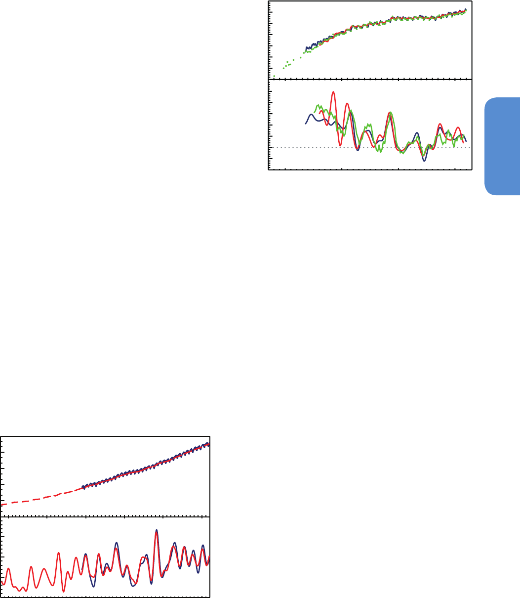
d(CO

)/dt (ppm yr

-1

)

(ppm)

380

360

340

320

(a)

(b)

1960 1970 1980 1990 2000 2010

Figure 2.1 | (a) Globally averaged CO

dry-air mole fractions from Scripps Institution

of Oceanography (SIO) at monthly time resolution based on measurements from Mauna

Loa, Hawaii and South Pole (red) and NOAA/ESRL/GMD at quasi-weekly time resolution

(blue). SIO values are deseasonalized. (b) Instantaneous growth rates for globally aver-

aged atmospheric CO

using the same colour code as in (a). Growth rates are calculated

as the time derivative of the deseasonalized global averages (Dlugokencky et al., 1994).

2009). Assuming no long-term trend in hydroxyl radical (OH) concen-

tration, the observed decrease in CH

growth rate from the early 1980s

through 2006 indicates an approach to steady state where total global

emissions have been approximately constant at ~550 Tg (CH

) yr

–1

Superimposed on the long-term pattern is signiﬁcant interannual vari-

ability; studies of this variability are used to improve understanding of

the global CH

budget (Chapter 6). The most likely drivers of increased

atmospheric CH

were anomalously high temperatures in the Arctic in

2007 and greater than average precipitation in the tropics during 2007

and 2008 (Dlugokencky et al., 2009; Bousquet, 2011). Observations of

the difference in CH

between zonal averages for northern and south-

ern polar regions (53° to 90°) (Dlugokencky et al., 2009, 2011) suggest

that, so far, it is unlikely that there has been a permanent measureable

increase in Arctic CH

emissions from wetlands and shallow sub-sea

clathrates.

Reaction with the hydroxyl radical (OH) is the main loss process for

(and for hydroﬂuorocarbons (HFCs) and hydrochloroﬂuorocarbons

(HCFCs)), and it is the largest term in the global CH

budget. Therefore,

trends and interannual variability in OH concentration signiﬁcantly

impact our understanding of changes in CH

emissions. Methyl chloro-

form (CH

CCl

; Section 2.2.1.2) has been used extensively to estimate

globally averaged OH concentrations (e.g., Prinn et al., 2005). AR4

reported no trend in OH from 1979 to 2004, and there is no evidence

from this assessment to change that conclusion for 2005 to 2011.

Montzka et al. (2011a) exploited the exponential decrease and small

emissions in CH

CCl

to show that interannual variations in OH con-

centration from 1998 to 2007 are 2.3 ± 1.5%, which is consistent with

estimates based on CH

, tetrachloroethene (C

), dichloromethane

(CH

), chloromethane (CH

Cl) and bromomethane (CH

Br).

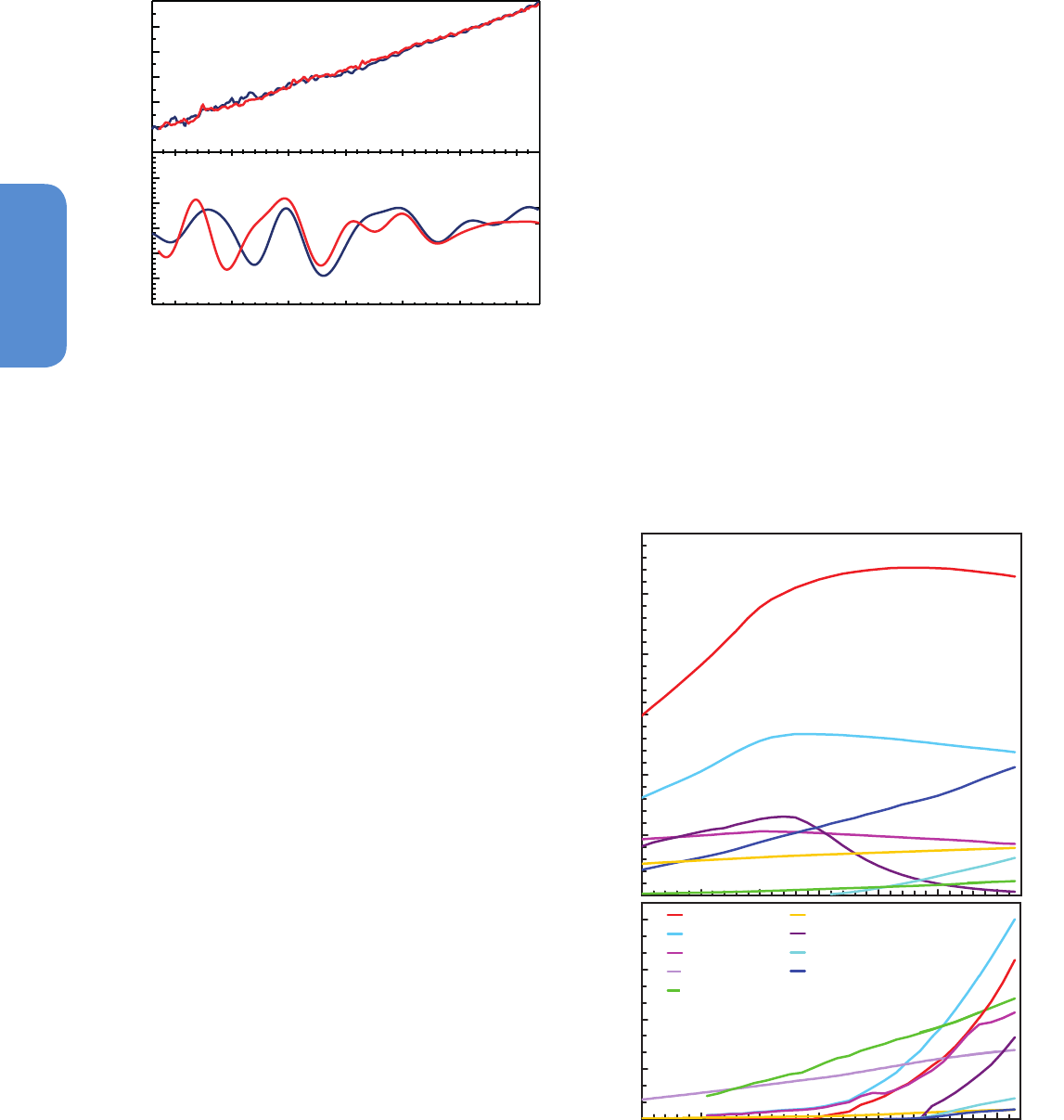
2.2.1.1.3 Nitrous Oxide

Globally averaged N

O in 2011 was 324.2 ppb, an increase of 5.0 ppb

over the value reported for 2005 in AR4 (Table 2.1). This is an increase

d(CH

)/dt (ppb yr

-1

)

(ppb)

1800

1750

1700

1650

1600

1550

-5

(a)

(b)

1980 1990

2000 2010

Figure 2.2 | (a) Globally averaged CH

dry-air mole fractions from UCI (green; four

values per year, except prior to 1984, when they are of lower and varying frequency),

AGAGE (red; monthly), and NOAA/ESRL/GMD (blue; quasi-weekly). (b) Instantaneous

growth rate for globally averaged atmospheric CH

using the same colour code as in (a).

Growth rates were calculated as in Figure 2.1.

168

Chapter 2 Observations: Atmosphere and Surface

of 20% over the estimate for 1750 from ice cores, 270 ± 7 ppb (Prather

et al., 2012). Measurements of N

O and its isotopic composition in ﬁrn

air suggest the increase, at least since the early 1950s, is dominated

by emissions from soils treated with synthetic and organic (manure)

nitrogen fertilizer (Rockmann and Levin, 2005; Ishijima et al., 2007;

Davidson, 2009; Syakila and Kroeze, 2011). Since systematic measure-

ments began in the late 1970s, N

O has increased at an average rate of

~0.75 ppb yr

–1

(Figure 2.3). Because the atmospheric burden of CFC-12

is decreasing, N

O has replaced CFC-12 as the third most important

well-mixed GHG contributing to RF (Elkins and Dutton, 2011).

Persistent latitudinal gradients in annually averaged N

O are observed

at background surface sites, with maxima in the northern subtropics,

values about 1.7 ppb lower in the Antarctic, and values about 0.4 ppb

lower in the Arctic (Huang et al., 2008). These persistent gradients

contain information about anthropogenic emissions from fertilizer use

at northern tropical to mid-latitudes and natural emissions from soils

and ocean upwelling regions of the tropics. N

O time series also con-

tain seasonal variations with peak-to-peak amplitudes of about 1 ppb

in high latitudes of the NH and about 0.4 ppb at high southern and

tropical latitudes. In the NH, exchange of air between the stratosphere

(where N

O is destroyed by photochemical processes) and troposphere

is the dominant contributor to observed seasonal cycles, not seasonali-

ty in emissions (Jiang et al., 2007). Nevison et al. (2011) found correla-

tions between the magnitude of detrended N

O seasonal minima and

lower stratospheric temperature, providing evidence for a stratospheric

inﬂuence on the timing and amplitude of the seasonal cycle at surface

monitoring sites. In the Southern Hemisphere (SH), observed seasonal

cycles are also affected by stratospheric inﬂux, and by ventilation and

thermal out-gassing of N

O from the oceans.

2.2.1.1.4 Hydroﬂuorocarbons, Perﬂuorocarbons, Sulphur

Hexaﬂuoride and Nitrogen Triﬂuoride

The budgets of HFCs, PFCs and SF

were recently reviewed in Chapter

1 of the Scientiﬁc Assessment of Ozone Depletion: 2010 (Montzka et

al., 2011b), so only a brief description is given here. The current atmos-

d(N

O)/dt (ppb yr

-1

O (ppb)

320

315

310

305

300

1.25

1.00

0.75

0.50

0.25

(a)

(b)

1980 1985 1990 1995 2000 20102005

Figure 2.3 | (a) Globally averaged N

O dry-air mole fractions from AGAGE (red) and

NOAA/ESRL/GMD (blue) at monthly resolution. (b) Instantaneous growth rates for glob-

ally averaged atmospheric N

O. Growth rates were calculated as in Figure 2.1.

pheric abundances of these species are summarized in Table 2.1 and

plotted in Figure 2.4.

Atmospheric HFC abundances are low and their contribution to RF is

small relative to that of the CFCs and HCFCs they replace (less than 1%

of the total by well-mixed GHGs; Chapter 8). As they replace CFCs and

HCFCs phased out by the Montreal Protocol, however, their contribu-

tion to future climate forcing is projected to grow considerably in the

absence of controls on global production (Velders et al., 2009).

HFC-134a is a replacement for CFC-12 in automobile air conditioners

and is also used in foam blowing applications. In 2011, it reached 62.7

ppt, an increase of 28.2 ppt since 2005. Based on analysis of high-fre-

quency measurements, the largest emissions occur in North America,

Europe and East Asia (Stohl et al., 2009).

HFC-23 is a by-product of HCFC-22 production. Direct measurements

of HFC-23 in ambient air at ﬁve sites began in 2007. The 2005 global

annual mean used to calculate the increase since AR4 in Table 2.1, 5.2

ppt, is based on an archive of air collected at Cape Grim, Tasmania

(Miller et al., 2010). In 2011, atmospheric HFC-23 was at 24.0 ppt. Its

growth rate peaked in 2006 as emissions from developing countries

Figure 2.4 | Globally averaged dry-air mole fractions at the Earth’s surface of the

major halogen-containing well-mixed GHG. These are derived mainly using monthly

mean measurements from the AGAGE and NOAA/ESRL/GMD networks. For clarity, only

the most abundant chemicals are shown in different compound classes and results from

different networks have been combined when both are available.

100

200

300

400

500

600

1980 1985 1990 1995 2000 2005 2010

Gas (ppt)

CFC-12

CCl

HCFC-22

CFC-11

HFC-23

HFC-134a

1980 1985 1990 1995 2000 2005 2010

Gas (ppt)

HFC-125

HFC-143a

HFC-152a

C2F6

SF6

C3F8

HFC-32

HFC-245fa

HFC-365mfc

169

Observations: Atmosphere and Surface Chapter 2

increased, then declined as emissions were reduced through abate-

ment efforts under the Clean Development Mechanism (CDM) of the

UNFCCC. Estimates of total global emissions based on atmospheric

observations and bottom-up inventories agree within uncertainties

(Miller et al., 2010; Montzka et al., 2010). Currently, the largest emis-

sions of HFC-23 are from East Asia (Yokouchi et al., 2006; Kim et al.,

2010; Stohl et al., 2010); developed countries emit less than 20% of the

global total. Keller et al. (2011) found that emissions from developed

countries may be larger than those reported to the UNFCCC, but their

contribution is small. The lifetime of HFC-23 was revised from 270 to

222 years since AR4.

After HFC-134a and HFC-23, the next most abundant HFCs are HFC-

143a at 12.04 ppt in 2011, 6.39 ppt greater than in 2005; HFC-125

(O’Doherty et al., 2009) at 9.58 ppt, increasing by 5.89 ppt since 2005;

HFC-152a (Greally et al., 2007) at 6.4 ppt with a 3.0 ppt increase since

2005; and HFC-32 at 4.92 ppt in 2011, 3.77 ppt greater than in 2005.

Since 2005, all of these were increasing exponentially except for HFC-

152a, whose growth rate slowed considerably in about 2007 (Figure

2.4). HFC-152a has a relatively short atmospheric lifetime of 1.5 years,

so its growth rate will respond quickly to changes in emissions. Its

major uses are as a foam blowing agent and aerosol spray propellant

while HFC-143a, HFC-125, and HFC-32 are mainly used in refriger-

ant blends. The reasons for slower growth in HFC-152a since about

2007 are unclear. Total global emissions of HFC-125 estimated from

the observations are within about 20% of emissions reported to the

UNFCCC, after accounting for estimates of unreported emissions from

East Asia (O’Doherty et al., 2009).

and C

(PFCs) have lifetimes of 50 kyr and 10 kyr, respective-

ly, and they are emitted as by-products of aluminium production and

used in plasma etching of electronics. CF

has a natural lithospheric

source (Deeds et al., 2008) with a 1750 level determined from Green-

land and Antarctic ﬁrn air of 34.7 ± 0.2 ppt (Worton et al., 2007; Muhle

et al., 2010). In 2011, atmospheric abundances were 79.0 ppt for CF

increasing by 4.0 ppt since 2005, and 4.16 ppt for C

, increasing by

0.50 ppt. The sum of emissions of CF

reported by aluminium produc-

ers and for non-aluminium production in EDGAR (Emission Database

for Global Atmospheric Research) v4.0 accounts for only about half

of global emissions inferred from atmospheric observations (Muhle et

al., 2010). For C

, emissions reported to the UNFCCC are also sub-

stantially lower than those estimated from atmospheric observations

(Muhle et al., 2010).

The main sources of atmospheric SF

emissions are electricity distri-

bution systems, magnesium production, and semi-conductor manufac-

turing. Global annual mean SF

in 2011 was 7.29 ppt, increasing by

1.65 ppt since 2005. SF

has a lifetime of 3200 years, so its emissions

accumulate in the atmosphere and can be estimated directly from its

observed rate of increase. Levin et al. (2010) and Rigby et al. (2010)

showed that SF

emissions decreased after 1995, most likely because

of emissions reductions in developed countries, but then increased

after 1998. During the past decade, they found that actual SF

emis-

sions from developed countries are at least twice the reported values.

was added to the list of GHG in the Kyoto Protocol with the Doha

Amendment, December, 2012. Arnold et al. (2013) determined 0.59 ppt

for its global annual mean mole fraction in 2008, growing from almost

zero in 1978. In 2011, NF

was 0.86 ppt, increasing by 0.49 ppt since

2005. These abundances were updated from the ﬁrst work to quantify

by Weiss et al. (2008). Initial bottom-up inventories underestimat-

ed its emissions; based on the atmospheric observations, NF

emissions

were 1.18 ± 0.21Gg in 2011 (Arnold et al., 2013).

In summary, it is certain that atmospheric burdens of well-mixed GHGs

targeted by the Kyoto Protocol increased from 2005 to 2011. The atmos-

pheric abundance of CO

was 390.5 ± 0.2 ppm in 2011; this is 40%

greater than before 1750. Atmospheric N

O was 324.2 ± 0.2 ppb in

2011 and has increased by 20% since 1750. Average annual increases

in CO

and N

O from 2005 to 2011 are comparable to those observed

from 1996 to 2005. Atmospheric CH

was 1803.2 ± 2.0 ppb in 2011; this

is 150% greater than before 1750. CH

began increasing in 2007 after

remaining nearly constant from 1999 to 2006. HFCs, PFCs, and SF

all

continue to increase relatively rapidly, but their contributions to RF are

less than 1% of the total by well-mixed GHGs (Chapter 8).

2.2.1.2 Ozone-Depleting Substances (Chloroﬂuorocarbons,

Chlorinated Solvents, and Hydrochloroﬂuorocarbons)

CFC atmospheric abundances are decreasing (Figure 2.4) because of the

successful reduction in emissions resulting from the Montreal Protocol.

By 2010, emissions from ODSs had been reduced by ~11 Pg CO

-eq

–1

, which is ﬁve to six times the reduction target of the ﬁrst com-

mitment period (2008–2012) of the Kyoto Protocol (2 PgCO

-eq yr

–1

)

(Velders et al., 2007). These avoided equivalent-CO

emissions account

for the offsets to RF by stratospheric O

depletion caused by ODSs and

the use of HFCs as substitutes for them. Recent observations in Arctic

and Antarctic ﬁrn air further conﬁrm that emissions of CFCs are entirely

anthropogenic (Martinerie et al., 2009; Montzka et al., 2011b). CFC-12

has the largest atmospheric abundance and GWP-weighted emissions

(which are based on a 100-year time horizon) of the CFCs. Its tropo-

spheric abundance peaked during 2000–2004. Since AR4, its global

annual mean mole fraction declined by 13.8 ppt to 528.5 ppt in 2011.

CFC-11 continued the decrease that started in the mid-1990s, by 12.9

ppt since 2005. In 2011, CFC-11 was 237.7 ppt. CFC-113 decreased by

4.3 ppt since 2005 to 74.3 ppt in 2011. A discrepancy exists between

top-down and bottom-up methods for calculating CFC-11 emissions

(Montzka et al., 2011b). Emissions calculated using top-down methods

come into agreement with bottom-up estimates when a lifetime of 64

years is used for CFC-11 in place of the accepted value of 45 years; this

longer lifetime (64 years) is at the upper end of the range estimated

by Douglass et al. (2008) with models that more accurately simulate

stratospheric circulation. Future emissions of CFCs will largely come

from ‘banks’ (i.e., material residing in existing equipment or stores)

rather than current production.

The mean decrease in globally, annually averaged carbon tetrachlo-

ride (CCl

) based on NOAA and AGAGE measurements since 2005 was

7.4 ppt, with an atmospheric abundance of 85.8 ppt in 2011 (Table

2.1). The observed rate of decrease and inter-hemispheric difference

of CCl

suggest that emissions determined from the observations are

on average greater and less variable than bottom-up emission esti-

mates, although large uncertainties in the CCl

lifetime result in large

uncertainties in the top-down estimates of emissions (Xiao et al., 2010;

170

Chapter 2 Observations: Atmosphere and Surface

Montzka et al., 2011b). CH

CCl

has declined exponentially for about a

decade, decreasing by 12.0 ppt since 2005 to 6.3 ppt in 2011.

HCFCs are classiﬁed as ‘transitional substitutes’ by the Montreal Proto-

col. Their global production and use will ultimately be phased out, but

their global production is not currently capped and, based on changes

in observed spatial gradients, there has likely been a shift in emissions

within the NH from regions north of about 30°N to regions south of

30°N (Montzka et al., 2009). Global levels of the three most abundant

HCFCs in the atmosphere continue to increase. HCFC-22 increased by

44.5 ppt since 2005 to 213.3 ppt in 2011. Developed country emissions

of HCFC-22 are decreasing, and the trend in total global emissions is

driven by large increases from south and Southeast Asia (Saikawa et

al., 2012). HCFC-141b increased by 3.7 ppt since 2005 to 21.4 ppt in

2011, and for HCFC-142b, the increase was 5.73 ppt to 21.1 ppt in

2011. The rates of increase in these three HCFCs increased since 2004,

but the change in HCFC-141b growth rate was smaller and less persis-

tent than for the other two, which approximately doubled from 2004

to 2007 (Montzka et al., 2009).

In summary, for ODS, whose production and consumption are con-

trolled by the Montreal Protocol, it is certain that the global mean

abundances of major CFCs are decreasing and HCFCs are increasing.

Atmospheric burdens of CFC-11, CFC-12, CFC-113, CCl

, CH

CCl

and

some halons have decreased since 2005. HCFCs, which are transitional

substitutes for CFCs, continue to increase, but the spatial distribution

of their emissions is changing.

2.2.2 Near-Term Climate Forcers

This section covers observed trends in stratospheric water vapour;

stratospheric and tropospheric ozone (O

); the O

precursor gases,

nitrogen dioxide (NO

) and carbon monoxide (CO); and column and

surface aerosol. Since trend estimates from the cited literature are used

here, issues such as data records of different length, potential lack of

comparability among measurement methods and different trend calcu-

lation methods, add to the uncertainty in assessing trends.

2.2.2.1 Stratospheric Water Vapour

Stratospheric H

O vapour has an important role in the Earth’s radi-

ative balance and in stratospheric chemistry. Increased stratospher-

ic H

O vapour causes the troposphere to warm and the stratosphere

to cool (Manabe and Strickler, 1964; Solomon et al., 2010), and also

causes increased rates of stratospheric O

loss (Stenke and Grewe,

2005). Water vapour enters the stratosphere through the cold tropical

tropopause. As moisture-rich air masses are transported through this

region, most water vapour condenses resulting in extremely dry lower

stratospheric air. Because tropopause temperature varies seasonally,

so does H

O abundance there. Other contributions include oxidation

of methane within the stratosphere, and possibly direct injection of

O vapour in overshooting deep convection (Schiller et al., 2009). AR4

reported that stratospheric H

O vapour showed signiﬁcant long-term

variability and an upward trend over the last half of the 20th century,

but no net increase since 1996. This updated assessment ﬁnds large

interannual variations that have been observed by independent meas-

urement techniques, but no signiﬁcant net changes since 1996.

The longest continuous time series of stratospheric water vapour abun-

dance is from in situ measurements made with frost point hygrome-

ters starting in 1980 over Boulder, USA (40°N, 105°W) (Scherer et al.,

2008), with values ranging from 3.5 to 5.5 ppm, depending on altitude.

These observations have been complemented by long-term global sat-

ellite observations from SAGE II (1984–2005; Stratospheric Aerosol

and Gas Experiment II (Chu et al., 1989)), HALOE (1991–2005; HAL-

ogen Occultation Experiment (Russell et al., 1993)), Aura MLS (2004–

present; Microwave Limb Sounder (Read et al., 2007)) and Envisat

MIPAS (2002-2012; Michelson Interferometer for Passive Atmospheric

Sounding (Milz et al., 2005; von Clarmann et al., 2009)). Discrepancies

in water vapour mixing ratios from these different instruments can be

attributed to differences in the vertical resolution of measurements,

along with other factors. For example, offsets of up to 0.5 ppm in lower

stratospheric water vapour mixing ratios exist between the most cur-

rent versions of HALOE (v19) and Aura MLS (v3.3) retrievals during

their 16-month period of overlap (2004 to 2005), although such biases

can be removed to generate long-term records. Since AR4, new studies

characterize the uncertainties in measurements from individual types

of in situ H

O sensors (Vömel et al., 2007b; Vömel et al., 2007a; Wein-

stock et al., 2009), but discrepancies between different instruments

(50 to 100% at H

O mixing ratios less than 10 ppm), particularly for

high-altitude measurements from aircraft, remain largely unexplained.

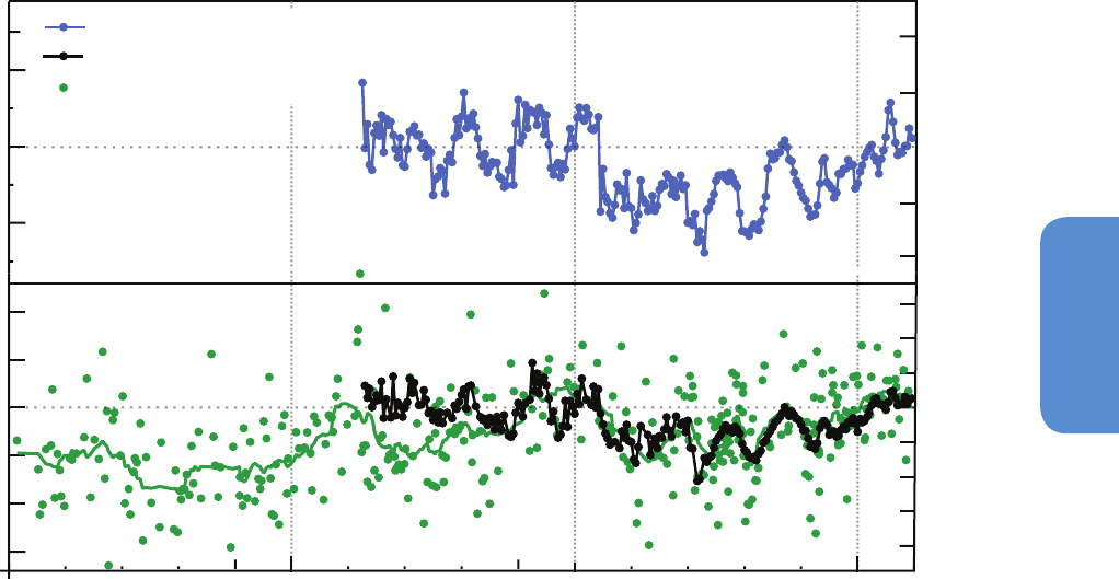
Observed anomalies in stratospheric H

O from the near-global com-

bined HALOE+MLS record (1992–2011) (Figure 2.5) include effects

linked to the stratospheric quasi-biennial oscillation (QBO) inﬂuence

on tropopause temperatures, plus a step-like drop after 2001 (noted in

AR4), and an increasing trend since 2005. Variability during 2001–2011

was large yet there was only a small net change from 1992 through

2011. These interannual water vapour variations for the satellite record

are closely linked to observed changes in tropical tropopause temper-

atures (Fueglistaler and Haynes, 2005; Randel et al., 2006; Rosenlof

and Reid, 2008; Randel, 2010), providing reasonable understanding of

observed changes. The longer record of Boulder balloon measurements

(since 1980) has been updated and reanalyzed (Scherer et al., 2008;

Hurst et al., 2011), showing deca dal-scale variability and a long-term

stratospheric (16 to 26 km) increase of 1.0 ± 0.2 ppm for 1980–2010.

Agreement between interannual changes inferred from the Boulder

and HALOE+MLS data is good for the period since 1998 but was poor

during 1992–1996. About 30% of the positive trend during 1980–2010

determined from frost point hygrometer data (Fujiwara et al., 2010;

Hurst et al., 2011) can be explained by increased production of H

from CH

oxidation (Rohs et al., 2006), but the remainder cannot be

explained by changes in tropical tropopause temperatures (Fueglistal-

er and Haynes, 2005) or other known factors.

In summary, near-global satellite measurements of stratospheric H

show substantial variability for 1992–2011, with a step-like decrease

after 2000 and increases since 2005. Because of this large variability

and relatively short time series, conﬁdence in long-term stratospher-

ic H

O trends is low. There is good understanding of the relationship

between the satellite-derived H

O variations and tropical tropopause

temperature changes. Stratospheric H

O changes from temporally

sparse balloon-borne observations at one location (Boulder, Colorado)

are in good agreement with satellite observations from 1998 to the

present, but discrepancies exist for changes during 1992–1996. Long-

171

Observations: Atmosphere and Surface Chapter 2

term balloon measurements from Boulder indicate a net increase of

1.0 ± 0.2 ppm over 16 to 26 km for 1980–2010, but these long-term

increases cannot be fully explained by changes in tropical tropopause

temperatures, methane oxidation or other known factors.

2.2.2.2 Stratospheric Ozone

AR4 did not explicitly discuss measured stratospheric ozone trends. For

the current assessment report such trends are relevant because they

are the basis for revising the RF from –0.05 ± 0.10 W m

–2

in 1750 to

–0.10 ± 0.15 W m

–2

in 2005 (Section 8.3.3.2). These values strongly

depend on the vertical distribution of the stratospheric ozone changes.

Total ozone is a good proxy for stratospheric ozone because tropo-

spheric ozone accounts for only about 10% of the total ozone column.

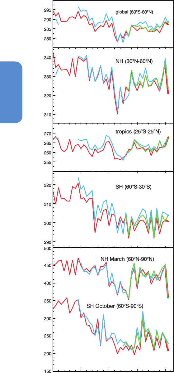
Long-term total ozone changes over various latitudinal belts, derived

from Weber et al. (2012), are illustrated in Figure 2.6 (a–d). Annual-

ly averaged total column ozone declined during the 1980s and early

1990s and has remained constant for the past decade, about 3.5 and

2.5% below the 1964–1980 average for the entire globe (not shown)

and 60°S to 60°N, respectively, with changes occurring mostly outside

the tropics, particularly the SH, where the current extratropical (30ºS

to 60ºS) mean values are 6% below the 1964–1980 average, com-

pared to 3.5% for the NH extratropics (Douglass et al., 2011). In the

NH, the 1993 minimum of about –6% was caused primarily by ozone

loss through heterogeneous reactions on volcanic aerosols from Mt.

Pinatubo.

0.5

0.0

-0.5

Water Vapour Anomaly (ppm)

-10

-20

Water Vapour

Anomaly (%)

HALOE+MLS: 60°S-60°N

-1.5

-1.0

-0.5

0.0

0.5

1.0

Water Vapour Anomaly (ppm)

2010200019901980

-40

-30

-20

-10

HALOE+MLS: 30°N-50°

NOAA FPH: Boulder (40°N)

(a)

(b)

Water Vapour

Anomaly (%)

Figure 2.5 | Water vapour anomalies in the lower stratosphere (~16 to 19 km) from satellite sensors and in situ measurements normalized to 2000–2011. (a) Monthly mean water

vapour anomalies at 83 hPa for 60°S to 60°N (blue) determined from HALOE and MLS satellite sensors. (b) Approximately monthly balloon-borne measurements of stratospheric

water vapour from Boulder, Colorado at 40°N (green dots; green curve is 15-point running mean) averaged over 16 to 18 km and monthly means as in (a), but averaged over 30°N

to 50°N (black)

Two altitude regions are mainly responsible for long-term changes in

total column ozone (Douglass et al., 2011). In the upper stratosphere

(35 to 45 km), there was a strong and statistically signiﬁcant decline

(about 10%) up to the mid-1990s and little change or a slight increase

since. The lower stratosphere, between 20 and 25 km over mid-lat-

itudes, also experienced a statistically signiﬁcant decline (7 to 8%)

between 1979 and the mid-1990s, followed by stabilization or a slight

(2 to 3%) ozone increase.

Springtime averages of total ozone poleward of 60° latitude in the

Arctic and Antarctic are shown in Figure 2.6e. By far the strongest

ozone loss in the stratosphere occurs in austral spring over Antarctica

(ozone hole) and its impact on SH climate is discussed in Chapters

11, 12 and 14. Interannual variability in polar stratospheric ozone

abundance and chemistry is driven by variability in temperature and

transport due to year-to-year differences in dynamics. This variability is

particularly large in the Arctic, where the most recent large depletion

occurred in 2011, when chemical ozone destruction was, for the ﬁrst

time in the observational record, comparable to that in the Antarctic

(Manney et al., 2011).

In summary, it is certain that global stratospheric ozone has declined

from pre-1980 values. Most of the decline occurred prior to the mid-

1990s; since then there has been little net change and ozone has

remained nearly constant at about 3.5% below the 1964–1980 level.

172

Chapter 2 Observations: Atmosphere and Surface

2.2.2.3 Tropospheric Ozone

Tropospheric ozone is a short-lived trace gas that either originates in

the stratosphere or is produced in situ by precursor gases and sunlight

(e.g., Monks et al., 2009). An important GHG with an estimated RF

of 0.40 ± 0.20 W m

–2

(Chapter 8), tropospheric ozone also impacts

human health and vegetation at the surface. Its average atmospheric

lifetime of a few weeks produces a global distribution highly variable

by season, altitude and location. These characteristics and the paucity

of long-term measurements make the assessment of long-term global

ozone trends challenging. However, new studies since AR4 provide

greater understanding of surface and free tropospheric ozone trends

from the 1950s through 2010. An extensive compilation of meas-

ured ozone trends is presented in the Supplementary Material, Figure

2.SM.1 and Table 2.SM.2.

The earliest (1876–1910) quantitative ozone observations are limited

to Montsouris near Paris where ozone averaged 11 ppb (Volz and Kley,

1988). Semiquantitative ozone measurements from more than 40 loca-

tions around the world in the late 1800s and early 1900s range from

5 to 32 ppb with large uncertainty (Pavelin et al., 1999). The low 19th

century ozone values cannot be reproduced by most models (Section

8.2.3.1), and this discrepancy is an important factor contributing to

uncertainty in RF calculations (Section 8.3.3.1). Limited quantitative

measurements from the 1870s to 1950s indicate that surface ozone in

Europe increased by more than a factor of 2 compared to observations

made at the end of the 20th century (Marenco et al., 1994; Parrish et

al., 2012).

Satellite-based tropospheric column ozone retrievals across the tropics

and mid-latitudes reveal a greater burden in the NH than in the SH

(Ziemke et al., 2011). Tropospheric column ozone trend analyses are

few. An analysis by Ziemke et al. (2005) found no trend over the trop-

ical Paciﬁc Ocean but signiﬁcant positive trends (5 to 9% per decade)

in the mid-latitude Paciﬁc of both hemispheres during 1979–2003. Sig-

niﬁcant positive trends (2 to 9% per decade) were found across broad

regions of the tropical South Atlantic, India, southern China, southeast

Asia, Indonesia and the tropical regions downwind of China (Beig and

Singh, 2007).

Long-term ozone trends at the surface and in the free troposphere (of

importance for calculating RF, Chapter 8) can be assessed only from

in situ measurements at a limited number of sites, leaving large areas

such as the tropics and SH sparsely sampled (Table 2.SM.2, Figure 2.7).

Nineteen predominantly rural surface sites or regions around the globe

have long-term records that stretch back to the 1970s, and in two

cases the 1950s (Lelieveld et al., 2004; Parrish et al., 2012; Oltmans et

al., 2013). Thirteen of these sites are in the NH, and 11 sites have statis-

tically signiﬁcant positive trends of 1 to 5 ppb per decade, correspond-

ing to >100% ozone increases since the 1950s and 9 to 55% ozone

increases since the 1970s. In the SH, three of six sites have signiﬁ-

cant trends of approximately 2 ppb per decade and three have insig-

niﬁcant trends. Free tropospheric monitoring since the 1970s is more

limited. Signiﬁcant positive trends since 1971 have been observed

using ozone sondes above Western Europe, Japan and coastal Antarc-

tica (rates of increase range from 1 to 3 ppb per decade), but not at

all levels (Oltmans et al., 2013). In addition, aircraft have measured

WOUDC (Brewer, Dobson, Filter)

GOME/SCIAMACHY/GOME2 (GSG)

BUV/TOMS/SBUV/OMI (MOD V8)

WOUDC (Brewer, Dobson, Filter)

GOME/SCIAMACHY/GOME2 (GSG)

BUV/TOMS/SBUV/OMI (MOD V8)

(DU) O

(DU)

1970 1980 1990 2000 2010

(a)

(b)

(c)

(d)

(e)

Figure 2.6 | Zonally averaged, annual mean total column ozone in Dobson Units

(DU; 1 DU = 2.69 × 10

/cm

) from ground-based measurements combining Brewer,

Dobson, and ﬁlter spectrometer data WOUDC (red), GOME/SCIAMACHY/GOME-2 GSG

(green) and merged satellite BUV/TOMS/SBUV/OMI MOD V8 (blue) for (a) Non-Polar

Global (60°S to 60°N), (b) NH (30°N to 60°N), (c) Tropics (25°S to 25°N), (d) SH (30°S

to 60°S) and (e) March NH Polar (60°N to 90°N) and October SH Polar. (Adapted from

Weber et al., 2012; see also for abbreviations.)

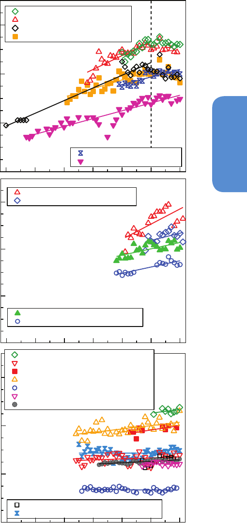
173

Observations: Atmosphere and Surface Chapter 2

signiﬁcant upper tropospheric trends in one or more seasons above

the north-eastern USA, the North Atlantic Ocean, Europe, the Middle

East, northern India, southern China and Japan (Schnadt Poberaj et

al., 2009). Insigniﬁcant free tropospheric trends were found above the

Mid-Atlantic USA (1971–2010) (Oltmans et al., 2013) and in the upper

troposphere above the western USA (1975–2001) (Schnadt Poberaj et

al., 2009). No site or region showed a signiﬁcant negative trend.

In recent decades ozone precursor emissions have decreased in Europe

and North America and increased in Asia (Granier et al., 2011), impact-

ing ozone production on regional and hemispheric scales (Skeie et al.,

2011). Accordingly, 1990–2010 surface ozone trends vary regionally. In

Europe ozone generally increased through much of the 1990s but since

2000 ozone has either levelled off or decreased at rural and mountain-

top sites, as well as for baseline ozone coming ashore at Mace Head,

Ireland (Tarasova et al., 2009; Logan et al., 2012; Parrish et al., 2012;

Oltmans et al., 2013). In North America surface ozone has increased in

eastern and Arctic Canada, but is unchanged in central and western

Canada (Oltmans et al., 2013). Surface ozone has increased in baseline

air masses coming ashore along the west coast of the USA (Parrish et

al., 2012) and at half of the rural sites in the western USA during spring

(Cooper et al., 2012). In the eastern USA surface ozone has decreased

strongly in summer, is largely unchanged in spring and has increased

in winter (Lefohn et al., 2010; Cooper et al., 2012). East Asian surface

ozone is generally increasing (Table 2.SM.2) and at downwind sites

ozone is increasing at Mauna Loa, Hawaii but decreasing at Minami

Tori Shima in the subtropical western North Paciﬁc (Oltmans et al.,

2013). In the SH ozone has increased at the eight available sites,

although trends are insigniﬁcant at four sites (Helmig et al., 2007; Olt-

mans et al., 2013).

Owing to methodological changes, free tropospheric ozone obser-

vations are most reliable since the mid-1990s. Ozone has decreased

above Europe since 1998 (Logan et al., 2012) and is largely unchanged

above Japan (Oltmans et al., 2013). Otherwise the remaining regions

with measurements (North America, North Paciﬁc Ocean, SH) show a

range of positive trends (both signiﬁcant and insigniﬁcant) depending

on altitude, with no site having a negative trend at any altitude (Table

2.SM.2).

In summary, there is medium conﬁdence from limited measurements

in the late 19th through mid-20th century that European surface ozone

more than doubled by the end of the 20th century. There is medium

conﬁdence from more widespread measurements beginning in the

1970s that surface ozone has increased at most (non-urban) sites in

the NH (1 to 5 ppb per decade), while there is low conﬁdence for ozone

increases (2 ppb per decade) in the SH. Since 1990 surface ozone has

likely increased in East Asia, while surface ozone in the eastern USA

and Western Europe has levelled off or is decreasing. Ozone monitor-

ing in the free troposphere since the 1970s is very limited and indicates

a weaker rate of increase than at the surface. Satellite instruments

can now quantify the present-day tropospheric ozone burden on a

near-global basis; signiﬁcant tropospheric ozone column increases

were observed over extended tropical regions of southern Asia, as well

as mid-latitude regions of the South and North Paciﬁc Ocean since

1979.

Jungfraujoch - 46ºN, 3.6 km

Zugspitze - 47ºN, 3.0 km

Arosa - 47ºN, 1.0 km

Hohenpeissenberg - 48ºN, 1.0 km

Mace Head - 55ºN, 0.2 km

Arkona-Zingst - 54ºN, 0.0 km

Mt. Happo - 36ºN, 1.9 km

Japanese MBL - 38-45ºN, ≤0.1 km

Lassen NP - 41ºN, 1.8 km

U.S. Pacific MBL - 38-48ºN, ≤0.2 km

Summit, Greenland - 72.6ºN, 3.2 km

Barrow, Alaska - 71.3ºN, 0.0 km

Storhofdi, Iceland - 63.3ºN, 1.0 km

Mauna Loa, Hawaii - 19.5ºN, 3.4 km

Samoa - 14.2ºS, 0.1 km

Cape Point, South Africa - 34.4ºS, 0.2 km

Cape Grim, Tasmania - 40.7ºS, 0.1 km

Arrival Heights, Antarctica - 77.8ºS, 0.1 km

South Pole- 90.0ºS, 2.8 km

Europe

Asia

North America

Other

latitudes

(ppb)O

(ppb)

1950 1960 1970 1980 1990 2000 2010

(a)

(b)

(c)

Figure 2.7 | Annual average surface ozone concentrations from regionally representa-

tive ozone monitoring sites around the world. (a) Europe. (b) Asia and North America.

legend is followed by its latitude and elevation. Time series include data from all times of

day and trend lines are linear regressions following the method of Parrish et al. (2012).

Trend lines are ﬁt through the full time series at each location, except for Jungfraujoch,

Zugspitze, Arosa and Hohenpeissenberg where the linear trends end in 2000 (indicated

by the dashed vertical line in (a)). Twelve of these 19 sites have signiﬁcant positive

ozone trends (i.e., a trend of zero lies outside the 95% conﬁdence interval); the seven

sites with non-signiﬁcant trends are: Japanese MBL (marine boundary layer), Summit

(Greenland), Barrow (Alaska), Storhofdi (Iceland), Samoa (tropical South Paciﬁc Ocean),

Cape Point (South Africa) and South Pole (Antarctica).

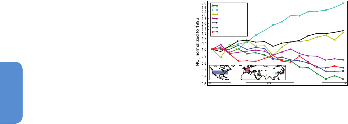
174

Chapter 2 Observations: Atmosphere and Surface

2.2.2.4 Carbon Monoxide, Non-Methane Volatile Organic

Compounds and Nitrogen Dioxide

Emissions of carbon monoxide (CO), non-methane volatile organic

compounds (NMVOCs) and NO

(NO + NO

) do not have a direct effect

on RF, but affect climate indirectly as precursors to tropospheric O

and aerosol formation, and their impacts on OH concentrations and

lifetime. NMVOCs include aliphatic, aromatic and oxygenated

hydrocarbons (e.g., aldehydes, alcohols and organic acids), and have

atmospheric lifetimes ranging from hours to months. Global cover-

age of NMVOC measurements is poor, except for a few compounds.

Reports on trends generally indicate declines in a range of NMVOCs

in urban and rural regions of North America and Europe on the order

of a few percent to more than 10% yr

–1

. Global ethane levels reported

by Simpson et al. (2012) declined by about 21% from 1986 to 2010.

Measurements of air extracted from ﬁrn suggest that NMVOC concen-

trations were growing until 1980 and declined afterwards (Aydin et al.,

2011; Worton et al., 2012). Satellite retrievals of formaldehyde column

abundances from 1997 to 2007 show signiﬁcant positive trends over

northeastern China (4% yr

–1

) and India (1.6% yr

–1

), possibly related to

strong increases in anthropogenic NMVOC emissions, whereas nega-

tive trends of about –3% yr

–1

are observed over Tokyo, Japan and the

northeast USA urban corridor as a result of pollution regulation (De

Smedt et al., 2010).

The major sources of atmospheric CO are in situ production by oxida-

tion of hydrocarbons (mostly CH

and isoprene) and direct emission

resulting from incomplete combustion of biomass and fossil fuels. An

analysis of MOPITT (Measurements of Pollutants in the Troposphere)

and AIRS (Atmospheric Infrared Sounder) satellite data suggesta clear

and consistent decline of CO columns for 2002–2010 over a number

of polluted regions in Europe, North America and Asia with a global

trend of about –1% yr

–1

(Yurganov et al., 2010; Fortems-Cheiney et al.,

2011; Worden et al., 2013). Analysis of satellite data using two more

instruments for recent overlapping years shows qualitatively similar

decreasing trends (Worden et al., 2013), but the magnitude of trends

remains uncertain owing to the presence of instrument biases. Small

CO decreases observed in the NOAA and AGAGE networks are consist-

ent with slight declines in global anthropogenic CO emissions over the

same time (Supplementary Material 2.SM.2).

Due to its short atmospheric lifetime (approximately hours), NO

con-

centrations are highly variable in time and space. AR4 described the

potential of satellite observations of NO

to verify and improve NO

emission inventories and their trends and reported strong NO

increas-

es by 50% over the industrial areas of China from 1996 to 2004. An

extension of this analysis reveals increases between a factor of 1.7

and 3.2 over parts of China, while over Europe and the USA NO

has

decreased by 30 to 50% between 1996 and 2010 (Hilboll et al., 2013).

Figure 2.8 shows the changes relative to 1996 in satellite-derived trop-

ospheric NO

columns, with a strong upward trend over central eastern

China and an overall downward trend in Japan, Europe and the USA.

reductions in the USA are very pronounced after 2004, related to

differences in effectiveness of NO

emission abatements in the USA and

also to changes in atmospheric chemistry of NO

(Russell et al., 2010).

Increasingly, satellite data are used to derive trends in anthropogenic

emissions, with Castellanos and Boersma (2012) reporting overall

increases in global emissions, driven by Asian emission increases of

up to 29% yr

–1

(1996–2006), while moderate decreases up to 7% yr

–1

(1996–2006) are reported for North America and Europe.

In summary, satellite and surface observations of ozone precursor

gases NO

, CO, and non-methane volatile organic carbons indicate

strong regional differences in trends. Most notably, NO

has likely

decreased by 30 to 50% in Europe and North America and increased

by more than a factor of 2 in Asia since the mid-1990s.

2.2.3 Aerosols

This section assesses trends in aerosol resulting from both anthro-

pogenic and natural sources. The signiﬁcance of aerosol changes for

global dimming and brightening is discussed in Section 2.3. Chapter 7

provides additional discussion of aerosol properties, while Chapter 8

discusses future RF and the ice-core records that contain information

on aerosol changes prior to the 1980s. Chapter 11 assesses air quali-

ty–climate change interactions. Because of the short lifetime (days to

weeks) of tropospheric aerosol, trends have a strong regional signa-

ture. Aerosol from anthropogenic sources (i.e., fossil and biofuel burn-

ing) are conﬁned mainly to populated regions in the NH, whereas aer-

osol from natural sources, such as desert dust, sea salt, volcanoes and

the biosphere, are important in both hemispheres and likely dependent

on climate and land use change (Carslaw et al., 2010). Owing to inter-

annual variability, long-term trends in aerosols from natural sources

are more difﬁcult to identify (Mahowald et al., 2010).

2.2.3.1 Aerosol Optical Depth from Remote Sensing

AOD is a measure of the integrated columnar aerosols load and is an

important parameter for evaluating aerosol–radiation interactions.

AR4 described early attempts to retrieve AOD from satellites but did

not provide estimates of temporal changes in tropospheric aerosol.

Little high-accuracy information on AOD changes exists prior to 1995.

Better satellite sensors and ground-based sun-photometer networks,

CE-U.S.

EC-China

NC-India

Japan

Middle East

cont. U.S.

W-Europe

1996 1998 2000 2002 2004 2006 2008 2010

GOME SCIAMACHY

Figure 2.8 | Relative changes in tropospheric NO

column amounts (logarithmic scale)

in seven selected world regions dominated by high NO

emissions. Values are normal-

ized for 1996 and derived from the GOME (Global Ozone Monitoring Experiment)

instrument from 1996 to 2002 and SCIAMACHY (Scanning Imaging Spectrometer for

Atmospheric Cartography) from 2003 to 2011 (Hilboll et al., 2013). The regions are

indicated in the map inset.

175

Observations: Atmosphere and Surface Chapter 2

along with improved retrieval methods and methodological intercom-

parisons, allow assessment of regional AOD trends since about 1995.

AOD sun photometer measurements at two stations in northern Ger-

many, with limited regional representativity, suggest a long-term

decline of AOD in Europe since 1986 (Ruckstuhl et al., 2008). Ground-

based, cloud-screened solar broadband radiometer measurements

provide longer time-records than spectrally selective sun-photometer

data, but are less speciﬁc for aerosol retrieval. Multi-decadal records

over Japan (Kudo et al., 2011) indicate an AOD increase until the mid-

1980s, followed by an AOD decrease until the late 1990s and almost

constant AOD in the 2000s. Similar broad-band solar radiative ﬂux

multi-decadal trends have been observed for urban–industrial regions

of Europe and North America (Wild et al., 2005), and were linked to

successful measures to reduce sulphate (precursor) emissions since the

mid-1980s (Section 2.3). An indirect method to estimate AOD is offered

by ground-based visibility observations. These data are more ambigu-

ous to interpret, but records go further back in time than broadband,

sun photometer and satellite data. A multi-regional analysis for 1973–

2007 (Wang et al., 2009a) shows that prior to the 1990s visibility-de-

rived AOD was relatively constant in most regions analysed (except for

positive trends in southern Asia), but after 1990 positive AOD trends

were observed over Asia, and parts of South America, Australia and

Africa, and mostly negative AOD trends were found over Europe. In

North America, a small stepwise decrease of visibility after 1993 was

likely related to methodological changes (Wang et al., 2012f).

AOD can be determined most accurately with sun photometers that

measure direct solar intensity in the absence of cloud interferences

with an absolute uncertainty of single measurements of ± 0.01%

(Holben et al., 1998). AERONET (AErosol RObotic NETwork) is a global

sun photometer network (Holben et al., 1998), with densest coverage

over Europe and North America. AERONET AOD temporal trends were

examined in independent studies (de Meij et al., 2012; Hsu et al., 2012;

Yoon et al., 2012), using different data selection and statistical meth-

ods. Hsu et al. (2012) investigated AOD trends at 12 AERONET sites

with data coverage of at least 10 years between 1997 and 2010. Yoon

et al. (2012) investigated AOD and size trends at 14 AERONET sites

with data coverage varying between 4 and 12 years between 1997

and 2009. DeMeij et al. (2012) investigated AOD trends between 2000

and 2009 (550 nm; monthly data) at 62 AERONET sites mostly located

in USA and Europe. Each of these studies noted an increase in AOD

over East Asia and reductions in North America and Europe. The only

dense sun photometer network over southern Asia, ARFINET (Aerosol

Radiative Forcing over India NETwork), shows an increase in AOD of

about 2% yr

–1

during the last one to two decades (Krishna Moorthy et

al., 2013), with an absolute uncertainty of ± 0.02 at 500 nm (Krishna

Moorthy et al., 2007). In contrast, negative AOD trends are identiﬁed at

more than 80% of examined European and North American AERONET

sites (de Meij et al., 2012). Decreasing AOD is also observed near the

west coast of northern Africa, where aerosol loads are dominated by

Saharan dust outﬂow. Positive AOD trends are found over the Arabi-

an Peninsula, where aerosol is dominated by dust. Inconsistent AOD

trends reported for stations in central Africa result from the use of rela-

tively short time series with respect to the large interannual variability

caused by wildﬁres and dust emissions.

Aerosol products from dedicated satellite sensors complement sur-

face-based AOD with better spatial coverage. The quality of the satel-

lite-derived AOD strongly depends on the retrieval’s ability to remove

scenes contaminated by clouds and to accurately account for reﬂectivi-

ty at the Earth’s surface. Due to relatively weak reﬂectance of incoming

sunlight by the sea surface, the typical accuracy of retrieved AOD over

oceans (uncertainty of 0.03 +0.05*AOD; Kahn et al. (2007)) is usually

better than over continents (uncertainty of 0.05 +0.15*AOD, Levy et

al. (2010)).

Satellite-based AOD trends at 550 nm over oceans from conservatively

cloud-screened MODIS data (Zhang and Reid, 2010) for 2000–2009 are

presented in Figure 2.9. Strongly positive AOD trends were observed

over the oceans adjacent to southern and eastern Asia. Positive AOD

trends are also observed over most tropical oceans. The negative

MODIS AOD trends observed over coastal regions of Europe and near

the east coast of the USA are in agreement with sun photometer obser-

vations and in situ measurements (Section 2.2.3.2) of aerosol mass

in these regions. These regional changes over oceans are consistent

with analyses of AVHRR (Advanced Very High Resolution Radiometer)

trends for 1981–2005 (Mishchenko et al., 2007; Cermak et al., 2010;

Zhao et al., 2011), except over the Southern Ocean (45°S to 60°S),

where negative AOD trends of AVHRR retrievals are neither conﬁrmed

by MODIS after 2001 (Zhang and Reid, 2010) nor by ATSR-2 (Along

Track Scanning Radiometer) for 1995–2001 (Thomas et al., 2010).

Satellite-based AOD changes for both land and oceans (Figure 2.9b)

were examined with re-processed SeaWiFS (Sea-viewing Wide Field-

of-view Sensor) AOD data for 1998–2010 (Hsu et al., 2012). A small

positive global average AOD trend is reported, which is likely inﬂu-

enced by interannual natural aerosol emissions variability (e.g., related

to ENSO or North Atlantic Oscillation (NAO); Box 2.5), and compen-

sating larger positive and negative regional AOD trends. In addition,

temporal changes in aerosol composition are ignored in the retrieval

algorithms, giving more uncertain trends than suggested by statisti-

cal analysis alone (Mishchenko et al., 2012). Thus, conﬁdence is low

for global satellite derived AOD trends over these relatively short time

periods.

The sign and magnitude of SeaWiFS regional AOD trends over conti-

nents are in agreement with most AOD trends by ground-based sun

photometer data (see above) and with MODIS trends (Figure 2.9). The

strong positive AOD trend over the Arabian Peninsula occurs mainly

during spring (MAM) and summer (JJA), during times of dust transport,

and is also visible in MODIS data (Figure 2.9). The positive AOD trend

over southern and eastern Asia is strongest during the dry seasons (DJF,

MAM), when reduced wet deposition allows anthropogenic aerosol to

accumulate in the troposphere. AOD over the Saharan outﬂow region

off western Africa displays the strongest seasonal AOD trend differ-

ences, with AOD increases only in spring, but strong AOD decreases

during the other seasons. SeaWifs AOD decreases over Europe and the

USA and increases over southern and eastern Asia (especially during

the dry season) are in agreement with reported temporal trends in

anthropogenic emissions, and surface observations (Section 2.2.3.2).

In summary, based on satellite- and surface-based remote sensing

it is very likely that AOD has decreased over Europe and the eastern

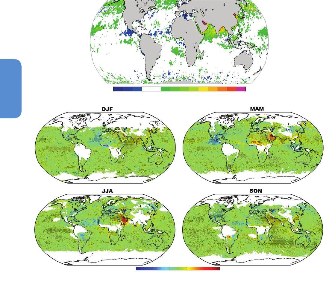
176

Chapter 2 Observations: Atmosphere and Surface

Aerosol Optical Depth trend (yr

-1

)

-0.04

-0.03

-0.02

-0.01

0.01

0.02

0.03

0.04

Aerosol Optical Depth trend x 100 (yr

-1

)

-1.2 -0.4 0

0.4

0.8

1.21.6

(a)

(b)

Figure 2.9 | (a) Annual average aerosol optical depth (AOD) trends at 0.55 μm for 2000–2009, based on de-seasonalized, conservatively cloud-screened MODIS aerosol data over

oceans (Zhang and Reid, 2010). Negative AOD trends off Mexico are due to enhanced volcanic activity at the beginning of the record. Most non-zero trends are signiﬁcant (i.e., a

trend of zero lies outside the 95% conﬁdence interval). (b) Seasonal average AOD trends at 0.55 μm for 1998–2010 using SeaWiFS data (Hsu et al., 2012). White areas indicate

incomplete or missing data. Black dots indicate signiﬁcant trends (i.e., a trend of zero lies outside the 95% conﬁdence interval).

USA since the mid 1990s and increased over eastern and southern

Asia since 2000. In the 2000s dust-related AOD has been increasing

over the Arabian Peninsula and decreasing over the North Atlantic

Ocean. Aerosol trends over other regions are less strong or not signiﬁ-

cant during this period owing to relative strong interannual variability.

Overall, conﬁdence in satellite-based global average AOD trends is low.

2.2.3.2 In Situ Surface Aerosol Measurements

AR4 did not report trends in long-term surface-based in situ meas-

urements of particulate matter, its components or its properties. This

section summarizes reported trends of PM

, PM

2.5

(particulate matter

with aerodynamic diameters <10 and <2.5 μm, respectively), sulphate

and equivalent black carbon/elemental carbon, from regionally repre-

sentative measurement networks. An overview of current networks

and deﬁnitions pertinent to aerosol measurements is given in Sup-

plementary Material 2.SM.2.3. Studies reporting trends representa-

tive of regional changes are presented in Table 2.2. Long-term data

are almost entirely from North America and Europe, whereas a few

individual studies on aerosol trends in India and China are reported

in Supplementary Material 2.SM.2.3. Figure 2.10 gives an overview

of observed PM

, PM

2.5

, and sulphate trends in North America and

Europe for 1990–2009 and 2000–2009.

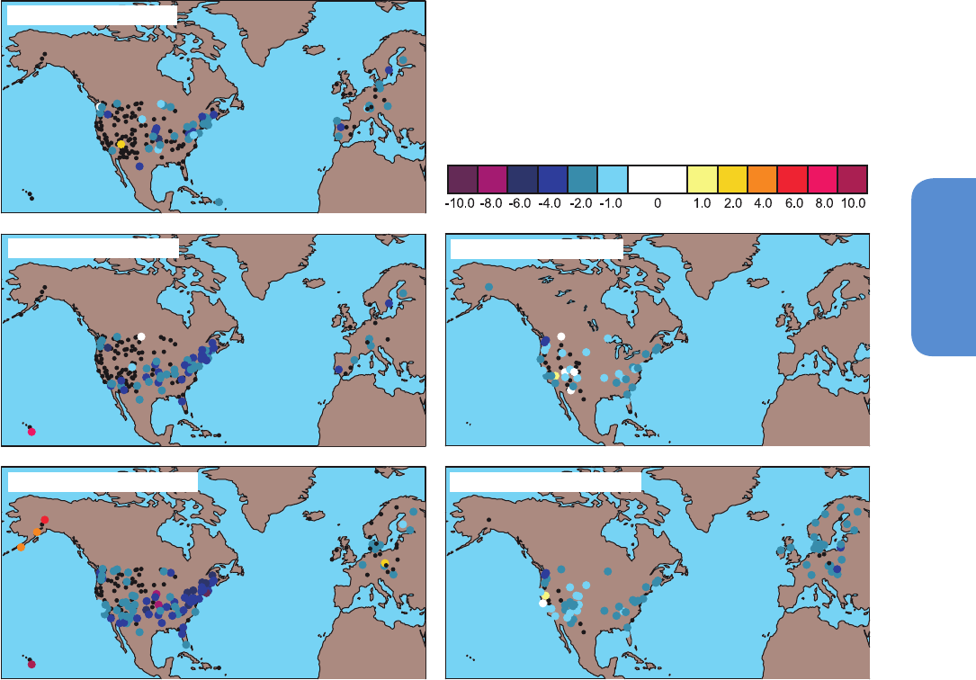
177

Observations: Atmosphere and Surface Chapter 2

In Europe, strong downward trends are observed for PM

, PM

2.5

and

sulphate from the rural stations in the EMEP (European Monitoring

and Evaluation Programme) network. For 2000–2009, PM

2.5

shows

an average reduction of 3.9% yr

–1

for the six stations with signiﬁcant

trends, while trends are not signiﬁcant at seven other stations. Over

2000–2009, PM

at 12 (out of 24) sites shows signiﬁcant downward

trend of on average 2.6% yr

–1

. Similarly sulphate strongly decreased

at 3.1% yr

–1

from 1990 to 2009 with 26 of 30 sites having signiﬁ-

cant reductions. The largest decrease occurred before 2000, while for

2000–2009, the trends were weaker and less robust. This is consistent

with reported emission reductions of 65% from 1990 to 2000 and 28%

from 2001 to 2009 (Yttri et al., 2011; Torseth et al., 2012). Model anal-

ysis (Pozzoli et al., 2011) attributed the trends in large part to emission

changes.

In the USA, the largest reductions in PM and sulphate are observed in

the 2000s, rather than the 1990s as in Europe. IMPROVE (U.S. Inter-

agency Monitoring of Protected Visual Environments Network) PM

2.5

measurements (Hand et al., 2011) show signiﬁcant downward trends

averaging 4.0% yr

–1

for 2000–2009 at sites with signiﬁcant trends,

(a) PM

, 2000-2009

(b) PM

2.5

, 2000-2009

(d) PM

2.5

, 1990-2009

Trend (% yr

-1

)

(e) Sulphate, 1990-2009

Figure 2.10 | Trends in particulate matter (PM

and PM

2.5

with aerodynamic diameters <10 and <2.5 μm, respectively) and sulphate in Europe and USA for two overlapping

periods 2000–2009 (a, b, c) and 1990–2009 (d, e). The trends are based on measurements from the EMEP (Torseth et al., 2012) and IMPROVE (Hand et al., 2011) networks in

Europe and USA, respectively. Sites with signiﬁcant trends (i.e., a trend of zero lies outside the 95% conﬁdence interval) are shown in colour; black dots indicate sites with non-

signiﬁcant trends.

and 2.1% yr

–1

at all sites, and PM

decreases of 3.1% yr

–1

for 2000–

2009. Declines of PM

2.5

and SO

2–

in Canada are very similar (Hidy and

Pennell, 2010), with annual mean PM

2.5

at urban measurement sites

decreasing by 3.6% yr

–1

during 1985–2006 (Canada, 2012).

In the eastern and southwestern USA, IMPROVE data show strong sul-

phate declines, which range from 2 to 6% yr

–1

, with an average of

2.3% yr

–1

for the sites with signiﬁcant negative trends for 1990–2009.

However, four IMPROVE sites show strong SO

2–

increases from 2000

to 2009, amounting to 11.9% yr

–1

, at Hawaii (1225 m above sea level),

and 4 to 7% yr

–1

at three sites in southwest Alaska.

A recent study on long-term trends in aerosol optical properties from

24 globally distributed background sites (Collaud Coen et al., 2013)

reported statistically signiﬁcant trends at 16 locations, but the sign and

magnitude of the trends varied largely with the aerosol property con-

sidered and geographical region (Table 2.3). Among the sites, this study

reported strong increases in absorption and scattering coefﬁcients in

the free troposphere at Mauna Loa, Hawaii (3400 m above sea level),

which is a regional feature also evident in the satellite-based AOD

178

Chapter 2 Observations: Atmosphere and Surface

Aerosol

variable

Trend, % yr

–1

(1σ,

standard deviation)

Period Reference Comments

Europe

2.5

–2.9 (1.31)

–3.9 (0.87)

2000–2009

(Adapted from Torseth et al., 2012)

Regional background sites

13 sites available, 6 sites show statistically signiﬁcant results. Average change was

–0.37 and –0.52

mg m

–3

–1

–1.9 (1.43)

–2.6 (1.19)

2000–2009

24 sites available, 12 sites show statistically signiﬁcant results. Average change was

–0.29 and –0.40

mg m

–3

–1

2–

–3.0 (0.82)

–3.1 (0.72)

1990–2009

30 sites available, 26 sites show statistically signiﬁcant results. Average change was

–0.04 and –0.04

mg m

–3

–1

2–

– 1.5 (1.41)

–2.0 (1.8)

2000–2009

30 sites available, 10 sites show statistically signiﬁcant results. Average change was

–0.01 and –0.01

mg m

–3

–1

–1.9 1991–2008

(Barmpadimos et al., 2012)

Rural and urban sites

10 sites in Switzerland. The trend is adjusted for change in meteorology—unadjusted

data did not differ strongly. The average change was –0.51 mg m

–3

–1

USA

2.5

–2.1 (2.08)

–4.0 (1.01)

2000–2009

Adapted from (Hand et al., 2011)

Regional background sites

153 sites available, 52 sites show statistically signiﬁcant negative results. Only 1 site

shows statisticallly positive trend.

2.5

–1.5 (1.25)

–2.1 (0.97)

1990–2009 153 sites available, 39 sites show statistically signiﬁcant results.

–1.7 (2.00)

–3.1 (1.65)

2000–2009 154 sites available, 37 sites show statistically signiﬁcant results.

2–

–3.0 (2.86)

–3.0 (0.62)

2000–2009

154 sites available, 83 sites show statistically signiﬁcant negative results. 4 sites

showed statistical positive trend.

2–

–2.0 (1.07)

–2.3 (0.85)

1990–2009 103 sites available, 41 sites show statistically signiﬁcant results.

Total Carbon –2.5 to –7.5 1989–2008

(Hand et al., 2011)

Regional background sites

The trend interval includes about 50 sites mainly located along the East and West

Coasts of the USA; fewer sites were situated in the central part of the continent.

Arctic

EBC

–3.8 (0.7)

1989–2008 (Hirdman et al., 2010) Alert, Canada 62.3°W 82.5°N

2–

–3.0 (0.6)

1985–2006

EBC

Not sig.

1998–2008 Barrow, Alaska, 156.6°W 71.3° N

2–

Not sig.

1997–2008

EBC

–9.0 (5.0)

2002–2009 Zeppelin, Svalbard, 11.9°E 78.9° N

2–

–1.9 (1.7)

1990–2008

Table 2.2 | Trend estimates for various aerosol variables reported in the literature, using data sets with at least 10 years of measurements. Unless otherwise noted, trends of indi-

vidual stations were reported in % yr

–1

, and 95% conﬁdence intervals. The standard deviation (in parentheses) is determined from the individual trends of a set of regional stations.

Notes:

Equivalent black carbon.

Trend numbers indicated refer to the subset of stations with signiﬁcant changes over time—generally in regions strongly inﬂuenced by anthropogenic emissions (Figure 2.10).

Trend values signiﬁcant at 1% level.

trends (illustrated in Figure 2.9). Possible explanations for these chang-

es include the inﬂuence of increasing Asian emissions and changes

in clouds and removal processes. More and longer Asian time series,

coupled with transport analyses, are needed to corroborate these ﬁnd-

ings. Aerosol number concentrations (Asmi et al., 2013) are declining

signiﬁcantly at most sites in Europe, North America, the Paciﬁc and the

Caribbean, but increasing at South Pole based on a study of 17 globally

distributed remote sites.

Total carbon (= light absorbing carbon + organic carbon) measure-

ments indicate highly signiﬁcant downward trends between 2.5 and

7.5% yr

–1

along the east and west coasts of the USA, and smaller and

less signiﬁcant trends in other regions of the USA from 1989 to 2008

(Hand et al., 2011; Murphy et al., 2011).

In Europe, Torseth et al. (2012) suggest a slight reduction in elemental

carbon concentrations at two stations from 2001 to 2009, subject to

large interannual variability. Collaud Coen et al. (2013) reported con-

sistent negative trends in the aerosol absorption coefﬁcient at stations

in the continental USA, Arctic and Antarctica, but mostly insigniﬁcant

trends in Europe over the last decade.

In the Arctic, changes in aerosol impact the atmosphere’s radiative bal-

ance as well as snow and ice albedo. Similar to Europe and the USA,

Hirdman et al. (2010) reported downward trends in equivalent black

carbon and SO

2–

for two out of total three Arctic stations and attribut-

ed them to emission changes.

In summary, declining AOD in Europe and North America is corrobo-

rated by very likely downward trends in ground-based in situ particu-

late matter measurements since the mid-1980s. Robust evidence from

around 200 regional background sites with in situ ground based aer-

osol measurements indicate downward trends in the last two decades

of PM

2.5

in parts of Europe (2 to 6% yr

–1

) and the USA (1 to 2.5% yr

–1

179

Observations: Atmosphere and Surface Chapter 2

Region

Trend, % yr

–1

(1σ,

standard deviation)

Period Reference Comments

Scattering coefﬁcient

Europe (4/1)

+0.6 (1.9)

+2.7

2001–2010

Adapted from (Collaud Coen et al.,

2013) Regional background sites

Trend study including 24 regional background sites with more than 10

years of observations. Regional averages for last 10 years are included

here. Values in parenthesis show total number of sites/number of sites with

signiﬁcant trend.

USA (14/10)

–2.0 (2.5)

–2.9 (2.4)

Mauna Loa (1/1) +2.7

Arctic (1/0) +2.4

Antarctica (1/0) +2.5

Absorption coefﬁcient

Europe (3/0) +0.3 (0.4)

2001–2010

Adapted from (Collaud Coen et al.,

2013) Regional background sites

Trend study of aerosol optical properties including 24 regional background

sites with more than 10 years of observations. Regional averages for last

10 years are included here. Values in parenthesis show total number of

sites and number of sites with signiﬁcant trend.

USA (1/1) –2.0

Mauna Loa (1/1) +9.0

Arctic (1/1) –6.5

Antarctica (1/1) –0.1

Particle number concentration

Europe (4/2)

–0.9 (1.8)

–2.3 (1.0)

2001–2010

Adapted from (Asmi et al., 2013)

Regional background sites

Trend study of particle number concentration (N) and size distribution

including 17 regional background sites. Regional averages of particle

number concentration for last 10 years are included here. Values in

parentheses show total number of sites and number of sites with

signiﬁcant trend.

North America and

Caribbean (3/3)

–5.3 (2.8)

–6.6 (1.1)

Mauna Loa (1/1) –3.5

Arctic (1/0) –1.3

Antarctica (2/2) +2.7 (1.4)

Table 2.3 | Summary table of aerosol optical property trends reported in the literature, using data sets with at least 10 years of measurements. Otherwise as in Table 2.2.

Box 2.2 | Quantifying Changes in the Mean: Trend Models and Estimation

Many statistical methods exist for estimating trends in environmental time series (see Chandler and Scott, 2011 for a review). The

assessment of long-term changes in historical climate data requires trend models that are transparent and robust, and that can provide

credible uncertainty estimates.

Linear Trends

Historical climate trends are frequently described and quantiﬁed by estimating the linear component of the change over time (e.g.,

AR4). Such linear trend modelling has broad acceptance and understanding based on its frequent and widespread use in the published

research assessed in this report, and its strengths and weaknesses are well known (von Storch and Zwiers, 1999; Wilks, 2006). Chal-

lenges exist in assessing the uncertainty in the trend and its dependence on the assumptions about the sampling distribution (Gaussian

or otherwise), uncertainty in the data, dependency models for the residuals about the trend line, and treating their serial correlation

(Von Storch, 1999; Santer et al., 2008).

The quantiﬁcation and visualization of temporal changes are assessed in this chapter using a linear trend model that allows for ﬁrst-

order autocorrelation in the residuals (Santer et al., 2008; Supplementary Material 2.SM.3). Trend slopes in such a model are the same as

ordinary least squares trends; uncertainties are computed using an approximate method. The 90% conﬁdence interval quoted is solely

that arising from sampling uncertainty in estimating the trend. Structural uncertainties, to the extent sampled, are apparent from the

range of estimates from different data sets. Parametric and other remaining uncertainties (Box 2.1), for which estimates are provided with

some data sets, are not included in the trend estimates shown here, so that the same method can be applied to all data sets considered.

Nonlinear Trends

There is no a priori physical reason why the long-term trend in climate variables should be linear in time. Climatic time series often

have trends for which a straight line is not a good approximation (e.g., Seidel and Lanzante, 2004). The residuals from a linear ﬁt in time

often do not follow a simple autoregressive or moving average process, and linear trend estimates can easily change when recalculated

(continued on next page)

Notes:

Trend numbers indicated refer to the subset of stations with signiﬁcant changes over time—generally in regions strongly inﬂuenced by anthropogenic emissions (Figure 2.10).

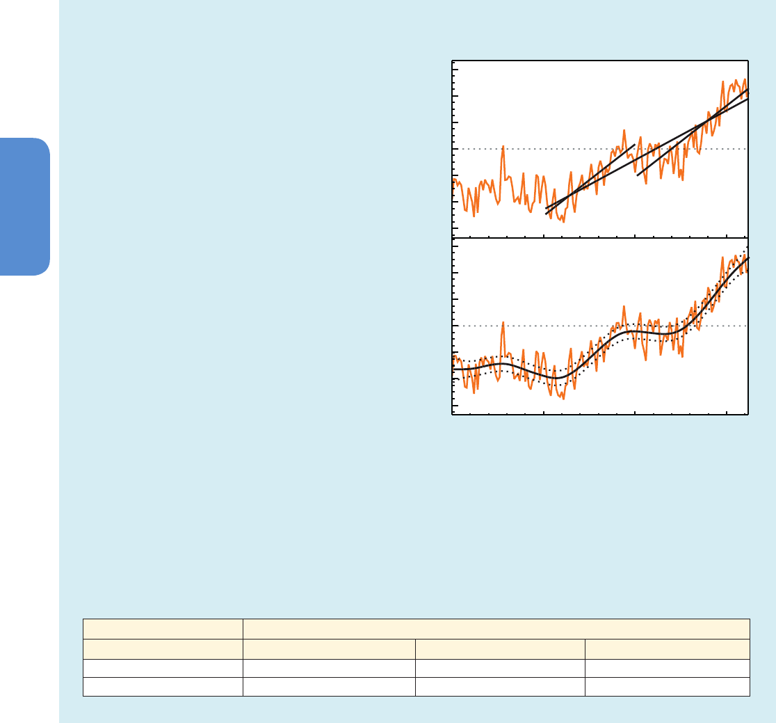
180

Chapter 2 Observations: Atmosphere and Surface

for shorter or longer time periods or when new data are

added. When linear trends for two parts of a longer time

series are calculated separately, the trends calculated for two

shorter periods may be very different (even in sign) from the

trend in the full period, if the time series exhibits signiﬁcant

nonlinear behavior in time (Box 2.2, Table 1).

Many methods have been developed for estimating the long-

term change in a time series without assuming that the change

is linear in time (e.g., Wu et al., 2007; Craigmile and Guttorp,

2011). Box 2.2, Figure 1 shows the linear least squares and

a nonlinear trend ﬁt to the GMST values from the HadCRUT4

data set (Section 2.4.3). The nonlinear trend is obtained by

ﬁtting a smoothing spline trend (Wood, 2006; Scinocca et

al., 2010) while allowing for ﬁrst-order autocorrelation in

the residuals (Supplementary Material 2.SM.3). The results

indicate that there are signiﬁcant departures from linearity

in the trend estimated this way.

Box 2.2, Table 1 shows estimates of the change in the GMST

from the two methods. The methods give similar estimates

with 90% conﬁdence intervals that overlap one another.

Smoothing methods that do not assume the trend is linear

can provide useful information on the structure of change

that is not as well treated with linear ﬁts. The linear trend ﬁt

is used in this chapter because it can be applied consistently

to all the data sets, is relatively simple, transparent and

easily comprehended, and is frequently used in the published

research assessed here.

and also for SO

2–

(2 to 5% yr

–1

). The strongest decreases were in the

1990s in Europe and in the 2000s in the USA. There is robust evidence

for downward trends of light absorbing aerosol in the USA and the

Arctic, while elsewhere in the world in situ time series are lacking or

not long enough to reach statistical signiﬁcance.

2.3 Changes in Radiation Budgets

The radiation budget of the Earth is a central element of the climate

system. On average, radiative processes warm the surface and cool the

atmosphere, which is balanced by the hydrological cycle and sensible

Box 2.2, Figure 1 | (a) Global mean surface temperature (GMST) anomalies relative

to a 1961–1990 climatology based on HadCRUT4 annual data. The straight black

lines are least squares trends for 1901–2012, 1901–1950 and 1951–2012. (b) Same

data as in (a), with smoothing spline (solid curve) and the 90% conﬁdence interval on

the smooth curve (dashed lines). Note that the (strongly overlapping) 90% conﬁdence

intervals for the least square lines in (a) are omitted for clarity. See Figure 2.20 for the

other two GMST data products.

0.6

0.4

0.2

0.0

-0.2

-0.4

-0.6

(a)

1850 1900

1950

2000

Temperature anomaly (ºC)

0.6

0.4

0.2

0.0

-0.2

-0.4

-0.6

(b)

Box 2.2 (continued)

heating. Spatial and temporal energy imbalances due to radiation and

latent heating produce the general circulation of the atmosphere and

oceans. Anthropogenic inﬂuence on climate occurs primarily through

perturbations of the components of the Earth radiation budget.

The radiation budget at the top of the atmosphere (TOA) includes the

absorption of solar radiation by the Earth, determined as the difference

between the incident and reﬂected solar radiation at the TOA, as well

as the thermal outgoing radiation emitted to space. The surface radia-

tion budget takes into account the solar ﬂuxes absorbed at the Earth’s

surface, as well as the upward and downward thermal radiative ﬂuxes

emitted by the surface and atmosphere, respectively. In view of new

Trends in °C per decade

Method 1901–2012 1901–1950 1951–2012

Least squares 0.075 ± 0.013 0.107 ± 0.026 0.106 ± 0.027

Smoothing spline 0.081 ± 0.010 0.070 ± 0.016 0.090 ± 0.018

Box 2.2, Table 1 | Estimates of the mean change in global mean surface temperature (GMST) between 1901 and 2012, 1901 and 1950, and 1951 and 2012,

obtained from the linear (least squares) and nonlinear (smoothing spline) trend models. Half-widths of the 90% conﬁdence intervals are also provided for the estimated

changes from the two trend methods.

181

Observations: Atmosphere and Surface Chapter 2

observational evidence since AR4, the mean state as well as multi-dec-

adal changes of the surface and TOA radiation budgets are assessed

in the following.

2.3.1 Global Mean Radiation Budget

Since AR4, knowledge on the magnitude of the radiative energy ﬂuxes

in the climate system has improved, requiring an update of the global

annual mean energy balance diagram (Figure 2.11). Energy exchanges

between Sun, Earth and Space are observed from space-borne plat-

forms such as the Clouds and the Earth’s Radiant Energy System (CERES,

Wielicki et al., 1996) and the Solar Radiation and Climate Experiment

(SORCE, Kopp and Lawrence, 2005) which began data collection in

2000 and 2003, respectively. The total solar irradiance (TSI) incident at

the TOA is now much better known, with the SORCE Total Irradiance

Monitor (TIM) instrument reporting uncertainties as low as 0.035%,

compared to 0.1% for other TSI instruments (Kopp et al., 2005). During

the 2008 solar minimum, SORCE/TIM observed a solar irradiance of

1360.8 ± 0.5 W m

–2

compared to 1365.5 ± 1.3 W m

–2

for instruments

launched prior to SORCE and still operating in 2008 (Section 8.4.1.1).

Kopp and Lean (2011) conclude that the SORCE/TIM value of TSI is the

most credible value because it is validated by a National Institute of

Standards and Technology calibrated cryogenic radiometer. This revised

TSI estimate corresponds to a solar irradiance close to 340 W m

–2

glob-

ally averaged over the Earth’s sphere (Figure 2.11).

100

(96, 100)

solar absorbed

surface

thermal

up surface

thermal

down surface

solar absorbed

atmosphere

thermal outgoing

TOA

evapo-

ration

sensible

heat

solar reflected

TOA

incoming

solar TOA

solar

reflected

surface

greenhouse

gases

atmospheric

window

latent heat

340

(340, 341)

161

(154, 166)

(74, 91)

239

(236, 242)

398

(394, 400)

342

(338, 348)

imbalance

(70, 85)

(15, 25)

(22,26)

solar

down

surface

185

(179, 189)

0.6

(0.2, 1.0)

Units (Wm

-2

)

Figure 2.11: | Global mean energy budget under present-day climate conditions. Numbers state magnitudes of the individual energy ﬂuxes in W m

–2

, adjusted within their

uncertainty ranges to close the energy budgets. Numbers in parentheses attached to the energy ﬂuxes cover the range of values in line with observational constraints. (Adapted

from Wild et al., 2013.)

The estimate for the reﬂected solar radiation at the TOA in Figure 2.11,

100 W m

–2

, is a rounded value based on the CERES Energy Balanced

and Filled (EBAF) satellite data product (Loeb et al., 2009, 2012b) for

the period 2001–2010. This data set adjusts the solar and thermal TOA

ﬂuxes within their range of uncertainty to be consistent with inde-

pendent estimates of the global heating rate based on in situ ocean

observations (Loeb et al., 2012b). This leaves 240 W m

–2

of solar radia-

tion absorbed by the Earth, which is nearly balanced by thermal emis-

sion to space of about 239 W m

–2

(based on CERES EBAF), considering

a global heat storage of 0.6 W m

–2

(imbalance term in Figure 2.11)

based on Argo data from 2005 to 2010 (Hansen et al., 2011; Loeb et

al., 2012b; Box 3.1). The stated uncertainty in the solar reﬂected TOA

ﬂuxes from CERES due to uncertainty in absolute calibration alone is

about 2% (2-sigma), or equivalently 2 W m

–2

(Loeb et al., 2009). The

uncertainty of the outgoing thermal ﬂux at the TOA as measured by

CERES due to calibration is ~3.7 W m

–2

(2σ). In addition to this, there is

uncertainty in removing the inﬂuence of instrument spectral response

on measured radiance, in radiance-to-ﬂux conversion, and in time–

space averaging, which adds up to another 1 W m

–2

(Loeb et al., 2009).

The components of the radiation budget at the surface are generally

more uncertain than their counterparts at the TOA because they cannot

be directly measured by passive satellite sensors and surface measure-

ments are not always regionally or globally representative. Since AR4,

new estimates for the downward thermal infrared (IR) radiation at

182

Chapter 2 Observations: Atmosphere and Surface

the surface have been established that incorporate critical information

on cloud base heights from space-borne radar and lidar instruments

(L’Ecuyer et al., 2008; Stephens et al., 2012a; Kato et al., 2013). In line

with studies based on direct surface radiation measurements (Wild et

al., 1998, 2013) these studies propose higher values of global mean

downward thermal radiation than presented in previous IPCC assess-

ments and typically found in climate models, exceeding 340 W m

–2

(Figure 2.11). This aligns with the downward thermal radiation in the

ERA-Interim and ERA-40 reanalyses (Box 2.3), of 341 and 344 W m

–2

respectively (Berrisford et al., 2011). Estimates of global mean down-

ward thermal radiation computed as a residual of the other terms of

the surface energy budget (Kiehl and Trenberth, 1997; Trenberth et al.,

2009) are lower (324 to 333 W m

–2

), highlighting remaining uncertain-

ties in estimates of both radiative and non-radiative components of the

surface energy budget.

Estimates of absorbed solar radiation at the Earth’s surface include

considerable uncertainty. Published global mean values inferred from

satellite retrievals, reanalyses and climate models range from below

160 W m

–2

to above 170 W m

–2

. Recent studies taking into account

surface observations as well as updated spectroscopic parameters

and continuum absorption for water vapor favour values towards

the lower bound of this range, near 160 W m

–2

, and an atmospheric

solar absorption around 80 W m

–2

(Figure 2.11) (Kim and Ramanathan,

2008; Trenberth et al., 2009; Kim and Ramanathan, 2012; Trenberth

and Fasullo, 2012b; Wild et al., 2013). The ERA-Interim and ERA-40

reanalyses further support an atmospheric solar absorption of this

magnitude (Berrisford et al., 2011). Latest satellite-derived estimates

constrained by CERES now also come close to these values (Kato et

al., in press). Recent independently derived surface radiation estimates

favour therefore a global mean surface absorbed solar ﬂux near 160

W m

–2

and a downward thermal ﬂux slightly above 340 W m

–2

, respec-

tively (Figure 2.11).

The global mean latent heat ﬂux is required to exceed 80 W m

–2

close the surface energy balance in Figure 2.11, and comes close to the

85 W m

–2

considered as upper limit by Trenberth and Fasullo (2012b)

in view of current uncertainties in precipitation retrieval in the Global

Precipitation Climatology Project (GPCP, Adler et al., 2012) (the latent

heat ﬂux corresponds to the energy equivalent of evaporation, which

globally equals precipitation; thus its magnitude may be constrained

by global precipitation estimates). This upper limit has recently been

challenged by Stephens et al. (2012b). The emerging debate reﬂects

potential remaining deﬁciencies in the quantiﬁcation of the radiative

and non-radiative energy balance components and associated uncer-

tainty ranges, as well as in the consistent representation of the global

mean energy and water budgets (Stephens et al., 2012b; Trenberth and

Fasullo, 2012b; Wild et al., 2013). Relative uncertainty in the globally

averaged sensible heat ﬂux estimate remains high owing to the very

limited direct observational constraints (Trenberth et al., 2009; Ste-

phens et al., 2012b).

In summary, newly available observations from both space-borne and

surface-based platforms allow a better quantiﬁcation of the Global

Energy Budget, even though notable uncertainties remain, particu-

larly in the estimation of the non-radiative surface energy balance

components.

2.3.2 Changes in Top of the Atmosphere Radiation

Budget

While the previous section emphasized the temporally-averaged state

of the radiation budget, the focus in the following is on the temporal

(multi-decadal) changes of its components. Variations in TSI are dis-

cussed in Section 8.4.1. AR4 reported large changes in tropical TOA

radiation between the 1980s and 1990s based on observations from

the Earth Radiation Budget Satellite (ERBS) (Wielicki et al., 2002;

Wong et al., 2006). Although the robust nature of the large decadal

changes in tropical radiation remains to be established, several studies

have suggested links to changes in atmospheric circulation (Allan and

Slingo, 2002; Chen et al., 2002; Clement and Soden, 2005; Merriﬁeld,

2011) (Section 2.7).

Since AR4, CERES enabled the extension of satellite records of TOA

ﬂuxes into the 2000s (Loeb et al., 2012b). The extended records from

CERES suggest no noticeable trends in either the tropical or global

radiation budget during the ﬁrst decade of the 21st century (e.g.,

Andronova et al., 2009; Harries and Belotti, 2010; Loeb et al., 2012a,

2012b). Comparisons between ERBS/CERES thermal radiation and that

derived from the NOAA High Resolution Infrared Radiation Sounder

(HIRS) (Lee et al., 2007) show good agreement until approximate-

ly 1998, corroborating the rise of 0.7 W m

–2

between the 1980s and

1990s reported in AR4. Thereafter the HIRS thermal ﬂuxes show much

higher values, likely due to changes in the channels used for HIRS/3

instruments launched after October 1998 compared to earlier HIRS

instruments (Lee et al., 2007).

On a global scale, interannual variations in net TOA radiation and

ocean heating rate (OHR) should correspond, as oceans have a much

larger effective heat capacity than land and atmosphere, and therefore

serve as the main reservoir for heat added to the Earth–atmosphere

system (Box 3.1). Wong et al. (2006) showed that interannual varia-

tions in these two data sources are in good agreement for 1992–2003.

In the ensuing 5 years, however, Trenberth and Fasullo (2010) note

that the two diverge with ocean in situ measurements (Levitus et al.,

2009), indicating a decline in OHR, in contrast to expectations from the

observed net TOA radiation. The divergence after 2004 is referred to as

‘‘missing energy’’ by Trenberth and Fasullo (2012b), who further argue

that the main sink of the missing energy likely occurs at ocean depths

below 275 m. Loeb et al. (2012b) compared interannual variations in

CERES net radiation with OHRs derived from three independent ocean

heat content anomaly analyses and included an error analysis of both

CERES and the OHRs. They conclude that the apparent decline in OHR

is not statistically robust and that differences between interannual var-

iations in OHR and satellite net TOA ﬂux are within the uncertainty

of the measurements (Figure 2.12). They further note that between

January 2001 and December 2012, the Earth has been steadily accu-

mulating energy at a rate of 0.50 ± 0.43 W m

–2

(90% CI). Hansen et al.

(2011) obtained a similar value for 2005–2010 using an independent

analysis of the ocean heat content anomaly data (von Schuckmann

and Le Traon, 2011). The variability in the Earth’s energy imbalance is

strongly inﬂuenced by ocean circulation changes relating to the ENSO

(Box 2.5); during cooler La Niña years (e.g., 2009) less thermal radia-

tion is emitted and the climate system gains heat while the reverse is

true for warmer El Niño years (e.g., 2010) (Figure 2.12).

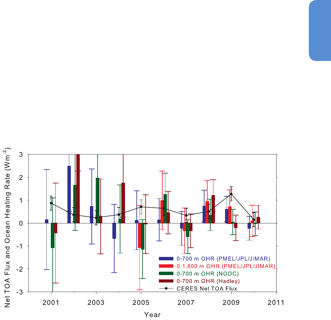
183

Observations: Atmosphere and Surface Chapter 2

In summary, satellite records of TOA radiation ﬂuxes have been sub-

stantially extended since AR4. It is unlikely that signiﬁcant trends exist

in global and tropical radiation budgets since 2000. Interannual vari-

ability in the Earth’s energy imbalance related to ENSO is consistent

with ocean heat content records within observational uncertainty.

2.3.3 Changes in Surface Radiation Budget

2.3.3.1 Surface Solar Radiation

Changes in radiative ﬂuxes at the surface can be traced further back

in time than the satellite-based TOA ﬂuxes, although only at selected

terrestrial locations where long-term records exist. Monitoring of radi-

ative ﬂuxes from land-based stations began on a widespread basis in

the mid-20th century, predominantly measuring the downward solar

component, also known as global radiation or surface solar radiation

(SSR).

AR4 reported on the ﬁrst indications for substantial decadal changes

in observational records of SSR. Speciﬁcally, a decline of SSR from the

beginning of widespread measurements in the 1950s until the mid-

1980s has been observed at many land-based sites (popularly known

as ‘global dimming’; Stanhill and Cohen, 2001; Liepert, 2002), as well

as a partial recovery from the 1980s onward (‘brightening’; Wild et al.,

2005) (see the longest available SSR series of Stockholm, Sweden, in

Figure 2.13 as an illustrative example).

Figure 2.12 | Comparison of net top of the atmosphere (TOA) ﬂux and upper ocean heating rates (OHRs). Global annual average (July to June) net TOA ﬂux from CERES observa-

tions (based on the EBAF-TOA_Ed2.6r product) (black line) and 0–700 (blue) and 0–1800 m (red) OHR from the Paciﬁc Marine Environmental Laboratory/Jet Propulsion Laboratory/

Joint Institute for Marine and Atmospheric Research (PMEL/JPL/JIMAR), 0–700 m OHR from the National Oceanic Data Center (NODC) (green; Levitus et al., 2009), and 0–700 m

OHR from the Hadley Center (brown; Palmer et al., 2007). The length of the coloured bars corresponds to the magnitude of OHR. Thin vertical lines are error bars, corresponding to

the magnitude of uncertainties. Uncertainties for all annual OHR are given at one standard error derived from ocean heat content anomaly uncertainties (Lyman et al., 2010). CERES

net TOA ﬂux uncertainties are given at the 90% conﬁdence level determined following Loeb et al. (2012b). (Adapted from Loeb et al., 2012b.)

Since AR4, numerous studies have substantiated the ﬁndings of sig-

niﬁcant decadal SSR changes observed both at worldwide distributed

terrestrial sites (Dutton et al., 2006; Wild et al., 2008; Gilgen et al.,

2009; Ohmura, 2009; Wild, 2009 and references therein) as well as in

speciﬁc regions. In Europe, Norris and Wild (2007) noted a dimming

between 1971 and 1986 of 2.0 to 3.1 W m

–2

per decade and subse-

quent brightening of 1.1 to 1.4 W m

–2

per decade from 1987 to 2002

in a pan-European time series comprising 75 sites. Similar tendencies

were found at sites in northern Europe (Stjern et al., 2009), Estonia

(Russak, 2009) and Moscow (Abakumova et al., 2008). Chiacchio and

Wild (2010) pointed out that dimming and subsequent brightening in

Europe is seen mainly in spring and summer. Brightening in Europe

from the 1980s onward was further documented at sites in Switzer-

land, Germany, France, the Benelux, Greece, Eastern Europe and the

Iberian Peninsula (Ruckstuhl et al., 2008; Wild et al., 2009; Zerefos et

al., 2009; Sanchez-Lorenzo et al., 2013). Concurrent brightening of 2

to 8 W m

–2

per decade was also noted at continental sites in the USA

(Long et al., 2009; Riihimaki et al., 2009; Augustine and Dutton, 2013).

The general pattern of dimming and consecutive brightening was fur-

ther found at numerous sites in Japan (Norris and Wild, 2009; Ohmura,

2009; Kudo et al., 2011) and in the SH in New Zealand (Liley, 2009).

Analyses of observations from sites in China conﬁrmed strong declines

in SSR from the 1960s to 1980s on the order of 2 to 8 W m

–2

per decade,

which also did not persist in the 1990s (Che et al., 2005; Liang and

Xia, 2005; Qian et al., 2006; Shi et al., 2008; Norris and Wild, 2009;

Xia, 2010a). On the other hand, persistent dimming since the mid-20th

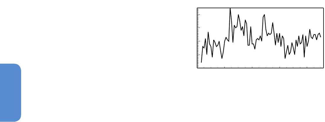
184

Chapter 2 Observations: Atmosphere and Surface

century with no evidence for a trend reversal was noted at sites in India

(Wild et al., 2005; Kumari et al., 2007; Kumari and Goswami, 2010;

Soni et al., 2012) and in the Canadian Prairie (Cutforth and Judiesch,

2007). Updates on latest SSR changes observed since 2000 provide

a less coherent picture (Wild, 2012). They suggest a continuation of

brightening at sites in Europe, USA, and parts of Asia, a levelling off at

sites in Japan and Antarctica, and indications for a renewed dimming

in parts of China (Wild et al., 2009; Xia, 2010a).

The longest observational SSR records, extending back to the 1920s

and 1930s at a few sites in Europe, further indicate some brightening

during the ﬁrst half of the 20th century, known as ‘early brightening’

(cf. Figure 2.13) (Ohmura, 2009; Wild, 2009). This suggests that the

decline in SSR, at least in Europe, was conﬁned to a period between

the 1950s and 1980s.

A number of issues remain, such as the quality and representativeness

of some of the SSR data as well as the large-scale signiﬁcance of the

phenomenon (Wild, 2012). The historic radiation records are of varia-

ble quality and rigorous quality control is necessary to avoid spurious

trends (Dutton et al., 2006; Shi et al., 2008; Gilgen et al., 2009; Tang

et al., 2011; Wang et al., 2012e; Sanchez-Lorenzo et al., 2013). Since

the mid-1990s, high-quality data are becoming increasingly available

from new sites of the Baseline Surface Radiation Network (BSRN) and

Atmospheric Radiation Measurement (ARM) Program, which allow the

determination of SSR variations with unprecedented accuracy (Ohmura

et al., 1998). Alpert et al. (2005) and Alpert and Kishcha (2008) argued

that the observed SSR decline between 1960 and 1990 was larger in

densely populated than in rural areas. The magnitude of this ‘urbani-

zation effect’ in the radiation data is not yet well quantiﬁed. Dimming

and brightening is, however, also notable at remote and rural sites

(Dutton et al., 2006; Karnieli et al., 2009; Liley, 2009; Russak, 2009;

Wild, 2009; Wang et al., 2012d).

Globally complete satellite estimates have been available since the

early 1980s (Hatzianastassiou et al., 2005; Pinker et al., 2005; Hin-

kelman et al., 2009). Because satellites do not directly measure the

surface ﬂuxes, they have to be inferred from measurable TOA signals

using empirical or physical models to remove atmospheric pertur-

bations. Available satellite-derived products qualitatively agree on a

brightening from the mid-1980s to 2000 averaged globally as well as

over oceans, on the order of 2 to 3 W m

–2

per decade (Hatzianastas-

siou et al., 2005; Pinker et al., 2005; Hinkelman et al., 2009). Averaged

over land, however, trends are positive or negative depending on the

respective satellite product (Wild, 2009). Knowledge of the decadal

variation of aerosol burdens and optical properties, required in satel-

lite retrievals of SSR and considered relevant for dimming/brightening

particularly over land, is very limited (Section 2.2.3). Extensions of sat-

ellite-derived SSR beyond 2000 indicate tendencies towards a renewed

dimming at the beginning of the new millennium (Hinkelman et al.,

2009; Hatzianastassiou et al., 2012).

Reconstructions of SSR changes from more widely measured mete-

orological variables can help to increase their spatial and temporal

coverage. Multi-decadal SSR changes have been related to observed

changes in sunshine duration, atmospheric visibility, diurnal tempera-

ture range (DTR; Section 2.4.1.2) and pan evaporation (Section 2.5.3).

Overall, these proxies provide independent evidence for the existence

of large-scale multi-decadal variations in SSR. Speciﬁcally, widespread

observations of declines in pan evaporation from the 1950s to the

1980s were related to SSR dimming amongst other factors (Roderick

and Farquhar, 2002). The observed decline in DTR over global land

surfaces from the 1950s to the 1980s (Section 2.4.1.2), and its stabi-

lisation thereafter ﬁts to a large-scale dimming and subsequent bright-

ening, respectively (Wild et al., 2007). Widespread brightening after

1980 is further supported by reconstructions from sunshine duration

records (Wang et al., 2012e). Over Europe, SSR dimming and subse-

quent brightening is consistent with concurrent declines and increas-

es in sunshine duration (Sanchez-Lorenzo et al., 2008), evaporation

in energy limited environments (Teuling et al., 2009), visibility records

(Vautard et al., 2009; Wang et al., 2009b) and DTR (Makowski et al.,

2009). The early brightening in the 1930s and 1940s seen in a few

European SSR records is in line with corresponding changes in sun-

shine duration and DTR (Sanchez-Lorenzo et al., 2008; Wild, 2009;

Sanchez-Lorenzo and Wild, 2012). In China, the levelling off in SSR in

the 1990s after decades of decline coincides with similar tendencies

in the pan evaporation records, sunshine duration and DTR (Liu et al.,

2004a; Liu et al., 2004b; Qian et al., 2006; Ding et al., 2007; Wang et al.,

2012d). Dimming up to the 1980s and subsequent brightening is also

indicated in a set of 237 sunshine duration records in South America

(Raichijk, 2011).

2.3.3.2 Surface Thermal and Net Radiation

Thermal radiation, also known as longwave, terrestrial or far-IR radi-

ation is sensitive to changes in atmospheric GHGs, temperature and

humidity. Long-term measurements of the thermal surface com-

ponents as well as surface net radiation are available at far fewer

sites than SSR. Downward thermal radiation observations started to

become available during the early 1990s at a limited number of glob-

ally distributed terrestrial sites. From these records, Wild et al. (2008)

determined an overall increase of 2.6 W m

–2

per decade over the 1990s,

in line with model projections and the expectations of an increasing

greenhouse effect. Wang and Liang (2009) inferred an increase in

downward thermal radiation of 2.2 W m

–2

per decade over the period

1973–2008 from globally available terrestrial observations of temper-

ature, humidity and cloud fraction. Prata (2008) estimated a slightly

lower increase of 1.7 W m

–2

per decade for clear sky conditions over

the earlier period 1964–1990, based on observed temperature and

1940 1960 1980 2000

Radiation (Wm

-2

)

100

110

120

130

1920

Figure 2.13 | Annual mean Surface Solar Radiation (SSR) as observed at Stockholm,

Sweden, from 1923 to 2010. Stockholm has the longest SSR record available world-

wide. (Updated from Wild (2009) and Ohmura (2009).)

185

Observations: Atmosphere and Surface Chapter 2

humidity proﬁles from globally distributed land-based radiosonde sta-

tions and radiative transfer calculations. Philipona et al. (2004; 2005)

and Wacker et al. (2011) noted increasing downward thermal ﬂuxes

recorded in the Swiss Alpine Surface Radiation Budget (ASRB) network

since the mid-1990s, corroborating an increasing greenhouse effect.

For mainland Europe, Philipona et al. (2009) estimated an increase of

downward thermal radiation of 2.4 to 2.7 W m

–2

per decade for the

period 1981–2005.

There is limited observational information on changes in surface net

radiation, in large part because measurements of upward ﬂuxes at the

surface are made at only a few sites and are not spatially representa-

tive. Wild et al. (2004, 2008) inferred a decline in land surface net radi-

ation on the order of 2 W m

–2

per decade from the 1960s to the 1980s,

and an increase at a similar rate from the 1980s to 2000, based on esti-

mated changes of the individual radiative components that constitute

the surface net radiation. Philipona et al. (2009) estimated an increase

in surface net radiation of 1.3 to 2 W m

–2

per decade for central Europe

and the Alps between 1981 and 2005.

2.3.3.3 Implications from Observed Changes in Related

Climate Elements

The observed multi-decadal SSR variations cannot be explained by

changes in TSI, which are an order of magnitude smaller (Willson and

Mordvinov, 2003). They therefore have to originate from alterations

in the transparency of the atmosphere, which depends on the pres-

ence of clouds, aerosols and radiatively active gases (Kvalevag and

Myhre, 2007; Kim and Ramanathan, 2008). Cloud cover changes (Sec-

tion 2.5.7) effectively modulate SSR on an interannual basis, but their

contribution to the longer-term SSR trends is ambiguous. Although

cloud cover changes were found to explain the trends in some areas

(e.g., Liley, 2009), this is not always the case, particularly in relatively

polluted regions (Qian et al., 2006; Norris and Wild, 2007, 2009; Wild,

2009; Kudo et al., 2012). SSR dimming and brightening has also been

observed under cloudless atmospheres at various locations, pointing to

a prominent role of atmospheric aerosols (Wild et al., 2005; Qian et al.,

2007; Ruckstuhl et al., 2008; Sanchez-Lorenzo et al., 2009; Wang et al.,

2009b; Zerefos et al., 2009).

Box 2.3 | Global Atmospheric Reanalyses

Dynamical reanalyses are increasingly used for assessing weather and climate phenomena. Given their more frequent use in this

assessment compared to AR4, their characteristics are described in more detail here.

Reanalyses are distinct from, but complement, more ‘traditional’ statistical approaches to assessing the raw observations. They aim to

produce continuous reconstructions of past atmospheric states that are consistent with all observations as well as with atmospheric

physics as represented in a numerical weather prediction model, a process termed data assimilation. Unlike real-world observations,

reanalyses are uniform in space and time and provide non-observable variables (e.g., potential vorticity).

Several groups are actively pursuing reanalysis development at the global scale, and many of these have produced several generations

of reanalyses products (Box 2.3, Table 1). Since the ﬁrst generation of reanalyses produced in the 1990s, substantial development has

taken place. The NASA Modern-Era Retrospective Analysis for Research and Applications (MERRA) and ERA-Interim reanalyses show

improved tropical precipitation and hence better represent the global hydrological cycle (Dee et al., 2011b). The NCEP/CFSR reanalysis

(continued on next page)

Institution Reanalysis Period

Approximate Resolution

at Equator

Reference

Cooperative Institute for Research in Environmental Sciences (CIRES),

National Oceanic and Atmospheric Administration (NOAA), USA

20th Century Reanalysis,

Vers. 2 (20CR)

1871–2010 320 km Compo et al. (2011)

National Centers for Environmental Prediction (NCEP) and National

Center for Atmospheric Research (NCAR), USA

NCEP/NCAR R1 (NNR) 1948– 320 km Kistler et al. (2001)

European Centre for Medium-Range Weather Forecasts (ECMWF) ERA-40 1957–2002 125 km Uppala et al. (2005)

Japan Meteorological Agency (JMA) JRA-55 1958– 60 km Ebita et al. (2011)

National Centers for Environmental Prediction (NCEP), US Department

of Energy, USA

NCEP/DOE R2 1979– 320 km Kanamitsu et al. (2002)

Japan Meteorological Agency (JMA) JRA-25 1979– 190 km Onogi et al. (2007)

National Aeronautics and Space Administration (NASA), USA MERRA 1979– 75 km Rienecker et al. (2011)

European Centre for Medium-Range Weather Forecasts (ECMWF) ERA-Interim 1979– 80 km Dee et al. (2011b)

National Centers for Environmental Prediction (NCEP), USA CFSR 1979– 50 km Saha et al. (2010)

Box 2.3, Table 1 | Overview of global dynamical reanalysis data sets (ranked by start year; the period extends to present if no end year is provided). A further

description of reanalyses and their technical derivation is given in pp. S33–35 of Blunden et al. (2011). Approximate resolution is calculated as 1000 km * 20/N

(with N denoting the spectral truncation, Laprise, 1992).

186

Chapter 2 Observations: Atmosphere and Surface

Aerosols can directly attenuate SSR by scattering and absorbing solar

radiation, or indirectly, through their ability to act as cloud condensa-

tion nuclei, thereby changing cloud reﬂectivity and lifetime (Chapter

7). SSR dimming and brightening is often reconcilable with trends in

anthropogenic emission histories and atmospheric aerosol loadings

(Stern, 2006; Streets et al., 2006; Mishchenko et al., 2007; Ruckstuhl et

al., 2008; Ohvril et al., 2009; Russak, 2009; Streets et al., 2009; Cermak

et al., 2010; Wild, 2012). Recent trends in aerosol optical depth derived

from satellites indicate a decline in Europe since 2000 (Section 2.2.3),

in line with evidence from SSR observations. However, direct aerosol

effects alone may not be able to account for the full extent of the

observed SSR changes in remote regions with low pollution levels

(Dutton and Bodhaine, 2001; Schwartz, 2005). Aerosol indirect effects

have not yet been well quantiﬁed, but have the potential to amplify

aerosol-induced SSR trends, particularly in relatively pristine environ-

ments, such as over oceans (Wild, 2012).

SSR trends are also qualitatively in line with observed multi-decadal

surface warming trends (Chapter 10), with generally smaller warm-

ing rates during phases of declining SSR, and larger warming rates

in phases of increasing SSR (Wild et al., 2007). This is seen more pro-

nounced for the relatively polluted NH than the more pristine SH (Wild,

2012). For Europe, Vautard et al. (2009) found that a decline in the fre-

quency of low-visibility conditions such as fog, mist and haze over the

past 30 years and associated SSR increase may be responsible for 10

to 20% of Europe’s recent daytime warming, and 50% of Eastern Euro-

pean warming. Philipona (2012) noted that both warming and bright-

ening are weaker in the European Alps compared to the surrounding

lowlands with stronger aerosol declines since 1981.

Reanalyses and observationally based methods have been used to

show that increased atmospheric moisture with warming (Willett et

al., 2008; Section 2.5) enhances thermal radiative emission of the

atmosphere to the surface, leading to reduced net thermal cooling of

the surface (Prata, 2008; Allan, 2009; Philipona et al., 2009; Wang and

Liang, 2009).

In summary, the evidence for widespread multi-decadal variations in

solar radiation incident on land surfaces has been substantiated since

AR4, with many of the observational records showing a decline from

the 1950s to the 1980s (‘dimming’), and a partial recovery thereafter

(‘brightening’). Conﬁdence in these changes is high in regions with

high station densities such as over Europe and parts of Asia. These

likely changes are generally supported by observed changes in related,

but more widely measured variables, such as sunshine duration, DTR

and hydrological quantities, and are often in line with aerosol emission

patterns. Over some remote land areas and over the oceans, conﬁ-

dence is low owing to the lack of direct observations, which hamper a

truly global assessment. Satellite-derived SSR ﬂuxes support the exist-

ence of brightening also over oceans, but are less consistent over land

surface where direct aerosol effects become more important. There are

also indications for increasing downward thermal and net radiation

at terrestrial stations since the early 1990s with medium conﬁdence.

uses a coupled ocean–atmosphere–land-sea–ice model (Saha et al., 2010). The 20th Century Reanalyses (20CR, Compo et al., 2011) is a

56-member ensemble and covers 140 years by assimilating only surface and sea level pressure (SLP) information. This variety of groups

and approaches provides some indication of the robustness of reanalyses when compared. In addition to the global reanalyses, several

regional reanalyses exist or are currently being produced.

Reanalyses products provide invaluable information on time scales ranging from daily to interannual variability. However, they may

often be unable to characterize long-term trends (Trenberth et al., 2011). Although reanalyses projects by deﬁnition use a ‘frozen’

assimilation system, there are many other sources of potential errors. In addition to model biases, changes in the observational systems

(e.g., coverage, introduction of satellite data) and time-dependent errors in the underlying observations or in the boundary conditions

lead to step changes in time, even in latest generation reanalyses (Bosilovich et al., 2011).

Errors of this sort were ubiquitous in early generation reanalyses and rendered them of limited value for trend characterization (Thorne

and Vose, 2010). Subsequent products have improved and uncertainties are better understood (Dee et al., 2011a), but artefacts are

still present. As a consequence, trend adequacy depends on the variable under consideration, the time period and the region of inter-

est. For example, surface air temperature and humidity trends over land in the ERA-Interim reanalysis compare well with observations

(Simmons et al., 2010), but polar tropospheric temperature trends in ERA-40 disagree with trends derived from radiosonde and satel-

lite observations (Bitz and Fu, 2008; Grant et al., 2008; Graversen et al., 2008; Thorne, 2008; Screen and Simmonds, 2011) owing to

problems that were resolved in ERA-Interim (Dee et al., 2011a).

Studies based on reanalyses are used cautiously in AR5 and known inadequacies are pointed out and referenced. Later generation

reanalyses are preferred where possible; however, literature based on these new products is still sparse.

Box 2.3 (continued)

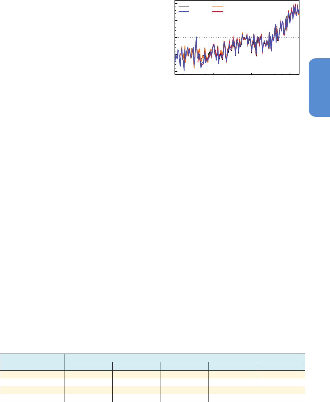
187

Observations: Atmosphere and Surface Chapter 2

Particular controversy since AR4 has surrounded the LSAT record over

the United States, focussed on siting quality of stations in the US His-

torical Climatology Network (USHCN) and implications for long-term

trends. Most sites exhibit poor current siting as assessed against ofﬁ-

cial WMO siting guidance, and may be expected to suffer potentially

large siting-induced absolute biases (Fall et al., 2011). However, overall

biases for the network since the 1980s are likely dominated by instru-

ment type (owing to replacement of Stevenson screens with maximum

minimum temperature systems (MMTS) in the 1980s at the majori-

ty of sites), rather than siting biases (Menne et al., 2010; Williams et

al., 2012). A new automated homogeneity assessment approach (also

used in GHCNv3, Menne and Williams, 2009) was developed that has

been shown to perform as well or better than other contemporary

approaches (Venema et al., 2012). This homogenization procedure

likely removes much of the bias related to the network-wide changes

in the 1980s (Menne et al., 2010; Fall et al., 2011; Williams et al., 2012).

Williams et al. (2012) produced an ensemble of data set realizations

using perturbed settings of this procedure and concluded through

assessment against plausible test cases that there existed a propensity

to under-estimate adjustments. This propensity is critically dependent

upon the (unknown) nature of the inhomogeneities in the raw data

records. Their homogenization increases both minimum temperature

and maximum temperature centennial-time-scale USA average LSAT

trends. Since 1979 these adjusted data agree with a range of reanalysis

products whereas the raw records do not (Fall et al., 2010; Vose et al.,

2012a).

Regional analyses of LSAT have not been limited to the United States.

Various national and regional studies have undertaken assessments for

Europe (Winkler, 2009; Bohm et al., 2010; Tietavainen et al., 2010; van

2.4 Changes in Temperature

2.4.1 Land Surface Air Temperature

2.4.1.1 Large-Scale Records and Their Uncertainties

AR4 concluded global land-surface air temperature (LSAT) had

increased over the instrumental period of record, with the warming

rate approximately double that reported over the oceans since 1979.

Since AR4, substantial developments have occurred including the pro-

duction of revised data sets, more digital data records, and new data

set efforts. These innovations have improved understanding of data

issues and uncertainties, allowing better quantiﬁcation of regional

changes. This reinforces conﬁdence in the reported globally averaged

LSAT time series behaviour.

Global Historical Climatology Network Version 3 (GHCNv3) incorpo-

rates many improvements (Lawrimore et al., 2011) but was found to

be virtually indistinguishable at the global mean from version 2 (used

in AR4). Goddard Institute of Space Studies (GISS) continues to provide

an estimate based upon primarily GHCN, accounting for urban impacts

through nightlights adjustments (Hansen et al., 2010). CRUTEM4

(Jones et al., 2012) incorporates additional station series and also

newly homogenized versions of many individual station records. A new

data product from a group based predominantly at Berkeley (Rohde

et al., 2013a) uses a method that is substantially distinct from ear-

lier efforts (further details on all the data sets and data availability

are given in Supplementary Material 2.SM.4). Despite the range of

approaches, the long-term variations and trends broadly agree among

these various LSAT estimates, particularly after 1900. Global LSAT has

increased (Figure 2.14, Table 2.4).

Since AR4, various theoretical challenges have been raised over the

verity of global LSAT records (Pielke et al., 2007). Globally, sam-

pling and methodological independence has been assessed through

sub-sampling (Parker et al., 2009; Jones et al., 2012), creation of an

entirely new and structurally distinct product (Rohde et al., 2013b) and

a complete reprocessing of GHCN (Lawrimore et al., 2011). None of

these yielded more than minor perturbations to the global LSAT records

since 1900. Willett et al. (2008) and Peterson et al. (2011) explicitly

showed that changes in speciﬁc and relative humidity (Section 2.5.5)

were physically consistent with reported temperature trends, a result

replicated in the ERA reanalyses (Simmons et al., 2010). Various inves-

tigators (Onogi et al., 2007; Simmons et al., 2010; Parker, 2011; Vose et

al., 2012a) showed that LSAT estimates from modern reanalyses were

in quantitative agreement with observed products.

-0.5

1.0

0.5

0.0

-1.0

1850 1900

1950

2000

Temperature anomaly (ºC)

GHCN

Berkeley

CRUTEM

GISS

Figure 2.14 | Global annual average land-surface air temperature (LSAT) anomalies

relative to a 1961–1990 climatology from the latest versions of four different data sets

(Berkeley, CRUTEM, GHCN and GISS).

Table 2.4: | Trend estimates and 90% conﬁdence intervals (Box 2.2) for LSAT global average values over ﬁve common periods.

Data Set

Trends in °C per decade

1880–2012 1901–2012 1901–1950 1951–2012 1979–2012

CRUTEM4.1.1.0 (Jones et al., 2012) 0.086 ± 0.015 0.095 ± 0.020 0.097 ± 0.029 0.175 ± 0.037 0.254 ± 0.050

GHCNv3.2.0 (Lawrimore et al., 2011) 0.094 ± 0.016 0.107 ± 0.020 0.100 ± 0.033 0.197 ± 0.031 0.273 ± 0.047

GISS (Hansen et al., 2010) 0.095 ± 0.015 0.099 ± 0.020 0.098 ± 0.032 0.188 ± 0.032 0.267 ± 0.054

Berkeley (Rohde et al., 2013) 0.094 ± 0.013 0.101 ± 0.017 0.111 ± 0.034 0.175 ± 0.029 0.254 ± 0.049

188

Chapter 2 Observations: Atmosphere and Surface

der Schrier et al., 2011), China (Li et al., 2009; Zhen and Zhong-Wei,

2009; Li et al., 2010a; Tang et al., 2010), India (Jain and Kumar, 2012),

Australia (Trewin, 2012), Canada (Vincent et al., 2012), South America,

(Falvey and Garreaud, 2009) and East Africa (Christy et al., 2009). These

analyses have used a range of methodologies and, in many cases, more

data and metadata than available to the global analyses. Despite the

range of analysis techniques they are generally in broad agreement

with the global products in characterizing the long-term changes in

mean temperatures. This includes some regions, such as the Paciﬁc

coast of South America, that have exhibited recent cooling (Falvey and

Garreaud, 2009). Of speciﬁc importance for the early global records,

large (>1°C) summer time warm bias adjustments for many European

19th century and early 20th century records were revisited and broadly

conﬁrmed by a range of approaches (Bohm et al., 2010; Brunet et al.,

2011).

Since AR4 efforts have also been made to interpolate Antarctic records

from the sparse, predominantly coastal ground-based network (Chap-

man and Walsh, 2007; Monaghan et al., 2008; Steig et al., 2009;

O’Donnell et al., 2011). Although these agree that Antarctica as a

whole has warmed since the late 1950s, substantial multi-annual to

multi-decadal variability and uncertainties in reconstructed magnitude

and spatial trend structure yield only low conﬁdence in the details of

pan-Antarctic regional LSAT changes.

In summary, it is certain that globally averaged LSAT has risen since the

late 19th century and that this warming has been particularly marked

since the 1970s. Several independently analyzed global and regional

LSAT data products support this conclusion. There is low conﬁdence

in changes prior to 1880 owing to the reduced number of estimates,

non-standardized measurement techniques, the greater spread among

the estimates and particularly the greatly reduced observational sam-

pling. Conﬁdence is also low in the spatial detail and magnitude of

LSAT trends in sparsely sampled regions such as Antarctica. Since AR4

signiﬁcant efforts have been undertaken to identify and adjust for data

issues and new estimates have been produced. These innovations have

further strengthened overall understanding of the global LSAT records.

2.4.1.2 Diurnal Temperature Range

In AR4 diurnal temperature range (DTR) was found, globally, to have

narrowed since 1950, with minimum daily temperatures increasing

faster than maximum daily temperatures. However, signiﬁcant mul-

ti-decadal variability was highlighted including a recent period from

1997 to 2004 of no change, as both maximum and minimum temper-

atures rose at similar rates. The Technical Summary of AR4 highlight-

ed changes in DTR and their causes as a key uncertainty. Since AR4,

uncertainties in DTR and its physical interpretation have become even

more apparent.

No dedicated global analysis of DTR has been undertaken subsequent

to Vose et al. (2005a), although global behaviour has been discussed

in two broader ranging analyses. Rohde et al. (2012) and Wild et al.

(2007) note an apparent reversal since the mid-1980s; with DTR sub-

sequently increasing. This decline and subsequent increase in DTR over

global land surfaces is qualitatively consistent with the dimming and

subsequent brightening noted in Section 2.3.3.1. Donat et al. (2013c)

using HadEX2 (Section 2.6) ﬁnd signiﬁcant decreasing DTR trends

in more than half of the land areas assessed but less than 10% of

land with signiﬁcant increases since 1951. Available trend estimates

(–0.04 ± 0.01°C per decade over 1950–2011 (Rohde et al., 2013b)

and –0.066°C per decade over 1950–2004 (Vose et al., 2005a)) are

much smaller than global mean LSAT average temperature trends

over 1951–2012 (Table 2.4). It therefore logically follows that globally

averaged maximum and minimum temperatures over land have both

increased by in excess of 0.1°C per decade since 1950.

Regionally, Makowski et al. (2008) found that DTR behaviour in Europe

over 1950 to 2005 changed from a decrease to an increase in the

1970s in Western Europe and in the 1980s in Eastern Europe. Sen Roy

and Balling (2005) found signiﬁcant increases in both maximum and

minimum temperatures for India, but little change in DTR over 1931–

2002. Christy et al. (2009) reported that for East Africa there has been

no pause in the narrowing of DTR in recent decades. Zhou and Ren

(2011) reported a signiﬁcant decrease in DTR over mainland China of

–0.15°C per decade during 1961–2008.

Various investigators (e.g., Christy et al. (2009), Pielke and Matsui

(2005), Zhou and Ren (2011)) have raised doubts about the physical

interpretation of minimum temperature trends, hypothesizing that

microclimate and local atmospheric composition impacts are more

apparent because the dynamical mixing at night is much reduced.

Parker (2006) investigated this issue arguing that if data were affected

in this way, then a trend difference would be expected between calm

and windy nights. However, he found no such minimum temperature

differences on a global average basis. Using more complex boundary

layer modelling techniques, Steeneveld et al. (2011) and McNider et al.

(2012) showed much lower sensitivity to windspeed variations than

posited by Pielke and Matsui but both concluded that boundary layer

understanding was key to understanding the minimum temperature

changes. Data analysis and long-term side-by-side instrumentation

ﬁeld studies show that real non-climatic data artefacts certainly affect

maximum and minimum differently in the raw records for both recent

(Fall et al., 2011; Williams et al., 2012) and older (Bohm et al., 2010;

Brunet et al., 2011) records. Hence there could be issues over interpre-

tation of apparent DTR trends and variability in many regions (Christy

et al., 2006, 2009; Fall et al., 2011; Zhou and Ren, 2011; Williams et

al., 2012), particularly when accompanied by regional-scale land-use/

land-cover (LULC) changes (Christy et al., 2006).

In summary, conﬁdence is medium in reported decreases in observed

global DTR, noted as a key uncertainty in AR4. Several recent analyses

of the raw data on which many previous analyses were based point to

the potential for biases that differently affect maximum and minimum

average temperatures. However, apparent changes in DTR are much

smaller than reported changes in average temperatures and therefore

it is virtually certain that maximum and minimum temperatures have

increased since 1950.

2.4.1.3 Land Use Change and Urban Heat Island Effects

In AR4 Urban Heat Island (UHI) effects were concluded to be real local

phenomena with negligible impact on large-scale trends. UHI and

land-use land-cover change (LULC) effects arise mainly because the

189

Observations: Atmosphere and Surface Chapter 2

modiﬁed surface affects the storage and transfer of heat, water and

airﬂow. For single discrete locations these impacts may dominate all

other factors.

Regionally, most attention has focused on China. A variety of investi-

gations have used methods as diverse as SST comparisons (e.g., Jones

et al., 2008), urban minus rural (e.g., Ren et al., 2008; Yang et al., 2011),

satellite observations (Ren and Ren, 2011) and observations minus rea-

nalysis (e.g., Hu et al., 2010; Yang et al., 2011). Interpretation is com-

plicated because often studies have used distinct versions of station

series. For example, the effect in Beijing is estimated at 80% (Ren et

al., 2007) or 40% (Yan et al., 2010) of the observed trend depending

on data corrections applied. A representative sample of these stud-

ies suggest the effect of UHI and LULC is approximately 20% of the

trend in Eastern China as a whole and of the order 0.1°C per decade

nationally (Table 1 in Yang et al., 2011) over the last 30 years, but with

very substantial uncertainties. These effects have likely been partially

or completely accounted for in many homogenized series (e.g., Li et

al., 2010b; Yan et al., 2010). Fujibe (2009) ascribes about 25% of Jap-

anese warming trends in 1979–2006 to UHI effects. Das et al. (2011)

conﬁrmed that many Japanese sites have experienced UHI warming

but that rural stations show unaffected behaviour when compared to

nearby SSTs.

There is an important distinction to be made between UHI trend effects

in regions underseeing rapid development and those that have been

developed for a long time. Jones and Lister (2009) and Wilby et al.

(2011) using data from London (UK) concluded that some sites that

have always been urban and where the UHI has not grown in mag-

nitude will exhibit regionally indicative trends that agree with nearby

rural locations and that in such cases the time series may exhibit mul-

ti-decadal trends driven primarily by synoptic variations. A lack of obvi-

ous time-varying UHI inﬂuences was also noted for Sydney, Melbourne

and Hobart in Australia by Trewin (2012). The impacts of urbanization

also will be dependent on the natural LULC characteristics that they

replace. Zhang et al. (2010) found no evidence for urban inﬂuences in

the desert North West region of China despite rapid urbanization.

Global adjusted data sets likely account for much of the UHI effect pres-

ent in the raw data. For the US network, Hausfather et al. (2013) showed

that the adjustments method used in GHCNv3 removed much of an

apparent systematic difference between urban and rural locations, con-

cluding that this arose from adjustment of biased urban location data.

Globally, Hansen et al. (2010) used satellite-based nightlight radiances

to estimate the worldwide inﬂuence on LSAT of local urban develop-

ment. Adjustments reduced the global 1900–2009 temperature change

(averaged over land and ocean) only from 0.71°C to 0.70°C. Wickham

et al. (2013) also used satellite data and found that urban locations in

the Berkeley data set exhibited even less warming than rural stations,

although not statistically signiﬁcantly so, over 1950 to 2010.

Studies of the broader effects of LULC since AR4 have tended to focus

on the effects of irrigation on temperatures, with a large number of

studies in the Californian central belt (Christy et al., 2006; Kueppers et

al., 2007; Bonﬁls et al., 2008; Lo and Famiglietti, 2013). They ﬁnd cooler

average temperatures and a marked reduction in DTR in areas of active

irrigation and ascribe this to increased humidity; effectively a repar-

titioning of moist and dry energy terms. Reanalyses have also been

used to estimate the LULC signature in LSAT trends. Fall et al. (2010)

found that the North American Regional Reanalysis generated over-

all surface air temperature trends for 1979–2003 similar to observed

records. Observations-minus-reanalysis trends were most positive for

barren and urban areas, in accord with the results of Lim et al. (2008)

using the NCEP/NCAR and ERA-40 reanalyses, and negative in agricul-

tural areas.

McKitrick and Michaels (2004) and de Laat and Maurellis (2006)

assessed regression of trends with national socioeconomic and geo-

graphical indicators, concluding that UHI and related LULC have

caused much of the observed LSAT warming. AR4 concluded that

this correlation ceases to be statistically signiﬁcant if one takes into

account the fact that the locations of greatest socioeconomic devel-

opment are also those that have been most warmed by atmospheric

circulation changes but provided no explicit evidence for this overall

assessment result. Subsequently McKitrick and Michaels (2007) con-

cluded that about half the reported warming trend in global-average

land surface air temperature in 1980–2002 resulted from local land

surface changes and faults in the observations. Schmidt (2009) under-

took a quantitative analysis that supported AR4 conclusions that much

of the reported correlation largely arose due to naturally occurring

climate variability and model over-ﬁtting and was not robust. Taking

these factors into account, modiﬁed analyses by McKitrick (2010) and

McKitrick and Nierenberg (2010) still yielded signiﬁcant evidence for

such contamination of the record.

In marked contrast to regression based studies, several studies have

shown the methodologically diverse set of modern reanalysis products

and the various LSAT records at global and regional levels to be similar

since at least the mid-20th century (Simmons et al., 2010; Parker, 2011;

Ferguson and Villarini, 2012; Jones et al., 2012; Vose et al., 2012a).

These reanalyses do not directly assimilate the LSAT measurements but

rather infer LSAT estimates from an observational constraint provided

by much of the rest of the global observing system, thus representing

an independent estimate. A hypothesized residual signiﬁcant warming

artefact argued for by regression-based analyses is therefore physical-

ly inconsistent with many other components of the global observing

system according to a broad range of state-of-the-art data assimilation

models (Box 2.3). Further, Efthymiadis and Jones (2010) estimated an

absolute upper limit on urban inﬂuence globally of 0.02°C per decade,

or about 15% of the total LSAT trends, in 1951–2009 from trends of

coastal land and SST.

In summary, it is indisputable that UHI and LULC are real inﬂuenc-

es on raw temperature measurements. At question is the extent to

which they remain in the global products (as residual biases in broader

regionally representative change estimates). Based primarily on the

range of urban minus rural adjusted data set comparisons and the

degree of agreement of these products with a broad range of rea-

nalysis products, it is unlikely that any uncorrected urban heat-island

effects and LULC change effects have raised the estimated centennial

globally averaged LSAT trends by more than 10% of the reported trend

(high conﬁdence, based on robust evidence and high agreement). This

is an average value; in some regions with rapid development, UHI and

LULC change impacts on regional trends may be substantially larger.

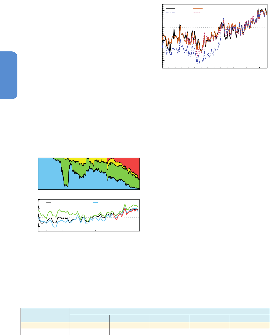
190

Chapter 2 Observations: Atmosphere and Surface

2.4.2 Sea Surface Temperature and Marine Air

Temperature

AR4 concluded that ‘recent’ warming (since the 1950s) is strongly evi-

dent at all latitudes in SST over each ocean. Prominent spatio-temporal

structures including the ENSO and decadal variability patterns in the

Paciﬁc Ocean (Box 2.5) and a hemispheric asymmetry in the Atlantic

Ocean were highlighted as contributors to the regional differences in

surface warming rates, which in turn affect atmospheric circulation.

Since AR4 the availability of metadata has increased, data complete-

ness has improved and a number of new SST products have been pro-

duced. Intercomparisons of data obtained by different measurement

methods, including satellite data, have resulted in better understand-

ing of errors and biases in the record.

2.4.2.1 Advances in Assembling Data Sets and in

Understanding Data Errors

2.4.2.1.1 In situ data records

Historically, most SST observations were obtained from moving ships.

Buoy measurements comprise a signiﬁcant and increasing fraction

of in situ SST measurements from the 1980s onward (Figure 2.15).

Improvements in the understanding of uncertainty have been expe-

dited by the use of metadata (Kent et al., 2007) and the recovery of

1920 1940

0.0

0.2

0.4

0.6

0.8

1.0

Fractional contribution to

global average SST

-0.6

-0.4

-0.2

0.0

0.2

0.4

0.6

0.8

SST anomaly (°C) relative

to 1961-1990

1960 1980 2000

1960 1970 19801950

(a)

(b)

1990 2000

All

ERI/Hull contact sensors

Bucket

Buoy

Figure 2.15 | Temporal changes in the prevalence of different measurement methods

in the International Comprehensive Ocean-Atmosphere Data Set (ICOADS). (a) Fraction-

al contributions of observations made by different measurement methods: bucket obser-

vations (blue), engine room intake (ERI) and hull contact sensor observations (green),

moored and drifting buoys (red), and unknown (yellow). (b) Global annual average sea

surface temperature (SST) anomalies based on different kinds of data: ERI and hull

contact sensor (green), bucket (blue), buoy (red), and all (black). Averages are computed

over all 5° × 5° grid boxes where both ERI/hull and bucket measurements, but not

necessarily buoy data, were available. (Adapted from Kennedy et al., 2011a.)

observer instructions and other related documents. Early data were

systematically cold biased because they were made using canvas or

wooden buckets that, on average, lost heat to the air before the meas-

urements were taken. This effect has long been recognized (Brooks,

1926), and prior to AR4 represented the only artefact adjusted in grid-

ded SST products, such as HadSST2 (Rayner et al., 2006) and ERSST

(Smith et al., 2005, 2008), which were based on ‘bucket correction’

methods by Folland and Parker (1995) and Smith and Reynolds (2002),

respectively. The adjustments, made using ship observations of Night

Marine Air Temperature (NMAT) and other sources, had a striking effect

on the SST global mean estimates: note the difference in 1850–1941

between HadSST2 and International Comprehensive Ocean-Atmos-

phere Data Set (ICOADS) curves in Figure 2.16 (a brief description of

SST and NMAT data sets and their methods is given in Supplementary

Material 2.SM.4.3).

Buckets of improved design and measurement methods with smaller,

on average, biases came into use after 1941 (Figure 2.15, top); aver-

age biases were reduced further in recent decades, but not eliminated

(Figure 2.15, bottom). Increasing density of SST observations made

possible the identiﬁcation (Reynolds et al., 2002, 2010; Kennedy et al.,

2012) and partial correction of more recent period biases (Kennedy et

al., 2011a). In particular, it is hypothesized that the proximity of the

hot engine often biases engine room intake (ERI) measurements warm

(Kent et al., 2010). Because of the prevalence of the ERI measurements

among SST data from ships, the ship SSTs are biased warm by 0.12°C

to 0.18°C on average compared to the buoy data (Reynolds et al., 2010;

Kennedy et al., 2011a, 2012). An assessment of the potential impact

of modern biases can be ascertained by considering the difference

HadSST2

ICOADS

HadSST3

HadNMAT2

1850 1900 1950 2000

Temperature anomaly (ºC)

0.4

0.2

0.0

-0.2

-0.4

-0.6

-0.8

Figure 2.16 | Global annual average sea surface temperature (SST) and Night Marine

Air Temperature (NMAT) relative to a 1961–1990 climatology from gridded data sets

of SST observations (HadSST2 and its successor HadSST3), the raw SST measurement

archive (ICOADS, v2.5) and night marine air temperatures data set HadNMAT2 (Kent et

al., 2013). HadSST2 and HadSST3 both are based on SST observations from versions of

the ICOADS data set, but differ in degree of measurement bias correction.

Data Set

Trends in °C per decade

1880–2012 1901–2012 1901–1950 1951–2012 1979–2012

HadSST3 (Kennedy et al., 2011a) 0.054 ± 0.012 0.067 ± 0.013 0.117 ± 0.028 0.074 ± 0.027 0.124 ± 0.030

HadSST2 (Rayner et al., 2006) 0.051 ± 0.015 0.069 ± 0.012 0.084 ± 0.055 0.098 ± 0.017 0.121 ± 0.033

Table 2.5 | Trend estimates and 90% conﬁdence intervals (Box 2.2) for two subsequent versions of the HadSST data set over ﬁve common periods. HadSST2 has been used in

AR4; HadSST3 is used in this chapter.

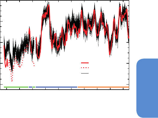
191

Observations: Atmosphere and Surface Chapter 2

between HadSST3 (bias corrections applied throughout) and HadSST2

(bucket corrections only) global means (Figure 2.16): it is particularly

prominent in 1945–1970 period, when rapid changes in prevalence of

ERI and bucket measurements during and after the World War II affect

HadSST2 owing to the uncorrected measurement biases (Thompson et

al., 2008), while these are corrected in HadSST3. Nevertheless, for peri-

ods longer than a century the effect of HadSST3-HadSST2 differences

on linear trend slopes is small relative to the trend uncertainty (Table

2.5). Some degree of independent check on the validity of HadSST3

adjustments comes from a comparison to sub-surface temperature

data (Gouretski et al., 2012) (see Section 3.2).

The traditional approach to modeling random error of in situ SST

data assumed the independence of individual measurements. Kent

and Berry (2008) identiﬁed the need to account for error correlation

for measurements from the same “platform” (i.e., an individual ship

or buoy), while measurement errors from different platforms remain

independent.. Kennedy et al. (2011b) achieved that by introducing

platform-dependent biases, which are constant within the same plat-

form, but change randomly from one platform to another. Accounting

for such correlated errors in HadSST3 resulted in estimated error for

global and hemispheric monthly means that are more than twice the

estimates given by HadSST2. The uncertainty in many, but not all, com-

ponents of the HadSST3 product is represented by the ensemble of its

realizations (Figure 2.17).

Data sets of marine air temperatures (MATs) have traditionally been

restricted to nighttime series only (NMAT data sets) due to the direct

solar heating effect on the daytime measurements, although corrected

daytime MAT records for 1973–present are already available (Berry

and Kent, 2009). Other major biases, affecting both nighttime and day-

time MAT are due to increasing deck height with the general increase

in the size of ships over time and non-standard measurement prac-

tices. Recently these biases were re-examined and explicit uncertainty

calculation undertaken for NMAT by Kent et al. (2013), resulting in the

HadNMAT2 data set.

2.4.2.1.2 Satellite SST data records

Satellite SST data sets are based on measuring electromagnetic radia-

tion that left the ocean surface and got transmitted through the atmos-

phere. Because of the complexity of processes involved, the majority

of such data has to be calibrated on the basis of in situ observations.

The resulting data sets, however, provide a description of global SST

ﬁelds with a level of spatial detail unachievable by in situ data only.

The principal IR sensor is the Advanced Very High Resolution Radiom-

eter (AVHRR). Since AR4, the AVHRR time series has been reprocessed

consistently back to March 1981 (Casey et al., 2010) to create the

AVHRR Pathﬁnder v5.2 data set. Passive microwave data sets of SST

are available since 1997 equatorward of 40° and near-globally since

2002 (Wentz et al., 2000; Gentemann et al., 2004). They are generally

less accurate than IR-based SST data sets, but their superior coverage

in areas of persistent cloudiness provides SST estimates where the IR

record has none (Reynolds et al., 2010).

The (Advanced) Along Track Scanning Radiometer (A)ATSR) series of

three sensors was designed for climate monitoring of SST; their com-

bined record starts in August 1991 and exceeds two decades (it stopped

with the demise of the ENVISAT platform in 2012). The (A)ATSRs are

‘dual-view’ IR radiometers intended to allow atmospheric effects

removal without the use of in situ observations. Since AR4, (A)ATSR

observations have been reprocessed with new estimation techniques

(Embury and Merchant, 2011). The resulting SST products seem to be

more accurate than many in situ observations (Embury et al., 2011). In

terms of monthly global means, the agreement is illustrated in Figure

2.17. By analyzing (A)ATSR and in situ data together, Kennedy at al.

(2012) veriﬁed and extended existing models for biases and random

errors of in situ data.

2.4.2.2 Interpolated SST Products and Trends

SST data sets form a major part of global surface temperature anal-

yses considered in this assessment report. To use an SST data set as

a boundary condition for atmospheric reanalyses products (Box 2.3)

or in atmosphere-only climate simulations (considered in Chapter 9

onwards), gridded data sets with complete coverage over the global

ocean are typically needed. These are usually based on a special form

of kriging (optimal interpolation) procedure that retains large-scale

correlation structures and can accommodate very sparse data cover-

age. For the pre-satellite era (generally, before October 1981) only in

situ data are used; for the latter period some products also use AVHRR

data. Figure 2.18 compares interpolated SST data sets that extend

back to the 19th century with the uninterpolated HadSST3 and Had-

NMAT2 products. Linear trend estimates for global mean SSTs from

those products updated through 2012 are presented in Table 2.6. Dif-

ferences between the trends from different data sets are larger when

the calculation period is shorter (1979–2012) or has lower quality

data (1901–1950); these are due mainly to different data coverage of

underlying observational data sets and bias correction methods used

in these products.

1992 1994 1996 1998 2000 2002 2004 2006 2008 2010

-0.2

0.0

0.2

0.4

0.6

SST anomaly (°C)

ARC D3

ARC D2

HadSST3

ATSR-1 ATSR-2 AATSR

Figure 2.17 | Global monthly mean sea surface temperature (SST) anomalies relative

to a 1961–1990 climatology from satellites (ATSRs) and in situ records (HadSST3). Black

lines: the 100-member HadSST3 ensemble. Red lines: ATSR-based nighttime subsurface

temperature at 0.2 m depth (SST

0.2m

) estimates from the ATSR Reprocessing for Climate

(ARC) project. Retrievals based on three spectral channels (D3, solid line) are more

accurate than retrievals based on only two (D2, dotted line). Contributions of the three

different ATSR missions to the curve shown are indicated at the bottom. The in situ and

satellite records were co-located within 5° × 5° monthly grid boxes: only those where

both data sets had data for the same month were used in the comparison. (Adapted

from Merchant et al. 2012.)

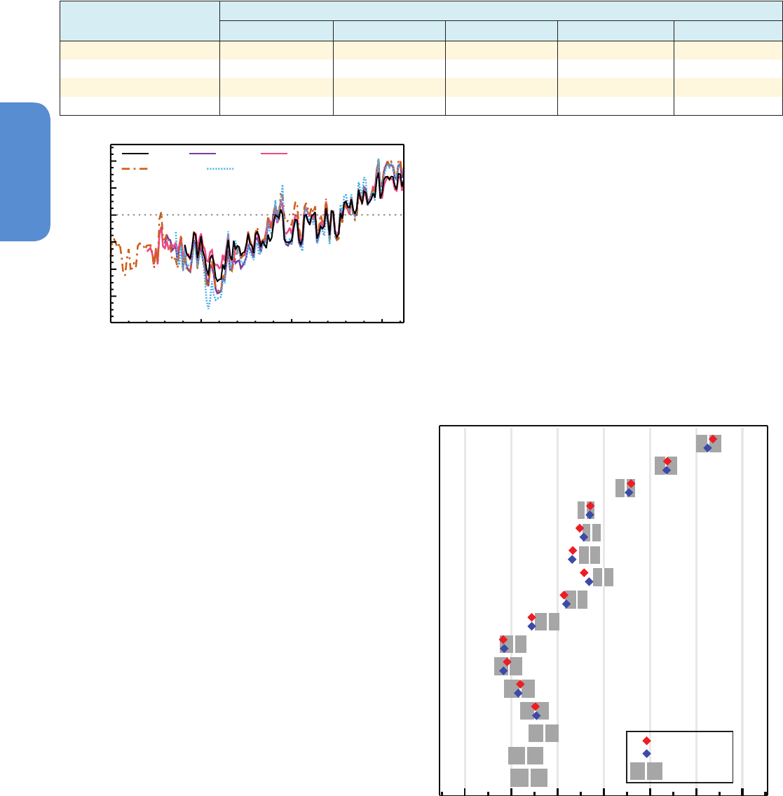
192

Chapter 2 Observations: Atmosphere and Surface

In summary, it is certain that global average sea surface temperatures

(SSTs) have increased since the beginning of the 20th century. Since

AR4, major improvements in availability of metadata and data com-

pleteness have been made, and a number of new global SST records

have been produced. Intercomparisons of new SST data records

obtained by different measurement methods, including satellite data,

have resulted in better understanding of uncertainties and biases in

the records. Although these innovations have helped highlight and

quantify uncertainties and affect our understanding of the character of

changes since the mid-20th century, they do not alter the conclusion

that global SSTs have increased both since the 1950s and since the

late 19th century.

2.4.3 Global Combined Land and Sea Surface

Temperature

AR4 concluded that the GMST had increased, with the last 50 years

increasing at almost double the rate of the last 100 years. Subsequent

developments in LSAT and SST have led to better understanding of the

data and their uncertainties as discussed in preceding sections. This

improved understanding has led to revised global products.

Changes have been made to all three GMST data sets that were used

in AR4 (Hansen et al., 2010; Morice et al., 2012; Vose et al., 2012b).

These are now in somewhat better agreement with each other over

recent years, in large part because HadCRUT4 now better samples the

NH high latitude land regions (Jones et al., 2012; Morice et al., 2012)

which comparisons to reanalyses had shown led to a propensity for

HadCRUT3 to underestimate recent warming (Simmons et al., 2010).

Table 2.6 | Trend estimates and 90% conﬁdence intervals (Box 2.2) for interpolated SST data sets (uninterpolated state-of-the-art HadSST3 data set is included for comparison).

Dash indicates not enough data available for trend calculation.

Data Set

Trends in °C per decade

1880–2012 1901–2012 1901–1950 1951–2012 1979–2012

HadISST (Rayner et al., 2003) 0.042 ± 0.007 0.052 ± 0.007 0.067 ± 0.024 0.064 ± 0.015 0.072 ± 0.024

COBE-SST (Ishii et al., 2005) – 0.058 ± 0.007 0.066 ± 0.032 0.071 ± 0.014 0.073 ± 0.020

ERSSTv3b (Smith et al., 2008) 0.054 ± 0.015 0.071 ± 0.011 0.097 ± 0.050 0.088 ± 0.017 0.105 ± 0.031

HadSST3 (Kennedy et al., 2011a) 0.054 ± 0.012 0.067 ± 0.013 0.117 ± 0.028 0.074 ± 0.027 0.124 ± 0.030

0.4

0.2

0.0

-0.2

-0.4

-0.6

Temperature anomaly (ºC)

1850 1900

1950

2000

COBE HadISST

HadNMAT2

ERSST

HadSST3

Figure 2.18 | Global annual average sea surface temperature (SST) and Night Marine

Air Temperature (NMAT) relative to a 1961–1990 climatology from state of the art data

sets. Spatially interpolated products are shown by solid lines; non-interpolated products

by dashed lines.

Starting in the 1980s each decade has been signiﬁcantly warmer at

the Earth’s surface than any preceding decade since the 1850s in Had-

CRUT4, a data set that explicitly quantiﬁes a large number of sources

of uncertainty (Figure 2.19). Each of the last three decades is also the

warmest in the other two GMST data sets, but these have substan-

tially less mature and complete uncertainty estimates, precluding such

an assessment of signiﬁcance of their decadal differences. The GISS

and MLOST data sets fall outside the 90% CI of HadCRUT4 for several

decades in the 20th century (Figure 2.19). These decadal differences

could reﬂect residual biases in one or more data set, an incomplete

treatment of uncertainties in HadCRUT4.1 or a combination of these

effects (Box 2.1). The data sets utilize different LSAT (Section 2.4.1)

and SST (Section 2.4.2) component records (Supplementary Material

2.SM.4.3.4) that in the case of SST differ somewhat in their multi-dec-

adal trend behaviour (Table 2.6 compare HadSST3 and ERSSTv3b).

-0.6 -0.4 -0.2 0.0 0.2 0.4 0.6

Temperature difference from 1961-1990 (

1850s

1860s

1870s

1880s

1890s

1900s

1910s

1920s

1930s

1940s

1950s

1960s

1970s

1980s

1990s

2000s

MLOST

GISS

HadCRUT4

Figure 2.19 | Decadal global mean surface temperature (GMST) anomalies (white

vertical lines in grey blocks) and their uncertainties (90% conﬁdence intervals as grey

blocks) based upon the land-surface air temperature (LSAT) and sea surface tempera-

ture (SST) combined HadCRUT4 (v4.1.1.0) ensemble (Morice et al., 2012). Anomalies

are relative to a 1961–1990 climatology. 1850s indicates the period 1850-1859, and

so on. NCDC MLOST and GISS data set best-estimates are also shown.

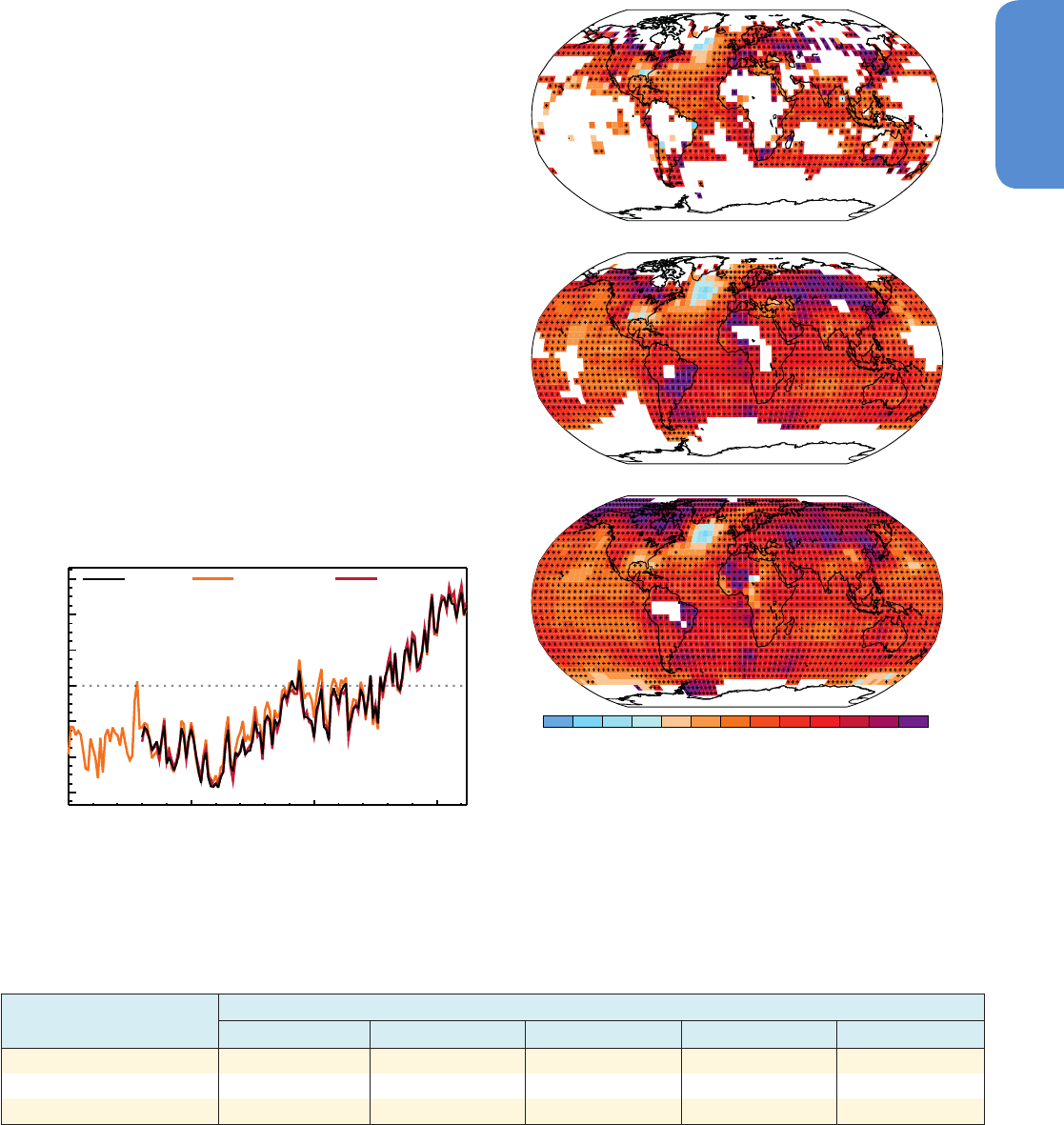
193

Observations: Atmosphere and Surface Chapter 2

All ten of the warmest years have occurred since 1997, with 2010 and

2005 effectively tied for the warmest year on record in all three prod-

ucts. However, uncertainties on individual annual values are sufﬁcient-

ly large that the ten warmest years are statistically indistinguishable

from one another. The global-mean trends are signiﬁcant for all data

sets and multi-decadal periods considered in Table 2.7. Using Had-

CRUT4 and its uncertainty estimates, the warming from 1850–1900 to

1986–2005 (reference period for the modelling chapters and Annex I)

is 0.61 [0.55 to 0.67] °C (90% conﬁdence interval), and the warming

from 1850–1900 to 2003–2012 (the most recent decade) is 0.78 [0.72

to 0.85] °C (Supplementary Material 2.SM.4.3.3).

Differences between data sets are much smaller than both interannual

variability and the long-term trend (Figure 2.20). Since 1901 almost the

whole globe has experienced surface warming (Figure 2.21). Warming

has not been linear; most warming occurred in two periods: around

1900 to around 1940 and around 1970 onwards (Figure 2.22. Shorter

periods are noisier and so proportionately less of the sampled globe

exhibits statistically signiﬁcant trends at the grid box level (Figure

2.22). The two periods of global mean warming exhibit very distinct

spatial signatures. The early 20th century warming was largely a NH

mid- to high-latitude phenomenon, whereas the more recent warm-

ing is more global in nature. These distinctions may yield important

information as to causes (Chapter 10). Differences between data sets

are larger in earlier periods (Figures 2.19, 2.20), particularly prior to

the 1950s when observational sampling is much more geographically

incomplete (and many of the well sampled areas may have been glob-

ally unrepresentative (Brönnimann, 2009)), data errors and subsequent

methodological impacts are larger (Thompson et al., 2008), and differ-

ent ways of accounting for data void regions are more important (Vose

et al., 2005b).

Table 2.7 | Same as Table 2.4, but for global mean surface temperature (GMST) over ﬁve common periods.

Data Set

Trends in °C per decade

1880–2012 1901–2012 1901–1950 1951–2012 1979–2012

HadCRUT4 (Morice et al., 2012) 0.062 ± 0.012 0.075 ± 0.013 0.107 ± 0.026 0.106 ± 0.027 0.155 ± 0.033

NCDC MLOST (Vose et al., 2012b) 0.064 ± 0.015 0.081 ± 0.013 0.097 ± 0.040 0.118 ± 0.021 0.151 ± 0.037

GISS (Hansen et al., 2010) 0.065 ± 0.015 0.083 ± 0.013 0.090 ± 0.034 0.124 ± 0.020 0.161 ± 0.033

1850 1900

1950

2000

Temperature anomaly (ºC)

GISSHadCRUT4MLOST

0.6

0.4

0.2

0.0

-0.2

-0.4

-0.6

Trend (ºC over period)

-0.6 -0.4 -0.2 00.2 0.40.6 0.81.1.251.5 1.75 2.5

HadCRUT4 1901-2012

MLOST 1901-2012

GISS 1901-2012

Figure 2.20 | Annual global mean surface temperature (GMST) anomalies relative to a

1961–1990 climatology from the latest version of the three combined land-surface air

temperature (LSAT) and sea surface temperature (SST) data sets (HadCRUT4, GISS and

NCDC MLOST). Published data set uncertainties are not included for reasons discussed

in Box 2.1.

Figure 2.21 | Trends in surface temperature from the three data sets of Figure 2.20

for 1901–2012. White areas indicate incomplete or missing data. Trends have been

calculated only for those grid boxes with greater than 70% complete records and more

than 20% data availability in ﬁrst and last decile of the period. Black plus signs (+)

indicate grid boxes where trends are signiﬁcant (i.e., a trend of zero lies outside the 90%

conﬁdence interval). Differences in coverage primarily reﬂect the degree of interpolation

to account for data void regions undertaken by the data set providers ranging from none

beyond grid box averaging (HadCRUT4) to substantial (GISS).

Much interest has focussed on the period since 1998 and an observed

reduction in warming trend, most marked in NH winter (Cohen et al.,

2012). Various investigators have pointed out the limitations of such

short-term trend analysis in the presence of auto-correlated series var-

iability and that several other similar length phases of no warming

exist in all the observational records and in climate model simulations

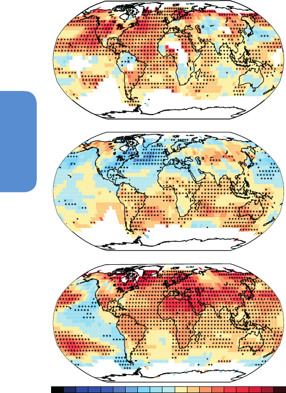
194

Chapter 2 Observations: Atmosphere and Surface

MLOST 1911-1940

MLOST 1951-1980

MLOST 1981-2012

Trend (°C per decade)

-1.25 -1

-0.8 -0.6

-0.5

-0.4

-0.3

-0.2

-0.1 0 0.1 0.2

0.3

0.4 0.5

0.6

0.8 1 1.25

Figure 2.22 | Trends in surface temperature from NCDC MLOST for three non-

consectutive shorter periods (1911–1940; 1951–1980; 1981–2012). White areas

indicate incomplete or missing data. Trends and signiﬁcance have been calculated as

in Figure 2.21.

(Easterling and Wehner, 2009; Peterson et al., 2009; Liebmann et al.,

2010; Foster and Rahmstorf, 2011; Santer et al., 2011). This issue is

discussed in the context of model behaviour, forcings and natural var-

iability in Box 9.2 and Section 10.3.1. Regardless, all global combined

LSAT and SST data sets exhibit a statistically non-signiﬁcant warming

trend over 1998–2012 (0.042°C ± 0.093°C per decade (HadCRUT4);

0.037°C ± 0.085°C per decade (NCDC MLOST); 0.069°C ± 0.082°C per

decade (GISS)). An average of the trends from these three data sets

yields an estimated change for the 1998–2012 period of 0.05 [–0.05 to

+0.15] °C per decade. Trends of this short length are very sensitive to

the precise period selection with trends calculated in the same manner

for the 15-year periods starting in 1995, 1996, and 1997 being 0.13

[0.02 to 0.24], 0.14 [0.03 to 0.24] and 0.07 [–0.02 to 0.18] (all °C per

decade), respectively.

In summary, it is certain that globally averaged near surface temper-

atures have increased since the late 19th century. Each of the past

three decades has been warmer than all the previous decades in

the instrumental record, and the decade of the 2000s has been the

warmest. The globally averaged combined land and ocean surface

temperature data as calculated by a linear trend, show a warming

of 0.85 [0.65 to 1.06] °C, over the period 1880–2012, when multiple

independently produced datasets exist, about 0.89°C [0.69 to 1.08] °C

over the period 1901–2012, and about 0.72 [0.49° to 0.89] °C over

the period 1951–2012. The total increase between the average of the

1850–1900 period and the 2003–2012 period is 0.78 [0.72 to 0.85] °C

and the total increase between the average of the 1850–1900 period

and the reference period for projections 1986−2005 is 0.61 [0.55 to

0.67] °C, based on the single longest dataset available. For the lon-

gest period when calculation of regional trends is sufﬁciently complete

(1901–2012), almost the entire globe has experienced surface warm-

ing. In addition to robust multi-decadal warming, global mean surface

temperature exhibits substantial decadal and interannual variability.

Owing to natural variability, trends based on short records are very

sensitive to the beginning and end dates and do not in general reﬂect

long-term climate trends. As one example, the rate of warming over

the past 15 years (1998–2012; 0.05 [–0.05 to +0.15] °C per decade),

which begins with a strong El Niño, is smaller than the rate calculated

since 1951 (1951–2012; 0.12 [0.08 to 0.14] °C per decade)Trends for

15-year periods starting in 1995, 1996, and 1997 are 0.13 [0.02 to

0.24], 0.14 [0.03 to 0.24] and 0.07 [–0.02 to 0.18], respectively..

2.4.4 Upper Air Temperature

AR4 summarized that globally the troposphere had warmed at a rate

greater than the GMST over the radiosonde record, while over the

shorter satellite era the GMST and tropospheric warming rates were

indistinguishable. Trends in the tropics were more uncertain than

global trends although even this region was concluded to be warming.

Globally, the stratosphere was reported to be cooling over the satellite

era starting in 1979. New advances since AR4 have highlighted the

substantial degree of uncertainty in both satellite and balloon-borne

radiosonde records and led to some revisions and improvements in

existing products and the creation of a number of new data products.

2.4.4.1 Advances in Multi-Decadal Observational Records

The major global radiosonde records extend back to 1958, with tem-

peratures, measured as the balloon ascends, reported at mandatory

pressure levels. Satellites have monitored tropospheric and lower strat-

ospheric temperature trends since late 1978 through the Microwave

Sounding Unit (MSU) and its follow-on Advanced Microwave Sound-

ing Unit (AMSU) since 1998. These measures of upwelling radiation

represent bulk (volume averaged) atmospheric temperature (Figure

2.23). The ‘Mid-Tropospheric’ (MT) MSU channel that most directly cor-

responds to the troposphere has 10 to 15% of its signal from both the

skin temperature of the Earth’s surface and the stratosphere. Two alter-

native approaches have been suggested for removing the stratospheric

component based on differencing of view angles (LT) and statistical

recombination (*G) with the ‘Lower Stratosphere’ (LS) channel (Spen-

cer and Christy, 1992; Fu et al., 2004). The MSU satellite series also

included a Stratospheric Sounding Unit (SSU) that measured at higher

altitudes (Seidel et al., 2011).

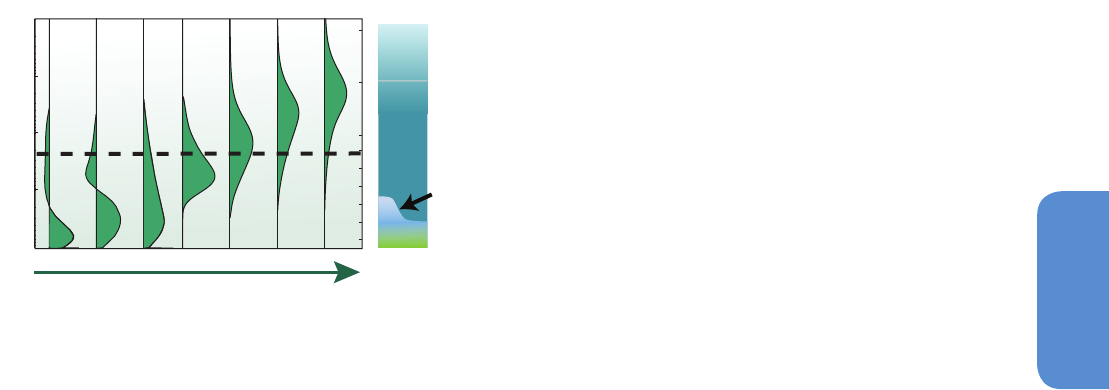
195

Observations: Atmosphere and Surface Chapter 2

At the time of AR4 there were only two ‘global’ radiosonde data sets

that included treatment of homogeneity issues: RATPAC (Free et al.,

2005) and HadAT (Thorne et al., 2005). Three additional estimates

have appeared since AR4 based on novel and distinct approaches.

A group at the University of Vienna have produced RAOBCORE and

RICH (Haimberger, 2007; Haimberger et al., 2008, 2012) using ERA

reanalysis products (Box 2.3). Sherwood and colleagues developed an

iterative universal kriging approach for radiosonde data to create IUK

(Sherwood et al., 2008) and concluded that non-climatic data issues

leading to spurious cooling remained in the deep tropics even after

homogenization. The HadAT group created an automated version,

undertook systematic experimentation and concluded that the para-

metric uncertainty (Box 2.1) was of the same order of magnitude as

the apparent climate signal (McCarthy et al., 2008; Titchner et al.,

2009; Thorne et al., 2011). A similar ensemble approach has also been

applied to the RICH product (Haimberger et al., 2012). These various

ensembles and new products exhibit more tropospheric warming / less

stratospheric cooling than pre-existing products at all levels. Globally

the radiosonde records all imply the troposphere has warmed and the

stratosphere cooled since 1958 but with uncertainty that grows with

height and is much greater outside the better-sampled NH extra-trop-

ics (Thorne et al., 2011; Haimberger et al., 2012), where it is of the

order 0.1°C per decade.

For MSU, AR4 considered estimates produced from three groups: UAH

(University of Alabama in Huntsville); RSS (Remote Sensing Systems)

and VG2 (now no longer updated). A new product has been creat-

ed by NOAA labelled STAR, using a fundamentally distinct approach

for the critical inter-satellite warm target calibration step (Zou et al.,

2006a). STAR exhibits more warming/less cooling at all levels than

UAH and RSS. For MT and LS, Zou and Wang (2010) concluded that

this does not relate primarily to use of their inter-satellite calibration

technique but rather differences in other processing steps. RSS also

produced a parametric uncertainty ensemble (Box 2.1) employing a

Monte Carlo approach allowing methodological inter-dependencies to

be fully expressed (Mears et al., 2011). For large-scale trends dominant

effects were inter-satellite offset determinations and, for tropospheric

channels, diurnal drift. Uncertainties were concluded to be of the order

0.1°C per decade at the global mean for both tropospheric channels

(where it is of comparable magnitude to the long-term trends) and the

stratospheric channel.

SSU provides the only long-term near-global temperature data above

the lower stratosphere, with the series terminating in 2006. Some

AMSU-A channels have replaced this capability and efforts to under-

stand the effect of changed measurement properties have been under-

taken (Kobayashi et al., 2009). Until recently only one SSU data set

existed (Nash and Edge, 1989), updated by Randel et al. (2009). Liu and

Weng (2009) have produced an intermediate analysis for Channels 25

and 26 (but not Channel 27). Wang et al. (2012g), building on insights

from several of these recent studies, have produced a more complete

analysis. Differences between the independent estimates are much

larger than differences between MSU records or radiosonde records

at lower levels, with substantial inter-decadal time series behaviour

departures, zonal trend structure, and global trend differences of the

order 0.5°C per decade (Seidel et al., 2011; Thompson et al., 2012;

Wang et al., 2012g). Although all SSU data sets agree that the strato-

sphere is cooling, there is therefore low conﬁdence in the details above

the lower stratosphere.

In summary, many new data sets have been produced since AR4 from

radiosondes and satellites with renewed interest in satellite measure-

ments above the lower stratosphere. Several studies have attempted

to quantify the parametric uncertainty (Box 2.1) more rigorously. These

various data sets and analyses have served to highlight the degree of

uncertainty in the data and derived products.

2.4.4.2 Intercomparisons of Various Long-Term Radiosonde

and MSU Products

Since AR4 there have been a large number of intercomparisons between

radiosonde and MSU data sets. Interpretation is complicated, as most

studies considered data set versions that have since been superseded.

Several studies compared UAH and RSS products to local, regional or

global raw/homogenized radiosonde data (Christy and Norris, 2006,

2009; Christy et al., 2007, 2010, 2011; Randall and Herman, 2008;

Mears et al., 2012; Po-Chedley and Fu, 2012). Early studies focussed on

the time of transition from NOAA-11 to NOAA-12 (early 1990s) which

indicated an apparent issue in RSS. Christy et al. (2007) noted that this

coincided with the Mt Pinatubo eruption and that RSS was the only

product, either surface or tropospheric, that exhibited tropical warm-

ing immediately after the eruption when cooling would be expected.

Using reanalysis data Bengtsson and Hodges (2011) also found evi-

dence of a potential jump in RSS in 1993 over the tropical oceans.

Mears et al. (2012) cautioned that an El Niño event quasi-simultane-

ous with Pinatubo complicates interpretation. They also highlighted

several other periods of disagreement between radiosonde records

and MSU records. All MSU records were most uncertain when satellite

orbits are drifting rapidly (Christy and Norris, 2006, 2009). Mears et

al. (2011) found that trend differences between RSS and other data

sets could not be explained in many cases by parametric uncertainties

in RSS alone. It was repeatedly cautioned that there were potential

common biases (of varying magnitude) between the different MSU

Pressure (hPa)

Height (km)

Weight

0.1

1.0

100

1000

MT LS SSU 25 SSU 26 SSU 27

Tropopause

Level

Poles

Stratosphere

Troposphere

Mesosphere

opics

Surface

Figure 2.23 | Vertical weighting functions for those satellite temperature retrievals

discussed in this chapter (modiﬁed from Seidel et al. (2011)). The dashed line indicates

the typical maximum altitude achieved in the historical radiosonde record. The three SSU

channels are denoted by the designated names 25, 26 and 27. LS (Lower Stratosphere)

and MT (Mid Troposphere) are two direct MSU measures and LT (Lower Troposphere)

and *G (Global Troposphere) are derived quantities from one or more of these that

attempt to remove the stratospheric component from MT.

196

Chapter 2 Observations: Atmosphere and Surface

records or between the different radiosonde records which complicate

intercomparisons (Christy and Norris, 2006, 2009; Mears et al., 2012).

In summary, assessment of the large body of studies comparing var-

ious long-term radiosonde and MSU products since AR4 is hampered

by data set version changes, and inherent data uncertainties. These

factors substantially limit the ability to draw robust and consistent

inferences from such studies about the true long-term trends or the

value of different data products.

2.4.4.3 Additional Evidence from Other Technologies

and Approaches

Global Positioning System (GPS) radio occultation (RO) currently repre-

sents the only self-calibrated SI traceable raw satellite measurements

(Anthes et al., 2008; Anthes, 2011). The fundamental observation is

time delay of the occulted signal’s phase traversing the atmosphere.

The time delay is a function of several atmospheric physical state vari-

ables. Subsequent analysis converts the time delay to temperature and

other parameters, which inevitably adds some degree of uncertainty to

the derived temperature data. Intercomparisons of GPS-RO products

show that differences are largest for derived geophysical parameters

(including temperature), but are still small relative to other observing

technologies (Ho et al., 2012). Comparisons to MSU and radiosondes

(Kuo et al., 2005; Ho et al., 2007, 2009a, 2009b; He et al., 2009; Bar-

inger et al., 2010; Sun et al., 2010; Ladstadter et al., 2011) show sub-

stantive agreement in interannual behaviour, but also some multi-year

drifts that require further examination before this additional data

source can usefully arbitrate between different MSU and radiosonde

trend estimates.

Atmospheric winds are driven by thermal gradients. Radiosonde winds

are far less affected by time-varying biases than their temperatures

(Gruber and Haimberger, 2008; Sherwood et al., 2008; Section 2.7.3).

Allen and Sherwood (2007) initially used radiosonde wind to infer

temperatures within the Tropical West Paciﬁc warm pool region, then

extended this to a global analysis (Allen and Sherwood, 2008) yielding

a distinct tropical upper tropospheric warming trend maximum within

the vertical proﬁle, but with large uncertainty. Winds can only quan-

tify relative changes and require an initialization (location and trend

at that location) (Allen and Sherwood, 2008). The large uncertainty

range was predominantly driven by this initialization choice, a ﬁnding

later conﬁrmed by Christy et al. (2010), who in addition questioned

the stability given the sparse geographical sampling, particularly in the

tropics, and possible systematic sampling effects amongst other poten-

tial issues. Initializing closer to the tropics tended to reduce or remove

the appearance of a tropical upper tropospheric warming trend maxi-

mum (Allen and Sherwood, 2008; Christy et al., 2010). There is only low

conﬁdence in trends inferred from ‘thermal winds’ given the relative

immaturity of the analyses and their large uncertainties.

In summary, new technologies and approaches have emerged since

AR4. However, these new technologies and approaches either consti-

tute too short a record or are too immature to inform assessments of

long-term trends at the present time.

2.4.4.4 Synthesis of Free Atmosphere Temperature Estimates

Global-mean lower tropospheric temperatures have increased since the

mid-20th century (Figure 2.24, bottom). Structural uncertainties (Box

2.1) are larger than at the surface but it can still be concluded that glob-

ally the troposphere has warmed (Table 2.8). On top of this long-term

trend are superimposed short-term variations that are highly correlated

with those at the surface but of somewhat greater amplitude. Global

mean lower stratospheric temperatures have decreased since the mid-

20th century punctuated by short-lived warming events associated with

explosive volcanic activity (Figure 2.24a). However, since the mid-1990s

little net change has occurred. Cooling rates are on average greater

from radiosonde data sets than MSU data sets. This very likely relates

to widely recognized cooling biases in radiosondes (Mears et al., 2006)

which all data set producers explicitly caution are likely to remain to

some extent in their ﬁnal products (Free and Seidel, 2007; Haimberger

et al., 2008; Sherwood et al., 2008; Thorne et al., 2011).

In comparison to the surface (Figure 2.22), tropospheric layers exhibit

smoother geographic trends (Figure 2.25) with warming dominating

cooling north of approximately 45°S and greatest warming in high

northern latitudes. The lower stratosphere cooled almost everywhere

but this cooling exhibits substantial large-scale structure. Cooling is

greatest in the highest southern latitudes and smallest in high northern

latitudes. There are also secondary stratospheric cooling maxima in the

mid-latitude regions of each hemisphere.

Available global and regional trends from radiosondes since 1958

(Figure 2.26) show agreement that the troposphere has warmed and

the stratosphere cooled. While there is little ambiguity in the sign of the

changes, the rate and vertical structure of change are distinctly data

set dependent, particularly in the stratosphere. Differences are greatest

in the tropics and SH extra-tropics where the historical radiosonde data

coverage is poorest. Not shown in the ﬁgure for clarity are estimates

of parametric data set uncertainties or trend-ﬁt

uncertainties—both of

which are of the order of at least 0.1°C per decade (Section 2.4.4.1).

Differences in trends between available radiosonde data sets are

greater during the satellite era than for the full radiosonde period of

record in all regions and at most levels (Figure 2.27; cf. Figure 2.26). The

RAOBCORE product exhibits greater vertical trend gradients than other

data sets and it has been posited that this relates to its dependency

on reanalysis ﬁelds (Sakamoto and Christy, 2009; Christy et al., 2010).

MSU trend estimates in the troposphere are generally bracketed by the

radiosonde range. In the stratosphere MSU deep layer estimates tend

to show slightly less cooling. Over both 1958–2011 and 1979–2011

there is some evidence in the radiosonde products taken as a whole

that the tropical tropospheric trends increase with height. But the mag-

nitude and the structure is highly data set dependent.

In summary, based on multiple independent analyses of measurements

from radiosondes and satellite sensors it is virtually certain that global-

ly the troposphere has warmed and the stratosphere has cooled since

the mid-20th century. Despite unanimous agreement on the sign of the

trends, substantial disagreement exists among available estimates as

to the rate of temperature changes, particularly outside the NH extra-

tropical troposphere, which has been well sampled by radiosondes.

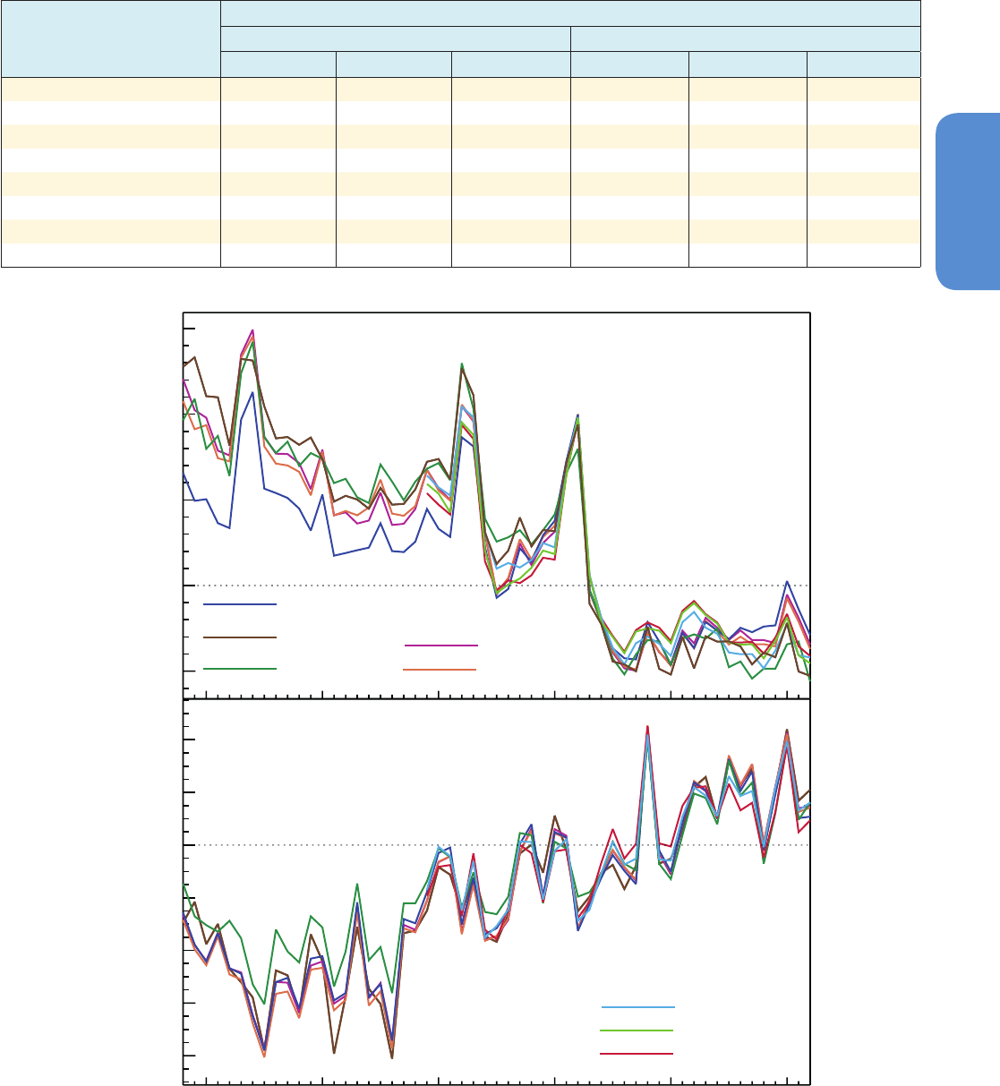
197

Observations: Atmosphere and Surface Chapter 2

Figure 2.24 | Global annual average lower stratospheric (top) and lower tropospheric (bottom) temperature anomalies relative to a 1981–2010 climatology from different data

sets. STAR does not produce a lower tropospheric temperature product. Note that the y-axis resolution differs between the two panels.

1.5

1.0

0.5

0.0

-0.5

(a)

(b)

Temperature anomaly (ºC)

1960 1970 1980 1990 2000 2010

Lower stratosphere

Lower troposphere

Temperature anomaly (ºC)

0.4

0.2

0.0

-0.2

-0.4

-0.6

-0.8

HadAT2

RAOBCORE 1.5

UAH

RICH - obs

RATPACB

STAR

RICH - tau

RSS

Table 2.8 | Trend estimates and 90% conﬁdence intervals (Box 2.2) for radiosonde and MSU data set global average values over the radiosonde (1958–2012) and satellite periods

(1979–2012). LT indicates Lower Troposphere, MT indicates Mid Troposphere and LS indicates Lower Stratosphere (Figure 2.23. Satellite records start only in 1979 and STAR do

not produce an LT product.

Data Set

Trends in °C per decade

1958–2012 1979–2012

LT MT LS LT MT LS

HadAT2 (Thorne et al., 2005) 0.159 ± 0.038 0.095 ± 0.034 –0.339 ± 0.086 0.162 ± 0.047 0.079 ± 0.057 –0.436 ± 0.204

RAOBCORE 1.5 (Haimberger et al., 2012) 0.156 ± 0.031 0.109 ± 0.029 –0.186 ± 0.087 0.139 ± 0.049 0.079 ± 0.054 –0.266 ± 0.227

RICH-obs (Haimberger et al., 2012) 0.162 ± 0.031 0.102 ± 0.029 –0.285 ± 0.087 0.158 ± 0.046 0.081 ± 0.052 –0.331 ± 0.241

RICH-tau (Haimberger et al., 2012) 0.168 ± 0.032 0.111 ± 0.030 –0.280 ± 0.085 0.160 ± 0.046 0.083 ± 0.052 –0.345 ± 0.238

RATPAC (Free et al., 2005) 0.136 ± 0.028 0.076 ± 0.028 –0.338 ± 0.092 0.128 ± 0.044 0.039 ± 0.051 –0.468 ± 0.225

UAH (Christy et al., 2003) 0.138 ± 0.043 0.043 ± 0.042 –0.372 ± 0.201

RSS (Mears and Wentz, 2009a, 2009b) 0.131 ± 0.045 0.079 ± 0.043 –0.268 ± 0.177

STAR (Zou and Wang, 2011) 0.123 ± 0.047 –0.320 ± 0.175

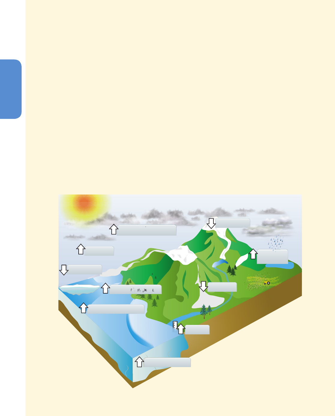
198

Chapter 2 Observations: Atmosphere and Surface

Frequently Asked Questions

FAQ 2.1 | How Do We Know the World Has Warmed?

Evidence for a warming world comes from multiple independent climate indicators, from high up in the atmosphere

to the depths of the oceans. They include changes in surface, atmospheric and oceanic temperatures; glaciers; snow

cover; sea ice; sea level and atmospheric water vapour. Scientists from all over the world have independently veri-

ﬁed this evidence many times. That the world has warmed since the 19th century is unequivocal.

Discussion about climate warming often centres on potential residual biases in temperature records from land-

based weather stations. These records are very important, but they only represent one indicator of changes in the

climate system. Broader evidence for a warming world comes from a wide range of independent physically consis-

tent measurements of many other, strongly interlinked, elements of the climate system (FAQ 2.1, Figure 1).

A rise in global average surface temperatures is the best-known indicator of climate change. Although each year and

even decade is not always warmer than the last, global surface temperatures have warmed substantially since 1900.

Warming land temperatures correspond closely with the observed warming trend over the oceans. Warming oce-

anic air temperatures, measured from aboard ships, and temperatures of the sea surface itself also coincide, as

borne out by many independent analyses.

The atmosphere and ocean are both ﬂuid bodies, so warming at the surface should also be seen in the lower atmo-

sphere, and deeper down into the upper oceans, and observations conﬁrm that this is indeed the case. Analyses of

measurements made by weather balloon radiosondes and satellites consistently show warming of the troposphere,

the active weather layer of the atmosphere. More than 90% of the excess energy absorbed by the climate system

since at least the 1970s has been stored in the oceans as can be seen from global records of ocean heat content

going back to the 1950s. (continued on next page)

FAQ 2.1, Figure 1 | Independent analyses of many components of the climate system that would be expected to change in a warming world exhibit trends

consistent with warming (arrow direction denotes the sign of the change), as shown in FAQ 2.1, Figure 2.

Temperature

Over Land

Ocean Heat Content

Water Vapor

Air Temperature

in the lowest few Km (troposphere)

Marine Air Temperature

Snow Cover

Sea Level

Glacier Volume

Sea Surface Temperature

Sea Ice Area

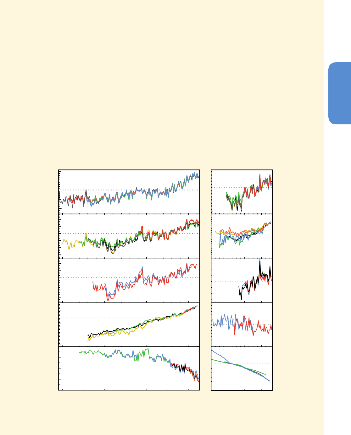
199

Observations: Atmosphere and Surface Chapter 2

As the oceans warm, the water itself expands. This expansion is one of the main drivers of the independently

observed rise in sea levels over the past century. Melting of glaciers and ice sheets also contribute, as do changes in

storage and usage of water on land.

A warmer world is also a moister one, because warmer air can hold more water vapour. Global analyses show that

speciﬁc humidity, which measures the amount of water vapour in the atmosphere, has increased over both the land

and the oceans.

The frozen parts of the planet—known collectively as the cryosphere—affect, and are affected by, local changes

in temperature. The amount of ice contained in glaciers globally has been declining every year for more than 20

years, and the lost mass contributes, in part, to the observed rise in sea level. Snow cover is sensitive to changes in

temperature, particularly during the spring, when snow starts to melt. Spring snow cover has shrunk across the NH

since the 1950s. Substantial losses in Arctic sea ice have been observed since satellite records began, particularly at

the time of the mimimum extent, which occurs in September at the end of the annual melt season. By contrast, the

increase in Antarctic sea ice has been smaller.

Individually, any single analysis might be unconvincing, but analysis of these different indicators and independent

data sets has led many independent research groups to all reach the same conclusion. From the deep oceans to the

top of the troposphere, the evidence of warmer air and oceans, of melting ice and rising seas all points unequivo-

cally to one thing: the world has warmed since the late 19th century (FAQ 2.1, Figure 2).

FAQ 2.1, Figure 2 | Multiple independent indicators of a changing global climate. Each line represents an independently derived estimate of change in the climate

element. In each panel all data sets have been normalized to a common period of record. A full detailing of which source data sets go into which panel is given in the

Supplementary Material 2.SM.5.

FAQ 2.1 (continued)

Land surface air temperature: 4 datasets

Mass balance (10

GT)

1.0

0.5

0.0

-0.5

-1.0

0.4

0.2

0.0

-0.2

-0.4

-0.6

0.4

0.2

0.0

-0.2

-0.4

-0.6

-5

-10

-15

0.4

0.2

0.0

-0.2

-10

0.6

0.4

0.2

0.0

-0.2

-0.4

-0.6

-0.8

100

-50

-100

-150

-200

Tropospheric temperature:

7 datasets

Ocean heat content(0-700m):

5 datasets

Specific humidity:

4 datasets

Glacier mass balance:

3 datasets

Sea-surface temperature: 5 datasets

Marine air temperature: 2 datasets

Sea level: 6 datasets

1850 1900 1950 2000

1940 1960 1980 2000

Summer arctic sea-ice extent: 6 datasets

Sea level

anomaly (mm)

Temperature

anomaly (ºC)

Temperature

anomaly (ºC)

Temperature

anomaly (ºC)

Temperature

anomaly (ºC)

Ocean heat content

anomaly (10

Specific humidity

anomaly (g/kg)

Extent anomaly (10

)

-2

-4

-6

Extent (10

)

Year Year

Northern hemisphere (March-

April) snow cover: 2 datasets

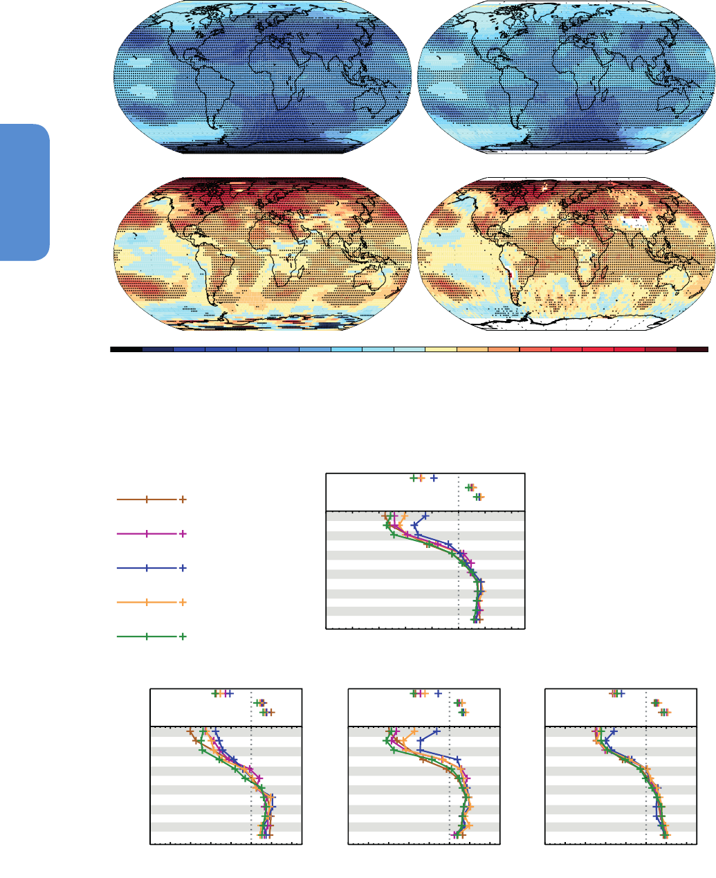
200

Chapter 2 Observations: Atmosphere and Surface

UAH LS

UAH LT RSS LT

RSS LS

Trend (°C per decade)

-1.25-1.0-0.8-0.6-0.5-0.4-0.3-0.2-0.10 0.20.3 0.40.60.50.8 1.01.250.1

Figure 2.25 | Trends in MSU upper air temperature over 1979–2012 from UAH (left-hand panels) and RSS (right-hand panels) and for LS (top row) and LT (bottom row). Data

are temporally complete within the sampled domains for each data set. White areas indicate incomplete or missing data. Black plus signs (+) indicate grid boxes where trends are

signiﬁcant (i.e., a trend of zero lies outside the 90% conﬁdence interval).

Radiosonde Datasets

HadAT2

RICH-obs

RAOBCORE1.5

RICH-tau

RATPACB

Global

SH Extra-Tropics NH Extra-TropicsTropics

Trend (ºC per decade) Trend (ºC per decade)

Trend (ºC per decade)

-1.0 -0.8 -0.6 -0.4 -0.2 0.00.2 0.4-1.0-0.8-0.6-0.4-0.20.0 0.20.4 -1.0 -0.8 -0.6 -0.4 -0.2 0.0 0.2 0.4

-1.0 -0.8 -0.6 -0.4 -0.2 0.00.2 0.4

100

150

200

250

300

400

500

700

850

100

150

200

250

300

400

500

700

850

100

150

200

250

300

400

500

700

850

Pressure (hPa)

100

150

200

250

300

400

500

700

850

Figure 2.26 | Trends in upper air temperature for all available radiosonde data products that contain records for 1958–2012 for the globe (top) and tropics (20°N to 20°S) and

extra-tropics (bottom). The bottom panel trace in each case is for trends on distinct pressure levels. Note that the pressure axis is not linear. The top panel points show MSU layer

equivalent measure trends. MSU layer equivalents have been processed using the method of Thorne et al. (2005). No attempts have been made to sub-sample to a common data

mask.

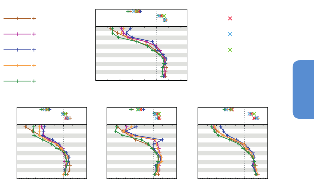
201

Observations: Atmosphere and Surface Chapter 2

Radiosonde Datasets

HadAT2

RICH-obs

RAOBCORE1.5

RICH-tau

RATPACB

Satellite Datasets

RSS

UAH

STAR

Global

SH Extra-Tropics NH Extra-TropicsTropics

Trend (ºC per decade) Trend (ºC per decade)

Trend (ºC per decade)

-1.0 -0.8 -0.6 -0.4 -0.2 0.00.2 0.4-1.0-0.8-0.6-0.4-0.20.0 0.2 0.4 -1.0 -0.8 -0.6 -0.4 -0.2 0.0 0.20.4

-1.0 -0.8 -0.6 -0.4 -0.2 0.00.2 0.4

100

150

200

250

300

400

500

700

850

100

150

200

250

300

400

500

700

850

100

150

200

250

300

400

500

700

850

Pressure (hPa)

100

150

200

250

300

400

500

700

850

Figure 2.27 | As Figure 2.26 except for the satellite era 1979–2012 period and including MSU products (RSS, STAR and UAH).

Hence there is only medium conﬁdence in the rate of change and its

vertical structure in the NH extratropical troposphere and low conﬁ-

dence elsewhere.

2.5 Changes in Hydrological Cycle

This section covers the main aspects of the hydrological cycle, including

large-scale average precipitation, stream ﬂow and runoff, soil mois-

ture, atmospheric water vapour, and clouds. Meteorological drought is

assessed in Section 2.6. Ocean precipitation changes are assessed in

Section 3.4.3 and changes in the area covered by snow in Section 4.5.

2.5.1 Large-Scale Changes in Precipitation

2.5.1.1 Global Land Areas

AR4 concluded that precipitation has generally increased over land

north of 30°N over the period 1900–2005 but downward trends dom-

inate the tropics since the 1970s. AR4 included analysis of both the

GHCN (Vose et al., 1992) and CRU (Mitchell and Jones, 2005) gauge-

based precipitation data sets for the globally averaged annual pre-

cipitation over land. For both data sets the overall linear trend from

1900 to 2005 (1901–2002 for CRU) was positive but not statistically

signiﬁcant (Table 3.4 from AR4). Other periods covered in AR4 (1951–

2005 and 1979–2005) showed a mix of negative and positive trends

depending on the data set.

Since AR4, existing data sets have been updated and a new data set

developed. Figure 2.28 shows the century-scale variations and trends

on globally and zonally averaged annual precipitation using ﬁve data

sets: GHCN V2 (updated through 2011; Vose et al., 1992), Global Pre-

cipitation Climatology Project V2.2 (GPCP) combined raingauge–satel-

lite product (Adler et al., 2003), CRU TS 3.10.01 (updated from Mitchell

and Jones, 2005), Global Precipitation Climatology Centre V6 (GPCC)

data set (Becker et al., 2013) and a reconstructed data set by Smith et

al. (2012). Each data product incorporates a different number of station

series for each region. The Smith et al. product is a statistical recon-

struction using Empirical Orthogonal Functions, similar to the NCDC

MLOST global temperature product (Section 2.4.3) that does provide

coverage for most of the global surface area although only land is

included here. The data sets based on in situ observations only start in

1901, but the Smith et al. data set ends in 2008, while the other three

data sets contain data until at least 2010.

For the longest common period of record (1901–2008) all datasets

exhibit increases in globally averaged precipitation, with three of the

four showing statistically signiﬁcant changes (Table 2.9). However,

there is a factor of almost three spread in the magnitude of the change

which serves to create low conﬁdence. Global trends for the shorter

period (1951–2008) show a mix of statistically non-signiﬁcant positive

and negative trends amongst the four data sets with the inﬁlled Smith

et al. (2012) analysis showing increases and the remainder decreases.

These differences among data sets indicate that long-term increases

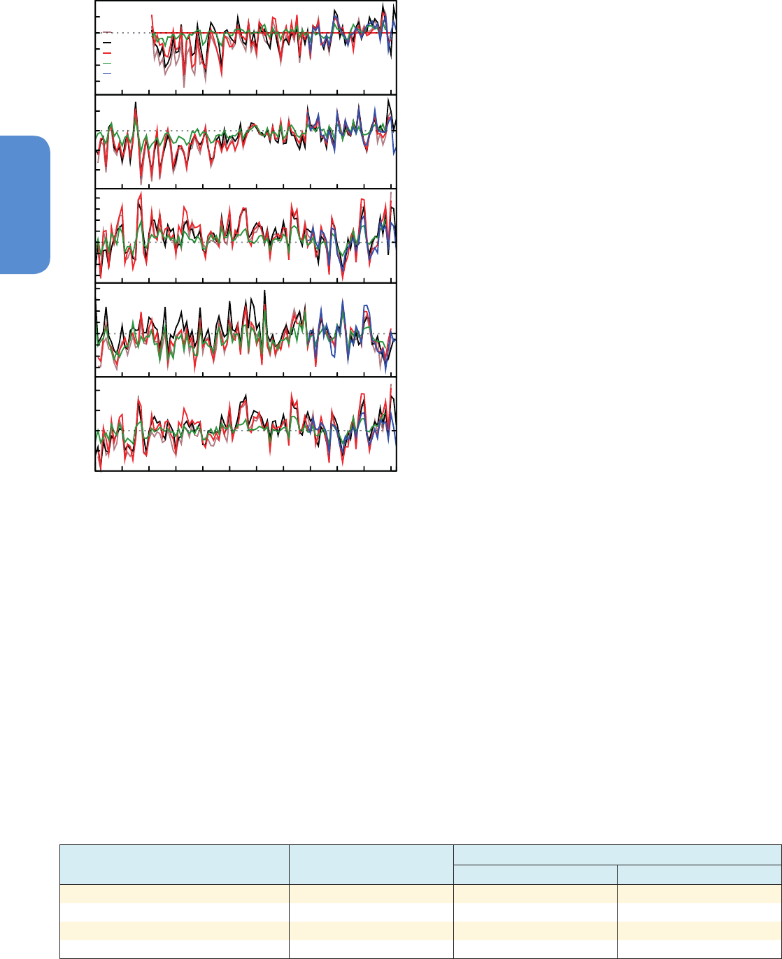
202

Chapter 2 Observations: Atmosphere and Surface

in global precipitation discussed in AR4 are uncertain, owing in part

to issues in data coverage in the early part of the 20th century (Wan

et al., 2013).

In summary, conﬁdence in precipitation change averaged over global

land areas is low for the years prior to 1950 and medium afterwards

because of insufﬁcient data, particularly in the earlier part of the record.

Available globally incomplete records show mixed and non-signiﬁcant

long-term trends in reported global mean changes. Further, when vir-

tually all the land area is ﬁlled in using a reconstruction method, the

resulting time series shows less change in land-based precipitation

since 1900.

-90

-60

-30

-60

-30

-90

-60

-30

120

Precipitation anomaly (mm yr

-1

)

-90

-60

-30

120

1900 1910 1920 1930 1940

1950 1960

1970 1980 1990 2000 2010

-60

-30

CRU

GHCN

GPCC

Smith et al.

GPCP

Global

60ºN-90ºN

30ºN-60ºN

30ºS-30ºN

60ºS-30ºS

CRU

Figure 2.28 | Annual precipitation anomalies averaged over land areas for four

latitudinal bands and the globe from ﬁve global precipitation data sets relative to a

1981–2000 climatology.

Table 2.9 | Trend estimates and 90% conﬁdence intervals (Box 2.2) for annual precipitation for each time series in Figure 2.28 over two common periods of record.

Data Set Area

Trends in mm yr

–1

per decade

1901–2008 1951–2008

CRU TS 3.10.01 (updated from Mitchell and Jones, 2005) Global 2.77 ± 1.46 –2.12 ± 3.52

GHCN V2 (updated through 2011; Vose et al., 1992) Global 2.08 ± 1.66 –2.77 ± 3.92

GPCC V6 (Becker et al., 2013) Global 1.48 ± 1.65 –1.54 ± 4.50

Smith et al. (2012) Global 1.01 ± 0.64 0.68 ± 2.07

2.5.1.2 Spatial Variability of Observed Trends

The latitude band plots in Figure 2.28 suggest that precipitation over

tropical land areas (30°S to 30°N) has increased over the last decade

reversing the drying trend that occurred from the mid-1970s to mid-

1990s. As a result the period 1951–2008 shows no signiﬁcant overall

trend in tropical land precipitation in any of the datasets (Table 2.10).

Longer term trends (1901–2008) in the tropics, shown in Table 2.10,

are also non-signiﬁcant for each of the four data sets. The mid-latitudes

of the NH (30°N to 60°N) show an overall increase in precipitation

from 1901 to 2008 with statistically signiﬁcant trends for each data

set. For the shorter period (1951–2008) the trends are also positive

but non-signiﬁcant for three of the four data sets. For the high lat-

itudes of the NH (60°N to 90°N) where data completeness permits

trend calculations solely for the 1951–2008 period, all datasets show

increases but there is a wide range of magnitudes and the inﬁlled

Smith et al. series shows small and insigniﬁcant trends (Table 2.10).

Fewer data from high latitude stations make these trends less certain

and yield low conﬁdence in resulting zonal band average estimates.

In the mid-latitudes of the SH (60°S to 30°S) there is limited evidence

of long-term increases with three data sets showing signiﬁcant trends

for the 1901–2008 period but GHCN having negative trends that are

not signiﬁcant. For the 1951–2008 period changes in SH mid-latitude

precipitation are less certain, with one data set showing a signiﬁcant

trend towards drying, two showing non-signiﬁcant drying trends and

the ﬁnal dataset suggesting increases in precipitation. All data sets

show an abrupt decline in SH mid-latitude precipitation in the early

2000s (Figure 2.28) consistent with enhanced drying that has very

recently recovered. These results for latitudinal changes are broadly

consistent with the global satellite observations for the 1979–2008

period (Allan et al., 2010) and land-based gauge measurements for the

1950–1999 period (Zhang et al., 2007a).

In AR4, maps of observed trends of annual precipitation for 1901–2005

were calculated using GHCN interpolated to a 5° × 5° latitude/longi-

tude grid. Trends (in percent per decade) were calculated for each grid

box and showed statistically signiﬁcant changes, particularly increas-

es in eastern and northwestern North America, parts of Europe and

Russia, southern South America and Australia, declines in the Sahel

region of Africa, and a few scattered declines elsewhere.

Figure 2.29 shows the spatial variability of long-term trends (1901–

2010) and more recent trends (1951–2010) over land in annual precip-

itation using the CRU, GHCN and GPCC data sets. The trends are com-

puted from land-only grid box time series using each native data set

grid resolution. The patterns of these absolute trends (in mm yr

–1

per

decade) are broadly similar to the trends (in percent per decade) relative

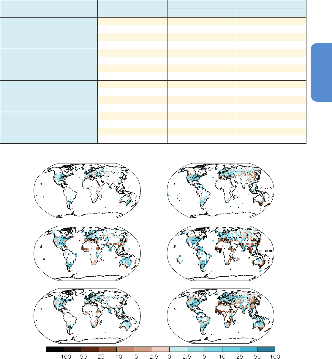
203

Observations: Atmosphere and Surface Chapter 2

Table 2.10 | Trend estimates and 90% conﬁdence intervals (Box 2.2) for annual precipitation for each time series in Figure 2.28 over two periods. Dashes indicate not enough

data available for trend calculation. For the latitudinal band 90°S to 60°S not enough data exist for each product in either period.

Data Set

Area

Trends in mm yr

–1

per decade

1901–2008 1951–2008

CRU TS 3.10.01 (updated from Mitchell and

Jones, 2005)

60°N–90°N – 5.82 ± 2.72

30°N–60°N 3.82 ± 1.14 1.13 ± 2.01

30°S–30°N 0.89 ± 2.89 –4.22 ± 8.27

60°S–30°S 3.88 ± 2.28 –3.73 ± 5.94

GHCN V2 (updated through 2011; Vose et al., 1992)

60°N–90°N – 4.52 ± 2.64

30°N–60°N 3.23 ± 1.10 1.39 ± 1.98

30°S–30°N 1.01 ± 3.00 –5.15 ± 7.28

60°S–30°S –0.57 ± 2.27 –8.01 ± 5.63

GPCC V6 (Becker et al., 2013)

60°N–90°N – 2.69 ± 2.54

30°N–60°N 3.14 ± 1.05 1.50 ± 1.93

30°S–30°N –0.48 ± 3.35 –4.16 ± 9.65

60°S–30°S 2.40 ± 2.01 –0.51 ± 5.45

Smith et al. (2012)

60°N–90°N – 0.63 ± 1.27

30°N–60°N 1.44 ± 0.50 0.97 ± 0.88

30°S–30°N 0.43 ± 1.48 0.67 ± 4.75

60°S–30°S 2.94 ± 1.40 0.78 ± 3.31

Trend (mm yr

-1

per decade)

CRU 1901-2010

GHCN 1901-2010 GHCN 1951-2010

GPCC 1901-2010 GPCC 1951-2010

CRU 1951-2010

Figure 2.29 | Trends in annual precipitation over land from the CRU, GHCN and GPCC data sets for 1901–2010 (left-hand panels) and 1951–2010 (right-hand panels). Trends

have been calculated only for those grid boxes with greater than 70% complete records and more than 20% data availability in ﬁrst and last decile of the period. White areas

indicate incomplete or missing data. Black plus signs (+) indicate grid boxes where trends are signiﬁcant (i.e., a trend of zero lies outside the 90% conﬁdence interval).

204

Chapter 2 Observations: Atmosphere and Surface

to local climatology (Supplementary Material 2.SM.6.1). Increases for

the period 1901–2010 are seen in the mid- and higher-latitudes of

both the NH and SH consistent with the reported changes for latitu-

dinal bands. At the grid box scale, statistically signiﬁcant trends occur

in most of the same areas, in each data set but are far more limited

than for temperature over a similar length period (cf. Figure 2.21). The

GPCC map shows the most areas with signiﬁcant trends. Comparing

the maps in Figure 2.29, most areas for which trends can be calculated

for both periods show similar trends between the 1901–2010 period

and the 1951–2010 period with few exceptions (e.g., South Eastern

Australia, ). Trends over shorter periods can differ from those implied

for the longest periods. For example, since the late 1980s trends in the

Sahel region have been signiﬁcantly positive (not shown).

In summary, when averaged over the land areas of the mid-latitudes

of the NH, all datasets show a likely overall increase in precipitation

(medium conﬁdence since 1901, but high conﬁdence after 1951).

For all other zones one or more of data sparsity, quality, or a lack

of quantitative agreement amongst available estimates yields low

conﬁdence in characterisation of such long-term trends in zonally

averaged precipitation. Nevertheless, changes in some more regional

or shorter-term recent changes can be quantiﬁed. It is likely there was

an abrupt decline in SH mid-latitude precipitation in the early 2000s

consistent with enhanced drying that has very recently recovered. Pre-

cipitation in the tropical land areas has increased (medium conﬁdence)

over the last decade, reversing the drying trend that occurred from the

mid-1970s to mid-1990s reported in AR4.

2.5.1.3 Changes in Snowfall

AR4 draws no conclusion on global changes in snowfall. Changes

in snowfall are discussed on a region-by-region basis, but focussed

mainly on North America and Eurasia. Statistically signiﬁcant increases

were found in most of Canada, parts of northern Europe and Russia. A

number of areas showed a decline in the number of snowfall events,

especially those where climatological averaged temperatures were

close to 0°C and where warming led to earlier onset of spring. Also,

an increase in lake-effect snowfall was found for areas near the North

American Great Lakes.

Since AR4, most published literature has considered again changes in

snowfall in North America. These studies have conﬁrmed that more

winter-time precipitation is falling as rain rather than snow in the

western USA (Knowles et al., 2006), the Paciﬁc Northwest and Central

USA (Feng and Hu, 2007). Kunkel et al. (2009) analyzed trends using

a specially quality-controlled data set of snowfall observations over

the contiguous USA and found that snowfall has been declining in the

western USA, northeastern USA and southern margins of the season-

al snow region, but increasing in the western Great Plains and Great

Lakes regions. Snowfall in Canada has increased mainly in the north

while a signiﬁcant decrease was observed in the southwestern part of

the country for 1950–2009 (Mekis and Vincent, 2011).

Other regions that have been analyzed include Japan (Takeuchi et al.,

2008), where warmer winters in the heavy snowfall areas on Honshu

are associated with decreases in snowfall and precipitation in general.

Shekar et al. (2010) found declines in total seasonal snowfall along

with increases in maximum and minimum temperatures in the west-

ern Himalaya. Serquet et al. (2011) analyzed snowfall and rainfall days

since 1961 and found the proportion of snowfall days to rainfall days

in Switzerland was declining in association with increasing temper-

atures. Scherrer and Appenzeller (2006) found a trend in a pattern

of variability of snowfall in the Swiss Alps that indicated decreasing

snow at low altitudes relative to high altitudes, but with large decadal

variability in key snow indicators (Scherrer et al., 2013). Van Ommen

and Morgan (2010) draw a link between increased snowfall in coastal

East Antarctica and increased southwest Western Australia drought.

However, Monaghan and Bromwich (2008) found an increase in snow

accumulation over all Antarctica from the late 1950s to 1990, then a

decline to 2004. Thus snowfall changes in Antarctica remain uncertain.

In summary, in most regions analyzed, it is likely that decreasing num-

bers of snowfall events are occurring where increased winter temper-

atures have been observed (North America, Europe, Southern and East

Asia). Conﬁdence is low for the changes in snowfall over Antarctica.

2.5.2 Streamﬂow and Runoff

AR4 concluded that runoff and river discharge generally increased at

high latitudes, with some exceptions. No consistent long-term trend in

discharge was reported for the world’s major rivers on a global scale.

River discharge is unique among water cycle components in that it

both spatially and temporally integrates surplus waters upstream

within a catchment (Shiklomanov et al., 2010) which makes it well

suited for in situ monitoring (Arndt et al., 2010). The most recent com-

prehensive analyses (Milliman et al., 2008; Dai et al., 2009) do not sup-

port earlier work (Labat et al., 2004) that reported an increasing trend

in global river discharge associated with global warming during the

20th century. It must be noted that many if not most large rivers, espe-

cially those for which a long-term streamﬂow record exists, have been

impacted by human inﬂuences such as dam construction or land use,

so results must be interpreted with caution. Dai et al. (2009) assem-

bled a data set of 925 most downstream stations on the largest rivers

monitoring 80% of the global ocean draining land areas and capturing

73% of the continental runoff. They found that discharges in about

one-third of the 200 largest rivers (including the Congo, Mississippi,

Yenisey, Paraná, Ganges, Colombia, Uruguay and Niger) show sta-

tistically signiﬁcant trends during 1948–2004, with the rivers having

downward trends (45) outnumbering those with upward trends (19).

Decreases in streamﬂow were found over many low and mid-latitude

river basins such as the Yellow River in northern China since 1960s

(Piao et al., 2010) where precipitation has decreased. Increases in

streamﬂow during the latter half of the 20th century also have been

reported over regions with increased precipitation, such as parts of

the USA (Groisman et al., 2004), and in the Yangtze River in southern

China (Piao et al., 2010). In the Amazon basin an increase of discharge

extremes is observed over recent decades (Espinoza Villar et al., 2009).

For France, Giuntoli et al. (2013) found that the sign of the temporal

trends in natural streamﬂows varies with period studied. In that case

study, signiﬁcant correlations between median to low ﬂows and the

Atlantic Multidecadal Oscillation (AMO; Section 2.7.8) result in long

quasi-periodic oscillations.

205

Observations: Atmosphere and Surface Chapter 2

At high latitudes, increasing winter base ﬂow and mean annual

stream ﬂow resulting from possible permafrost thawing were report-

ed in northwest Canada (St. Jacques and Sauchyn, 2009). Rising min-

imum daily ﬂows also have been observed in northern Eurasian rivers

(Smith et al., 2007). For ocean basins other than the Arctic, and for

the global ocean as a whole, the data for continental discharge show

small or downward trends, which are statistically signiﬁcant for the

Paciﬁc (–9.4 km

–1

). Precipitation is a major driver for the discharge

trends and for the large interannual-to-decadal variations (Dai et al.,

2009). However, for the Arctic drainage areas, Adam and Lettenmaier

(2008) found that upward trends in streamﬂow are not accompanied

by increasing precipitation, especially over Siberia, based on available

observations. Zhang et al. (2012a) argued that precipitation measure-

ments are sparse and exhibit large cold-season biases in the Arctic

drainage areas and hence there would be large uncertianties using

these data to investigate their inﬂuence on streamﬂow.

Recently, Stahl et al. (2010) and Stahl and Tallaksen (2012) investigat-

ed streamﬂow trends based on a data set of near-natural streamﬂow

records from more than 400 small catchments in 15 countries across

Europe for 1962–2004. A regional coherent pattern of annual stream-

ﬂow trends was revealed with negative trends in southern and eastern

regions, and generally positive trends elsewhere. Subtle regional dif-

ferences in the subannual changes in various streamﬂow metrics also

can be captured in regional studies such as by Monk et al. (2011) for

Canadian rivers.

In summary, the most recent comprehensive analyses lead to the con-

clusion that conﬁdence is low for an increasing trend in global river

discharge during the 20th century.

2.5.3 Evapotranspiration Including Pan Evaporation

AR4 concluded that decreasing trends were found in records of pan

evaporation over recent decades over the USA, India, Australia, New

Zealand, China and Thailand and speculated on the causes including

decreased surface solar radiation, sunshine duration, increased spe-

ciﬁc humidity and increased clouds. However, AR4 also reported that

direct measurements of evapotranspiration over global land areas

are scarce, and concluded that reanalysis evaporation ﬁelds are not

reliable because they are not well constrained by precipitation and

radiation.

Since AR4 gridded data sets have been developed that estimate actual

evapotranspiration from either atmospheric forcing and thermal

remote sensing, sometimes in combination with direct measurements

(e.g., from FLUXNET, a global network of ﬂux towers), or interpolation

of FLUXNET data using regression techniques, providing an unprec-

edented look at global evapotranspiration (Mueller et al., 2011). On

a global scale, evapotranspiration over land increased from the early

1980s up to the late 1990s (Wild et al., 2008; Jung et al., 2010; Wang et

al., 2010) and Wang et al. (2010) found that global evapotranspiration

increased at a rate of 0.6 W m

–2

per decade for the period 1982–2002.

After 1998, a lack of moisture availability in SH land areas, particularly

decreasing soil moisture, has acted as a constraint to further increase

of global evapotranspiration (Jung et al., 2010).

Zhang et al. (2007b) found decreasing pan evaporation at stations

across the Tibetan Plateau, even with increasing air temperature. Sim-

ilarly, decreases in pan evaporation were also found for northeast-

ern India (Jhajharia et al., 2009) and the Canadian Prairies (Burn and

Hesch, 2007). A continuous decrease in reference and pan evapora-

tion for the period 1960–2000 was reported by Xu et al. (2006a) for a

humid region in China, consistent with reported continuous increase

in aerosol levels over China (Qian et al., 2006; Section 2.2.4). Rod-

erick et al. (2007) examined the relationship between pan evapora-

tion changes and many of the possible causes listed above using a

physical model and conclude that many of the decreases (USA, China,

Tibetan Plateau, Australia) cited previously are related to declining

wind speeds and to a lesser extent decreasing solar radiation. Fu et al.

(2009) provided an overview of pan evaporation trends and conclud-

ed the major possible causes, changes in wind speed, humidity and

solar radiation, have been occurring, but that the importance of each

is regionally dependent.

The recent increase in incoming shortwave radiation in regions with

decreasing aerosol concentrations (Section 2.2.3) can explain positive

evapotranspiration trends only in the humid part of Europe. In semiarid

and arid regions, trends in evapotranspiration largely follow trends in

precipitation (Jung et al., 2010). Trends in surface winds (Section 2.7.2)

and CO

(Section 2.2.1.1.1) also alter the partitioning of available

energy into evapotranspiration and sensible heat. While surface wind

trends may explain pan evaporation trends over Australia (Rayner,

2007; Roderick et al., 2007), their impact on actual evapotranspiration

is limited due to the compensating effect of boundary-layer feedbacks

(van Heerwaarden et al., 2010). In vegetated regions, where a large

part of evapotranspiration comes from transpiration through plants’

stomata, rising CO

concentrations can lead to reduced stomatal open-

ing and evapotranspiration (Idso and Brazel, 1984; Leakey et al., 2006).

Additional regional effects that impact evapotranspiration trends are

lengthening of the growing season and land use change.

In summary, there is medium conﬁdence that pan evaporation contin-

ued to decline in most regions studied since AR4 related to changes

in wind speed, solar radiation and humidity. On a global scale, evapo-

transpiration over land increased (medium conﬁdence) from the early

1980s up to the late 1990s. After 1998, a lack of moisture availability

in SH land areas, particularly decreasing soil moisture, has acted as a

constraint to further increase of global evapotranspiration.

2.5.4 Surface Humidity

AR4 reported widespread increases in surface air moisture content

since 1976, along with near-constant relative humidity over large

scales though with some signiﬁcant changes speciﬁc to region, time

of day or season.

In good agreement with previous analysis from Dai (2006), Willett et al.

(2008) show widespread increasing speciﬁc humidity across the globe

from the homogenized gridded monthly mean anomaly product Had-

CRUH (1973–2003). Both Dai and HadCRUH products that are blended

land and ocean data products end in 2003 but HadISDH (1973–2012)

(Willett et al., 2013) and the NOCS product (Berry and Kent, 2009) are

available over the land and ocean respectively through 2012. There

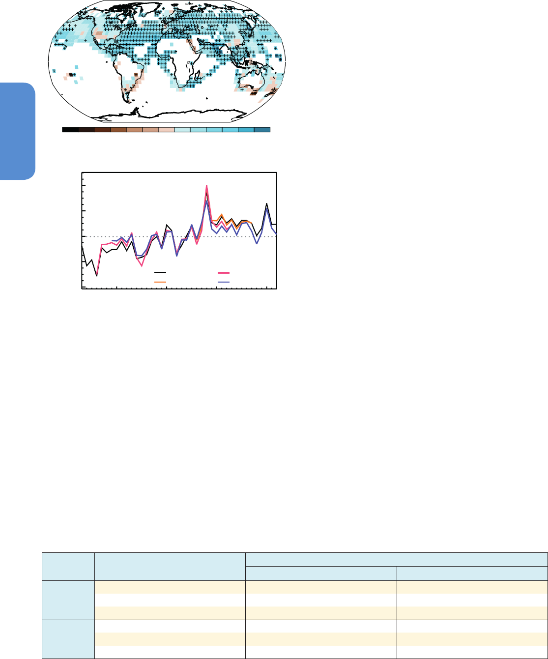
206

Chapter 2 Observations: Atmosphere and Surface

are some small isolated but coherent areas of drying over some of the

more arid land regions (Figure 2.30a). Moistening is largest in the trop-

ics and in the extratropics during summer over both land and ocean.

Large uncertainty remains over the SH where data are sparse. Global

speciﬁc humidity is sensitive to large-scale phenomena such as ENSO

(Figure 2.30b; Box 2.5). It is strongly correlated with land surface tem-

perature averages over the 23 Giorgi and Francisco (2000) regions for

the period 1973–1999 and exhibits increases mostly at or above the

1973–2012

Specific humidity anomaly (g kg

-1

)

0.4

0.2

0.0

-0.2

-0.4

1980 1990 2000 2010

-0.5 -0.25-0.2-0.15 -0.1 -0.050.0.050.1 0.15 0.20.250.5

Trend (g kg

-1

per decade)

HadISDH

ERA-InterimHadCRUH

Dai

(a)

(b)

Figure 2.30 | (a) Trends in surface speciﬁc humidity from HadISDH and NOCS over

1973–2012. Trends have been calculated only for those grid boxes with greater than

70% complete records and more than 20% data availability in ﬁrst and last decile

of the period. White areas indicate incomplete or missing data. Black plus signs (+)

indicate grid boxes where trends are signiﬁcant (i.e., a trend of zero lies outside the

90% conﬁdence interval). (b) Global annual average anomalies in land surface spe-

ciﬁc humidity from Dai (2006; red), HadCRUH (Willett et al., 2013; orange), HadISDH

(Willett et al., 2013; black), and ERA-Interim (Simmons et al., 2010; blue). Anomalies

are relative to the 1979–2003 climatology.

Table 2.11 | Trend estimates and 90% conﬁdence intervals (Box 2.2) for surface humidity over two periods.

Data Set

Trends in % per decade

1976–2003 1973–2012

Land

HadISDH (Willett et al., 2008) 0.127 ± 0.037 0.091 ± 0.023

HadCRUH_land (Willett et al., 2008) 0.128 ± 0.043

Dai_land (Dai, 2006) 0.099 ± 0.046

Ocean

NOCS (Berry and Kent, 2009) 0.114 ± 0.064 0.090 ± 0.033

HadCRUH_marine (Willett et al., 2008) 0.065 ± 0.049

Dai_marine (Dai, 2006) 0.058 ± 0.044

increase expected from the Clausius–Clapeyron relation (about 7%

°C

–1

; Annex III: Glossary) with high conﬁdence (Willett et al., 2010).

Land surface humidity trends are similar in ERA-Interim to observed

estimates of homogeneity-adjusted data sets (Simmons et al., 2010;

Figure 2.30b).

Since 2000 surface speciﬁc humidity over land has remained largely

unchanged (Figure 2.30) whereas land areas have on average warmed

slightly (Figure 2.14), implying a reduction in land region relative

humidity. This may be linked to the greater warming of the land surface

relative to the ocean surface (Joshi et al., 2008). The marine speciﬁc

humidity (Berry and Kent, 2009), like that over land, shows widespread

increases that correlate strongly with SST. However, there is a marked

decline in marine relative humidity around 1982. This is reported in Wil-

lett et al. (2008) where its origin is concluded to be a non-climatic data

issue owing to a change in reporting practice for dewpoint temperature.

In summary, it is very likely that global near surface air speciﬁc humidi-

ty has increased since the 1970s. However, during recent years the near

surface moistening over land has abated (medium conﬁdence). As a

result, fairly widespread decreases in relative humidity near the surface

are observed over the land in recent years.

2.5.5 Tropospheric Humidity

As reported in AR4, observations from radiosonde and GPS meas-

urements over land, and satellite measurements over ocean indicate

increases in tropospheric water vapour at near-global spatial scales

which are consistent with the observed increase in atmospheric tem-

perature over the last several decades. Tropospheric water vapour

plays an important role in regulating the energy balance of the surface

and TOA, provides a key feedback mechanism and is essential to the

formation of clouds and precipitation.

2.5.5.1 Radiosonde

Radiosonde humidity data for the troposphere were used sparingly

in AR4, noting a renewed appreciation for biases with the operation-

al radiosonde data that had been highlighted by several major ﬁeld

campaigns and intercomparisons. Since AR4 there have been three

distinct efforts to homogenize the tropospheric humidity records from

operational radiosonde measurements (Durre et al., 2009; McCarthy

et al., 2009; Dai et al., 2011) (Supplementary Material 2.SM.6.1, Table

2.SM.9). Over the common period of record from 1973 onwards, the

resulting estimates are in substantive agreement regarding speciﬁc

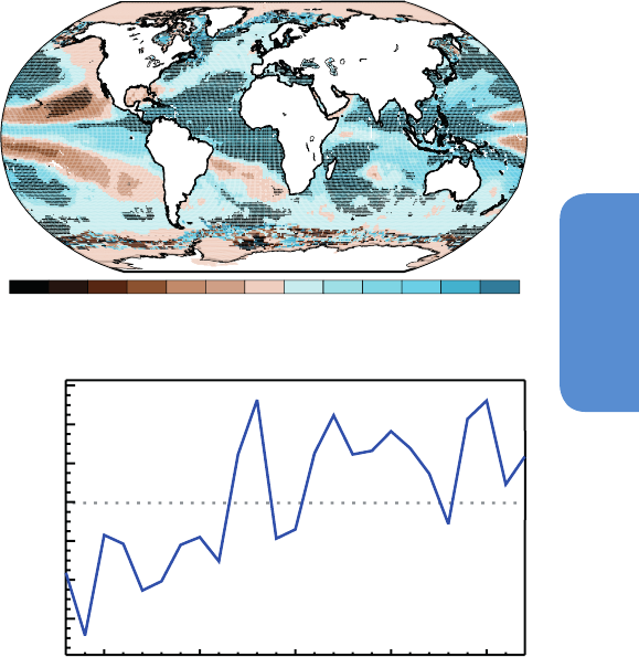
207

Observations: Atmosphere and Surface Chapter 2

humidity trends at the largest geographical scales. On average, the

impact of the correction procedures is to remove an artiﬁcial temporal

trend towards drying in the raw data and indicate a positive trend in

free tropospheric speciﬁc humidity over the period of record. In each

analysis, the rate of increase in the free troposphere is concluded to

be largely consistent with that expected from the Clausius– Clapeyron

relation (about 7% per degree Celsius). There is no evidence for a

signiﬁcant change in free tropospheric relative humidity, although

a decrease in relative humidity at lower levels is observed (Section

2.5.5). Indeed, McCarthy et al. (2009) show close agreement between

their radiosonde product at the lowest levels and HadCRUH (Willett et

al., 2008).

2.5.5.2 Global Positioning System

Since the early 1990s, estimates of column integrated water vapour

have been obtained from ground-based Global Positioning System

(GPS) receivers. An international network started with about 100

stations in 1997 and has currently been expanded to more than 500

(primarily land-based) stations. Several studies have compiled GPS

water vapour data sets for climate studies (Jin et al., 2007; Wang et

al., 2007; Wang and Zhang, 2008, 2009). Using such data, Mears et al.

(2010) demonstrated general agreement of the interannual anomalies

between ocean-based satellite and land-based GPS column integrat-

ed water vapour data. The interannual water vapour anomalies are

closely tied to the atmospheric temperature changes in a manner con-

sistent with that expected from the Clausius–Clapeyron relation. Jin

et al. (2007) found an average column integrated water vapour trend

of about 2 kg m

–2

per decade during 1994–2006 for 150 (primarily

land-based) stations over the globe, with positive trends at most NH

stations and negative trends in the SH. However, given the short length

(about 10 years) of the GPS records, the estimated trends are very sen-

sitive to the start and end years and the analyzed time period (Box 2.2).

2.5.5.3 Satellite

AR4 reported positive decadal trends in lower and upper tropospheric

water vapour based on satellite observations for the period 1988–2004.

Since AR4, there has been continued evidence for increases in lower

tropospheric water vapour from microwave satellite measurements of

column integrated water vapour over oceans (Santer et al., 2007; Wentz

et al., 2007) and globally from satellite measurements of spectrally

resolved reﬂected solar radiation (Mieruch et al., 2008). The interannual

variability and longer-term trends in column-integrated water vapour

over oceans are closely tied to changes in SST at the global scale and

interannual anomalies show remarkable agreement with low-level spe-

ciﬁc humidity anomalies from HadCRUH (O’Gorman et al., 2012). The

rate of moistening at large spatial scales over oceans is close to that

expected from the Clausius–Clapeyron relation (about 7% per degree

Celsius) with invariant relative humidity (Figure 2.31). Satellite meas-

urements also indicate that the globally averaged upper tropospheric

relative humidity has changed little over the period 1979–2010 while

the troposphere has warmed, implying an increase in the mean water

vapour mass in the upper troposphere (Shi and Bates, 2011).

Interannual variations in temperature and upper tropospheric water

vapour from IR satellite data are consistent with a constant RH

behavior at large spatial scales (Dessler et al., 2008; Gettelman and

Fu, 2008; Chung et al., 2010). On decadal time-scales, increased GHG

concentrations reduce clear-sky outgoing long-wave radiation (Allan,

2009; Chung and Soden, 2010), thereby inﬂuencing inferred relation-

ships between moisture and temperature. Using Meteosat IR radianc-

es, Brogniez et al. (2009) demonstrated that interannual variations in

free tropospheric humidity over subtropical dry regions are heavily

inﬂuenced by meridional mixing between the deep tropics and the

extra tropics. Regionally, upper tropospheric humidity changes in the

tropics were shown to relate strongly to the movement of the ITCZ

based upon microwave satellite data (Xavier et al., 2010). Shi and

Bates (2011) found an increase in upper tropospheric humidity over

the equatorial tropics from 1979 to 2008. However there was no signif-

icant trend found in tropical-mean or global-mean averages, indicating

that on these time and space scales the upper troposphere has seen

little change in relative humidity over the past 30 years. While micro-

wave satellite measurements have become increasingly relied upon for

studies of upper tropospheric humidity, the absence of a homogenized

data set across multiple satellite platforms presents some difﬁculty in

documenting coherent trends from these records (John et al., 2011).

1998 - 2012

Trend (g kg

-1

per decade)

Water vapour (kg m

-2

per decade)

1990 1995 2000 2005 2010

0.6

0.4

0.2

0.0

-0.2

-0.4

-0.6

-10 -5 -2.5 -1 -0.5 -0.250. 0.25 0.512.5 5 10

(a)

(b)

Figure 2.31 | (a) Trends in column integrated water vapour over ocean surfaces from

Special Sensor Microwave Imager (Wentz et al., 2007) for the period 1988–2010.

Trends have been calculated only for those grid boxes with greater than 70% complete

records and more than 20% data availability in ﬁrst and last decile of the period. Black

plus signs (+) indicate grid boxes where trends are signiﬁcant (i.e., a trend of zero lies

outside the 90% conﬁdence interval). (b) Global annual average anomalies in column

integrated water vapour averaged over ocean surfaces. Anomalies are relative to the

1988–2007 average.

208

Chapter 2 Observations: Atmosphere and Surface

2.5.5.4 Reanalyses

Using NCEP reanalyses for the period 1973–2007, Paltridge et al.

(2009) found negative trends in speciﬁc humidity above 850 hPa over

both the tropics and southern mid-latitudes, and above 600 hPa in the

NH mid-latitudes. However, as noted in AR4, reanalysis products suffer

from time dependent biases and have been shown to simulate unreal-

istic trends and variability over the ocean (Mears et al., 2007; John et

al., 2009) (Box 2.3). Some reanalysis products do reproduce observed

variability in low level humidity over land (Simmons et al., 2010), more

complete assesments of multiple reanalysis products yield substan-

tially different and even opposing trends in free tropospheric speciﬁc

humidity (Chen et al., 2008; Dessler and Davis, 2010). Consequently,

reanalysis products are still considered to be unsuitable for the analysis

of tropospheric water vapour trends (Sherwood et al., 2010).

In summary, radiosonde, GPS and satellite observations of tropospher-

ic water vapour indicate very likely increases at near global scales

since the 1970s occurring at a rate that is generally consistent with

the Clausius-Clapeyron relation (about 7% per degree Celsius) and

the observed increase in atmospheric temperature. Signiﬁcant trends

in tropospheric relative humidity at large spatial scales have not been

observed, with the exception of near-surface air over land where rela-

tive humidity has decreased in recent years (Section 2.5.5).

2.5.6 Clouds

2.5.6.1 Surface Observations

AR4 reported that surface-observed total cloud cover may have

increased over many land areas since the middle of the 20th centu-

ry, including the USA, the former USSR, Western Europe, mid-latitude

Canada and Australia. A few regions exhibited decreases, including

China and central Europe. Trends were less globally consistent since

the early 1970s, with regional reductions in cloud cover reported for

western Asia and Europe but increases over the USA.

Analyses since AR4 have indicated decreases in cloud occurrence/cover

in recent decades over Poland (Wibig, 2008), China and the Tibetan

Plateau (Duan and Wu, 2006; Endo and Yasunari, 2006; Xia, 2010b),

in particular for upper level clouds (Warren et al., 2007) and also over

Africa, Eurasia and in particular South America (Warren et al., 2007).

Increased frequency of overcast conditions has been reported for some

regions, such as Canada, from 1953 to 2002 (Milewska, 2004), with

no statistically signiﬁcant trends evident over Australia (Jovanovic et

al., 2011) and North America (Warren et al., 2007). A global analysis

of surface observations spanning the period 1971–2009 (Eastman and

Warren, 2012) indicates a small decline in total cloud cover of about

0.4% per decade which is largely attributed to declining mid- and

high-level cloud cover and is most prominent in the middle latitudes.

Regional variability in surface-observed cloudiness over the ocean

appeared more credible than zonal and global mean variations in AR4.

Multidecadal changes in upper-level cloud cover and total cloud cover

over particular areas of the tropical Indo-Paciﬁc Ocean were consist-

ent with island precipitation records and SST variability. This has been

extended more recently by Deser et al. (2010a), who found that an

eastward shift in tropical convection and total cloud cover from the

western to central equatorial Paciﬁc occurred over the 20th century

and attributed it to a long-term weakening of the Walker circulation

(Section 2.7.5). Eastman et al. (2011) report that, after the remov-

al of apparently spurious globally coherent variability, cloud cover

decreased in all subtropical stratocumulus regions from 1954 to 2008.

2.5.6.2 Satellite Observations

Satellite cloud observations offer the advantage of much better spa-

tial and temporal coverage compared to surface observations. How-

ever they require careful efforts to identify and correct for temporal

discontinuities in the data sets associated with orbital drift, sensor

degradation, and inter-satellite calibration differences. AR4 noted that

there were substantial uncertainties in decadal trends of cloud cover

in all satellite data sets available at the time and concluded that there

was no clear consensus regarding the decadal changes in total cloud

cover. Since AR4 there has been continued effort to assess the quality

of and develop improvements to multi-decadal cloud products from

operational satellite platforms (Evan et al., 2007; O’Dell et al., 2008;

Heidinger and Pavolonis, 2009).

Several satellite data sets offer multi-decadal records of cloud cover

(Stubenrauch et al., 2013). AR4 noted that there were discrepancies in

global cloud cover trends between ISCCP and other satellite data prod-

ucts, notably a large downward trend of global cloudiness in ISCCP

since the late 1980s which is inconsistent with PATMOS-x and surface

observations (Baringer et al., 2010). Recent work has conﬁrmed the

conclusion of AR4, that much of the downward trend in ISCCP is spuri-

ous and an artefact of changes in satellite viewing geometry (Evan et

al., 2007). An assesment of long-term variations in global-mean cloud

amount from nine different satellite data sets by Stubenrauch et al.

(2013) found differences between data sets were comparable in mag-

nitude to the interannual variability (2.5 to 3.5%). Such inconsistencies

result from differnces in sampling as well as changes in instrument

calibration and inhibit an accurate assessment of global-scale cloud

cover trends.

Satellite observations of low-level marine clouds suggest no long-term

trends in cloud liquid water path or optical properties (O’Dell et al.,

2008; Rausch et al., 2010). On regional scales, trends in cloud proper-

ties over China have been linked to changes in aerosol concentrations

(Qian et al., 2009; Bennartz et al., 2011) (Section 2.2.3).

In summary, surface-based observations show region- and height-spe-

ciﬁc variations and trends in cloudiness but there remains substantial

ambiguity regarding global-scale cloud variations and trends, especial-

ly from satellite observations. Although trends of cloud cover are con-

sistent between independent data sets in certain regions, substantial

ambiguity and therefore low conﬁdence remains in the observations of

global-scale cloud variability and trends.

2.6 Changes in Extreme Events

AR4 highlighted the importance of understanding changes in extreme

climate events (Annex III: Glossary) because of their disproportionate

209

Observations: Atmosphere and Surface Chapter 2

impact on society and ecosystems compared to changes in mean cli-

mate (see also IPCC Working Group II). More recently a comprehensive

assessment of observed changes in extreme events was undertaken by

the IPCC Special Report on Managing the Risks of Extreme Events and

Disasters to Advance Climate Change Adaptation (SREX) (Seneviratne

et al., 2012; Section 1.3.3).

Data availability, quality and consistency especially affect the statistics

of extremes and some variables are particularly sensitive to chang-

ing measurement practices over time. For example, historical tropical

cyclone records are known to be heterogeneous owing to changing

observing technology and reporting protocols (Section 14.6.1) and

when records from multiple ocean basins are combined to explore

global trends, because data quality and reporting protocols vary sub-

stantially between regions (Knapp and Kruk, 2010). Similar problems

have been discovered when analysing wind extremes, because of the

sensitivity of measurements to changing instrumentation and observ-

ing practice (e.g., Smits et al., 2005; Wan et al., 2010).

Numerous regional studies indicate that changes observed in the

frequency of extremes can be explained or inferred by shifts in the

overall probability distribution of the climate variable (Grifﬁths et al.,

2005; Ballester et al., 2010; Simolo et al., 2011). However, it should be

noted that these studies refer to counts of threshold exceedance—

frequency, duration—which closely follow mean changes. Departures

from high percentiles/return periods (intensity, severity, magnitude)

are highly sensitive to changes in the shape and scale parameters of

the distribution (Schär et al., 2004; Clark et al., 2006; Della-Marta et

al., 2007a, 2007b; Fischer and Schär, 2010) and geographical location.

Debate continues over whether variance as well as mean changes are

affecting global temperature extremes (Hansen et al., 2012; Rhines and

Huybers, 2013) as illustrated in Figure 1.8 and FAQ 2.2, Figure 1. In

the following sections the conclusions from both AR4 and SREX are

reviewed along with studies subsequent to those assessments.

2.6.1 Temperature Extremes

AR4 concluded that it was very likely that a large majority of global

land areas had experienced decreases in indices of cold extremes and

increases in indices of warm extremes, since the middle of the 20th

century, consistent with warming of the climate. In addition, global-

ly averaged multi-day heat events had likely exhibited increases over

a similar period. SREX updated AR4 but came to similar conclusions

while using the revised AR5 uncertainty guidance (Seneviratne et al.,

2012). Further evidence since then indicates that the level of conﬁ-

dence that the majority of warm and cool extremes show warming

remains high.

A large amount of evidence continues to support the conclusion that

most global land areas analysed have experienced signiﬁcant warming

of both maximum and minimum temperature extremes since about

1950 (Donat et al., 2013c). Changes in the occurrence of cold and

warm days (based on daily maximum temperatures) are generally

less marked (Figure 2.32). ENSO (Box 2.5) inﬂuences both maximum

and minimum temperature variability especially around the Paciﬁc

Rim (e.g., Kenyon and Hegerl, 2008; Alexander et al., 2009) but often

affecting cold and warm extremes differently. Different data sets using

different gridding methods and/or input data (Supplementary Mate-

rial 2.SM.7) indicate large coherent trends in temperature extremes

globally, associated with warming (Figure 2.32). The level of quality

control varies between these data sets. For example, HadEX2 (Donat

et al., 2013c) uses more rigorous quality control which leads to a

reduced station sample compared to GHCNDEX (Donat et al., 2013a)

or HadGHCND (Caesar et al., 2006). However, despite these issues

data sets compare remarkably consistently even though the station

networks vary through time (Figure 2.32; Table 2.12). Other data sets

that have assessed these indices, but cover a shorter period, also agree

very well over the period of overlapping data, e.g., HadEX (Alexander

et al., 2006) and Duke (Morak et al., 2011, 2013).

The shift in the distribution of nighttime temperatures appears great-

er than daytime temperatures although whether distribution changes

are simply linked to increases in the mean or other moments is an

active area of research (Ballester et al., 2010; Simolo et al., 2011; Donat

and Alexander, 2012; Hansen et al., 2012). Indeed, all data sets exam-

ined (Duke, GHCNDEX, HadEX, HadEX2 and HadGHCND), indicate a

faster increase in minimum temperature extremes than maximum

temperature extremes. While DTR declines have only been assessed

with medium conﬁdence (Section 2.4.1.2), conﬁdence of accelerated

increases in minimum temperature extremes compared to maximum

temperature extremes is high due to the more consistent patterns of

warming in minimum temperature extremes globally.

Regional changes in a range of climate indices are assessed in Table

2.13. These indicate likely increases across most continents in unusu-

ally warm days and nights and/or reductions in unusually cold days

and nights including frosts. Some regions have experienced close to a

doubling of the occurrence of warm and a halving of the occurrence

of cold nights, for example, parts of the Asia-Paciﬁc region (Choi et

al., 2009) and parts of Eurasia (Klein Tank et al., 2006; Donat et al.,

2013a, 2013c) since the mid-20th century. Changes in both local and

global SST patterns (Section 2.4.2) and large scale circulation patterns

(Section 2.7) have been shown to be associated with regional changes

in temperature extremes (Barrucand et al., 2008; Scaife et al., 2008;

Table 2.12 | Trend estimates and 90% conﬁdence intervals (Box 2.2) for global values of cold nights (TN10p), cold days (TX10p), warm nights (TN90p) and warm days (TX90p)

over the periods 1951–2010 and 1979–2010 (see Box 2.4, Table 1 for more information on indices).

Data Set

Trends in % per decade

TN10p TX10p TN90p TX90p

1951–2010 1979–2010 1951–2010 1979–2010 1951–2010 1979–2010 1951–2010 1979–2010

HadEX2 (Donat et al., 2013c) –3.9 ± 0.6 –4.2 ± 1.2 –2.5 ± 0.7 –4.1 ± 1.4 4.5 ± 0.9 6.8 ± 1.8 2.9 ± 1.2 6.3 ± 2.2

HadGHCND (Caesar et al., 2006) –4.5 ± 0.7 –4.0 ± 1.5 –3.3 ± 0.8 –5.0 ± 1.6 5.8 ± 1.3 8.6 ± 2.3 4.2 ± 1.8 9.4 ± 2.7

GHCNDEX (Donat et al., 2013a) –3.9 ± 0.6 –3.9 ± 1.3 –2.6 ± 0.7 –3.9 ± 1.4 4.3 ± 0.9 6.3 ± 1.8 2.9 ± 1.2 6.1 ± 2.2

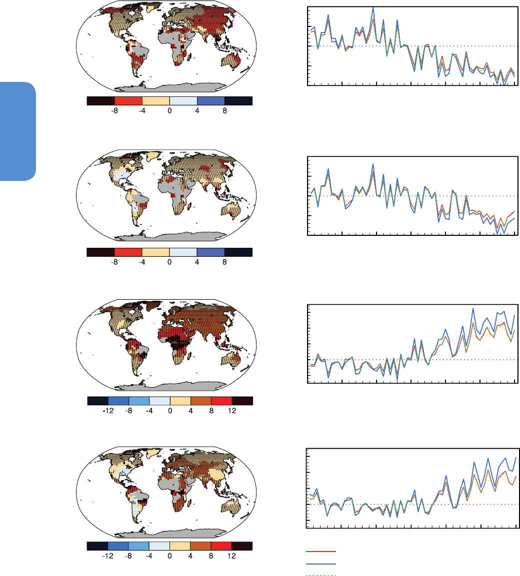
210

Chapter 2 Observations: Atmosphere and Surface

Figure 2.32 | Trends in annual frequency of extreme temperatures over the period 1951–2010, for (a) cold nights (TN10p), (b) cold days (TX10p), (c) warm nights (TN90p) and (d)

warm days (TX90p) (Box 2.4, Table 1). Trends were calculated only for grid boxes that had at least 40 years of data during this period and where data ended no earlier than 2003.

Grey areas indicate incomplete or missing data. Black plus signs (+) indicate grid boxes where trends are signiﬁcant (i.e., a trend of zero lies outside the 90% conﬁdence interval).

The data source for trend maps is HadEX2 (Donat et al., 2013c) updated to include the latest version of the European Climate Assessment data set (Klok and Tank, 2009). Beside

each map are the near-global time series of annual anomalies of these indices with respect to 1961–1990 for three global indices data sets: HadEX2 (red); HadGHCND (Caesar et

al., 2006; blue) and updated to 2010 and GHCNDEX (Donat et al., 2013a; green). Global averages are only calculated using grid boxes where all three data sets have at least 90%

of data over the time period. Trends are signiﬁcant (i.e., a trend of zero lies outside the 90% conﬁdence interval) for all the global indices shown.

Trend (days per decade)

(a) Cold Nights

(b) Cold Days

(d) Warm Days

Trend (days per decade)

-10

-20

1950 1960 1970 1980 1990 2000 2010

-10

-20

1950 1960 1970 1980 1990 2000 2010

-10

1950 1960 1970 1980 1990 2000 2010

-10

1950 1960 1970 1980 1990 2000 2010

Anomaly (days)Anomaly (days)Anomaly (days)Anomaly (days)

HadEX2

HadGHCND

GHCNDEX

211

Observations: Atmosphere and Surface Chapter 2

Region

Warm Days

(e.g., TX90p

)

Cold Days

(e.g., TX10p

)

Warm Nights

(e.g., TN90p

, TR

)

Cold Nights/Frosts

(e.g., TN10p

, FD

)

Heat Waves /

Warm Spells

Extreme

Precipitation

(e.g., RX1day

R95p

, R99p

)

Dryness (e.g,.

CDD

) / Drought

North America

and Central

America

High conﬁdence:

Likely overall

increase but spatially

varying trends

1,2

High conﬁdence:

Likely overall

decrease but

with spatially

varying trends

1,2

High conﬁdence:

Likely overall

increase

1,2

High conﬁdence:

Likely overall

decrease

1,2

Medium conﬁdence:

increases in more

regions than

decreases

1,3

but 1930s

dominates longer term

trends in the USA

High conﬁdence:

Likely overall

increase

1,2,5

but some

spatial variation

High conﬁdence:

Very likely increase

central North

America

6,7

Medium conﬁdence:

decrease

but

spatially varying

trends

High conﬁdence

Likely decrease

central North

America

South America

Medium

conﬁdence

Overall increase

Medium

conﬁdence

Overall decrease

Medium

conﬁdence

Overall increase

Medium

conﬁdence

Overall decrease

Low conﬁdence:

insufﬁcient evidence

(lack of literature)

and spatially varying

trends but some

evidence of increases

in more areas

than decreases

Medium

conﬁdence

Increases in

more regions

than decreases

8,9

but spatially

varying trends

Low conﬁdence:

limited literature

and spatially

varying trends

Europe and

Mediterranean

High conﬁdence:

Likely overall

increase

10,11,12

High conﬁdence:

Likely overall

decrease

11,12

High conﬁdence:

Likely overall

increase

11,12

High conﬁdence:

Likely overall

decrease

10,11,12

High conﬁdence

Likely increases in

most regions

3,13

High conﬁdence

b,c

Likely increases

in more regions

than decreases

5,15,16

but regional and

seasonal

variation

Medium conﬁdence:

spatially varying

trends

High conﬁdence

Likely increase in

Mediterranean

17,18

Africa and

Middle East

Low to medium

conﬁdence

b,d

limited data in

many regions but

increases in most

regions assessed

Medium

conﬁdence

increase North

Africa and

Middle East

19,20

High conﬁdence

Likely increase

southern

Africa

21,22,23

Low to medium

conﬁdence

b,d

limited data in

many regions but

decreases in most

regions assessed

Medium

conﬁdence

decrease North

Africa and

Middle East

19,20

High conﬁdence

Likely decrease

southern Africa

21,22,23

Medium

conﬁdence

b,d

limited data in

many regions but

increases in most

regions assessed

Medium

conﬁdence

increase North

Africa and

Middle East

19,20

High conﬁdence

Likely increase

southern

Africa

21,22,23

Medium

conﬁdence

b,d

limited data in

many regions but

decreases in most

regions assessed

Medium

conﬁdence

decrease North

Africa and

Middle East

19,20

High conﬁdence

Likely decrease

southern

Africa

21,22,23

Low conﬁdence

insufﬁcient evidence

(lack of literature)

Medium conﬁdence:

increase in North

Africa and

Middle East and

southern

Africa

3,19,21,22

Low conﬁdence

insufﬁcient evidence

and spatially

varying trends

Medium

conﬁdence

increases in more

regions than

decreases in

southern Africa but

spatially varying

trends depending

on index

5,21,22

Medium conﬁdence

increase

19,22,24

High conﬁdence

Likely increase in

West Africa

25,26

although 1970s

Sahel drought

dominates

the trend

Asia (excluding

South-east

Asia)

High conﬁdence

b,e

Likely overall

increase

27,28,29,30,31,32

High conﬁdence

b,e

Likely overall

decrease

27,28,29,30,31,32

High conﬁdence

b,e

Likely overall

increase

27,28,29,30,31,32

High conﬁdence

b,e

Likely overall

increase

27,28,29,30,31,32

Medium

conﬁdence

b,e

Spatially varying

trends and

insufﬁcient data

in some regions

High conﬁdence

b,c

Likely more areas

of increases than

decreases

3,28,33

Low to medium

conﬁdence

b,e

Low conﬁdence

due to insufﬁcient

evidence or spatially

varying trends.

Medium conﬁdence:

increases in more

regions than

decreases

5,34,35,36

Low to medium

conﬁdence

b,e

Medium

conﬁdence:

Increase in

eastern Asia

36,37

South-east Asia

and Oceania

High conﬁdence

b,f

Likely overall

increase

27,38,39,40

High conﬁdence

b,f

Likely overall

decrease

27,38,39

High conﬁdence

b,f

Likely overall

increase

27,38,39,40

High conﬁdence

b,f

Likely overall

decrease

27,38,39

Low conﬁdence (due

lack of literature)

to high conﬁdence

b,f

depending on region

High conﬁdence

Likely overall

increase in

Australia

3,14,41

Low conﬁdence

(lack of literature)

to high conﬁdence

b,f

High conﬁdence:

Likely decrease in

southern Australia

42,43

but index and

season dependent

Low to medium

conﬁdence

b,f

inconsistent trends

between studies

in SE Asia. Overall

increase in dryness

in southern and

eastern Australia

High conﬁdence

Likely decrease

northwest

Australia

25,26,44

Table 2.13 | Regional observed changes in a range of climate indices since the middle of the 20th century. Assessments are based on a range of ‘global’ studies and assessments

(Groisman et al., 2005; Alexander et al., 2006; Caesar et al., 2006; Shefﬁeld and Wood, 2008; Dai, 2011a, 2011b, 2013; Seneviratne et al., 2012; Shefﬁeld et al., 2012; Donat et al.,

2013a, 2013c; van der Schrier et al., 2013) and selected regional studies as indicated. Bold text indicates where the assessment is somewhat different to SREX Table 3-2. In each

such case a footnote explains why the assessment is different. See also Figures 2.32 and 2.33.

(continued on next page)

212

Chapter 2 Observations: Atmosphere and Surface

(Table 2.13 continued)

Notes:

See Table 1 in Box 2.4, for deﬁnitions.

More recent literature updates the assessment from SREX Table 3-2 (including ‘global’ studies).

This represents a measure of the area affected which is different from what was assessed in SREX Table 3-2.

This represents a slightly different region than that assessed in SREX Table 3-2 as it includes the Middle East.

This represents a slightly different region than that assessed in SREX Table 3-2 as it excludes Southeast Asia.

This represents a slightly different region than that assessed in SREX Table 3-2 as it combines SE Asia and Oceania.

Deﬁnitions for warm spells and heat waves vary (Perkins and Alexander, 2012) but here we are commonly assessing the Warm Spell Duration Index (WSDI; Zhang et al., 2011) or other heat wave

indices (e.g., HWF, HWM; (Fischer and Schär, 2010; Perkins et al., 2012) that have deﬁned multi-day heat extremes relative to either daily maximum or minimum temperatures (or both) above a

high (commonly 90th) percentile relative to a late-20th century reference period.

See Box 2.4 and Section 2.6.1 for deﬁnitions.

Kunkel et al. (2008),

Peterson et al. (2008),

Perkins et al. (2012),

Peterson et al. (2013),

Westra et al. (2013),

Groisman et al. (2012),

Villarini et al. (2013),

Skansi et al. (2013),

Haylock

et al. (2006),

Andrade et al. (2012),

Efthymiadis et al. (2011),

Moberg et al. (2006),

Della-Marta et al. (2007a),

Perkins and Alexander (2012),

Van den Besselaar et al. (2012),

Zolina

et al. (2009),

Sousa et al. (2011),

Hoerling et al. (2012),

Donat et al. (2013b),

Zhang et al. (2005),

Kruger and Sekele (2013),

New et al. (2006),

Vincent et al. (2011),

Aguilar et al.

(2009),

Dai (2013),

Shefﬁeld et al. (2012),

Choi et al. (2009),

Rahimzadeh et al. (2009),

Revadekar et al. (2012),

Tank et al. (2006),

You et al. (2010),

Zhou and Ren (2011),

Ding

et al. (2010),

Krishna Moorthy et al. (2009),

Pattanaik and Rajeevan (2010),

Wang et al. (2012b),

Fischer et al. (2011),

Caesar et al. (2011),

Chambers and Grifﬁths (2008),

Wang et

al. (2013),

Tryhorn and Risbey (2006),

Gallant et al. (2007),

King et al. (2013),

Jones et al. (2009).

Alexander et al., 2009; Li et al., 2012), particularly in regions around

the Paciﬁc Rim (Kenyon and Hegerl, 2008). Globally, there is evidence

of large-scale warming trends in the extremes of temperature, espe-

cially minimum temperature, since the beginning of the 20th century

(Donat et al., 2013c).

There are some exceptions to this large-scale warming of temperature

extremes including central North America, eastern USA (Alexander et

al., 2006; Kunkel et al., 2008; Peterson et al., 2008) and some parts of

South America (Alexander et al., 2006; Rusticucci and Renom, 2008;

Skansi et al., 2013) which indicate changes consistent with cooling in

these locations. However, these exceptions appear to be mostly associ-

ated with changes in maximum temperatures (Donat et al., 2013c). The

so-called ‘warming hole’ in central North America and eastern USA,

where temperatures have cooled relative to the signiﬁcant warming

elsewhere in the region, is associated with observed changes in the

hydrological cycle and land–atmosphere interaction (Pan et al., 2004;

Portmann et al., 2009a; Portmann et al., 2009b; Misra et al., 2012)

and decadal and multi-decadal variability linked with the Atlantic and

Paciﬁc Oceans (Meehl et al., 2012; Weaver, 2012).

Since AR4 many studies have analysed local to regional changes in

multi-day temperature extremes in more detail, speciﬁcally address-

ing different heat wave aspects such as frequency, intensity, duration

and spatial extent (Box 2.4, FAQ 2.2). Several high-proﬁle heat waves

have occurred in recent years (e.g., in Europe in 2003 (Beniston, 2004),

Australia in 2009 (Pezza et al., 2012), Russia in 2010 (Barriopedro et

al., 2011; Dole et al., 2011; Trenberth and Fasullo, 2012a) and USA in

2010/2011 (Hoerling et al., 2012) (Section 10.6.2) which have had

severe impacts (see WGII). Heat waves are often associated with qua-

si-stationary anticyclonic circulation anomalies that produce prolonged

hot conditions at the surface (Black and Sutton, 2007; Garcia-Herrera

et al., 2010), but long-term changes in the persistence of these anom-

alies are still relatively poorly understood (Section 2.7). Heat waves

can also be ampliﬁed by pre-existing dry soil conditions in transitional

climate zones (Ferranti and Viterbo, 2006; Fischer et al., 2007; Senevi-

ratne et al., 2010; Mueller and Seneviratne, 2012) and the persistence

of those soil-mositure anomalies (Lorenz et al., 2010). Dry soil-mois-

ture conditions are either induced by precipitation deﬁcits (Della-Mar-

ta et al., 2007b; Vautard et al., 2007), or evapotranspiration excesses

(Black and Sutton, 2007; Fischer et al., 2007), or a combination of both

(Seneviratne et al., 2010). This ampliﬁcation of soil moisture–temper-

ature feedbacks is suggested to have partly enhanced the duration of

extreme summer heat waves in southeastern Europe during the latter

part of the 20th century (Hirschi et al., 2011), with evidence emerging

of a signature in other moisture-limited regions (Mueller and Senevi-

ratne, 2012).

Table 2.13 shows that there has been a likely increasing trend in the

frequency of heatwaves since the middle of the 20th century in Europe

and Australia and across much of Asia where there are sufﬁcient data.

However, conﬁdence on a global scale is medium owing to lack of

studies over Africa and South America but also in part owing to dif-

ferences in trends depending on how heatwaves are deﬁned (Perkins

et al., 2012). Using monthly means as a proxy for heatwaves Coumou

et al. (2013) and Hansen et al. (2012) indicate that record-breaking

temperatures in recent decades substantially exceed what would be

expected by chance but caution is required when making inferences

between these studies and those that deal with multi-day events and/

or use more complex deﬁnitions for heatwave events. There is also

evidence in some regions that periods prior to the 1950s had more

heatwaves (e.g., over the USA, the decade of the 1930s stands out

and is also associated with extreme drought conditions (Peterson et

al., 2013) whereas conversely in other regions heatwave trends may

have been underestimated owing to poor quality and/or consistency of

data (e.g., Della-Marta et al. (2007a) over Western Europe; Kuglitsch et

al. (2009, 2010) over the Mediterranean). Recent available studies also

suggest that the number of cold spells has reduced signiﬁcantly since

the 1950s (Donat et al., 2013a, 2013c).

In summary, new analyses continue to support the AR4 and SREX

conclusions that since about 1950 it is very likely that the numbers

of cold days and nights have decreased and the numbers of warm

days and nights have increased overall on the global scale, that is, for

land areas with sufﬁcient data. It is likely that such changes have also

occurred across most of North America, Europe, Asia and Australia.

There is low to medium conﬁdence in historical trends in daily

temperature extremes in Africa and South America as there is either

213

Observations: Atmosphere and Surface Chapter 2

insufﬁcient data or trends vary across these regions. This, combined

with issues with deﬁning events, leads to the assessment that there

is medium conﬁdence that globally the length and frequency of warm

spells, including heat waves, has increased since the middle of the 20th

century although it is likely that heatwave frequency has increased

during this period in large parts of Europe, Asia and Australia.

2.6.2 Extremes of the Hydrological Cycle

In Section 2.5 mean state changes in different aspects of the hydrolog-

ical cycle are discussed. In this section we focus on the more extreme

aspects of the cycle including extreme rainfall, severe local weather

events like hail, ﬂooding and droughts. Extreme events associated with

tropical and extratropical storms are discussed in Sections 2.6.3 and

2.6.4 respectively.

2.6.2.1 Precipitation Extremes

AR4 concluded that substantial increases are found in heavy precipi-

tation events. It was likely that annual heavy precipitation events had

disproportionately increased compared to mean changes between

1951 and 2003 over many mid-latitude regions, even where there had

been a reduction in annual total precipitation. Rare precipitation (such

as the highest annual daily precipitation total) events were likely to

have increased over regions with sufﬁcient data since the late 19th

century. SREX supported this view, as have subsequent analyses, but

noted large spatial variability within and between regions (Table 3.2 of

Seneviratne et al., 2012).

Given the diverse climates across the globe, it has been difﬁcult to pro-

vide a universally valid deﬁnition of ‘extreme precipitation’. However,

Box 2.4 Table 1 indicates some of the common deﬁnitions that are used

in the scientiﬁc literature. In general, statistical tests indicate changes

in precipitation extremes are consistent with a wetter climate (Sec-

tion 7.6.5), although with a less spatially coherent pattern of change

than temperature, in that there are large areas that show increasing

trends and large areas that show decreasing trends and a lower level

of statistical signiﬁcance than for temperature change (Alexander et

al., 2006; Donat et al., 2013a, 2013c). Using R95p and SDII indices (Box

2.4), Figures 2.33a and 2.33b show these areas for heavy precipitation

amounts and precipitation intensity where sufﬁcient data are available

in the HadEX2 data set (Donat et al., 2013c) although there are more

areas showing signiﬁcant increases than decreases. Although chang-

es in large-scale circulation patterns have a substantial inﬂuence on

precipitation extremes globally (Alexander et al., 2009; Kenyon and

Hegerl, 2010), Westra et al. (2013) showed, using in situ data over land,

that trends in the wettest day of the year indicate more increases than

would be expected by chance. Over the tropical oceans satellite meas-

urements show an increase in the frequency of the heaviest rainfall

during warmer (El Niño) years (Allan and Soden, 2008).

Regional trends in precipitation extremes since the middle of the 20th

century are varied (Table 2.13). In most continents conﬁdence in trends

is not higher than medium except in North America and Europe where

there have been likely increases in either the frequency or intensity of

heavy precipitation. This assessment increases to very likely for cen-

tral North America. For North America it is also likely that increases

have occurred during the whole of the 20th century (Pryor et al., 2009;

Donat et al., 2013c; Villarini et al., 2013). For South America the most

recent integrative studies indicate heavy rain events are increasing in

frequency and intensity over the contient as a whole (Donat et al.,

2013c; Skansi et al., 2013). For Europe and the Mediterranean, the

assessment masks some regional and seasonal variation. For example,

much of the increase reported in Table 2.13 is found in winter although

with decreasing trends in some other regions such as northern Italy,

Poland and some Mediterranean coastal sites (Pavan et al., 2008; Lupi-

kasza, 2010; Toreti et al., 2010). There are mixed regional trends across

Asia and Oceania but with some indication that increases are being

observed in more regions than decreases while recent studies focused

on Africa, in general, have not found signiﬁcant trends in extreme pre-

cipitation (see Chapter 14 for more on regional variations and trends).

The above studies generally use indices which reﬂect ‘moderate’

extremes, for example, events occurring as often as 5% or 10% of the

time (Box 2.4). Only a few regions have sufﬁcient data to assess trends

in rarer precipitation events reliably, for example, events occurring on

average once in several decades. Using Extreme Value Theory, DeGae-

tano (2009) showed a 20% reduction in the return period for extreme

precipitation events over large parts of the contiguous USA from 1950

to 2007. For Europe from 1951 to 2010, Van den Besselaar et al. (2012)

reported a median reduction in 5- to 20-year return periods of 21%,

with a range between 2% and 58% depending on the subregion and

season. This decrease in return times for rare extremes is qualitatively

similar to the increase in moderate extremes for these regions reported

above, and also consistent with earlier local results for the extreme tail

of the distribution reported in AR4.

The aforementioned studies refer to daily precipitation extremes,

although rainfall will often be limited to part of the day only. The litera-

ture on sub-daily scales is too limited for a global assessment although

it is clear that analysis and framing of questions regarding sub-daily

precipitation extremes is becoming more critical (Trenberth, 2011).

Available regional studies have shown results that are even more com-

plex than for daily precipitation and with variations in the spatial pat-

terns of trends depending on event formulation and duration. However,

regional studies show indications of more increasing than decreasing

trends (Sen Roy, 2009; for India) (Sen Roy and Rouault, 2013; for South

Africa) (Westra and Sisson, 2011; for Australia). Some studies present

evidence of scaling of sub-daily precipitation with temperature that

is outside that expected from the Clausius–Clapeyron relation (about

per degree Celsius) (Lenderink and Van Meijgaard, 2008; Haerter

et al., 2010; Jones et al., 2010; Lenderink et al., 2011; Utsumi et al.,

2011), but scaling beyond that expected from thermodynamic theories

is controversial (Section 7.6.5).

In summary, further analyses continue to support the AR4 and SREX

conclusions that it is likely that since 1951 there have been statistically

signiﬁcant increases in the number of heavy precipitation events (e.g.,

above the 95th percentile) in more regions than there have been sta-

tistically signiﬁcant decreases, but there are strong regional and sub-

regional variations in the trends. In particular, many regions present

statistically non-signiﬁcant or negative trends, and, where seasonal

changes have been assessed, there are also variations between seasons

(e.g., more consistent trends in winter than in summer in Europe). The

214

Chapter 2 Observations: Atmosphere and Surface

overall most consistent trends towards heavier precipitation events are

found in central North America (very likely increase) but assessment for

Europe shows likely increases in more regions than decreases.

2.6.2.2 Floods

AR4 WGI Chapter 3 (Trenberth et al., 2007) did not assess changes in

ﬂoods but AR4 WGII concluded that there was not a general global

trend in the incidence of ﬂoods (Kundzewicz et al., 2007). SREX went

further to suggest that there was low agreement and thus low conﬁ-

dence at the global scale regarding changes in the magnitude or fre-

quency of ﬂoods or even the sign of changes.

AR5 WGII assesses ﬂoods in regional detail accounting for the fact

that trends in ﬂoods are strongly inﬂuenced by changes in river man-

agement (see also Section 2.5.2). Although the most evident ﬂood

trends appear to be in northern high latitudes, where observed warm-

ing trends have been largest, in some regions no evidence of a trend

in extreme ﬂooding has been found, for example, over Russia based

on daily river discharge (Shiklomanov et al., 2007). Other studies for

Europe (Hannaford and Marsh, 2008; Renard et al., 2008; Petrow and

Merz, 2009; Stahl et al., 2010) and Asia (Jiang et al., 2008; Delgado

et al., 2010) show evidence for upward, downward or no trend in the

magnitude and frequency of ﬂoods, so that there is currently no clear

and widespread evidence for observed changes in ﬂooding except for

the earlier spring ﬂow in snow-dominated regions (Seneviratne et al.,

2012).

In summary, there continues to be a lack of evidence and thus low con-

ﬁdence regarding the sign of trend in the magnitude and/or frequency

of ﬂoods on a global scale.

2.6.2.3 Droughts

AR4 concluded that droughts had become more common, especial-

ly in the tropics and sub-tropics since about 1970. SREX provided a

comprehensive assessment of changes in observed droughts (Section

3.5.1 and Box 3.3 of SREX), updated the conclusions provided by AR4

and stated that the type of drought considered and the complexities

in deﬁning drought (Annex III: Glossary) can substantially affect the

conclusions regarding trends on a global scale (Chapter 10). Based on

evidence since AR4, SREX concluded that there were not enough direct

observations of dryness to suggest high conﬁdence in observed trends

globally, although there was medium conﬁdence that since the 1950s

some regions of the world have experienced more intense and longer

droughts. The differences between AR4 and SREX are due primarily to

analyses post-AR4, differences in how both assessments considered

drought and updated IPCC uncertainty guidance.

There are very few direct measurements of drought related variables,

such as soil moisture (Robock et al., 2000), so drought proxies (e.g.,

PDSI, SPI, SPEI; Box 2.4) and hydrological drought proxies (e.g., Vidal

et al., 2010; Dai, 2011b) are often used to assess drought. The chosen

proxy (e.g., precipitation, evapotranspiration, soil moisture or stream-

ﬂow) and time scale can strongly affect the ranking of drought events

(Shefﬁeld et al., 2009; Vidal et al., 2010). Analyses of these indirect

indices come with substantial uncertainties. For example, PDSI may not

be comparable across climate zones. A self-calibrating (sc-) PDSI can

replace the ﬁxed empirical constants in PDSI with values representa-

tive of the local climate (Wells et al., 2004). Furthermore, for studies

using simulated soil moisture, the type of potential evapotranspiration

model used can lead to signiﬁcant differences in the estimation of the

regions affected and the areal extent of drought (Shefﬁeld et al., 2012),

but the overall effect of a more physically realistic parameterisation is

debated (van der Schrier et al., 2013).

Because drought is a complex variable and can at best be incompletely

represented by commonly used drought indices, discrepancies in the

interpretation of changes can result. For example, Shefﬁeld and Wood

(2008) found decreasing trends in the duration, intensity and severity

of drought globally. Conversely, Dai (2011a,b) found a general global

increase in drought, although with substantial regional variation and

individual events dominating trend signatures in some regions (e.g.,

the 1970s prolonged Sahel drought and the 1930s drought in the USA

and Canadian Prairies). Studies subsequent to these continue to pro-

vide somewhat different conclusions on trends in global droughts and/

or dryness since the middle of the 20th century (Shefﬁeld et al., 2012;

Dai, 2013; Donat et al., 2013c; van der Schrier et al., 2013).

Van der Schrier et al. (2013), using monthly sc-PDSI, found no strong

case either for notable drying or moisture increase on a global scale

over the periods 1901–2009 or 1950–2009, and this largely agrees

with the results of Shefﬁeld et al. (2012) over the latter period. A

comparison between the sc-PDSI calculated by van der Schrier et al.

(2013) and that of Dai (2011a) shows that the dominant mode of

variability is very similar, with a temporal evolution suggesting a trend

toward drying. However, the same analysis for the 1950–2009 period

shows an initial increase in drying in the Van der Schrier et al. data set,

followed by a decrease from the mid-1980s onwards, while the Dai

data show a continuing increase until 2000. The difference in trends

between the sc-PDSI data set of Van der Schrier et al. and Dai appears

to be due to the different calibration periods used, the shorter 1950–

1979 period in the latter study resulting in higher index values from

1980 onwards, although the associated spatial patterns are similar. In

addition, the observed precipitation forcing data set differs between

studies, with van der Schrier et al. (2013) and Shefﬁeld et al. (2012)

using CRU TS 3.10.01 (updated from Mitchell and Jones, 2005). This

data set uses fewer stations and has been wetter than some other

precipitation products in the last couple of decades (Figure 2.29,

Table 2.9), although the best data set to use is still an open question.

Despite this, a measure of sc-PDSI with potential evapotranspiration

estimated using the Penman–Montieth equation shows an increase

in the percentage of land area in drought since 1950 (Shefﬁeld et

al., 2012; Dai, 2013), while van der Schrier et al. (2013) also ﬁnds a

slight increase in the percentage of land area in severe drought using

the same measure. This is qualitatively consistent with the trends

in surface soil moisture found for the shorter period 1988–2010 by

Dorigo et al. (2012) using a new multi-satellite data set and changes

in observed streamﬂow (Dai, 2011b). However all these studies draw

somewhat different conclusions and the compelling arguments both

for (Dai, 2011b, 2013) and against (Shefﬁeld et al., 2012; van der

Schrier et al., 2013) a signiﬁcant increase in the land area experienc-

ing drought has hampered global assessment.

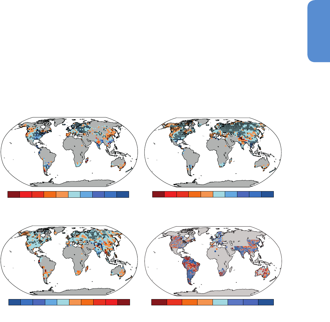
215

Observations: Atmosphere and Surface Chapter 2

Studies that support an increasing trend towards the land area affect-

ed by drought seem to be at odds with studies that look at trends

in dryness (i.e., lack of rainfall). For example, Donat et al. (2013c)

found that the annual maximum number of consecutive dry days

has declined since the 1950s in more regions than it has increased

(Figure 2.33c). However, only regions in Russia and the USA indicate

signiﬁcant changes and there is a lack of information for this index

over large regions, especially Africa. Most other studies focussing on

global dryness ﬁnd similar results, with decadal variability dominating

longer-term trends (Frich et al., 2002; Alexander et al., 2006; Donat et

al., 2013a). However, Giorgi et al. (2011) indicate that ‘hydroclimatic

intensity’ (Box 2.4, Chapter 7), a measure which combines both dry

spell length and precipitation intensity, has increased over the latter

part of the 20th century in response to a warming climate. They show

that positive trends (reﬂecting an increase in the length of drought

and/or extreme precipitation events) are most marked in Europe,

India, parts of South America and East Asia although trends appear to

have decreased (reﬂecting a decrease in the length of drought and/or

extreme precipitation events) in Australia and northern South America

(Figure 2.33c). Data availability, quality and length of record remain

issues in drawing conclusions on a global scale, however.

Despite differences between the conclusions drawn by global studies,

there are some areas in which they agree. Table 2.13 indicates that

there is medium conﬁdence of an increase in dryness or drought in East

Asia with high conﬁdence that this is the case in the Mediterannean

and West Africa. There is also high conﬁdence of decreases in dryness

or drought in central North America and north-west Australia.

In summary, the current assessment concludes that there is not enough

evidence at present to suggest more than low conﬁdence in a glob-

al-scale observed trend in drought or dryness (lack of rainfall) since the

middle of the 20th century, owing to lack of direct observations, geo-

graphical inconsistencies in the trends, and dependencies of inferred

trends on the index choice. Based on updated studies, AR4 conclusions

regarding global increasing trends in drought since the 1970s were

probably overstated. However, it is likely that the frequency and inten-

sity of drought has increased in the Mediterranean and West Africa

and decreased in central North America and north-west Australia since

1950.

Figure 2.33 | Trends in (a) annual amount of precipitation from days >95th percentile (R95p), (b) daily precipitation intensity (SDII) and (c) frequency of the annual maximum

number of consecutive dry days (CDD) (Box 2.4, Table 1). Trends are shown as relative values for better comparison across different climatic regions. Trends were calculated only

for grid boxes that had at least 40 years of data during this period and where data ended no earlier than 2003. Grey areas indicate incomplete or missing data. Black plus signs

(+) indicate grid boxes where trends are signiﬁcant (i.e., a trend of zero lies outside the 90% conﬁdence interval). The data source for trend maps is HadEX2 (Donat et al., 2013a)

updated to include the latest version of the European Climate Assessment data set (Klok and Tank, 2009). (d) Trends (normalized units) in hydroclimatic intensity (HY-INT: a multipli-

cative measure of length of dry spell and precipitation intensity) over the period 1976–2000 (adapted from Giorgi et al., 2011). An increase (decrease) in HY-INT reﬂects an increase

(decrease) in the length of drought and /or extreme precipitation events.

(b) SDII 1951-2010

Trend (% per decade)

(a) R95p 1951-2010

Trend (% per decade)

(d) HY-INT 1976-2000

-0.8 - 0.4 -0.2 0 0.2 0.4 0.8

Trend (% per decade)

-10 -5 0510 15-15-20 20

Trend (Normalised units)

-10 -5 0510 15-15-20 20

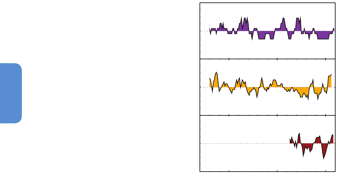
216

Chapter 2 Observations: Atmosphere and Surface

2.6.2.4 Severe Local Weather Events

Another extreme aspect of the hydrological cycle is severe local

weather phenomena such as hail or thunder storms. These are not well

observed in many parts of the world because the density of surface

meteorological observing stations is too coarse to measure all such

events. Moreover, homogeneity of existing reporting is questionable

(Verbout et al., 2006; Doswell et al., 2009). Alternatively, measures of

severe thunderstorms or hailstorms can be derived by assessing the

environmental conditions that are favourable for their formation but

this method is very uncertain (Seneviratne et al., 2012). SREX high-

lighted studies such as those of Brooks and Dotzek (2008), who found

signiﬁcant variability but no clear trend in the past 50 years in severe

thunderstorms in a region east of the Rocky Mountains in the USA,

Cao (2008), who found an increasing frequency of severe hail events in

Ontario, Canada during the period 1979–2002 and Kunz et al. (2009),

who found that hail days signiﬁcantly increased during the period

1974–2003 in southwest Germany. Hailpad studies from Italy (Eccel et

al., 2012) and France (Berthet et al., 2011) suggest slight increases in

larger hail sizes and a correlation between the fraction of precipitation

falling as hail with average summer temperature while in Argentina

between 1960 and 2008 the annual number of hail events was found

to be increasing in some regions and decreasing in others (Mezher et

al., 2012). In China between 1961 and 2005, the number of hail days

has been found to generally decrease, with the highest occurrence

between 1960 and 1980 but with a sharp drop since the mid-1980s

(CMA, 2007; Xie et al., 2008). However, there is little consistency in hail

size changes in different regions of China since 1980 (Xie et al., 2010).

Remote sensing offers a potential alterative to surface-based meteor-

ological networks for detecting changes in small scale severe weather

phenomenon such as proxy measurements of lightning from satel-

lites (Zipser et al., 2006) but there remains little convincing evidence

that changes in severe thunderstorms or hail have occurred since the

middle of the 20th century (Brooks, 2012).

In summary, there is low conﬁdence in observed trends in small-scale

severe weather phenomena such as hail and thunderstorms because

of historical data inhomogeneities and inadequacies in monitoring

systems.

2.6.3 Tropical Storms

AR4 concluded that it was likely that an increasing trend had occurred

in intense tropical cyclone activity since 1970 in some regions but that

there was no clear trend in the annual numbers of tropical cyclones.

Subsequent assessments, including SREX and more recent literature

indicate that it is difﬁcult to draw ﬁrm conclusions with respect to the

conﬁdence levels associated with observed trends prior to the satellite

era and in ocean basins outside of the North Atlantic.

Section 14.6.1 discusses changes in tropical storms in detail. Current data

sets indicate no signiﬁcant observed trends in global tropical cyclone

frequency over the past century and it remains uncertain whether any

reported long-term increases in tropical cyclone frequency are robust,

after accounting for past changes in observing capabilities (Knutson

et al., 2010). Regional trends in tropical cyclone frequency and the fre-

quency of very intense tropical cyclones have been identiﬁed in the

North Atlantic and these appear robust since the 1970s (Kossin et al.

2007) (very high conﬁdence). However, argument reigns over the cause

of the increase and on longer time scales the ﬁdelity of these trends

is debated (Landsea et al., 2006; Holland and Webster, 2007; Land-

sea, 2007; Mann et al., 2007b) with different methods for estimating

undercounts in the earlier part of the record providing mixed conclu-

sions (Chang and Guo, 2007; Mann et al., 2007a; Kunkel et al., 2008;

Vecchi and Knutson, 2008, 2011). No robust trends in annual numbers

of tropical storms, hurricanes and major hurricanes counts have been

identiﬁed over the past 100 years in the North Atlantic basin. Measures

of land-falling tropical cyclone frequency (Figure 2.34) are generally

considered to be more reliable than counts of all storms which tend

to be strongly inﬂuenced by those that are weak and/or short lived.

Callaghan and Power (2011) ﬁnd a statistically signiﬁcant decrease

in Eastern Australia land-falling tropical cyclones since the late 19th

century although including 2010/2011 season data this trend becomes

non-signiﬁcant (i.e., a trend of zero lies just inside the 90% conﬁdence

interval). Signiﬁcant trends are not found in other oceans on shorter

time scales (Chan and Xu, 2009; Kubota and Chan, 2009; Mohapatra

et al., 2011; Weinkle et al., 2012), although Grinsted et al. (2012) ﬁnd

a signiﬁcant positive trend in eastern USA using tide-guage data from

1923–2008 as a proxy for storm surges associated with land-falling

hurricanes. Differences between tropical cyclone studies highlight the

challenges that still lie ahead in assessing long-term trends.

(b)

(c)

(a)

1900

1950

2000

Landfalling Tropical Cyclones, Eastern Australia

Landfalling Hurricanes, United States

Landfalling Typhoons, China

Normalized units Normalized units Normalized units

Figure 2.34 | Normalized 5-year running means of the number of (a) adjusted land

falling eastern Australian tropical cyclones (adapted from Callaghan and Power (2011)

and updated to include 2010//2011 season) and (b) unadjusted land falling U.S. hur-

ricanes (adapted from Vecchi and Knutson (2011) and (c) land-falling typhoons in China

(adapted from CMA, 2011). Vertical axis ticks represent one standard deviation, with all

series normalized to unit standard deviation after a 5-year running mean was applied.

217

Observations: Atmosphere and Surface Chapter 2

Arguably, storm frequency is of limited usefulness if not considered

in tandem with intensity and duration measures. Intensity measures

in historical records are especially sensitive to changing technology

and improving methodology. However, over the satellite era, increases

in the intensity of the strongest storms in the Atlantic appear robust

(Kossin et al., 2007; Elsner et al., 2008) but there is limited evidence

for other regions and the globe. Time series of cyclone indices such

as power dissipation, an aggregate compound of tropical cyclone

frequency, duration and intensity that measures total wind energy

by tropical cyclones, show upward trends in the North Atlantic and

weaker upward trends in the western North Paciﬁc since the late 1970s

(Emanuel, 2007), but interpretation of longer-term trends is again con-

strained by data quality concerns (Landsea et al., 2011).

In summary, this assessment does not revise the SREX conclusion of

low conﬁdence that any reported long-term (centennial) increases in

tropical cyclone activity are robust, after accounting for past changes

in observing capabilities. More recent assessments indicate that it is

unlikely that annual numbers of tropical storms, hurricanes and major

hurricanes counts have increased over the past 100 years in the North

Atlantic basin. Evidence, however, is for a virtually certain increase in

the frequency and intensity of the strongest tropical cyclones since the

1970s in that region.

2.6.4 Extratropical Storms

AR4 noted a likely net increase in frequency/intensity of NH extreme

extratropical cyclones and a poleward shift in storm tracks since the

1950s. SREX further consolidated the AR4 assessment of poleward

shifting storm tracks, but revised the assessment of the conﬁdence

levels associated with regional trends in the intensity of extreme extra-

tropical cyclones.

Studies using reanalyses continue to support a northward and eastward

shift in the Atlantic cyclone activity during the last 60 years with both

more frequent and more intense wintertime cyclones in the high-lati-

tude Atlantic (Schneidereit et al., 2007; Raible et al., 2008; Vilibic and

Sepic, 2010) and fewer in the mid-latitude Atlantic (Wang et al., 2006b;

Raible et al., 2008). Some studies show an increase in intensity and

number of extreme Atlantic cyclones (Paciorek et al., 2002; Lehmann

et al., 2011) while others show opposite trends in eastern Paciﬁc and

North America (Gulev et al., 2001). Comparisons between studies are

hampered because of the sensitivities in identiﬁcation schemes and/

or different deﬁnitions for extreme cyclones (Ulbrich et al., 2009; Neu

et al., 2012). The ﬁdelity of research ﬁndings also rests largely with

the underlying reanalyses products that are used (Box 2.3). See also

Section 14.6.2.

Over longer periods studies of severe storms or storminess have been

performed for Europe where long running in situ pressure and wind

observations exist. Direct wind speed measurements, however, either

have short records or are hampered by inconsistencies due to changing

instrumentation and observing practice over time (Smits et al., 2005;

Wan et al., 2010). In most cases, therefore wind speed or storminess

proxies are derived from in situ pressure measurements or reanalyses

data, the quality and consistency of which vary. In situ observations

indicate no clear trends over the past century or longer (Hanna et al.,

2008; Matulla et al., 2008; Allan et al., 2009; Barring and Fortuniak,

2009), with substantial decadal and longer ﬂuctuations but with some

regional and seasonal trends (Wang et al., 2009c, 2011). Figure 2.35

shows some of these changes for boreal winter using geostrophic wind

speeds indicating that decreasing trends outnumber increasing trends

(Wang et al., 2011), although with few that are statistically signiﬁcant.

Although Donat et al. (2011) and Wang et al. (2012h) ﬁnd signiﬁcant

increases in both the strength and frequency of wintertime storms for

large parts of Europe using the 20CR (Compo et al., 2011), there is

debate over whether this is an artefact of the changing number of

assimilated observations over time (Cornes and Jones, 2011; Krueger

et al., 2013) even though Wang et al. (2012h) ﬁnd good agreement

between the 20CR trends and those derived from geostropic wind

extremes in the North Sea region.

SREX noted that available studies using reanalyses indicate a decrease

in extratropical cyclone activity (Zhang et al., 2004) and intensity

(Zhang et al., 2004; Wang et al., 2009d) over the last 50 years has been

reported for northern Eurasia (60°N to 40°N) linked to a possible north-

ward shift with increased cyclone frequency in the higher latitudes and

decrease in the lower latitudes. The decrease at lower latitudes was

also found in East Asia (Wang et al., 2012h) and is also supported by a

study of severe storms by Zou et al. (2006b) who used sub-daily in situ

pressure data from a number of stations across China.

SREX also notes that, based on reanalyses, North American cyclone

numbers have increased over the last 50 years, with no statistically

signiﬁcant change in cyclone intensity (Zhang et al., 2004). Hourly

SLP data from Canadian stations showed that winter cyclones have

become signiﬁcantly more frequent, longer lasting, and stronger in

the lower Canadian Arctic over the last 50 years (1953–2002), but

less frequent and weaker in the south, especially along the southeast

and southwest Canadian coasts (Wang et al., 2006a). Further south, a

tendency toward weaker low-pressure systems over the past few dec-

ades was found for U.S. east coast winter cyclones using reanalyses,

but no statistically signiﬁcant trends in the frequency of occurrence of

systems (Hirsch et al., 2001).

Using the 20CR (Compo et al., 2011), Wang et al. (2012h) found sub-

stantial increases in extratropical cyclone activity in the SH (20°S to

90°S). However, for southeast Australia, a decrease in activity is found

and this agrees well with geostrophic wind extremes derived from

in situ surface pressure observations (Alexander et al., 2011). This

strengthens the evidence of a southward shift in storm tracks previous-

ly noted using older reanalyses products (Fyfe, 2003; Hope et al., 2006).

Frederiksen and Frederiksen (2007) linked the reduction in cyclogenesis

at 30°S and southward shift to a decrease in the vertical mean meridi-

onal temperature gradient. There is some inconsistency among reanal-

ysis products for the SH regarding trends in the frequency of intense

extratropical cyclones (Lim and Simmonds, 2007; Pezza et al., 2007;

Lim and Simmonds, 2009) although studies tend to agree on a trend

towards more intense systems, even when inhomogeneities associated

with changing numbers of observations have been taken into account

(Wang et al., 2012h). However, further undetected contamination of

these trends owing to issues with the reanalyses products cannot be

ruled out (Box 2.3) and this lowers our conﬁdence in long-term trends.

Links between extratropical cyclone activity and large-scale variability

are discussed in Sections 2.7 and 14.6.2.

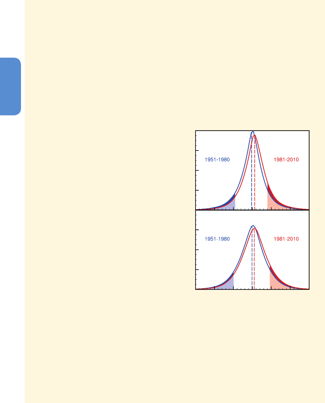
218

Chapter 2 Observations: Atmosphere and Surface

Frequently Asked Questions

FAQ 2.2 | Have There Been Any Changes in Climate Extremes?

There is strong evidence that warming has lead to changes in temperature extremes—including heat waves—since

the mid-20th century. Increases in heavy precipitation have probably also occurred over this time, but vary by

region. However, for other extremes, such as tropical cyclone frequency, we are less certain, except in some limited

regions, that there have been discernable changes over the observed record.

From heat waves to cold snaps or droughts to ﬂooding rains, recording and analysing climate extremes poses

unique challenges, not just because these events are rare, but also because they invariably happen in conjunction

with disruptive conditions. Furthermore, there is no consistent deﬁnition in the scientiﬁc literature of what consti-

tutes an extreme climatic event, and this complicates comparative global assessments.

Although, in an absolute sense, an extreme climate event will vary from place to place—a hot day in the tropics,

for instance, may be a different temperature to a hot day in the mid-latitudes—international efforts to monitor

extremes have highlighted some signiﬁcant global changes.

For example, using consistent deﬁnitions for cold

(<10th percentile) and warm (>90th percentile) days

and nights it is found that warm days and nights have

increased and cold days and nights have decreased for

most regions of the globe; a few exceptions being cen-

tral and eastern North America, and southern South

America but mostly only related to daytime tempera-

tures. Those changes are generally most apparent in

minimum temperature extremes, for example, warm

nights. Data limitations make it difﬁcult to establish

a causal link to increases in average temperatures,

but FAQ 2.2, Figure 1 indicates that daily global tem-

perature extremes have indeed changed. Whether

these changes are simply associated with the average

of daily temperatures increasing (the dashed lines in

FAQ 2.2, Figure 1) or whether other changes in the

distribution of daytime and nighttime temperatures

have occurred is still under debate.

Warm spells or heat waves, that is, periods contain-

ing consecutive extremely hot days or nights, have

also been assessed, but there are fewer studies of

heat wave characteristics than those that compare

changes in merely warm days or nights. Most global

land areas with available data have experienced more

heat waves since the middle of the 20th century. One

exception is the south-eastern USA, where heat wave

frequency and duration measures generally show

decreases. This has been associated with a so-called

‘warming hole’ in this region, where precipitation

has also increased and may be related to interactions

between the land and the atmosphere and long-term

variations in the Atlantic and Paciﬁc Oceans. Howev-

er, for large regions, particularly in Africa and South

America, information on changes in heatwaves is

limited.

For regions such as Europe, where historical temperature reconstructions exist going back several hundreds of

years, indications are that some areas have experienced a disproportionate number of extreme heat waves in

recent decades. (continued on next page)

Daily Maximum

Temperatures

Daily Minimum

Temperatures

Probability Probability

0.08

0.06

0.04

0.02

Temperature Anomaly (ºC)

0.08

0.06

0.04

0.02

-15-10 -5

10 15

(a)

(b)

FAQ 2.2, Figure 1 | Distribution of (a) daily minimum and (b) daily maxi-

mum temperature anomalies relative to a 1961–1990 climatology for two peri-

ods: 1951–1980 (blue) and 1981–2010 (red) using the HadGHCND data set.

The shaded blue and red areas represent the coldest 10% and warmest 10%

respectively of (a) nights and (b) days during the 1951–1980 period. The darker

shading indicates by how much the number of the coldest days and nights has

reduced (dark blue) and by how much the number of the warmest days and

nights has increased (dark red) during the 1981–2010 period compared to the

1951–1980 period.

219

Observations: Atmosphere and Surface Chapter 2

Changes in extremes for other climate variables are generally less coherent than those observed for temperature,

owing to data limitations and inconsistencies between studies, regions and/or seasons. However, increases in pre-

cipitation extremes, for example, are consistent with a warmer climate. Analyses of land areas with sufﬁcient data

indicate increases in the frequency and intensity of extreme precipitation events in recent decades, but results vary

strongly between regions and seasons. For instance, evidence is most compelling for increases in heavy precipitation

in North America, Central America and Europe, but in some other regions—such as southern Australia and western

Asia—there is evidence of decreases. Likewise, drought studies do not agree on the sign of the global trend, with

regional inconsistencies in trends also dependent on how droughts are deﬁned. However, indications exist that

droughts have increased in some regions (e.g., the Mediterranean) and decreased in others (e.g., central North

America) since the middle of the 20th century.

Considering other extremes, such as tropical cyclones, the latest assessments show that due to problems with past

observing capabilities, it is difﬁcult to make conclusive statements about long-term trends. There is very strong evi-

dence, however, that storm activity has increased in the North Atlantic since the 1970s.

Over periods of a century or more, evidence suggests slight decreases in the frequency of tropical cyclones making

landfall in the North Atlantic and the South Paciﬁc, once uncertainties in observing methods have been considered.

Little evidence exists of any longer-term trend in other ocean basins. For extratropical cyclones, a poleward shift is

evident in both hemispheres over the past 50 years, with further but limited evidence of a decrease in wind storm

frequency at mid-latitudes. Several studies suggest an increase in intensity, but data sampling issues hamper these

assessments.

FAQ 2.2, Figure 2 summarizes some of the observed changes in climate extremes. Overall, the most robust global

changes in climate extremes are seen in measures of daily temperature, including to some extent, heat waves.

Precipitation extremes also appear to be increasing, but there is large spatial variability, and observed trends in

droughts are still uncertain except in a few regions. While robust increases have been seen in tropical cyclone fre-

quency and activity in the North Atlantic since the 1970s, the reasons for this are still being debated. There is limited

evidence of changes in extremes associated with other climate variables since the mid-20th century.

Hot Days and Nights;

Warm Spells and Heat Waves

Strongest Tropical Cyclones North Atlantic

Droughts Mediterranean,

West Africa

Cold Days and Nights

Droughts Central North America

Northwest Australia

Heavy Precipitation Events

FAQ 2.2, Figure 2 | Trends in the frequency (or intensity) of various climate extremes (arrow direction denotes the sign of the change) since the middle of the 20th

century (except for North Atlantic storms where the period covered is from the 1970s).

FAQ 2.2 (continued)

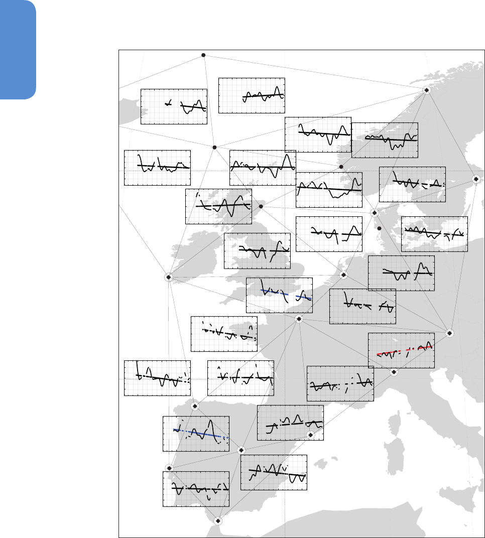
220

Chapter 2 Observations: Atmosphere and Surface

45N

Stockholm

Jan Mayen

Milan

Torshavn

Paris-Orly

Lisboa

Valentia

Aberdeen

Kremsmuenster

de Bilt

Bodo

Bergen

Vestervig

Madrid

La_corunya

Gibraltar

Barcelona

15W

-1

1900 1950 2000

-1

1900

1950

2000

-1

1900 1950 2000

-1

1900 1950 2000

-1

1900 1950 2000

-1

1900 1950 2000

-1

1900 1950 2000

-1

1900 1950 2000

-1

1900 1950 2000

-1

1900 1950 2000

-1

1900 1950 2000

-1

1900 1950 2000

-1

1900 1950 2000

-1

1900 1950 2000

-1

1900 1950 2000

-1

1900 1950 2000

-1

1900 1950 2000

-1

1900 1950 2000

-1

1900 1950 2000

-1

1900 1950 2000

-1

1900 1950 2000

-1

1900 1950 2000

-1

1900

1950 2000

-1

1900 1950

2000

Figure 2.35 | 99th percentiles of geostrophic wind speeds for winter (DJF). Triangles show regions where geostrophic wind speeds have been calculated from in situ surface pres-

sure observations. Within each pressure triangle, Gaussian low-pass ﬁltered curves and estimated linear trends of the 99th percentile of these geostrophic wind speeds for winter

are shown. The ticks of the time (horizontal) axis range from 1875 to 2005, with an interval of 10 years. Disconnections in lines show periods of missing data. Red (blue) trend lines

indicate upward (downward) signiﬁcant trends (i.e., a trend of zero lies outside the 95% conﬁdence interval). (From Wang et al., 2011.)

Studies that have examined trends in wind extremes from observa-

tions or regional reanalysis products tend to point to declining trends

in extremes in mid-latitudes (Pirazzoli and Tomasin, 2003; Smits et al.,

2005; Pryor et al., 2007; Zhang et al., 2007b) and increasing trends

in high latitudes (Lynch et al., 2004; Turner et al., 2005; Hundecha et

al., 2008; Stegall and Zhang, 2012). Other studies have compared the

trends from observations with reanalysis data and reported differing

or even opposite trends in the reanalysis products (Smits et al., 2005;

McVicar et al., 2008). On the other hand, declining trends reported

by Xu et al. (2006b) over China between 1969 and 2000 were gener-

ally consistent with trends in NCEP reanalysis. Trends extracted from

reanalysis products must be treated with caution however, although

usually with later generation products providing improvements over

older products (Box 2.3).

In summary, conﬁdence in large scale changes in the intensity of

extreme extratropical cyclones since 1900 is low. There is also low con-

ﬁdence for a clear trend in storminess proxies over the last century

due to inconsistencies between studies or lack of long-term data in

some parts of the world (particularly in the SH). Likewise, conﬁdence in

trends in extreme winds is low, owing to quality and consistency issues

with analysed data.

221

Observations: Atmosphere and Surface Chapter 2

Box 2.4 | Extremes Indices

As SREX highlighted, there is no unique deﬁnition of what constitutes a climate extreme in the scientiﬁc literature given variations in

regions and sectors affected (Stephenson et al., 2008). Much of the available research is based on the use of so-called ‘extremes indices’

(Zhang et al., 2011). These indices can either be based on the probability of occurrence of given quantities or on absolute or percentage

threshold exceedances (relative to a ﬁxed climatological period) but also include more complex deﬁnitions related to duration, intensity

and persistence of extreme events. For example, the term ‘heat wave’ can mean very different things depending on the index formula-

tion for the application for which it is required (Perkins and Alexander, 2012).

Box 2.4, Table 1 lists a number of speciﬁc indices that appear widely in the literature and have been chosen to provide some consistency

across multiple chapters in AR5 (along with the location of associated ﬁgures and text). These indices have been generally chosen for

their robust statistical properties and their applicability across a wide range of climates. Another important criterion is that data for

these indices are broadly available over both space and time. The existing near-global land-based data sets cover at least the post-1950

period but for regions such as Europe, North America, parts of Asia and Australia much longer analyses are available. The same indices

used in observational studies (this chapter) are also used to diagnose climate model output (Chapters 9, 10, 11 and 12).

The types of indices discussed here do not include indices such as NIÑO3 representing positive and negative phases of ENSO (Box 2.5),

nor do they include extremes such as 1 in 100 year events. Typically extreme indices assessed here reﬂect more ‘moderate’ extremes,

for example, events occurring as often as 5% or 10% of the time (Box 2.4, Table 1). Predeﬁned extreme indices are usually easier to

obtain than the underlying daily climate data, which are not always freely exchanged by meteorological services. However, some of

these indices do represent rarer events, for example, annual maxima or minima. Analyses of these and rarer extremes (e.g., with longer

Box 2.4, Table 1 | Deﬁnitions of extreme temperature and precipitation indices used in IPCC (after Zhang et al., 2011). The most common units are shown but these

may be shown as normalized or relative depending on application in different chapters.

Index Descriptive name Deﬁnition Units Figures/Tables Section

TXx Warmest daily Tmax Seasonal/annual maximum value of daily maximum

temperature

ºC Box 2.4, Figure 1, Figures 9.37,

10.17, 12.13

Box 2.4, 9.5.4.1, 10.6.1.1,

12.4.3.3

TNx Warmest daily Tmin Seasonal/annual maximum value of daily minimum

temperature

ºC Figures 9.37, 10.17 9.5.4.1, 10.6.1.1

TXn Coldest daily Tmax Seasonal/annual minimum value of daily maximum

temperature

ºC Figures 9.37, 10.17, 12.13 9.5.4.1, 10.6.1.1, 12.4.3.3

TNn Coldest daily Tmin Seasonal/annual minimum value of daily minimum

temperature

ºC Figures 9.37, 10.17, 12.13 9.5.4.1, 10.6.1.1

TN10p Cold nights Days (or fraction of time) when daily minimum

temperature <10th percentile

Days (%) Figures 2.32, 9.37, 10.17

Tables 2.11, 2.12

2.6.1, 9.5.4.1, 10.6.1.1,

11.3.2.5.1

TX10p Cold days Days (or fraction of time) when daily maximum

temperature <10th percentile

Days (%) Figures 2.32, 9.37, 10.17, 11.17 2.6.1, 9.5.4.1, 10.6.1.1,

11.3.2.5.1,

TN90p Warm nights Days (or fraction of time) when daily minimum

temperature >90th percentile

Days (%) Figures 2.32, 9.37, 10.17

Tables 2.11, 2.12

2.6.1, 9.5.4.1, 10.6.1.1,

11.3.2.5.1

TX90p Warm days Days (or fraction of time) when daily maximum

temperature >90th percentile

Days (%) Figures 2.32, 9.37, 10.17, 11.17

Tables 2.11, 2.12

2.6.1, 9.5.4.1, 10.6.1.1,

11.3.2.5.1,

FD Frost days Frequency of daily minimum temperature <0°C Days Figures 9.37, 12.13

Table 2.12

2.6.1, 9.5.4.1, 10.6.1.1,

12.4.3.3

TR Tropical nights Frequency of daily minimum temperature >20°C Days Figures 9.37, 12.13 9.5.4.1, 12.4.3.3

RX1day Wettest day Maximum 1-day precipitation mm Figures 9.37, 10.10

Table 2.12, 12.27

2.6.2.1, 9.5.4.1, 10.6.1.2,

12.4.5.5

RX5day Wettest consecutive ﬁve days Maximum of consecutive 5-day precipitation mm Figures 9.37, 12.26, 14.1 9.5.4.1, 10.6.1.2, 12.4.5.5,

14.2.1

SDII Simple daily intensity index Ratio of annual total precipitation to the number of

wet days (≥1 mm)

mm day

–1

Figures 2.33, 9.37, 14.1 2.6.2.1, 9.5.4.1, 14.2.1

R95p Precipitation from very wet

days

Amount of precipitation from days >95th percentile mm Figures 2.33, 9.37, 11.17

Table 2.12

2.6.2.1, 9.5.4.1, 11.3.2.5.1

CDD Consecutive dry days Maximum number of consecutive days when

precipitation <1 mm

Days Figures 2.33, 9.37, 12.26, 14.1 2.6.2.3, 9.5.4.1, 12.4.5.5,

14.2.1

(continued on next page)

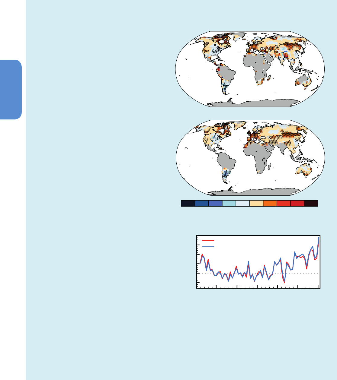
222

Chapter 2 Observations: Atmosphere and Surface

return period thresholds) are making their way into a

growing body of literature which, for example, are using

Extreme Value Theory (Coles, 2001) to study climate

extremes (Zwiers and Kharin, 1998; Brown et al., 2008;

Sillmann et al., 2011; Zhang et al., 2011; Kharin et al.,

2013).

Extreme indices are more generally deﬁned for daily

temperature and precipitation characteristics (Zhang

et al., 2011) although research is developing on the

analysis of sub-daily events but mostly only on regional

scales (Sen Roy, 2009; Shiu et al., 2009; Jones et al.,

2010; Jakob et al., 2011; Lenderink et al., 2011; Shaw

et al., 2011). Temperature and precipitation indices

are sometimes combined to investigate ‘extremeness’

(e.g., hydroclimatic intensity, HY-INT; Giorgi et al., 2011)

and/or the areal extent of extremes (e.g., the Climate

Extremes Index (CEI) and its variants (Gleason et al.,

2008; Gallant and Karoly, 2010; Ren et al., 2011). Indi-

ces rarely include other weather and climate variables,

such as wind speed, humidity or physical impacts (e.g.,

streamﬂow) and phenomena. Some examples are avail-

able in the literature for wind-based (Della-Marta et al.,

2009) and pressure-based (Beniston, 2009) indices, for

health-relevant indices combining temperature and rel-

ative humidity characteristics (Diffenbaugh et al., 2007;

Fischer and Schär, 2010) and for a range of dryness or

drought indices (e.g., Palmer Drought Severity Index

(PDSI) Palmer, 1965; Standardised Precipitation Index

(SPI), Standardised Precipitation Evapotranspiration

Index (SPEI) Vicente-Serrano et al., 2010) and wetness

indices (e.g., Standardized Soil Wetness Index (SSWI);

Vidal et al., 2010). (continued on next page)

In addition to the complication of deﬁning an index,

the results depend also on the way in which indices

are calculated (to create global averages, for example).

This is due to the fact that different algorithms may be

employed to create grid box averages from station data,

or that extremes indices may be calculated from grid-

ded daily data or at station locations and then gridded.

All of these factors add uncertainty to the calculation of

an extreme. For example, the spatial patterns of trends

in the hottest day of the year differ slightly between

data sets, although when globally averaged, trends are

similar over the second half of the 20th century (Box

2.4, Figure 1). Further discussion of the parametric and

structural uncertainties in data sets is given in Box 2.1.

Box 2.4 (continued)

Box 2.4, Figure 1 | Trends in the warmest day of the year using different data sets for

the period 1951–2010. The data sets are (a) HadEX2 (Donat et al., 2013c) updated to

include the latest version of the European Climate Assessment data set (Klok and Tank,

2009), (b) HadGHCND (Caesar et al., 2006) using data updated to 2010 (Donat et al.,

2013a) and (c) Globally averaged annual warmest day anomalies for each data set.

Trends were calculated only for grid boxes that had at least 40 years of data during this

period and where data ended no earlier than 2003. Grey areas indicate incomplete or

missing data. Black plus signs (+) indicate grid boxes where trends are signiﬁcant (i.e., a

trend of zero lies outside the 90% conﬁdence interval). Anomalies are calculated using

grid boxes only where both data sets have data and where 90% of data are available.

(a) HadEX2 1951-2010

(b) HadGHCND 1951-2010

Trend (°C per decade)

2.0

1.5

1.0

0.5

0.0

-0.5

1950

-1 -0.75 -0.5 -0.25 0 0.25 0.5 0.75 1

1960 1970 1980 1990 2000

HadEX2

HadGHCND

2010

Temperature anomaly (ºC)

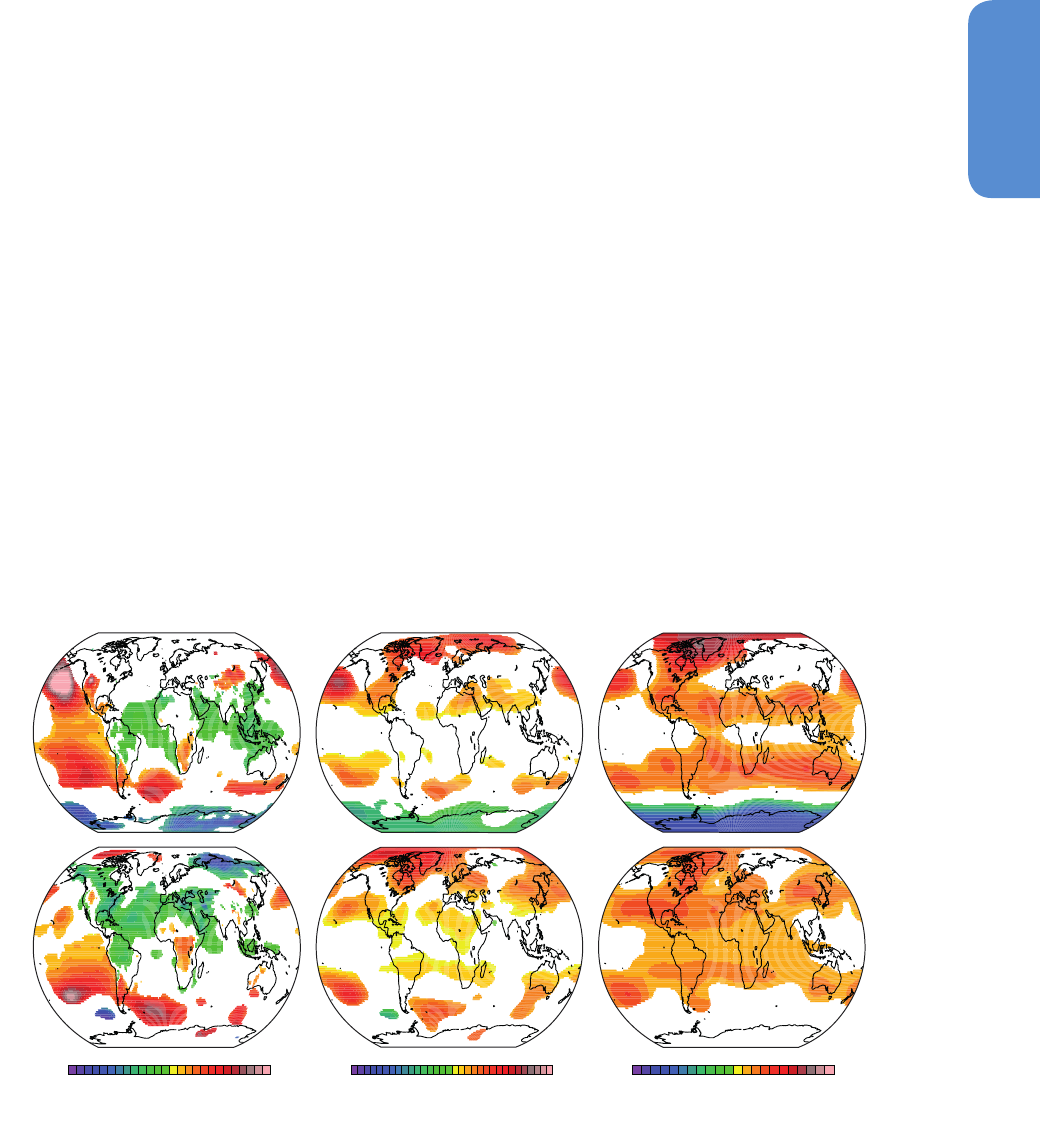
223

Observations: Atmosphere and Surface Chapter 2

2.7 Changes in Atmospheric Circulation and

Patterns of Variability

Changes in atmospheric circulation and indices of climate variability, as

expressed in sea level pressure (SLP), wind, geopotential height (GPH),

and other variables were assessed in AR4. Substantial multi-decadal

variability was reported in the large-scale atmospheric circulation over

the Atlantic and the Paciﬁc. With respect to trends, a decrease was

found in tropospheric GPH over high latitudes of both hemispheres

and an increase over the mid-latitudes in boreal winter for the period

1979–2001. These changes were found to be associated with an inten-

siﬁcation and poleward displacement of Atlantic and southern mid-lat-

itude jet streams and enhanced storm track activity in the NH from the

1960s to at least the 1990s. Changes in the North Atlantic Oscillation

(NAO) and the Southern Annular Mode (SAM) towards their positive

phases were observed, but it was noted that the NAO returned to its

long-term mean state from the mid-1990s to the early 2000s.

Since AR4, more and improved observational data sets and reanalysis

data sets (Box 2.3) have been published. Uncertainties and inaccuracies

in all data sets are better understood (Box 2.1). The studies since AR4

assessed in this section support the poleward movement of circulation

features since the 1970s and the change in the SAM. At the same time,

large decadal-to-multidecadal variability in atmospheric circulation is

found that partially offsets previous trends in other circulation features

such as the NAO or the Paciﬁc Walker circulation.

This section assesses observational evidence for changes in atmos-

pheric circulation in ﬁelds of SLP, GPH, and wind, in circulation features

(such as the Hadley and Walker circulation, monsoons, or jet streams;

Annex III: Glossary), as well as in circulation variability modes. Regional

climate effects of the circulation changes are discussed in Chapter 14.

2.7.1 Sea Level Pressure

AR4 concluded that SLP in December to February decreased between

1948 and 2005 in the Arctic, Antarctic and North Paciﬁc. More recent

studies using updated data for the period 1949–2009 (Gillett and Stott,

2009) also ﬁnd decreases in SLP in the high latitudes of both hemi-

spheres in all seasons and increasing SLP in the tropics and subtropics

most of the year. However, due to decadal variability SLP trends are

sensitive to the choice of the time period (Box 2.2), and they depend

on the data set.

The spatial distribution of SLP represents the distribution of atmos-

pheric mass, which is the surface imprint of the atmospheric circula-

tion. Barometric measurements are made in weather stations or on

board ships. Fields are produced from the observations by interpolation

or using data assimilation into weather models. One of the most widely

used observational data sets is HadSLP2 (Allan and Ansell, 2006),

which integrates 2228 historical global terrestrial stations with marine

observations from the ICOADS on a 5° × 5°grid. Other observation

products (e.g., Trenberth and Paolino, 1980; for the extratropical NH)

or reanalyses are also widely used to address changes in SLP. Although

the quality of SLP data is considered good, there are discrepancies

between gridded SLP data sets in regions with sparse observations,

e.g., over Antarctica (Jones and Lister, 2007).

Van Haren et al. (2012) found a strong SLP decrease over the Mediter-

ranean in January to March from 1961 to 2000. For the more recent

period (1979–2012) trends in SLP, consistent across different data sets

(shown in Figure 2.36 for ERA-Interim), are negative in the tropical

and northern subtropical Atlantic during most of the year as well as,

in May to October, in northern Siberia. Positive trends are found year-

round over the North and South Paciﬁc and South Atlantic. Trends in

Trend (hPa per decade)

-1.2 -0.6 0 0.6 1.2

Trend (gpm per decade)

-30 -15 015 30

-40 -20 02040

Trend (gpm per decade)

Sea-level pressure 500hPa geopotential height 100hPa geopotential height

Nov-AprMay-Oct

Figure 2.36 | Trends in (left) sea level pressure (SLP), (middle) 500 hPa geopotential height (GPH) and (right) 100 hPa GPH in (top) November to April 1979/1980 to 2011/2012

and (bottom) May to October 1979 to 2011 from ERA-Interim data. Trends are shown only if signiﬁcant (i.e., a trend of zero lies outside the 90% conﬁdence interval).

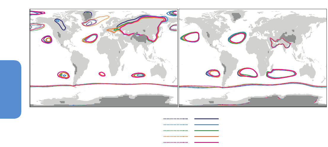
224

Chapter 2 Observations: Atmosphere and Surface

the equatorial Paciﬁc zonal SLP gradient during the 20th century (e.g.,

Vecchi et al., 2006; Power and Kociuba, 2011a, 2011b) are discussed

in Section 2.7.5.

The position and strength of semi-permanent pressure centres show

no clear evidence for trends since 1951. However, prominent variability

is found on decadal time scales (Figure 2.37). Consistent across differ-

ent data sets, the Azores high and the Icelandic low in boreal winter,

as captured by the high and low SLP contours, were both small in the

1960s and 1970s, large in the 1980s and 1990s, and again smaller in

the 2000s. Favre and Gershunov (2006) ﬁnd an eastward shift of the

Aleutian low from the mid-1970s to 2001, which persisted during the

2000s (Figure 2.37). The Siberian High exhibits pronounced decad-

al-to-multidecadal variability (Panagiotopoulos et al., 2005; Huang et

al., 2010), with a recent (1998 to 2012) strengthening and northwest-

ward expansion (Zhang et al., 2012b). In boreal summer, the Atlantic and

Paciﬁc high-pressure systems extended more westward in the 1960s

and 1970s than later. On interannual time scales, variations in pressure

centres are related to modes of climate variability. Trends in the indices

that capture the strength of these modes are reported in Section 2.7.8,

their characteristics and impacts are discussed in Chapter 14.

In summary, sea level pressure has likely decreased from 1979 to 2012

over the tropical Atlantic and increased over large regions of the Paciﬁc

and South Atlantic, but trends are sensitive to the time period analysed

owing to large decadal variability.

2.7.2 Surface Wind Speed

AR4 concluded that mid-latitude westerly winds have general-

ly increased in both hemispheres. Because of shortcomings in the

observations, SREX stated that conﬁdence in surface wind trends is

low. Further studies assessed here conﬁrm this assessment.

1004 hPa 1020.5 hPa

November-April

May-October

1961-1970

1971-1980

1981-1990

1991-2000

2001-2010

Figure 2.37 | Decadal averages of sea level pressure (SLP) from the 20th Century Reanalysis (20CR) for (left) November of previous year to April and (right) May to October shown

by two selected contours: 1004 hPa (dashed lines) and 1020.5 hPa (solid lines). Topography above 2 km above mean sea level in 20CR is shaded in dark grey.

Surface wind measurements over land and ocean are based on largely

separate observing systems. Early marine observations were based on

ship speed through the water or sails carried or on visual estimates

of sea state converted to the wind speed using the Beaufort scale.

Anemometer measurements were introduced starting in the 1950s.

The transition from Beaufort to measured winds introduced a spurious

trend, compounded by an increase in mean anemometer height over

time (Kent et al., 2007; Thomas et al., 2008). ICOADS release 2.5 (Wood-

ruff et al., 2011) contains information on measurement methods and

wind measurement heights, permitting adjustment for these effects.

The ICOADS-based data set WASWind (1950–2010; Tokinaga and Xie,

2011a) and the interpolated product NOCS v.2.0 (1973–present; Berry

and Kent, 2011) include such corrections, among other improvements.

Marine surface winds are also measured from space using various

microwave range instruments: scatterometers and synthetic aper-

ture radars retrieve wind vectors, while altimeters and passive radi-

ometers measure wind speed only (Bourassa et al., 2010). The latter

type provides the longest continuous record, starting in July 1987.

Satellite-based interpolated marine surface wind data sets use objec-

tive analysis methods to blend together data from different satellites

and atmospheric reanalyses. The latter provide wind directions as in

Blended Sea Winds (BSW; Zhang et al., 2006), or background ﬁelds

as in Cross-Calibrated Multi-Platform winds (CCMP; Atlas et al., 2011)

and OAFlux (Yu and Weller, 2007). CCMP uses additional dynamical

constraints, in situ data and a recently homogenized data set of SSM/I

observations (Wentz et al., 2007), among other satellite sources.

Figure 2.38 compares 1988–2010 linear trends in surface wind speeds

from interpolated data sets based on satellite data, from interpolat-

ed and non-interpolated data sets based on in situ data, and from

atmospheric reanalyses. Note that these trends over a 23-year-long

period primarily reﬂect decadal variability in winds, rather than long-

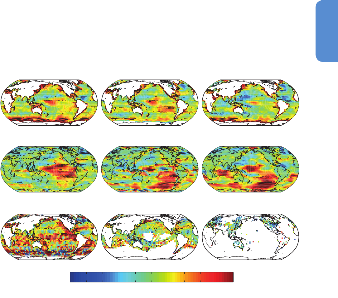
225

Observations: Atmosphere and Surface Chapter 2

term climate change (Box 2.2). Kent et al. (2012) recently intercom-

pared several of these data sets and found large differences. The differ-

ences in trend patterns in Figure 2.38 are large as well. Nevertheless,

some statistically signiﬁcant features are present in most data sets,

including a pattern of positive and negative trend bands across the

North Atlantic Ocean (Section 2.7.6.2.) and positive trends along the

west coast of North America. Strengthening of the Southern Ocean

winds, consistent with the increasing trend in the SAM (Section 2.7.8)

and with the observed changes in wind stress ﬁelds described in Sec-

tion 3.4.4, can be seen in satellite-based analyses and atmospheric

reanalyses in Figure 2.38. Alternating Southern Ocean trend signs in

the NOCS v.2.0 panel are due to interpolation of very sparse in situ

data (cf. the panel for the uninterpolated WASWind product).

Surface winds over land have been measured with anemometers on a

global scale for decades, but until recently the data have been rarely

used for trend analysis. Global data sets lack important meta informa-

tion on instrumentation and siting (McVicar et al., 2012). Long, homog-

enized instrumental records are rare (e.g., Usbeck et al., 2010; Wan et

al., 2010). Moreover, wind speed trends are sensitive to the anemome-

ter height (Troccoli et al., 2012). Winds near the surface can be derived

from reanalysis products (Box 2.3), but discrepancies are found when

comparing trends therein with trends for land stations (Smits et al.,

2005; McVicar et al., 2008).

Over land, a weakening of seasonal and annual mean as well as max-

imum winds is reported for many regions from around the 1960s or

1970s to the early 2000s (a detailed review is given in McVicar et al.

(2012)), including China and the Tibetan Plateau (Xu et al., 2006b; Guo

et al., 2010) (but levelling off since 2000; Lin et al., 2012), Western and

southern Europe (e.g., Earl et al., 2013), much of the USA (Pryor et

al., 2007), Australia (McVicar et al., 2008) and southern and western

(a) CCMP (b) OAFlux (c) BSW

(d) ERA−Interim (e) NNR (f) 20CR

(g) NOCS v2.0 (h) WASWind (i) Surface winds on the land

Trend (m s

-1

per decade)

−0.5 −0.4 −0.3 −0.2 −0.1 0 0.1 0.2 0.3 0.4 0.5

Figure 2.38 | Trends in surface wind speed for 1988–2010. Shown in the top row are data sets based on the satellite wind observations: (a) Cross-Calibrated Multi-Platform wind

product (CCMP; Atlas et al., 2011); (b) wind speed from the Objectively Analyzed Air-Sea Heat Fluxes data set, release 3 (OAFlux); (c) Blended Sea Winds (BSW; Zhang et al., 2006); in

the middle row are data sets based on surface observations: (d) ERA-Interim; (e) NCEP-NCAR, v.1 (NNR); (f) 20th Century Reanalysis (20CR, Compo et al., 2011), and in the bottom

row are surface wind speeds from atmospheric reanalyses: (g) wind speed from the Surface Flux Data set, v.2, from NOC, Southampton, UK (Berry and Kent, 2009); (h) Wave- and

Anemometer-based Sea Surface Wind (WASWind; Tokinaga and Xie, 2011a)); and (i) Surface Winds on the Land (Vautard et al., 2010). Wind speeds correspond to 10 m heights

in all products. Land station winds (panel f) are also for 10 m (but anemometer height is not always reported) except for the Australian data where they correspond to 2 m height.

To improve readability of plots, all data sets (including land station data) were averaged to the 4° × 4° uniform longitude-latitude grid. Trends were computed for the annually

averaged timeseries of 4° × 4° cells. For all data sets except land station data, an annual mean was considered available only if monthly means for no less than eight months were

available in that calendar year. Trend values were computed only if no less than 17 years had values and at least 1 year was available among the ﬁrst and last 3 years of the period.

White areas indicate incomplete or missing data. Black plus signs (+) indicate grid boxes where trends are signiﬁcant (i.e., a trend of zero lies outside the 90% conﬁdence interval).

226

Chapter 2 Observations: Atmosphere and Surface

Canada (Wan et al., 2010). Increasing wind speeds were found at high

latitudes in both hemispheres, namely in Alaska from 1921 to 2001

(Lynch et al., 2004), in the central Canadian Arctic and Yukon from the

1950 to the 2000s (Wan et al., 2010) and in coastal Antarctica over the

second half of the 20th century (Turner et al., 2005). A global review

of 148 studies showed that near-surface terrestrial wind speeds are

declining in the Tropics and the mid-latitudes of both hemispheres at

a rate of −0.14 m s

−1

per decade (McVicar et al., 2012). Vautard et al.

(2010), analysing a global land surface wind data set from 1979 to

2008, found negative trends on the order of –0.1 m s

–1

per decade

over large portions of NH land areas. The wind speed trend pattern

over land inferred from their data (1988–2010, Figure 2.38) has many

points with magnitudes much larger than those in the reanalysis prod-

ucts, which appear to underestimate systematically the wind speed

over land, as well as in coastal regions (Kent et al., 2012).

In summary, conﬁdence is low in changes in surface wind speed over

the land and over the oceans owing to remaining uncertainties in data

sets and measures used.

2.7.3 Upper-Air Winds

In contrast to surface winds, winds above the planetary bounda-

ry layer have received little attention in AR4. Radiosondes and pilot

balloon observations are available from around the 1930s (Stickler et

al., 2010). Temporal inhomogeneities in radiosonde wind records are

less common, but also less studied, than those in radiosonde temper-

ature records (Gruber and Haimberger, 2008; Section 2.4.4.3). Upper

air winds can also be derived from tracking clouds or water vapour

in satellite imagery (Menzel, 2001) or from measurements using wind

proﬁlers, aircraft or thermal observations, all of which serve as an input

to reanalyses (Box 2.3).

In the past few years, interest in an accurate depiction of upper air

winds has grown, as they are essential for estimating the state and

changes of the general atmospheric circulation and for explaining

changes in the surface winds (Vautard et al., 2010). Allen and Sher-

wood (2008), analysing wind shear from radiosonde data, found sig-

niﬁcant positive zonal mean zonal wind trends in the northern extrat-

ropics in the upper troposphere and stratosphere and negative trends

in the tropical upper troposphere for the period 1979–2005. Vautard

et al. (2010) ﬁnd increasing wind speed in radiosonde observations

in the lower and middle troposphere from 1979 to 2008 over Europe

and North America and decreasing wind speeds over Central and East

Asia. However, systematic global trend analyses of radiosonde winds

are rare, prohibiting an assessment of upper-air wind trends (speciﬁc

features such as monsoons, jet streams and storms are discussed in

Sections 2.7.5, 2.7.6 and 2.6, respectively).

In summary, upper-air winds are less studied than other aspects of the

circulation, and less is known about the quality of data products, hence

conﬁdence in upper-air wind trends is low.

2.7.4 Tropospheric Geopotential Height and Tropopause

AR4 concluded that over the NH between 1960 and 2000, boreal

winter and annual means of tropospheric GPH decreased over high

latitudes and increased over the mid-latitudes. AR4 also reported an

increase in tropical tropopause height and a slight cooling of the trop-

ical cold-point tropopause.

Changes in GPH, which can be addressed using radiosonde data or

reanalysis data (Box 2.3), reﬂect SLP and temperature changes in the

atmospheric levels below. The spatial gradients of the trend indicate

changes in the upper-level circulation. As for SLP, tropopsheric GPH

trends strongly depend on the period analysed due to pronounced dec-

adal variability. For the 1979–2012 period, trends for 500 hPa GPH

from the ERA-Interim reanalysis (Figure 2.36) as well as for other rea-

nalyses show a signiﬁcant decrease only at southern high latitudes in

November to April, but signiﬁcant positive GPH trends in the subtrop-

ics and northern high latitudes. Hence the change in the time period

leads to a different trend pattern as compared to AR4. The seasonality

and spatial dependence of 500 hPa GPH trends over Antarctica was

highlighted by Neff et al. (2008), based upon radiosonde data over the

period 1957–2007.

Minimum temperatures near the tropical tropopause (and therefore

tropical tropopause height) are important as they affect the water

vapour input into the stratosphere (Section 2.2.2.1). Studies since AR4

conﬁrm the increase in tropopause height (Wang et al., 2012c). For

tropical tropopause temperatures, studies based on radiosonde data

and reanalyses partly support a cooling between the 1990s and the

early 2000s (Randel et al., 2006; Randel and Jensen, 2013), but uncer-

tainties in long-term trends of the tropical cold-point tropopause tem-

perature from radiosondes (Wang et al., 2012c; Randel and Jensen,

2013) and reanalyses (Gettelman et al., 2010) are large and conﬁdence

is therefore low.

In summary, tropospheric geopotential height likely decreased from

1979 to 2012 at SH high latitudes in austral summer and increased

in the subtropics and NH high latitudes. Conﬁdence in trends of the

tropical cold-point tropopause is low owing to remaining uncertainties

in the data.

2.7.5 Tropical Circulation

In AR4, large interannual variability of the Hadley and Walker circula-

tion was highlighted, as well as the difﬁculty in addressing changes in

these features in the light of discrepancies between data sets. AR4 also

found that rainfall in many monsoon systems exhibits decadal chang-

es, but that data uncertainties restrict conﬁdence in trends. SREX also

attributed low conﬁdence to observed trends in monsoons.

Observational evidence for trends and variability in the strength of the

Hadley and Walker circulations (Annex III: Glossary), the monsoons, and

the width of the tropical belt is based on radiosonde and

reanalyses

data (Box 2.3). In addition, changes in the tropical circulation imprint

on other ﬁelds that are observed from space (e.g., total ozone, outgo-

ing longwave radiation). Changes in the average state of the tropical

circulation are constrained to some extent by changes in the water

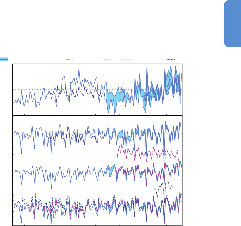
227

Observations: Atmosphere and Surface Chapter 2

cycle (Held and Soden, 2006; Schneider et al., 2010). Changes in the

monsoon systems are expressed through altered circulation, moisture

transport and convergence, and precipitation. Only a few monsoon

studies address circulation changes, while most work focuses on pre-

cipitation.

Several studies report a weakening of the global monsoon circulations

as well as a decrease of global land monsoon rainfall or of the number

of precipitation days over the past 40 to 50 years (Zhou et al., 2008,

see also SREX; Liu et al., 2011). Concerning the East Asian Monsoon,

a year-round decrease is reported for wind speeds over China at the

surface and in the lower troposphere based on surface observations

and radiosonde data (Guo et al., 2010; Jiang et al., 2010; Vautard et

al., 2010; Xu et al., 2010). The changes in wind speed are concomi-

tant with changes in pressure centres such as a westward extension

of the Western Paciﬁc Subtropical High (Gong and Ho, 2002; Zhou et

al., 2009b). A weakening of the East Asian summer monsoon since the

1920s is also found in SLP gradients (Zhou et al., 2009a). However,

trends derived from wind observations and circulation trends from

reanalysis data carry large uncertainties (Figure 2.38), and monsoon

rainfall trends depend, for example, on the deﬁnition of the monsoon

area (Hsu et al., 2011). For instance, using a new deﬁnition of monsoon

area, an increase in northern hemispheric and global summer monsoon

(land and ocean) precipitation is reported from 1979 to 2008 (Hsu et

al., 2011; Wang et al., 2012a).

The additional data sets that became available since AR4 conﬁrm the

large interannual variability of the Hadley and Walker circulation. The

strength of the northern Hadley circulation (Figure 2.39) in boreal

winter and of the Paciﬁc Walker circulation in boreal fall and winter is

largely related to the ENSO (Box 2.5). This association dominates inter-

annual variability and affects trends. Data sets do not agree well with

respect to trends in the Hadley circulation (Figure 2.39). Two widely

used reanalysis data sets, NNR and ERA-40, both have demonstrated

Hadley Circulation indices

Pacific Walker circulation indices

1880 1900 1920 1940 1960 1980 2000

-2

-4

-2

-1

-2

0.04

0.02

-0.02

-0.04

-0.06

Reanalyses (individual and spread) Reconstructions SSMI ICOADS/WASWIND HADSPL2

max

(10

kg s

-1

)

∆ω (Pa s

-1

) ∆SLP (hPa)

-0.5

0.0

0.5

∆c (octas)

-0.6

-0.4

-0.2

0.0

(m s

-1

)

u (m s

-1

)

(a)

(b)

Figure 2.39 | (a) Indices of the strength of the northern Hadley circulation in December to March (Ψ

max

is the maximum of the meridional mass stream function at 500 hPa

between the equator and 40°N). (b) Indices of the strength of the Paciﬁc Walker circulation in September to January (Δω is the difference in the vertical velocity between [10°S

to 10°N, 180°W to 100°W] and [10°S to 10°N, 100°E to 150°E] as in Oort and Yienger (1996), Δc is the difference in cloud cover between [6°N to 12°S, 165°E to 149°W] and

[18°N to 6°N, 165°E to 149°W] as in Deser et al. (2010a), v

is the effective wind index from SSM/I satellite data, updated from Sohn and Park (2010), u is the zonal wind at 10

m averaged in the region [10°S to 10°N, 160°E to 160°W], ΔSLP is the SLP difference between [5°S to 5°N, 160°W to 80°W] and [5°S to 5°N, 80°E to 160°E] as in Vecchi et

al. (2006)). Reanalysis data sets include 20CR, NCEP/NCAR, ERA-Interim, JRA-25, MERRA, and CFSR, except for the zonal wind at 10 m (20CR, NCEP/NCAR, ERA-Interim), where

available until January 2013. ERA-40 and NCEP2 are not shown as they are outliers with respect to the strength trend of the northern Hadley circulation (Mitas and Clement, 2005;

Song and Zhang, 2007; Hu et al., 2011; Stachnik and Schumacher, 2011). Observation data sets include HadSLP2 (Section 2.7.1), ICOADS (Section 2.7.2; only 1957–2009 data

are shown) and WASWIND (Section 2.7.2), reconstructions are from Brönnimann et al. (2009). Where more than one time series was available, anomalies from the 1980/1981 to

2009/2010 mean values of each series are shown.

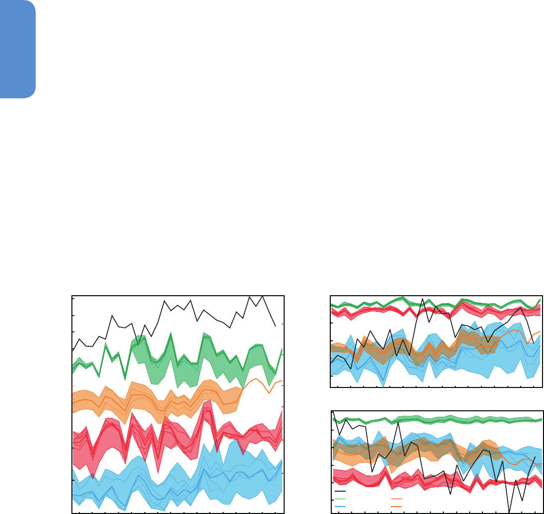
228

Chapter 2 Observations: Atmosphere and Surface

shortcomings with respect to tropical circulation; hence their increases

in the Hadley circulation strength since the 1970s might be artiﬁcial

(Mitas and Clement, 2005; Song and Zhang, 2007; Hu et al., 2011;

Stachnik and Schumacher, 2011). Later generation reanalysis data sets

including ERA-Interim (Brönnimann et al., 2009; Nguyen et al., 2013)

as well as satellite humidity data (Sohn and Park, 2010) also suggest

a strengthening from the mid 1970s to present, but the magnitude is

strongly data set dependent.

Consistent changes in different observed variables suggest a weaken-

ing of the Paciﬁc Walker circulation during much of the 20th century

that has been largely offset by a recent strengthening. A weakening

is indicated by trends in the zonal SLP gradient across the equato-

rial Paciﬁc (Section 2.7.1, Table 2.14) from 1861 to 1992 (Vecchi et

al., 2006), or from 1901 to 2004 (Power and Kociuba, 2011b). Boreal

spring and summer contribute most strongly to the centennial trend

(Nicholls, 2008; Karnauskas et al., 2009), as well as to the trend in the

second half of the 20th century (Tokinaga et al., 2012). For boreal fall

and winter, when the circulation is strongest, no trend is found in the

Paciﬁc Walker circulation based on the vertical velocity at 500 hPa from

reanalyses (Compo et al., 2011), equatorial Paciﬁc 10 m zonal winds, or

SLP in Darwin (Nicholls, 2008; Figure 2.39). However, there are incon-

sistencies between ERA-40 and NNR (Chen et al., 2008). Deser et al.

(2010a) ﬁnd changes in marine air temperature and cloud cover over

the Paciﬁc that are consistent with a weakening of the Walker circu-

lation during most of the 20th century (Section 2.5.7.1 and Yu and

Zwiers, 2010). Tokinaga et al. (2012) ﬁnd robust evidence for a weak-

ening of the Walker circulation (most notably over the Indian Ocean)

from 1950 to 2008 based on observations of cloud cover, surface wind,

and SLP. Since the 1980s or 1990s, however, trends in the Paciﬁc Walker

Tropical belt width

1980 1990 2000 2010 1980 1990 2000 2010

1980 1990 2000 2010

-30

-34

-38

Northern Hemisphere

Tropical edge latitude (°N)

Tropical edge latitude (°S)

Total tropical width (°lat)

Southern Hemisphere

Ozone

Jet Stream

Hadley Cell

Tropopause

Outgoing Longwave Radiation

circulation have reversed (Figure 2.39; Luo et al., 2012). This is evident

from changes in SLP (see equatorial Southern Oscillation Index (SOI)

trends in Table 2.14 and Box 2.5, Figure 1), vertical velocity (Compo et

al., 2011), water vapour ﬂux from satellite and reanalysis data (Sohn

and Park, 2010), or sea level height (Merriﬁeld, 2011). It is also con-

sistent with the SST trend pattern since 1979 (Meng et al., 2012; see

also Figure 2.22).

Observed changes in several atmospheric parameters suggest that the

width of the tropical belt has increased at least since 1979 (Seidel et

al., 2008; Forster et al., 2011; Hu et al., 2011). Since AR4, wind, tem-

perature, radiation, and ozone information from radiosondes, satellites,

and reanalyses had been used to diagnose the tropical belt width and

estimate their trends. Annual mean time series of the tropical belt

width from various sources are shown in Figure 2.40.

Since 1979 the region of low column ozone values typical of the tropics

has expanded in the NH (Hudson et al., 2006; Hudson, 2012). Based on

radiosonde observations and reanalyses, the region of the high tropical

tropopause has expanded since 1979, and possibly since 1960 (Seidel

and Randel, 2007; Birner, 2010; Lucas et al., 2012), although widening

estimates from different reanalyses and using different methodologies

show a range of magnitudes (Seidel and Randel, 2007; Birner, 2010).

Several lines of evidence indicate that climate features at the edges

of the Hadley cell have also moved poleward since 1979. Subtropi-

cal jet metrics from reanalysis zonal winds (Strong and Davis, 2007,

2008; Archer and Caldeira, 2008b, 2008a) and layer-average satellite

temperatures (Fu et al., 2006; Fu and Lin, 2011) also indicate widening,

although 1979–2009 wind-based trends (Davis and Rosenlof, 2011)

Figure 2.40 | Annual average tropical belt width (left) and tropical edge latitudes in each hemisphere (right). The tropopause (red), Hadley cell (blue), and jet stream (green)

metrics are based on reanalyses (NCEP/NCAR, ERA-40, JRA25, ERA-Interim, CFSR, and MERRA, see Box 2.3); outgoing longwave radiation (orange) and ozone (black) metrics are

based on satellite measurements. The ozone metric refers to equivalent latitude (Hudson et al., 2006; Hudson, 2012). Adapted and updated from Seidel et al. (2008) using data

presented in Davis and Rosenlof (2011) and Hudson (2012). Where multiple data sets are available for a particular metric, all are shown as light solid lines, with shading showing

their range and a heavy solid line showing their median.

229

Observations: Atmosphere and Surface Chapter 2

are not statistically signiﬁcant. Changes in subtropical outgoing long-

wave radiation, a surrogate for high cloud, also suggest widening (Hu

and Fu, 2007), but the methodology and results are disputed (Davis

and Rosenlof, 2011). Widening of the tropical belt is also found in pre-

cipitation patterns (Hu and Fu, 2007; Davis and Rosenlof, 2011; Hu et

al., 2011; Kang et al., 2011; Zhou et al., 2011), including in SH regions

(Cai et al., 2012).

The qualitative consistency of these observed changes in independent

data sets suggests a widening of the tropical belt between at least

1979 and 2005 (Seidel et al., 2008), and possibly longer. Widening esti-

mates range between around 0° and 3° latitude per decade, but their

uncertainties have been only partially explored (Birner, 2010; Davis and

Rosenlof, 2011).

In summary, large interannual-to-decadal variability is found in the

strength of the Hadley and Walker circulation. The conﬁdence in trends

in the strength of the Hadley circulation is low due to uncertainties in

reanalysis data sets. Recent strengthening of the Paciﬁc Walker circu-

lation has largely offset the weakening trend from the 19th century

to the 1990s (high conﬁdence). Several lines of independent evidence

indicate a widening of the tropical belt since the 1970s. The suggested

weakening of the East Asian monsoon has low conﬁdence, given the

nature and quality of the evidence.

2.7.6 Jets, Storm Tracks and Weather Types

2.7.6.1 Mid-latitude and Subtropical Jets and Storm Track

Position

AR4 reported a poleward displacement of Atlantic and southern polar

front jet streams from the 1960s to at least the mid-1990s and a pole-

ward shift of the northern hemispheric storm tracks. However, it was

also noted that uncertainties are large and that NNR and ERA-40 dis-

agree in important aspects. SREX also reported a poleward shift of NH

and SH storm tracks. Studies since AR4 conﬁrm that in the NH, the jet

core has been migrating towards the pole since the 1970s, but trends

in the jet speed are uncertain. Additional studies assessed here further

support the poleward shift of the North Atlantic storm track from the

1950s to the early 2000s.

Subtropical and mid-latitude jet streams are three-dimensional enti-

ties that vary meridionally, zonally, and vertically. The position of the

mid-latitude jet streams is related to the position of the mid-latitude

storm tracks; regions of enhanced synoptic activity due to the pas-

sage of cyclones (Section 2.6). Jet stream winds can be determined

from radiosonde measurements of GPH using quasi-geostrophic ﬂow

assumptions. Using reanalysis data sets (Box 2.3), it is possible to track

three-dimensional jet variations by identifying a surface of maximum

wind (SMW), although a high vertical resolution is required for identi-

ﬁcation of jets.

Various new analyses based on NCEP/NCAR and ERA-40 reanalyses as

well as MSU/AMSU lower stratospheric temperatures (Section 2.4.4)

conﬁrm that the jet streams (mid-latitude and subtropical) have been

moving poleward in most regions in the NH over the last three decades

(Fu et al., 2006; Hu and Fu, 2007; Strong and Davis, 2007; Archer and

Caldeira, 2008a; Fu and Lin, 2011) but no clear trend is found in the SH

(Swart and Fyfe, 2012). There is inconsistency with respect to jet speed

trends based upon whether one uses an SMW-based or isobaric-based

approach (Strong and Davis, 2007, 2008; Archer and Caldeira, 2008b,

2008a) and the choice of analysis periods due to inhomogeneities in

reanalyses (Archer and Caldeira, 2008a). In general, jets have become

more common (and jet speeds have increased) over the western and

central Paciﬁc, eastern Canada, the North Atlantic and Europe (Strong

and Davis, 2007; Barton and Ellis, 2009), trends that are concomitant

with regional increases in GPH gradients and circumpolar vortex con-

traction (Frauenfeld and Davis, 2003; Angell, 2006). From a climate

dynamics perspective, these trends are driven by regional patterns of

tropospheric and lower stratospheric warming or cooling and thus are

coupled to large-scale circulation variability.

The North Atlantic storm track is closely associated with the NAO

(Schneidereit et al., 2007). Studies based on ERA-40 reanalysis (Schnei-

dereit et al., 2007), SLP measurements from ships (Chang, 2007), sea

level time series (Vilibic and Sepic, 2010), and cloud analyses (Bender

et al., 2012) support a poleward shift and intensiﬁcation of the North

Atlantic cyclone tracks from the 1950s to the early 2000s (Sorteberg

and Walsh, 2008; Cornes and Jones, 2011).

2.7.6.2 Weather Types and Blocking

In AR4, weather types were not assessed as such, but an increase in

blocking frequency in the Western Paciﬁc and a decrease in North

Atlantic were noted.

Changes in the frequency of weather types are of interest since weath-

er extremes are often associated with speciﬁc weather types. For

instance, persistent blocking of the westerly ﬂow was essential in the

development of the 2010 heat wave in Russia (Dole et al., 2011) (Sec-

tion 9.5.2.2 and Box 14.2). Synoptic classiﬁcations or statistical clus-

tering (Philipp et al., 2007) are commonly used to classify the weather

on a given day. Feature-based methods are also used (Croci-Maspoli

et al., 2007a). All these methods require daily SLP or upper-level ﬁelds.

Trends in synoptic weather types have been best analysed for central

Europe since the mid-20th century, where several studies describe an

increase in westerly or cyclonic weather types in winter but an increase

of anticyclonic, dry weather types in summer (Philipp et al., 2007;

Werner et al., 2008; Trnka et al., 2009). An eastward shift of blocking

events over the North Atlantic (fewer cases of blocking over Green-

land and more frequent blocking over the eartern North Atlantic) and

the North Paciﬁc was found by Davini et al. (2012) using NCEP/NCAR

reanalysis since 1951 and by Croci-Maspoli et al. (2007a) in ERA-40

reanalysis during the period 1957–2001. Mokhov et al. (2013) ﬁnd an

increase in blocking duration over the NH year-round since about 1990

in a study based on NCEP/NCAR reanalysis data from 1969–2011. For

the SH, Dong et al. (2008) found a decrease in number of blocking days

but increase in intensity of blocking over the period 1948–1999. Dif-

ferences in blocking index deﬁnitions, the sensitivity of some indices to

changes in the mean ﬁeld, and strong interannual variability in all sea-

sons (Kreienkamp et al., 2010), partly related to circulation variability

modes (Croci-Maspoli et al., 2007b), complicate a global assessment

of blocking trends.

230

Chapter 2 Observations: Atmosphere and Surface

In summary, there is evidence for a poleward shift of storm tracks and

jet streams since the 1970s. Based on the consistency of these trends

with the widening of the tropical belt (Section 2.7.5), trends that are

based on many different data sets, variables, and approaches, it is likely

that circulation features have moved poleward since the 1970s. Meth-

odological differences between studies mean there is low conﬁdence

in characterizing the global nature of any change in blocking.

2.7.7 Stratospheric Circulation

Changes in the polar vortices were assessed in AR4. A signiﬁcant

decrease in lower-stratospheric GPH in summer over Antarctica since

1969 was found, whereas trends in the Northern Polar Vortex were

considered uncertain owing to its large variability.

The most important characteristics of the stratospheric circulation for

climate and for trace gas distribution are the winter and spring polar

vortices and Sudden Stratospheric Warmings (rapid warmings of the

middle stratosphere that may lead to a collapse of the Polar Vortex),

the Quasi-Biennial Oscillation (an oscillation of equatorial zonal winds

with a downward phase propagation) and the Brewer-Dobson circu-

lation (BDC, the meridional overturning circulation transporting air

upward in the tropics, poleward to the winter hemisphere, and down-

ward at polar and subpolar latitudes; Annex III: Glossary). Radiosonde

observations, reanalysis data sets and space-borne temperature or

trace gas observations are used to address changes in the stratospher-

ic circulation, but all of these sources of information carry large trend

uncertainties.

The AR4 assessment was corroborated further in Forster et al. (2011)

and in updated 100 hPa GPH trends from ERA-Interim reanalysis (Box

2.3, Figure 2.36). There is high conﬁdence that lower stratospheric GPH

over Antarctica has decreased in spring and summer at least since

1979. Cohen et al. (2009) reported an increase in the number of Arctic

sudden stratospheric warmings during the last two decades. However,

interannual variability in the Arctic Polar Vortex is large, uncertainties in

reanalysis products are high (Tegtmeier et al., 2008), and trends depend

strongly on the time period analysed (Langematz and Kunze, 2008).

The BDC is only indirectly observable via wave activity diagnostics

(which represent the main driving mechanism of the BDC), via tem-

peratures or via the distribution of trace gases which may allow the

determination of the ‘age of air’ (i.e., the time an air parcel has resided

in the stratosphere after its entry from the troposphere). Randel et al.

(2006), found a sudden decrease in global lower stratospheric water

vapour and ozone around 2001 that is consistent with an increase in

the mean tropical upwelling, that is, the tropical branch of the BDC

(Rosenlof and Reid, 2008; Section 2.2.2.1; Lanzante, 2009; Randel and

Jensen, 2013). On the other hand, Engel et al. (2009) found no statisti-

cally signiﬁcant change in the age of air in the 24-35 km layer over the

NH mid-latitudes from measurements of chemically inert trace gases

from 1975 to 2005. However, this does not rule out trends in the lower

stratospheric branch of the BDC or trends in mid to low latitude mixing

(Bonisch et al., 2009; Ray et al., 2010). All of these methods are subject

to considerable uncertainties, and they might shed light only on some

aspects of the BDC. Conﬁdence in trends in the BDC is therefore low.

In summary, it is likely that lower-stratopheric geopotential height over

Antarctica has decreased in spring and summer at least since 1979.

Owing to uncertainties in the data and approaches used, conﬁdence in

trends in the Brewer–Dobson circulation is low.

2.7.8 Changes in Indices of Climate Variability

AR4 assessed changes in indices of climate variability. The NAO and

SAM were found to exhibit positive trends (strengthened mid-latitude

westerlies) from the 1960s to 1990s, but the NAO has returned to its

long-term mean state since then.

Indices of climate variability describe the state of the climate system

with regards to individual modes of climate variability. Together with

corresponding spatial patterns, they summarize large fractions of spa-

tio-temporal climate variability. Inferences about signiﬁcant trends in

indices are generally hampered by relative shortness of climate records,

their uncertainties and the presence of large variability on decadal and

multidecadal time scales.

Table 2.14 summarizes observed changes in well-known indices of

climate variability (see Box 2.5, Table 1 for precise deﬁnitions). Even

the indices that explicitly include detrending of the entire record (e.g.,

Deser et al., 2010b), can exhibit statistically signiﬁcant trends over

shorter sub-periods. Conﬁdence intervals in Table 2.14 that do not con-

tain zero indicate trend signiﬁcance at 10% level; however, the trends

signiﬁcant at 5% and 1% levels are emphasized in the discussion that

follows. Chapter 14 discusses the main features and physical meaning

of individual climate modes.

The NAO index reached very low values in the winter of 2010 (Osborn,

2011). As a result, with the exception of the principal component

(PC) -based NAO index, which still shows a 5% signiﬁcant positive

trend from 1951 to present, other NAO or North Annular Mode (NAM)

indices do not show signiﬁcant trends of either sign for the periods

presented in Table 2.14. In contrast, the SAM maintained the upward

trend (Table 2.14). Fogt et al. (2009) found a positive trend in the SAM

index from 1957 to 2005. Visbeck (2009), in a station-based index,

found an increase in recent decades (1970s to 2000s).

The observed detrended multidecadal SST anomaly averaged over the

North Atlantic Ocean area is often called Atlantic Multi-decadal Oscil-

lation Index (AMO; see Box 2.5, Table 1, Figure 1). The warming trend

in the “revised” AMO index since 1979 is signiﬁcant at 1% level (Table

2.14) but cannot be readily interpreted because of the difﬁculty with

reliable removal of the SST warming trend from it (Deser et al., 2010b).

On decadal and inter-decadal time scales the Paciﬁc climate shows

an irregular oscillation with long periods of persistence in individu-

al stages and prominent shifts between them. Paciﬁc Decadal Oscil-

lation (PDO), Inter-decadal Paciﬁc Oscillation (IPO) and North Paciﬁc

Index (NPI) indices characterize this variability for both hemispheres

and agree well with each other (Box 2.5, Figure 1). While AR4 noted

climate impacts of the 1976–1977 PDO phase transition, the shift in

the opposite direction, both in PDO and IPO, may have occurred at the

end of 1990s (Cai and van Rensch, 2012; Dai, 2012). Signiﬁcance of

1979–2012 trends in PDO and NPI then would be an artefact of this

231

Observations: Atmosphere and Surface Chapter 2

Index Name

Trends in standard deviation units per decade

1901–2012 1951–2012 1979–2012

(–1)*SOI from CPC

0.004 ± 0.103 –0.243 ± 0.233

(–1)*SOI Troup from BOM records

0.012 ± 0.039 0.018 ± 0.104 –0.247 ± 0.236

SOI Darwin from BOM records

0.028 ± 0.036 0.082 ± 0.085 –0.116 ± 0.195

(–1)*EQSOI

0.001 ± 0.051 –0.076 ± 0.143 –0.558

± 0.297

NIÑO3.4

–0.003 ± 0.042 0.012 ± 0.105 –0.156 ± 0.274

NIÑO3.4 (ERSST v.3b)

0.067

± 0.045 0.054 ± 0.103 –0.085 ± 0.259

NIÑO3.4 (COBE SST)

0.024 ± 0.041 0.008 ± 0.107 –0.154 ± 0.289

NIÑO3

0.007 ± 0.039 0.043 ± 0.095 –0.143 ± 0.256

NIÑO3 (ERSST v.3b)

0.069 ± 0.039 0.098 ± 0.092 –0.073 ± 0.236

NIÑO3 (COBE SST)

0.034 ± 0.036 0.054 ± 0.096 –0.113 ± 0.258

NIÑO4

0.026 ± 0.054 0.068 ± 0.145 –0.102 ± 0.380

EMI

–0.059 ± 0.061 –0.119 ± 0.189 –0.131 ± 0.580

(–1)*TNI

0.019 ± 0.052 0.066 ± 0.167 0.030 ± 0.550

PDO from Mantua et al. (1997)

–0.017 ± 0.071 0.112 ± 0.189 –0.460

± 0.284

(–1)*NPI

–0.026

± 0.022 0.010 ± 0.046 –0.169

± 0.105

AMO revised

–0.001 ± 0.111 –0.012 ± 0.341 0.779

± 0.291

NAO stations from Jones et al. (1997)

–0.044 ± 0.056 0.095 ± 0.149 –0.136 ± 0.394

NAO stations from Hurrell (1995)

–0.001 ± 0.066 0.171 ± 0.179 –0.214 ± 0.400

NAO PC from Hurrell (1995)

0.012 ± 0.059 0.198

± 0.148 –0.037 ± 0.401

NAM PC

0.003 ± 0.048 0.141 ± 0.123 0.029 ± 0.360

SAM Z850 PC

0.268

± 0.063 0.100 ± 0.109

SAM SLP grid 40°S to 70°S

0.139

± 0.026 0.198

± 0.052 0.294

± 0.131

SAM SLP stations from Marshall (2003)

0.128

± 0.097

PNA CoA

0.113 ± 0.114 –0.103 ± 0.298

PNA RPC from CPC

0.202

± 0.111 0.019 ± 0.271

PSA Karoly (1989) CoA deﬁnition

–0.267

± 0.079 –0.233

± 0.174

(–1)*PSA Yuan and Li (2008) CoA deﬁnition

–0.211

± 0.069 –0.208 ± 0.189

PSA1 PC

–0.163

± 0.103 –0.368

± 0.245

PSA2 PC

0.200

± 0.066 0.036 ± 0.156

ATL3

0.035 ± 0.043 0.125

± 0.088 0.186 ± 0.193

AONM PC

0.064

± 0.051 0.138

± 0.109 0.327

± 0.230

AMM PC

0.019 ± 0.058 –0.015 ± 0.155 0.309 ± 0.324

IOBM PC

0.075

± 0.051 0.314

± 0.082 0.201 ± 0.206

BMI

0.072

± 0.050 0.294

± 0.083 0.189 ± 0.206

IODM PC

–0.016 ± 0.034 –0.031 ± 0.093 –0.052 ± 0.203

DMI

0.030 ± 0.033 0.080 ± 0.090 0.211 ± 0.210

Table 2.14 | Trends for selected indices listed in Box 2.5, Table 1. Each index was standardized for its longest available period contained within the 1870–2012 interval. Standard-

ization was done on the December-to-March (DJFM) means for the NAO, NAM and Paciﬁc-North American pattern (PNA), on seasonal anomalies for Paciﬁc-South American patterns

(PSA1,PSA2) and on monthly anomalies for all other indices. Standardized monthly and seasonal anomalies were further averaged to annual means. Trend values computed for

annual or DJFM means are given in standard deviation per decade with their 90% conﬁdence intervals. Index records where the source is not explicitly indicated were computed

from either HadISST1 (for SST-based indices), or HadSLP2r (for SLP-based indices) or NNR ﬁelds of 500 hPa or 850 hPa geopotential height. CoA stands for ‘Centers of Action’ index

deﬁnitions. Linear trends for 1870–2012 were removed from ATL3, BMI and DMI.

Notes:

Trend values signiﬁcant at the 5% level.

Trend values signiﬁcant at the 1% level.

232

Chapter 2 Observations: Atmosphere and Surface

change; incidentally, no signiﬁcant trends in these indices were seen

for longer periods (Table 2.14). Nevertheless, Paciﬁc changes since the

1980s (positive for NPI and negative for PDO and IPO) are consist-

ent with the observed SLP changes (Section 2.7.1) and with reversing

trends in the Walker Circulation (Section 2.7.5), which was reported to

be slowing down during much of the 20th century but sped up again

since the 1990s. Equatorial SOI shows an increasing trend since 1979

at 1% signiﬁcance; more traditionally deﬁned SOI indices do not show

signiﬁcant trends (Table 2.14).

NIÑO3.4 and NIÑO3 show a century-scale warming trend signiﬁcant at

5% level, if computed from the ERSSTv3b data set (Section 2.4.2) but

not if calculated from other data sets (Table 2.14). Furthermore, the

sign (and signiﬁcance) of the trend in east–west SST gradient across

the Paciﬁc remains ambiguous (Vecchi and Soden, 2007; Bunge and

Clarke, 2009; Karnauskas et al., 2009; Deser et al., 2010a) (Section

14.4.1).

In addition to changes in the mean values of climate indices, changes

in the associated spatial patterns are also possible. In particular, the

diversity of detail of different ENSO events and possible distinction

between their “ﬂavors” have received signiﬁcant attention (Section

14.4.2). These efforts also intensiﬁed the discussion of useful ENSO

indices in the literature. Starting from the work of Trenberth and Stepa-

niak (2001), who proposed to characterize the evolution of ENSO

events with the Trans-Niño Index (TNI), which is virtually uncorrelated

with the standard ENSO index NIÑO3.4, other alternative ENSO indices

have been introduced and proposals were made for classifying ENSO

events according to the indices they primarily maximize. While a tradi-

tional, ‘canonical’ El Niño event type (Rasmusson and Carpenter, 1982)

is viewed as the ‘eastern Paciﬁc’ type, some of the alternative indices

purport to identify events that have central Paciﬁc maxima and are

called dateline El Niño (Larkin and Harrison, 2005), Modoki (Ashok et

al., 2007), or Central Paciﬁc El Niño (Kao and Yu, 2009). However, no

consensus has been reached regarding the appropriate classiﬁcation

of ENSO events. Takahashi et al. (2011) and Ren and Jin (2011) have

presented many of the popular ENSO indices as elements in a two-di-

mensional linear space spanned by a pair of such indices. ENSO indices

that involve central and western Paciﬁc SST (NIÑO4, EMI, TNI) show no

signiﬁcant trends.

Signiﬁcant positive PNA trends and negative and positive trends in

the ﬁrst and second PSA modes respectively are observed over the

last 60 years (Table 2.14). However, the level of signiﬁcance of these

trends depends on the index deﬁnition and on the data set used. The

positive trend in the Atlantic Ocean ‘Niño’ mode (AONM) index and in

ATL3 are due to the intensiﬁed warming in the eastern Tropical Atlantic

that causes the the weakening of the Atlantic equatorial cold tongue:

these changes were noticed by Tokinaga and Xie (2011b) with regards

to the last 60-year period. The Indian Ocean Basin Mode (IOBM) has a

strong warming trend (signiﬁcant at 1% since the middle of the 20th

century). This phenomenon is well-known (Du and Xie, 2008) and its

consequences for the regional climate is a subject of active research

(Du et al., 2009; Xie et al., 2009).

In summary, large variability on interannual to decadal time scales and

remaining differences between data sets precludes robust conclusions

on long-term changes in indices of climate variability. Conﬁdence is

high that the increase in the NAO index from the 1950s to the 1990s

has been largely offset by recent changes. It is likely that the SAM

index has become more positive since the 1950s.

Box 2.5 | Patterns and Indices of Climate Variability

Much of the spatial structure of climate variability can be described as a combination of ‘preferred’ patterns. The most prominent of

these are known as modes of climate variability and they impact weather and climate on many spatial and temporal scales (Chapter

14). Individual climate modes historically have been identiﬁed through spatial teleconnections: correlations between regional climate

variations at widely separated, geographically ﬁxed spatial locations. An index describing temporal variations of the climate mode in

question can be formed, for example, by adding climate anomalies calculated from meteorological records at stations exhibiting the

strongest correlation with the mode and subtracting anomalies at stations exhibiting anticorrelation. By regressing climate records

from other places on this index, one derives a spatial climate pattern characterizing this mode. Patterns of climate variability have also

been derived using a variety of mathematical techniques such as principal component analysis (PCA). These patterns and their indices

are useful both because they efﬁciently describe climate variability in terms of a few preferred modes and also because they can provide

clues about how the variablility is sustained (Box 14.1 provides formal deﬁnitions of these terms).

Box 2.5, Table 1 lists some prominent modes of large-scale climate variability and indices used for deﬁning them. Changes in these

indices are associated with large-scale climate variations on interannual and longer time scales. With some exceptions, indices shown

have been used by a variety of authors. They are deﬁned relatively simply from raw or statistically analyzed observations of a single

climate variable, which has a history of surface observations. For most of these indices at least a century-long record is available for

climate research. (continued on next page)

233

Observations: Atmosphere and Surface Chapter 2

Climate Phenomenon Index Name Index Deﬁnition Primary Reference(s)

El Niño –

Southern

Oscillation

(ENSO)

Traditional

indices of

ENSO-related

Tropical

Paciﬁc

variability

NIÑO1+2 SSTa averaged over [10°S–0°, 90°W–80°W] Rasmusson and Wallace

(1983), Cane (1986)

NIÑO3 Same as above but for [5°S–5°N, 150°W–90°W]

NIÑO4 Same as above but for [5°S–5°N, 160°E–150°W]

NIÑO3.4 Same as above but for [5°S–5°N, 170°W–120°W] Trenberth (1997)

Troup Southern Oscilla-

tion Index (SOI)

Standardized for each calendar month SLP

difference: Tahiti minus Darwin,

×10

Troup (1965)

SOI Standardized difference of SLP

: Tahiti minus Darwin Trenberth (1984); Ropelewski

and Jones (1987)

Darwin SOI Darwin SLP

Trenberth and Hoar (1996)

Equatorial SOI (EQSOI) Standardized difference of standardized averages of SLP

over equatorial

[5°S–5°N] Paciﬁc Ocean areas: [130°W–80°W] minus [90°E–140°E]

Bell and Halpert (1998)

Indices of

ENSO events

evolution and

type

Trans-Niño Index (TNI) NIÑO1+2

minus NIÑO4

Trenberth and Stepaniak (2001)

El Niño Modoki Index

(EMI)

SST

[165°E–140°W, 10°S–10°N] minus ½*[110°W–70°W, 15°S–5°N] minus

½*[125°E–145°E, 10°S–20°N]

Ashok et al. (2007)

Paciﬁc Decadal and

Interdecadal Variability

Paciﬁc Decadal Oscillation

(PDO)

1st PC of monthly N. Paciﬁc SST

ﬁeld [20°N–70°N] with subtracted global

mean

Mantua et al. (1997); Zhang et

al. (1997)

Inter-decadal Paciﬁc

Oscillation (IPO)

Projection of a global SST

onto the IPO pattern, which is found as one of the

leading Empirical Orthogonal Functions of a low-pass ﬁltered global SST

ﬁeld

Folland et al. (1999); Power et

al. (1999); Parker et al. (2007)

North Paciﬁc Index (NPI) SLP

averaged over [30°N–65°N; 160°E–140°W] Trenberth and Hurrell (1994)

North Atlantic Oscillation

(NAO)

Azores-Iceland NAO Index SLP

difference: Lisbon/Ponta Delgada minus Stykkisholmur/ Reykjavik Hurrell (1995)

PC-based NAO Index Leading PC of SLP

over the Atlantic sector Hurrell (1995)

Gibraltar – South-west

Iceland NAO Index

Standardized for each calendar month SLP

difference: Gibraltar minus SW

Iceland / Reykjavik

Jones et al. (1997)

Annular

modes

Northern

Annular

Mode (NAM)

PC-based NAM or Arctic

Oscillation (AO) index

1st PC of the monthly mean SLP

poleward of 20°N Thompson and Wallace (1998,

2000)

Southern

Annular

Mode (SAM)

PC-based SAM or Ant-

arctic Oscillation (AAO)

index

1st PC of Z850

or Z700

south of 20°S Thompson and Wallace (2000)

Grid-based SAM index:

40°S–70°S difference

Difference between standardized zonally averaged SLP

at 40°S and 70°S,

using gridded SLP ﬁelds

Nan and Li (2003)

Station-based SAM index:

40°S–65°S

Difference in standardized zonal mean SLP

at 40°S and 65°S, using station

data

Marshall (2003)

Paciﬁc/North America (PNA)

atmospheric teleconnection

PNA index based on

centers of action

¼[(20°N, 160°W) – (45°N, 165°W) + (55°N, 115°W) – (30°N, 85°W)] in the

Z500

ﬁeld

Wallace and Gutzler (1981)

PNA from rotated PCA Rotated PC (RPC) from the analysis of the NH Z500

ﬁeld Barnston and Livezey (1987)

Paciﬁc/South America (PSA)

atmospheric teleconnection

PSA1 and PSA2 mode

indices (PC-based)

2nd and 3rd PCs respectively of SH seasonal Z500

Mo and Paegle (2001)

PSA index (centers of

action)

[–(35°S, 150°W) + (60°S, 120°W) – (45°S, 60°W)] in the Z500

ﬁeld Karoly (1989)

[(45°S, 170°W) – (67.5°S, 120°W) + (50°S, 45°W)]/3 in the Z500

ﬁeld Yuan and Li (2008)

Atlantic Ocean Multidecadal

Variability

Atlantic Multi-decadal

Oscillation (AMO) index

10-year running mean of linearly detrended Atlantic mean SST

[0°–70°N] Enﬁeld et al. (2001)

Revised AMO index As above, but detrended by subtracting SST

[60°S–60°N] mean Trenberth and Shea (2006)

Tropical

Atlantic

Ocean

Variability

Atlantic

Ocean

Niño Mode

(AONM)

ATL3 SST

averaged over [3°S–3°N, 20°W–0°] Zebiak (1993)

PC-based AONM 1st PC of the detrended tropical Atlantic monthly SST

(20°S–20°N) Deser et al. (2010b)

Tropical

Atlantic

Meridional

Mode (AMM)

PC-based AMM Index 2nd PC of the detrended tropical Atlantic monthly SST

(20°S–20°N)

Tropical

Indian

Ocean

Variability

Indian Ocean

Basin Mode

(IOBM)

Basin mean index (BMI) SST

averaged over [40°–110°E, 20°S–20°N] Yang et al. (2007)

IOBM, PC-based Index The ﬁrst PC of the IO detrended SST

(40°E–110° E, 20°S–20°N) Deser et al. (2010b)

Indian Ocean

Dipole Mode

(IODM)

PC-based IODM index The second PC of the IO detrended SST

(40°E–110° E, 20°S–20°N)

Dipole Mode Index (DMI) SST

difference: [50°E–70°E, 10°S–10°N] minus [90°E–110°E, 10°S–0°] Saji et al. (1999)

Box 2.5, Table 1 | Established indices of climate variability with global or regional inﬂuence. Z500, Z700 and Z850 denote geopotential height at the 500, 700

and 850 hPa levels, respectively. The subscripts s and a denote “standardized” and “anomalies”, respectively. Further information is given in Supplementary Material

2.SM.8. Climate impacts of these modes are listed in Box 14.1. (continued on next page)

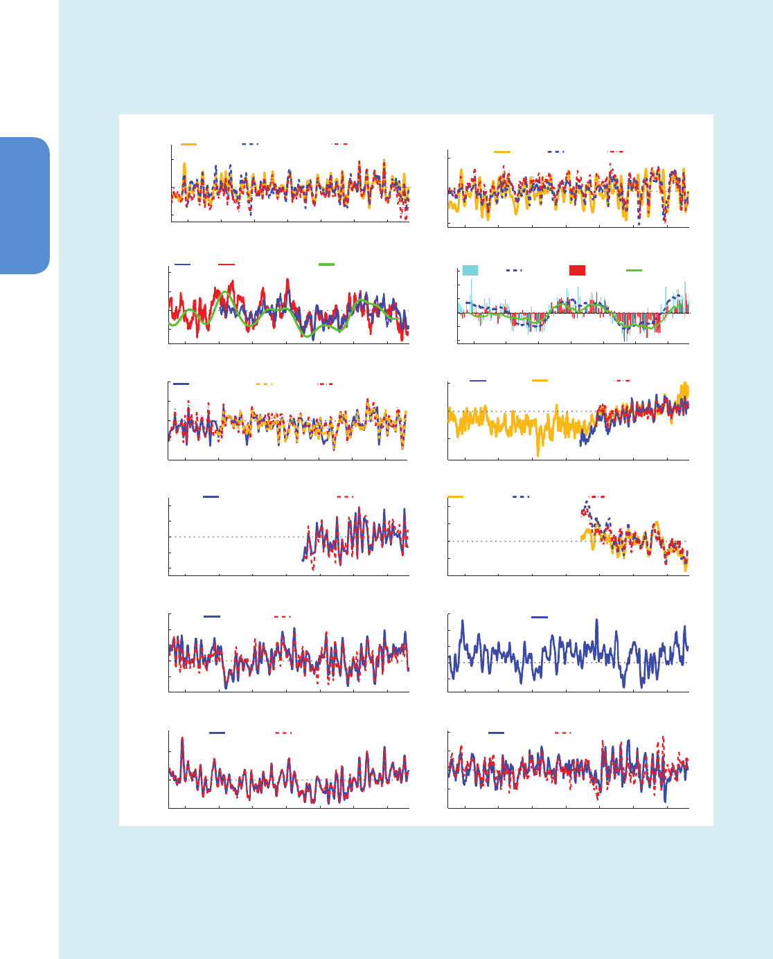
234

Chapter 2 Observations: Atmosphere and Surface

1880 1900 1920 1940 1960 1980 2000

−2

NINO3.4 (

C), SOIs (s.d.)

Traditional indices of ENSO

)r2PLSdaH()1TSSIdaH(

NINO3.4

Troup (−1)*SOI (−1)*EQSOI

880

900

960

980

000

−2

Indices (s.d.)

Additional indices of ENSO (HadISST1)

NINO4

(−1)*TNI EMI

880

900

960

980

000

−2

Indices (s.d.)

Indices of Pacific Decadal/Interdecadal Variability

r.m. (HadSLP2r)

PDO (−1)*NPI, 24−mon IPO, 11−yr LPF

880

900

960

980

000

−0.4

−0.2

0.2

0.4

0.6

Indices (

AMO indices (HadISST1): annual & 10−yr r.m.

AMO 10−yr r.m. Revised 10−yr r.m.

880

900

960

980

000

−4

−2

Indices (s.d.)

Indices of NAO and NAM/AO, DJFM means

(Hurrell,1995)

NAO stations

NAO PC NAM (HadSLP2r)

880

900

960

980

000

−2

Indices (s.d.)

Indices of SAM/AAO

(NNR) (HadSLP2r)40S−65S

Z850 PC grid 40S−70S stations

880

900

960

980

000

−2

−1

Indices (s.d.)

PNA indices, DJFM means

Centers of action (NNR)

RPC

880

900

960

980

000

−2

−1

Indices (s.d.)

PSA1 mode indices (NNR), 24−mon r.m.

PSA1 PC

Karoly PSA Yuan&Li (−1)*PSA

880

900

960

980

000

−2

−1

Indices (s.d.)

Atlantic Ocean Nino Mode indices (HadISST1)

AONM PC

ATL3 (detrended)

880

900

960

980

000

−1

AMM index (s.d.)

Tropical Atlantic Meridional Mode index (HadISST1)

AMM PC

880

900

960

980

000

−2

Indices (s.d.)

Indian Ocean Basin Mode indices (HadISST1)

IOBM PC

BMI (detrended)

880

900

960

980

000

−2

−1

Indices (s.d.)

Indian Ocean Dipole Mode indices (HadISST1)

IODM PC

DMI (detrended)

(a)

(b)

(g) (h)

(i) (j)

(k) (l)

(e) (f)

Box 2.5, Figure 1 | Some indices of climate variability, as deﬁned in Box 2.5, Table 1, plotted in the 1870–2012 interval. Where ‘HadISST1’, ‘HadSLP2r’, or ‘NNR’ are

indicated, the indices were computed from the sea surface temperature (SST) or sea level pressure (SLP) values of the former two data sets or from 500 or 850 hPa

geopotential height ﬁelds from the NNR. Data set references given in the panel titles apply to all indices shown in that panel. Where no data set is speciﬁed, a publicly

available version of an index from the authors of a primary reference given in Box 2.5, Table 1 was used. All indices were standardized with regard to 1971–2000 period

except for NIÑO3.4 (centralized for 1971–2000) and AMO indices (centralized for 1901–1970). Indices marked as “detrended” had their linear trend for 1870–2012

removed. All indices are shown as 12-month running means except when the temporal resolution is explicitly indicated (e.g., ‘DJFM’ for December-to-March averages)

or smoothing level (e.g., 11-year LPF for a low-pass ﬁlter with half-power at 11 years).

Box 2.5 (continued)

Most climate modes are illustrated by several indices (Box 2.5, Figure 1), which often behave similarly to each other. Spatial pat-

terns of SST or SLP associated with these climate modes are illustrated in Box 2.5, Figure 2. They can be interpreted as a change

in the SST or SLP ﬁeld associated with one standard deviation change in the index. (continued on next page)

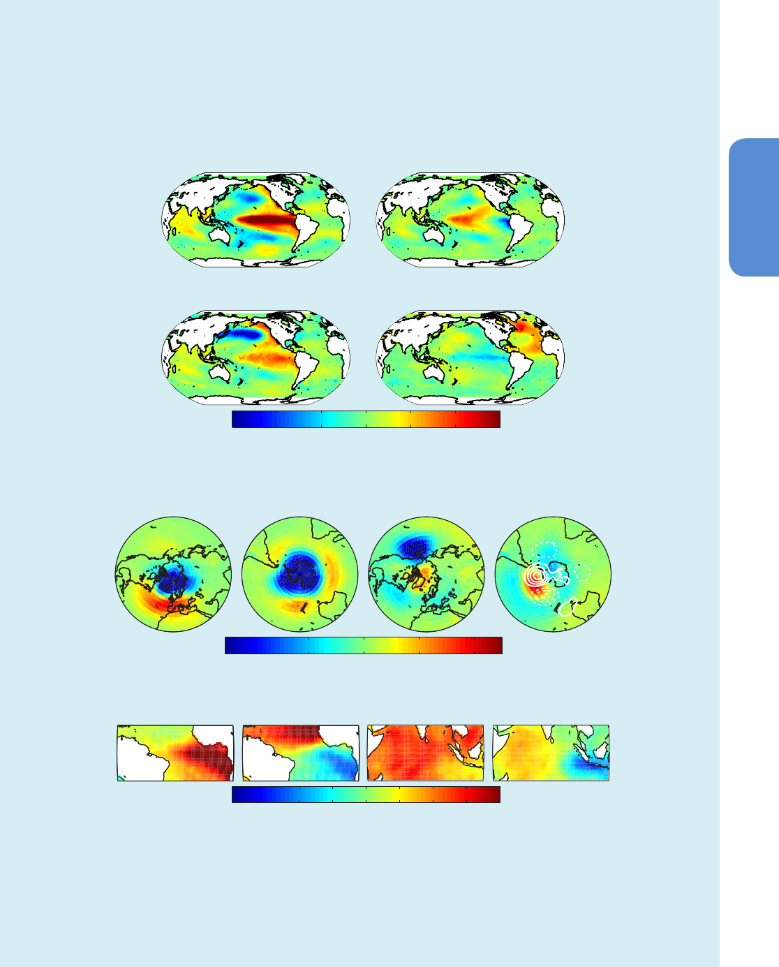
235

Observations: Atmosphere and Surface Chapter 2

El Niño – Southern Oscillation

Decadal to Multi-decadal Variability of Paciﬁc and Atlantic Oceans

SST change per index s.d. (

C per s.d.)

−0.6

−0.4 −0.2 0 0.2 0.4 0.6

Hemispheric-Scale Modes of Atmospheric Variability

MSLP change per index s.d. (hPa per s.d.)

−2 −1 0 1 2

Tropical Variability of Atlantic and Indian Oceans

−0.4

−0.3 −0.2 −0.1 0 0.1 0.2 0.3 0.4

NINO3.4 (-1)*TNI

PDO AMO (revised)

NAO

Stations (Hurrell)

SAM

Z850 PC

PNA

Centers of Action

PSA1 & PSA2

AONM ATL3 AMM PC IOBM BMI IODM DMI

SST change per index s.d. (

C per s.d.)

(a) (b)

(e) (f) (g) (h)

(i) (j) (k) (l)

Box 2.5, Figure 2 | Spatial patterns of climate modes listed in Box 2.5, Table 1. All patterns shown here are obtained by regression of either sea surface temperature

(SST) or sea level pressure (SLP) ﬁelds on the standardized index of the climate mode. For each climate mode one of the speciﬁc indices shown in Box 2.5, Figure 1 was

used, as identiﬁed in the panel subtitles. SST and SLP ﬁelds are from HadISST1 and HadSLP2r data sets (interpolated gridded products based on data sets of historical

observations). Regressions were done on monthly means for all patterns except for NAO and PNA, which were done with the DJFM means, and for PSA1 and PSA2,

where seasonal means were used. Each regression was done for the longest period within the 1870-2012 interval when the index was available. For each pattern the

time series was linearly de-trended over the entire regression interval. All patterns are shown by color plots, except for PSA2, which is shown by white contours over

the PSA1 color plot (contour steps are 0.5 hPa, zero contour is skipped, negative values are indicated by dash).

Box 2.5 (continued)

The difﬁculty of identifying a universally ‘best’ index for any particular climate mode is due to the fact that no simply deﬁned indicator

can achieve a perfect separation of the target phenomenon from all other effects occurring in the climate system. As a result, each index

is affected by many climate phenomena whose relative contributions may change with the time period and the data set used. Limited

length and quality of the observational record further compound this problem. Thus the choice of index is always application speciﬁc.

236

Chapter 2 Observations: Atmosphere and Surface

Acknowledgements

The authors of Chapter 2 wish to thank Wenche Aas (NILU, Kjeller),

Erika Coppola (ICTP, Trieste), Ritesh Gautam (NASA GSFC, Greenbelt),

Jenny Hand (CIRA, Fort Collins), Andreas Hilboll (U. Bremen, Bremen),

Glenn Hyatt (NOAA NCDC, Asheville), David Parrish (NOAA ESRL-CSD,

Boulder), Deborah Misch (LMI, Inc, Asheville), Jared Rennie (CICS-

NC, Asheville), Deborah Riddle (NOAA NCDC, Asheville), Sara Veasey

(NOAA NCDC, Asheville), Mark Weber (U. Bremen, Bremen), Yin Xun-

gang (STG Inc., Asheville), Teresa Young (STG, Asheville) and Jianglong

Zhang (U. North Dakota, Grand Forks) for their critical contributions to

the production of ﬁgures in this work.

237

Observations: Atmosphere and Surface Chapter 2

References

Abakumova, G. M., E. V. Gorbarenko, E. I. Nezval, and O. A. Shilovtseva, 2008: Fifty

years of actinometrical measurements in Moscow. Int. J. Remote Sens., 29,

2629–2665.

Adam, J. C., and D. P. Lettenmaier, 2008: Application of new precipitation and recon-

structed streamﬂow products to streamﬂow trend attribution in northern Eur-

asia. J. Clim., 21, 1807–1828.

Adler, R. F., G. J. Gu, and G. J. Huffman, 2012: Estimating climatological bias errors for

the global Precipitation Climatology Project (GPCP). J. Appl. Meteor. Climatol.,

51, 84–99.

Adler, R. F., et al., 2003: The version-2 global precipitation climatology project (GPCP)

monthly precipitation analysis (1979–present). J. Hydrometeor., 4, 1147–1167.

Aguilar, E., et al., 2009: Changes in temperature and precipitation extremes in west-

ern central Africa, Guinea Conakry, and Zimbabwe, 1955–2006. J. Geophys. Res.

Atmos., 114, D02115.

Alexander, L. V., P. Uotila, and N. Nicholls, 2009: Inﬂuence of sea surface temperature

variability on global temperature and precipitation extremes. J. Geophys. Res.

Atmos., 114, D18116.

Alexander, L. V., X. L. L. Wang, H. Wan, and B. Trewin, 2011: Signiﬁcant decline in

storminess over southeast Australia since the late 19th century. Aust. Meteor.

Ocean. J., 61, 23–30.

Alexander, L. V., et al., 2006: Global observed changes in daily climate extremes of

temperature and precipitation. J. Geophys. Res. Atmos., 111, D05109.

Allan, R., and T. Ansell, 2006: A new globally complete monthly historical gridded

mean sea level pressure dataset (HadSLP2): 1850–2004. J. Clim., 19, 5816–5842.

Allan, R., S. Tett, and L. Alexander, 2009: Fluctuations in autumn-winter severe

storms over the British Isles: 1920 to present. Int. J. Climatol., 29, 357–371.

Allan, R. P., 2009: Examination of relationships between clear-sky longwave radia-

tion and aspects of the atmospheric hydrological cycle in climate models, reanal-

yses, and observations. J. Clim., 22, 3127–3145.

Allan, R. P., and A. Slingo, 2002: Can current climate model forcings explain the

spatial and temporal signatures of decadal OLR variations? Geophys. Res. Lett.,

29, 1141.

Allan, R. P., and B. J. Soden, 2008: Atmospheric warming and the ampliﬁcation of

precipitation extremes. Science, 321, 1481–1484.

Allan, R. P., B. J. Soden, V. O. John, W. Ingram, and P. Good, 2010: Current changes in

tropical precipitation. Environ. Res. Lett., 5, 025205.

Allen, R. J., and S. C. Sherwood, 2007: Utility of radiosonde wind data in representing

climatological variations of tropospheric temperature and baroclinicity in the

western tropical Paciﬁc. J. Clim., 20, 5229–5243.

Allen, R. J., and S. C. Sherwood, 2008: Warming maximum in the tropical upper tro-

posphere deduced from thermal winds. Nature Geosci., 1, 399–403.

Alpert, P., and P. Kishcha, 2008: Quantiﬁcation of the effect of urbanization on solar

dimming. Geophys. Res. Lett., 35, L08801.

Alpert, P., P. Kishcha, Y. J. Kaufman, and R. Schwarzbard, 2005: Global dimming or

local dimming? Effect of urbanization on sunlight availability. Geophys. Res.

Lett., 32, L17802.

Andrade, C., S. Leite, and J. Santos, 2012: Temperature extremes in Europe: Over-

view of their driving atmospheric patterns. Nat. Hazards Earth Syst. Sci., 12,

1671–1691.

Andronova, N., J. E. Penner, and T. Wong, 2009: Observed and modeled evolution of

the tropical mean radiation budget at the top of the atmosphere since 1985. J.

Geophys. Res. Atmos., 114, D14106.

Angell, J. K., 2006: Changes in the 300-mb North Circumpolar Vortex, 1963–2001. J.

Clim., 19, 2984–2994.

Anthes, R. A., 2011: Exploring Earth’s atmosphere with radio occultation: contribu-

tions to weather, climate and space weather. Atmos. Meas. Tech., 4, 1077–1103.

Anthes, R. A., et al., 2008: The COSMOC/FORMOSAT-3 Mission—Early results. Bull.

Am. Meteor. Soc., 89, 313.

Archer, C. L., and K. Caldeira, 2008a: Reply to comment by Courtenay Strong and

Robert E. Davis on “Historical trends in the jet streams”. Geophys. Res. Lett.,

35. L24807.

Archer, C. L., and K. Caldeira, 2008b: Historical trends in the jet streams. Geophys.

Res. Lett., 35, L08803.

Arndt, D. S., M. O. Baringer, and M. R. Johnson, 2010: State of the Climate in 2009.

Bull. Am. Meteor. Soc., 91, S1–.

Arnold, T., et al., 2013: Nitrogen triﬂuoride global emissions estimated from updated

atmospheric measurements. Proc. Natl. Acad. Sci. U.S.A., 110, 2029–2034.

Ashok, K., S. K. Behera, S. A. Rao, H. Y. Weng, and T. Yamagata, 2007: El Niño Modoki

and its possible teleconnection. J. Geophys. Res. Oceans, 112, C11007.

Asmi, A., et al., 2013: Aerosol decadal trends – Part 2: In-situ aerosol particle number

concentrations at GAW and ACTRIS stations. Atmos. Chem. Phys., 13, 895–916.

Atlas, R., R. Hoffman, J. Ardizzone, S. Leidner, J. Jusem, D. Smith, and D. Gombos,

2011: A cross-calibrated mutiplatform ocean wind velocity product for meteor-

logical and oceanographic applications. Bull. Am. Meteor. Soc., 92, 157–.

Augustine, J. A., and E. G. Dutton, 2013: Variability of the surface radiation budget

over United States from 1996 through 2011 from high-quality measurements. J.

Geophys. Res., 118, 43-53,

Aydin, M., et al., 2011: Recent decreases in fossil-fuel emissions of ethane and meth-

ane derived from ﬁrn air. Nature, 476, 198–201.

Ballester, J., F. Giorgi, and X. Rodo, 2010: Changes in European temperature extremes

can be predicted from changes in PDF central statistics. Clim. Change, 98, 277–

284.

Baringer, M. O., D. S. Arndt, and M. R. Johnson, 2010: State of the Climate in 2009.

Bull. Am. Meteor. Soc., 91, S1–.

Barmpadimos, I., J. Keller, D. Oderbolz, C. Hueglin, and A. S. H. Prévôt, 2012: One

decade of parallel ﬁne (PM2.5) and coarse (PM10–PM2.5) particulate matter

measurements in Europe: trends and variability. Atmos. Chem. Phys., 12, 3189–

3203.

Barnston, A. G., and R. E. Livezey, 1987: Classiﬁcation, seasonality and persistence

of low-frequency atmospheric circulation patterns. Mon. Weather Rev., 115,

1083–1126.

Barring, L., and K. Fortuniak, 2009: Multi-indices analysis of southern Scandinavian

storminess 1780–2005 and links to interdecadal variations in the NW Europe-

North Sea region. Int. J. Climatol., 29, 373–384.

Barriopedro, D., E. M. Fischer, J. Luterbacher, R. Trigo, and R. Garcia-Herrera, 2011:

The hot summer of 2010: Redrawing the temperature record map of Europe.

Science, 332, 220–224.

Barrucand, M., M. Rusticucci, and W. Vargas, 2008: Temperature extremes in the

south of South America in relation to Atlantic Ocean surface temperature and

Southern Hemisphere circulation. J. Geophys. Res. Atmos., 113, D20111.

Barton, N. P., and A. W. Ellis, 2009: Variability in wintertime position and strength of

the North Paciﬁc jet stream as represented by re-analysis data. Int. J. Climatol.,

29, 851–862.

Becker, A., et al., 2013: A description of the global land-surface precipitation data

products of the Global Precipitation Climatology Centre with sample applica-

tions including centennial (trend) analysis from 1901–present. Earth Syst. Sci.

Data, 5, 71–99.

Beig, G., and V. Singh, 2007: Trends in tropical tropospheric column ozone from satel-

lite data and MOZART model. Geophys. Res. Lett., 34, L17801.

Bell, G. D., and M. S. Halpert, 1998: Climate assessment for 1997. Bull. Am. Meteor.

Soc., 79, S1–S50.

Bender, F. A. M., V. Ramanathan, and G. Tselioudis, 2012: Changes in extratropical

storm track cloudiness 1983–2008: Observational support for a poleward shift.

Clim. Dyn., 38, 2037–2053.

Bengtsson, L., and K. I. Hodges, 2011: On the evaluation of temperature trends in the

tropical troposphere. Clim. Dyn., 36, 419–430.

Beniston, M., 2004: The 2003 heat wave in Europe: A shape of things to come? An

analysis based on Swiss climatological data and model simulations. Geophys.

Res. Lett., 31, L02202.

Beniston, M., 2009: Decadal-scale changes in the tails of probability distribution

functions of climate variables in Switzerland. Int. J. Climatol., 29, 1362–1368.

Bennartz, R., J. Fan, J. Rausch, L. Leung, and A. Heidinger, 2011: Pollution from China

increases cloud droplet number, suppresses rain over the East China Sea. Geo-

phys. Res. Lett., 38, L09704.

Berrisford, P., et al., 2011: Atmospheric conservation properties in ERA-Interim. Q. J.

R. Meteor. Soc., 137, 1381–1399.

Berry, D., and E. Kent, 2011: Air-Sea ﬂuxes from ICOADS: The construction of a new

gridded dataset with uncertainty estimates. Int. J. Climatol., 31, 987–1001.

Berry, D. I., and E. C. Kent, 2009: A new air-sea interaction gridded dataset from

ICOADS with uncertainty estimates. Bull. Am. Meteor. Soc., 90, 645-656.

238

Chapter 2 Observations: Atmosphere and Surface

Berthet, C., J. Dessens, and J. Sanchez, 2011: Regional and yearly variations of hail

frequency and intensity in France. Atmos. Res., 100, 391–400.

Birner, T., 2010: Recent widening of the tropical belt from global tropopause statis-

tics: Sensitivities. J. Geophys. Res. Atmos., 115, D23109.

Bitz, C. M., and Q. Fu, 2008: Arctic warming aloft is data set dependent. Nature,

455, E3–E4.

Black, E., and R. Sutton, 2007: The inﬂuence of oceanic conditions on the hot Euro-

pean summer of 2003. Clim. Dyn., 28, 53–66.

Blunden, J., D. S. Arndt, and M. O. Baringer, 2011: State of the Climate in 2010. Bull.

Am. Meteor. Soc., 92, S17–.

Bohm, R., P. D. Jones, J. Hiebl, D. Frank, M. Brunetti, and M. Maugeri, 2010: The early

instrumental warm-bias: A solution for long central European temperature series

1760–2007. Clim. Change, 101, 41–67.

Bonﬁls, C., P. B. Duffy, B. D. Santer, T. M. L. Wigley, D. B. Lobell, T. J. Phillips, and C. Dou-

triaux, 2008: Identiﬁcation of external inﬂuences on temperatures in California.

Clim. Change, 87, S43–S55.

Bonisch, H., A. Engel, J. Curtius, T. Birner, and P. Hoor, 2009: Quantifying transport

into the lowermost stratosphere using simultaneous in-situ measurements of

and CO

. Atmos. Chem. Phys., 9, 5905–5919.

Bosilovich, M. G., F. R. Robertson, and J. Chen, 2011: Global energy and water bud-

gets in MERRA. J. Clim., 24, 5721-5739..

Bourassa, M. A., S. T. Gille, D. L. Jackson, J. B. Roberts, and G. A. Wick, 2010: Ocean

winds and turbulent air-sea ﬂuxes inferred from remote sensing. Oceanography,

23, 36–51.

Bousquet, P., 2011: Source attribution of the changes in atmospheric methane for

2006–2008. Atmos. Chem. Phys. Discuss., 10, 27603–27630.

Brogniez, H., R. Roca, and L. Picon, 2009: Study of the free tropospheric humid-

ity interannual variability using meteosat data and an advection-condensation

transport model. J. Clim., 22, 6773–6787.

Brönnimann, S., 2009: Early twentieth-century warming. Nature Geosci., 2, 735–736.

Brönnimann, S., et al., 2009: Variability of large-scale atmospheric circulation indi-

ces for the Northern Hemisphere during the past 100 years. Meteorol. Z., 18,

379–396.

Brooks, C. F., 1926: Observing water-surface temperatures at sea. Mon. Wea. Rev.,

54, 241–253.

Brooks, H., 2012: Severe thunderstorms and climate change. Atmos. Res., 123, SI,

129-138.

Brooks, H. E., and N. Dotzek, 2008: The spatial distribution of severe convective

storms and an analysis of their secular changes. In: Climate Extremes and Soci-

ety [H. F. Diaz and R. J. Murnane (eds.] Cambridge University Press, pp. 35–53.

Brown, S. J., J. Caesar, and C. A. T. Ferro, 2008: Global changes in extreme daily tem-

perature since 1950. J. Geophys. Res. Atmos., 113, D05115.

Brunet, M., et al., 2011: The minimization of the screen bias from ancient Western

Mediterranean air temperature records: an exploratory statistical analysis. Int. J.

Climatol., 31, 1879–1895.

Bunge, L., and A. J. Clarke, 2009: A veriﬁed estimation of the El Niño Index Niño-3.4

since 1877. J. Clim., 22, 3979–3992.

Burn, D. H., and N. M. Hesch, 2007: Trends in evaporation for the Canadian prairies.

J. Hydrol., 336, 61–73.

Caesar, J., L. Alexander, and R. Vose, 2006: Large-scale changes in observed daily

maximum and minimum temperatures: Creation and analysis of a new gridded

data set. J. Geophys. Res. Atmos., 111, D05101.

Caesar, J., et al., 2011: Changes in temperature and precipitation extremes over the

Indo-Paciﬁc region from 1971 to 2005. Int. J. Climatol., 31, 791–801.

Cai, W., and P. van Rensch, 2012: The 2011 southeast Queensland extreme summer

rainfall: A conﬁrmation of a negative Paciﬁc Decadal Oscillation phase? Geo-

phys. Res. Lett., 39, L08702.

Cai, W., T. Cowan, and M. Thatcher, 2012: Rainfall reductions over Southern Hemi-

sphere semi-arid regions: The role of subtropical dry zone expansion. Sci. Rep.,

2, 702.

Callaghan, J., and S. B. Power, 2011: Variability and decline in the number of severe

tropical cyclones making land-fall over eastern Australia since the late nine-

teenth century. Clim. Dyn., 37, 647–662.

Canada, 2012: Canadian Smog Science Assessment – Highlights and Key Messages.

Environment Canada and Health Canada, 64 pp.

Cane, M. A., 1986: El-Niño. Annu. Rev. Earth Planet. Sci., 14, 43–70.

Cao, Z. H., 2008: Severe hail frequency over Ontario, Canada: Recent trend and vari-

ability. Geophys. Res. Lett., 35. L14803.

Carslaw, K. S., O. Boucher, D. Spracklen, G. Mann, J. G. Rae, S. Woodward, and M.

Kumala, 2010: A review of natural aerosol interactions and feedbacks within the

Earth system. Atmos. Chem. Phys., 10, 1701–1737.

Casey, K. S., T. B. Brandon, P. Cornillon, and R. Evans, 2010: The past, present

and future of the AVHRR Pathﬁnder SST Program. In: Oceanography from

Space: Revisited [V. Barale, J. F. R. Gower, and L. Alberotanza (eds.)]. Springer

Science+Business Media, New York, 323-341.

Castellanos, P., and K. F. Boersma, 2012: Reductions in nitrogen oxides over Europe

driven by environmental policy and economic recession. Sci. Rep., 2. 265.

Cermak, J., M. Wild, R. Knutti, M. I. Mishchenko, and A. K. Heidinger, 2010: Consisten-

cy of global satellite-derived aerosol and cloud data sets with recent brightening

observations. Geophys. Res. Lett., 37, L21704.

Chambers, L., and G. Grifﬁths, 2008: The changing nature of temperature extremes in

Australia and New Zealand. Aust. Meteorol. Mag., 57, 13–35.

Chan, J. C. L., and M. Xu, 2009: Inter-annual and inter-decadal variations of landfall-

ing tropical cyclones in East Asia. Part I: time series analysis. Int. J. Climatol., 29,

1285–1293.

Chandler, R. E., and E. M. Scott, 2011: Statistical Methods for Trend Detection and

Analysis in the Environmental Sciences. John Wiley & Sons, Hoboken, NJ.

Chang, E. K. M., 2007: Assessing the increasing trend in Northern Hemisphere winter

storm track activity using surface ship observations and a statistical storm track

model. J. Clim., 20, 5607–5628.

Chang, E. K. M., and Y. J. Guo, 2007: Is the number of North Atlantic tropical cyclones

signiﬁcantly underestimated prior to the availability of satellite observations?

Geophys. Res. Lett., 34. L14801.

Chapman, W. L., and J. E. Walsh, 2007: A synthesis of Antarctic temperatures. J. Clim.,

20, 4096–4117.

Che, H. Z., et al., 2005: Analysis of 40 years of solar radiation data from China,

1961–2000. Geophys. Res. Lett., 32, L06803.

Chen, J. Y., B. E. Carlson, and A. D. Del Genio, 2002: Evidence for strengthening of the

tropical general circulation in the 1990s. Science, 295, 838–841.

Chen, J. Y., A. D. Del Genio, B. E. Carlson, and M. G. Bosilovich, 2008: The spatio-

temporal structure of twentieth-century climate variations in observations and

reanalyses. Part I: Long-term trend. J. Clim., 21, 2611–2633.

Chiacchio, M., and M. Wild, 2010: Inﬂuence of NAO and clouds on long-term sea-

sonal variations of surface solar radiation in Europe. J. Geophys. Res. Atmos.,

115, D00d22.

Choi, G., et al., 2009: Changes in means and extreme events of temperature and

precipitation in the Asia Paciﬁc Network region, 1955–2007. Int. J. Climatol.,

29, 1906–1925.

Christy, J. R., and W. B. Norris, 2006: Satellite and VIZ-radiosonde intercomparisons

for diagnosis of nonclimatic inﬂuences. J. Atmos. Ocean. Technol., 23, 1181–

1194.

Christy, J. R., and W. B. Norris, 2009: Discontinuity issues with radiosonde and satel-

lite temperatures in the Australian Region 1979–2006. J. Atmos. Ocean Technol.,

26, 508–522.

Christy, J. R., W. B. Norris, and R. T. McNider, 2009: Surface temperature variations in

East Africa and possible causes. J. Clim., 22, 3342–3356.

Christy, J. R., R. W. Spencer, and W. B. Norris, 2011: The role of remote sensing in

monitoring global bulk tropospheric temperatures. Int. J. Remote Sens., 32,

671–685.

Christy, J. R., W. B. Norris, K. Redmond, and K. P. Gallo, 2006: Methodology and

results of calculating central california surface temperature trends: Evidence of

human-induced climate change? J. Clim., 19, 548–563.

Christy, J. R., W. B. Norris, R. W. Spencer, and J. J. Hnilo, 2007: Tropospheric tempera-

ture change since 1979 from ,tropical radiosonde and satellite measurements. J.

Geophys. Res. Atmos., 112, D06102.

Christy, J. R., R. W. Spencer, W. B. Norris, W. D. Braswell, and D. E. Parker, 2003:

Error estimates of version 5.0 of MSU-AMSU bulk atmospheric temperatures. J.

Atmos. Ocean Technol., 20, 613–629.

Christy, J. R., et al., 2010: What do observational datasets say about modeled tropo-

spheric temperature trends since 1979? , 2148–2169.

Chu, W. P., M. P. McCormick, J. Lenoble, C. Brogniez, and P. Pruvost, 1989: SAGE II

inversion algorithm. J. Geophys. Res. Atmos., 94, 8339–8351.

Chung, E. S., and B. J. Soden, 2010: Investigating the inﬂuence of carbon dioxide and

the stratosphere on the long-term tropospheric temperature monitoring from

HIRS. J. Appl. Meteor. Climatol., 49, 1927–1937.

239

Observations: Atmosphere and Surface Chapter 2

Chung, E. S., D. Yeomans, and B. J. Soden, 2010: An assessment of climate feedback

processes using satellite observations of clear-sky OLR. Geophys. Res. Lett., 37,

L02702.

Clark, R. T., S. J. Brown, and J. M. Murphy, 2006: Modeling Northern Hemisphere

summer heat extreme changes and their uncertainties using a physics ensemble

of climate sensitivity experiments. J. Clim., 19, 4418–4435.

Clement, A. C., and B. Soden, 2005: The sensitivity of the tropical-mean radiation

budget. J. Clim., 18, 3189–3203.

CMA, 2007: Atlas of China Disastrous Weather and Climate. Chinese Meteorological

Administration. Beijing, China.

CMA, 2011: China Climate Change Bulletin. Chinese Meteorological Administration.

Beijing, China.

Cohen, J., M. Barlow, and K. Saito, 2009: Decadal ﬂuctuations in planetary wave

forcing modulate global warming in late boreal winter. J. Clim., 22, 4418–4426.

Cohen, J. L., J. C. Furtado, M. Barlow, V. A. Alexeev, and J. E. Cherry, 2012: Asymmetric

seasonal temperature trends. Geophys. Res. Lett., 39, L04705.

Cohn, T. A., and H. F. Lins, 2005: Nature’s style: Naturally trendy. Geophys. Res. Lett.,

32, L23402.

Coles, S., 2001: An Introduction to Statistical Modeling of Extreme Values. Springer

Science+Business Media, New York, 208 pp.

Collaud Coen, M., et al., 2013: Aerosol decadal trends – Part 1: In-situ optical mea-

surements at GAW and IMPROVE stations. Atmos. Chem. Phys., 13, 869–894.

Compo, G. P., et al., 2011: The twentieth century reanalysis project. Q. J. Roy. Meteo-

rol. Soc., 137, 1–28.

Cooper, O. R., R. S. Gao, D. Tarasick, T. Leblanc, and C. Sweeney, 2012: Long-term

ozone trends at rural ozone monitoring sites across the United States, 1990–

2010. J. Geophys. Res., 117, D22307.

Cornes, R. C., and P. D. Jones, 2011: An examination of storm activity in the northeast

Atlantic region over the 1851–2003 period using the EMULATE gridded MSLP

data series. J. Geophys. Res. Atmos., 116, D16110.

Coumou, D., A. Robinson, and S. Rahmstorf, 2013: Global increase in record-breaking

monthly-mean temperatures. Clim. Change, 118, 771-782.

Craigmile, P. F., and P. Guttorp, 2011: Space-time modelling of trends in temperature

series. J. Time Ser. Anal., 32, 378–395.

Croci-Maspoli, M., C. Schwierz, and H. C. Davies, 2007a: A multifaceted climatology

of atmospheric blocking and its recent linear trend. J. Clim., 20, 633–649.

Croci-Maspoli, M., C. Schwierz, and H. C. Davies, 2007b: Atmospheric blocking:

Space-time links to the NAO and PNA. Clim. Dyn., 29, 713–725.

Cutforth, H. W., and D. Judiesch, 2007: Long-term changes to incoming solar energy

on the Canadian Prairie. Agr. Forest Meteor., 145, 167–175.

Dai, A., 2006: Recent climatology, variability, and trends in global surface humidity.

J. Clim., 19, 3589–3606.

Dai, A., 2011a: Characteristics and trends in various forms of the Palmer Drought

Severity Index during 1900–2008. J. Geophys. Res. Atmos., 116, D12115.

Dai, A., 2012: The inﬂuence of the inter-decadal Paciﬁc oscillation on US precipitation

during 1923–2010. Clim. Dyn., 41, 633-646.

Dai, A., 2013: Increasing drought under global warming in observations and models.

Nature Clim. Change, 3, 52–58.

Dai, A., T. T. Qian, K. E. Trenberth, and J. D. Milliman, 2009: Changes in continental

freshwater diSchärge from 1948 to 2004. J. Clim., 22, 2773–2792.

Dai, A. G., 2011b: Drought under global warming: A review. Clim. Change, 2, 45–65.

Dai, A. G., J. H. Wang, P. W. Thorne, D. E. Parker, L. Haimberger, and X. L. L. Wang,

2011: A new approach to homogenize daily radiosonde humidity data. J. Clim.,

24, 965–991.

Das, L., J. D. Annan, J. C. Hargreaves, and S. Emori, 2011: Centennial scale warming

over Japan: Are the rural stations really rural? Atmos. Sci. Lett., 12, 362-367.

Davidson, E., 2009: The contribution of manure and fertilizer nitrogen to atmospher-

ic nitrous oxide since 1860. Nature Geosci., 2, 659–662.

Davini, P., C. Cagnazzo, S. Gualdi, and A. Navarra, 2012: Bidimensional diagnostics,

variability, and trends of Northern Hemisphere blocking. J. Clim., 25, 6496–6509.

Davis, S. M., and K. H. Rosenlof, 2011: A multidiagnostic intercomparison of tropi-

cal width time series using reanalyses and satellite observations. J. Clim., 25,

1061-1078.

De Laat, A. T. J., and A. N. Maurellis, 2006: Evidence for inﬂuence of anthropogenic

surface processes on lower tropospheric and surface temperature trends. Int. J.

Climatol., 26, 897–913.

de Meij, A., A. Pozzer, and J. Lelieveld, 2012: Trend analysis in aerosol optical depths

and pollutant emission estimates between 2000 and 2009. Atmos. Environ., 51,

75–85.

De Smedt, I., T. Stavrakou, J. F. Müller, R. J. van der A, and M. Van Roozendael, 2010:

Trend detection in satellite observations of formaldehyde tropospheric columns.

Geophys. Res. Lett., 37, L18808.

Dee, D. P., E. Kallen, A. J. Simmons, and L. Haimberger, 2011a: Comments on “Reanal-

yses suitable for characterizing long-term trends”. Bull. Am. Meteor. Soc., 92,

65–70.

Dee, D. P., et al., 2011b: The ERA-Interim reanalysis: Conﬁguration and performance

of the data assimilation system. Q. J. R. Meteor. Soc., 137, 553–597.

Deeds, D., et al., 2008: Evidence for crustal degassing of CF4 and SF6 in Mojave

Desert groundwaters. Geochim. Cosmochim. Acta, 72, 999–1013.

DeGaetano, A. T., 2009: Time-dependent changes in extreme-precipitation return-

period amounts in the continental United States. J. Appl. Meteor. Climatol., 48,

2086–2099.

Delgado, J. M., H. Apel, and B. Merz, 2010: Flood trends and variability in the Mekong

River. Hydrol. Earth Syst. Sci., 14, 407–418.

Della-Marta, P. M., M. R. Haylock, J. Luterbacher, and H. Wanner, 2007a: Doubled

length of western European summer heat waves since 1880. J. Geophys. Res.

Atmos., 112, D15103.

Della-Marta, P. M., J. Luterbacher, H. von Weissenﬂuh, E. Xoplaki, M. Brunet, and

H. Wanner, 2007b: Summer heat waves over western Europe 1880–2003, their

relationship to large-scale forcings and predictability. Clim. Dyn., 29, 251–275.

Della-Marta, P. M., H. Mathis, C. Frei, M. A. Liniger, J. Kleinn, and C. Appenzeller, 2009:

The return period of wind storms over Europe. Int. J. Climatol., 29, 437–459.

Deser, C., A. S. Phillips, and M. A. Alexander, 2010a: Twentieth century tropical sea

surface temperature trends revisited. Geophys. Res. Lett., 37, L10701.

Deser, C., M. A. Alexander, S. P. Xie, and A. S. Phillips, 2010b: Sea surface temperature

variability: Patterns and mechanisms. Annu. Rev. Mar. Sci., 2, 115–143.

Dessler, A. E., and S. M. Davis, 2010: Trends in tropospheric humidity from reanalysis

systems. J. Geophys. Res. Atmos., 115, D19127.

Dessler, A. E., Z. Zhang, and P. Yang, 2008: Water-vapor climate feedback inferred

from climate ﬂuctuations, 2003–2008. Geophys. Res. Lett., 35, L20704.

Diffenbaugh, N. S., J. S. Pal, F. Giorgi, and X. J. Gao, 2007: Heat stress intensiﬁcation

in the Mediterranean climate change hotspot. Geophys. Res. Lett., 34, L11706.

Ding, T., W. H. Qian, and Z. W. Yan, 2010: Changes in hot days and heat waves in

China during 1961–2007. Int. J. Climatol., 30, 1452–1462.

Ding, Y. H., G. Y. Ren, Z. C. Zhao, Y. Xu, Y. Luo, Q. P. Li, and J. Zhang, 2007: Detection,

causes and projection of climate change over China: An overview of recent prog-

ress. Adv. Atmos. Sci., 24, 954–971.

Dlugokencky, E., E. Nisbet, R. Fisher, and D. Lowry, 2011: Global atmospheric meth-

ane: Budget, changes and dangers. Philos. Trans. R. Soc. London Ser. A, 369,

2058–2072.

Dlugokencky, E., et al., 2005: Conversion of NOAA atmospheric dry air CH4 mole

fractions to a gravimetrically prepared standard scale. J. Geophys. Res. Atmos.,

110, D18306.

Dlugokencky, E., et al., 2009: Observational constraints on recent increases in the

atmospheric CH4 burden. Geophys. Res. Lett., L18803.

Dlugokencky, E. J., K. A. Masaire, P. M. Lang, P. P. Steele, and E. G. Nisbet, 1994: A

dramatic decrease in the growth rate of atmospheric methane in the Northern

Hemisphere during 1992. Geophys. Res. Lett., 21, 45–48.

Dole, R., et al., 2011: Was there a basis for anticipating the 2010 Russian heat wave?

Geophys. Res. Lett., 38, L06702.

Donat, M. G., and L. V. Alexander, 2012: The shifting probability distribution of global

daytime and night-time temperatures. Geophys. Res. Lett., 39, L14707.

Donat, M. G., D. Renggli, S. Wild, L. V. Alexander, G. C. Leckebusch, and U. Ulbrich,

2011: Reanalysis suggests long-term upward trends in European storminess

since 1871. Geophys. Res. Lett., 38, L14703.

Donat, M. G., L. V. Alexander, H. Yang, I. Durre, R. Vose, and J. Caesar, 2013a: Global

land-based datasets for monitoring climatic extremes. Bull. Am. Meteor. Soc.,

94, 997-1006.

Donat, M. G., et al., 2013b: Changes in extreme temperature and precipitation in the

Arab region: Long-term trends and variability related to ENSO and NAO. Int. J.

Climatol., doi:10.1002/joc.3707.

Donat, M. G., et al., 2013c: Updated analyses of temperature and precipitation

extreme indices since the beginning of the twentieth century: The HadEX2 data-

set. J. Geophys. Res. Atmos., 118, 2098-2118.

Dong, L., T. J. Vogelsang, and S. J. Colucci, 2008: Interdecadal trend and ENSO-related

interannual variability in Southern Hemisphere blocking. J. Clim., 21, 3068–3077.

240

Chapter 2 Observations: Atmosphere and Surface

Dorigo, W., R. de Jeu, D. Chung, R. Parinussa, Y. Liu, W. Wagner, and D. Fernández-Pri-

eto, 2012: Evaluating global trends (1988–2010) in harmonized multi-satellite

surface soil moisture. Geophys. Res. Lett., 39, L18405.

Doswell, C., H. Brooks, and N. Dotzek, 2009: On the implementation of the enhanced

Fujita scale in the USA. Atmos. Res., 93, 554–563.

Douglass, A., et al., 2008: Relationship of loss, mean age of air and the distribution

of CFCs to stratospheric circulation and implications for atmospheric lifetimes. J.

Geophys. Res. Atmos., 113, D14309.

Douglass, A., et al., 2011: WMO/UNEP scientiﬁc assessment of ozone depletion:

2010. In: Stratospheric Ozone and Surface Ultraviolet Radiation. World Meteoro-

logical Organisation, Geneva, Switzerland.

Du, Y., and S. Xie, 2008: Role of atmospheric adjustments in the tropical Indian

Ocean warming during the 20th century in climate models. Geophys. Res. Lett.,

35, L08712.

Du, Y., S. Xie, G. Huang, and K. Hu, 2009: Role of air-sea interaction in the long persis-

tence of El Niño-induced North Indian Ocean warming. J. Clim., 22, 2023–2038.

Duan, A. M., and G. X. Wu, 2006: Change of cloud amount and the climate warming

on the Tibetan Plateau. Geophys. Res. Lett., 33, L22704.

Durre, I., C. N. Williams, X. G. Yin, and R. S. Vose, 2009: Radiosonde-based trends in

precipitable water over the Northern Hemisphere: An update. J. Geophys. Res.

Atmos., 114, D05112.

Dutton, E. G., and B. A. Bodhaine, 2001: Solar irradiance anomalies caused by clear-

sky transmission variations above Mauna Loa: 1958–99. J. Clim., 14, 3255–3262.

Dutton, E. G., D. W. Nelson, R. S. Stone, D. Longenecker, G. Carbaugh, J. M. Harris, and

J. Wendell, 2006: Decadal variations in surface solar irradiance as observed in a

globally remote network. J. Geophys. Res. Atmos., 111, D19101.

Earl, N., S. Dorling, R. Hewston, and R. von Glasow, 2013: 1980–2010 Variability in

U.K. surface wind climate. J. Climate, 26, 1172–1191.

Easterling, D., and M. Wehner, 2009: Is the climate warming or cooling? Geophys.

Res. Lett., 36, L08706.

Eastman, R., and S. G. Warren, 2012: A 39-yr survey of cloud changes from land sta-

tions worldwide 1971–2009: Long-term trends, relation to aerosols, and expan-

sion of the Tropical Belt. J. Clim., 26, 1286–1303.

Eastman, R., S. G. Warren, and C. J. Hahn, 2011: Variations in cloud cover and cloud

types over the ocean from surface observations, 1954–2008. J. Clim., 24, 5914–

5934.

Ebita, A., et al., 2011: The Japanese 55-year reanalysis “JRA-55”: An interim report.

Sola, 7, 149–152.

Eccel, E., P. Cau, K. Riemann-Campe, and F. Biasioli, 2012: Quantitative hail monitor-

ing in an alpine area: 35-year climatology and links with atmospheric variables.

Int. J. Climatol., 32, 503–517.

Efthymiadis, D., C. M. Goodess, and P. D. Jones, 2011: Trends in Mediterranean grid-

ded temperature extremes and large-scale circulation inﬂuences. Nat. Hazards

Earth Syst. Sci., 11, 2199–2214.

Efthymiadis, D. A., and P. D. Jones, 2010: Assessment of maximum possible urbaniza-

tion inﬂuences on land temperature data by comparison of land and marine

data around coasts. Atmosphere, 1, 51–61.

Elkins, J. W., and G. S. Dutton, 2011: Nitrous oxide and sulfur hexaﬂouride. Bull. Am.

Meteor. Soc., 92, 2.

Elsner, J. B., J. P. Kossin, and T. H. Jagger, 2008: The increasing intensity of the stron-

gest tropical cyclones. Nature, 455, 92–95.

Emanuel, K., 2007: Environmental factors affecting tropical cyclone power dissipa-

tion. J. Clim., 20, 5497–5509.

Embury, O., and C. J. Merchant, 2011: Reprocessing for climate of sea surface tem-

perature from the along-track scanning radiometers: A new retrieval scheme.

Remote Sens. Environ., 116, 47-61.

Embury, O., C. J. Merchant, and G. K. Corlett, 2011: A reprocessing for climate of

sea surface temperature from the along-track scanning radiometers: Preliminary

validation, accounting for skin and diurnal variability. Remote Sens. Environ.,

116, 62-78.

Endo, N., and T. Yasunari, 2006: Changes in low cloudiness over China between 1971

and 1996. J. Clim., 19, 1204–1213.

Enﬁeld, D. B., A. M. Mestas-Nunez, and P. J. Trimble, 2001: The Atlantic multidecadal

oscillation and its relation to rainfall and river ﬂows in the continental US. Geo-

phys. Res. Lett., 28, 2077–2080.

Engel, A., et al., 2009: Age of stratospheric air unchanged within uncertainties over

the past 30 years. Nature Geosci., 2, 28–31.

Espinoza Villar, J. C., et al., 2009: Contrasting regional diSchärge evolutions in the

Amazon basin (1974–2004). J. Hydrol., 375, 297–311.

Etheridge, D., L. Steele, R. Francey, and R. Langenfelds, 1998: Atmospheric methane

between 1000 AD and present: Evidence of anthropogenic emissions and cli-

matic variability. J. Geophys. Res. Atmos., 15979–15993.

Etheridge, D. M., L. P. Steele, R. L. Langenfelds, R. J. Francey, J. M. Barnola, and V. I.

Morgan, 1996: Natural and anthropogenic changes in atmospheric CO

over

the last 1000 years from air in Antarctic ice and ﬁrn. J. Geophys. Res. Atmos.,

4115–4128.

Evan, A. T., A. K. Heidinger, and D. J. Vimont, 2007: Arguments against a physical

long-term trend in global ISCCP cloud amounts. Geophys. Res. Lett., 34, L04701.

Fall, S., D. Niyogi, A. Gluhovsky, R. A. Pielke, E. Kalnay, and G. Rochon, 2010: Impacts

of land use land cover on temperature trends over the continental United States:

Assessment using the North American regional reanalysis. Int. J. Climatol., 30,

1980–1993.

Fall, S., A. Watts, J. Nielsen-Gammon, E. Jones, D. Niyogi, J. R. Christy, and R. A. Pielke,

2011: Analysis of the impacts of station exposure on the US Historical Clima-

tology Network temperatures and temperature trends. J. Geophys. Res. Atmos.,

116, D14120.

Falvey, M., and R. D. Garreaud, 2009: Regional cooling in a warming world: Recent

temperature trends in the southeast Paciﬁc and along the west coast of sub-

tropical South America (1979–2006). J. Geophys. Res. Atmos., 114, D04102.

Favre, A., and A. Gershunov, 2006: Extra-tropical cyclonic/anticyclonic activity in

north-eastern Paciﬁc and air temperature extremes in western North America.

Clim. Dyn., 26, 617–629.

Feng, S., and Q. Hu, 2007: Changes in winter snowfall/precipitation ratio in the con-

tiguous United States. J. Geophys. Res. Atmos., 112, D15109.

Ferguson, C. R., and G. Villarini, 2012: Detecting inhomogeneities in the twentieth

century reanalysis over the central United States. J. Geophys. Res. Atmos., 117,

D05123.

Ferranti, L., and P. Viterbo, 2006: The European summer of 2003: Sensitivity to soil

water initial conditions. J. Clim., 19, 3659–3680.

Ferretti, D., et al., 2005: Unexpected changes to the global methane budget over the

past 2000 years. Science, 309, 1714–1717.

Fischer, E. M., and C. Schär, 2010: Consistent geographical patterns of changes in

high-impact European heatwaves. Nature Geosci., 3, 398–403.

Fischer, E. M., S. I. Seneviratne, P. L. Vidale, D. Luthi, and C. Schär, 2007: Soil mois-

ture–atmosphere interactions during the 2003 European summer heat wave. J.

Clim., 20, 5081–5099.

Fischer, T., M. Gemmer, L. Liu, and B. Su, 2011: Temperature and precipitation trends

and dryness/wetness pattern in the Zhujiang River Basin, South China, 1961–

2007. Quatern. Int., 244, 138–148.

Fogt, R. L., J. Perlwitz, A. J. Monaghan, D. H. Bromwich, J. M. Jones, and G. J. Mar-

shall, 2009: Historical SAM variability. Part II: Twentieth-century variability and

trends from reconstructions, observations, and the IPCC AR4 models. J. Clim.,

22, 5346–5365.

Folland, C. K., and D. E. Parker, 1995: Correction of instrumental biases in historical

sea-surface temperature data. Q. J. R. Meteor. Soc., 121, 319–367.

Folland, C. K., D. E. Parker, A. Colman, and W. R., 1999: Large scale modes of ocean

surface temperature since the late nineteenth century. In: Beyond El Niño:

Decadal and Interdecadal Climate Variability [A. Navarra (ed.)] Springer-Verlag,

New York, pp. 73–102.

Forster, P., et al., 2007: Changes in atmospheric constituents and in radiative forcing.

In: Climate Change 2007: The Physical Science Basis. Contribution of Working

Group I to the Fourth Assessment Report of the Intergovernmental Panel on

Climate Change [Solomon, S., D. Qin, M. Manning, Z. Chen, M. Marquis, K. B.

Averyt, M. Tignor and H. L. Miller (eds.)] Cambridge University Press, Cambridge,

United Kingdom and New York, NY, USA, 129-234.

Forster, P. M., et al., 2011: Stratospheric changes and climate. Scientiﬁc Assessment

of Ozone Depletion: 2010. Global Ozone Research and Monitoring Project–

Report No. 52. World Meteorological Organization, Geneva, Switzerland, 1-60.

Fortems-Cheiney, A., F. Chevallier, I. Pison, P. Bousquet, S. Szopa, M. N. Deeter, and C.

Clerbaux, 2011: Ten years of CO emissions as seen from Measurements of Pollu-

tion in the Troposphere (MOPITT). J. Geophys. Res., 116, D05304.

Foster, G., and S. Rahmstorf, 2011: Global temperature evolution 1979–2010. Envi-

ron. Res. Lett., 6, 044022.

Frauenfeld, O. W., and R. E. Davis, 2003: Northern Hemisphere circumpolar vortex

trends and climate change implications. J. Geophys. Res. Atmos., 108, 4423.

Frederiksen, J. S., and C. S. Frederiksen, 2007: Interdecadal changes in Southern

Hemisphere winter storm track modes. Tellus A, 59, 599–617.

241

Observations: Atmosphere and Surface Chapter 2

Free, M., and D. J. Seidel, 2007: Comments on “biases in stratospheric and tropo-

spheric temperature trends derived from historical radiosonde data”. J. Clim.,

20, 3704–3709.

Free, M., D. J. Seidel, J. K. Angell, J. Lanzante, I. Durre, and T. C. Peterson, 2005: Radio-

sonde Atmospheric Temperature Products for Assessing Climate (RATPAC): A

new data set of large-area anomaly time series. J. Geophys. Res. Atmos., 110,

D22101.

Frich, P., L. V. Alexander, P. Della-Marta, B. Gleason, M. Haylock, A. Tank, and T. Peter-

son, 2002: Observed coherent changes in climatic extremes during the second

half of the twentieth century. Clim. Res., 19, 193–212.

Fu, G. B., S. P. Charles, and J. J. Yu, 2009: A critical overview of pan evaporation trends

over the last 50 years. Clim. Change, 97, 193–214.

Fu, Q., and P. Lin, 2011: Poleward shift of subtropical jets inferred from satellite-

observed lower stratospheric temperatures. J. Clim., 24, 5597–5603.

Fu, Q., C. M. Johanson, S. G. Warren, and D. J. Seidel, 2004: Contribution of strato-

spheric cooling to satellite-inferred tropospheric temperature trends. Nature,

429, 55–58.

Fu, Q., C. M. Johanson, J. M. Wallace, and T. Reichler, 2006: Enhanced mid-latitude

tropospheric warming in satellite measurements. Science, 312, 1179–1179.

Fueglistaler, S., and P. H. Haynes, 2005: Control of interannual and longer-term vari-

ability of stratospheric water vapor. J. Geophys. Res. Atmos., 110, D24108.

Fujibe, F., 2009: Detection of urban warming in recent temperature trends in Japan.

Int. J. Climatol., 29, 1811–1822.

Fujiwara, M., et al., 2010: Seasonal to decadal variations of water vapor in the

tropical lower stratosphere observed with balloon-borne cryogenic frost point

hygrometers. J. Geophys. Res. Atmos., 115, D18304.

Fyfe, J. C., 2003: Extratropical southern hemisphere cyclones: Harbingers of climate

change? J. Clim., 16, 2802–2805.

Gallant, A., K. Hennessy, and J. Risbey, 2007: Trends in rainfall indices for six Austra-

lian regions: 1910–2005. Aust. Meteor. Mag., 56, 223–239.

Gallant, A. J. E., and D. J. Karoly, 2010: A Combined Climate Extremes Index for the

Australian Region. J. Clim., 23, 6153–6165.

Garcia-Herrera, R., J. Diaz, R. M. Trigo, J. Luterbacher, and E. M. Fischer, 2010: A

review of the European summer heat wave of 2003. Crit. Rev. Environ. Sci. Tech-

nol., 40, 267–306.

Gentemann, C., F. Wentz, C. Mears, and D. Smith, 2004: In situ validation of Tropical

Rainfall Measuring Mission microwave sea surface temperatures. J. Geophys.

Res. Oceans, 109, C04021.

Gettelman, A., and Q. Fu, 2008: Observed and simulated upper-tropospheric water

vapor feedback. J. Clim., 21, 3282–3289.

Gettelman, A., et al., 2010: Multimodel assessment of the upper troposphere and

lower stratosphere: Tropics and global trends. J. Geophys. Res. Atmos., 115,

D00M08.

Gilgen, H., A. Roesch, M. Wild, and A. Ohmura, 2009: Decadal changes in shortwave

irradiance at the surface in the period from 1960 to 2000 estimated from Global

Energy Balance Archive Data. J. Geophys. Res. Atmos., 114, D00d08.

Gillett, N. P., and P. A. Stott, 2009: Attribution of anthropogenic inﬂuence on seasonal

sea level pressure. Geophys. Res. Lett., 36, L23709.

Giorgi, F., and R. Francisco, 2000: Evaluating uncertainties in the prediction of region-

al climate change. Geophys. Res. Lett., 27, 1295–1298.

Giorgi, F., E. S. Im, E. Coppola, N. S. Diffenbaugh, X. J. Gao, L. Mariotti, and Y. Shi, 2011:

Higher hydroclimatic intensity with global warming. J. Clim., 24, 5309–5324.

Giuntoli, I., B. Renard, J. P. Vidal, and A. Bard, 2013: Low ﬂows in France and their

relationship to large-scale climate indices. J. Hydrol., 482, 105-118.

Gleason, K. L., J. H. Lawrimore, D. H. Levinson, T. R. Karl, and D. J. Karoly, 2008: A

revised US Climate Extremes Index. J. Clim., 21, 2124–2137.

Gong, D. Y., and C. H. Ho, 2002: The Siberian High and climate change over middle to

high latitude Asia. Theor. Appl. Climatol., 72, 1–9.

Gouretski, V., J. Kennedy, T. Boyer, and A. Kohl, 2012: Consistent near-surface ocean

warming since 1900 in two largely independent observing networks. Geophys.

Res. Lett., 39, L19606.

Granier, C., et al., 2011: Evolution of anthropogenic and biomass burning emissions

of air pollutants at global and regional scales during the 1980–2010 period.

Clim. Change, 109, 163–190.

Grant, A. N., S. Brönnimann, and L. Haimberger, 2008: Recent Arctic warming vertical

structure contested. Nature, 455, E2–E3.

Graversen, R. G., T. Mauritsen, M. Tjernstrom, E. Kallen, and G. Svensson, 2008: Verti-

cal structure of recent Arctic warming. Nature, 451, 53–U54.

Greally, B., et al., 2007: Observations of 1,1-diﬂuoroethane (HFC-152a) at AGAGE

and SOGE monitoring stations in 1994–2004 and derived global and regional

emission estimates. J. Geophys. Res. Atmos., 112, D06308.

Grifﬁths, G. M., et al., 2005: Change in mean temperature as a predictor of extreme

temperature change in the Asia-Paciﬁc region. Int. J. Climatol., 25, 1301–1330.

Grinsted, A., J. C. Moore, and S. Jevrejeva, 2012: Homogeneous record of Atlantic hur-

ricane surge threat since 1923. Proc. Natl. Acad. Sci. U.S.A. 109, 19601-19605.

Groisman, P., R. Knight, and T. Karl, 2012: Changes in intense precipitation over the

central United States. J. Hydrometeor., 13, 47–66.

Groisman, P., R. Knight, T. R. Karl, D. Easterling, B. M. Sun, and J. Lawrimore, 2004:

Contemporary changes of the hydrological cycle over the contiguous United

States: Trends derived from in situ observations. J. Hydrometeor., 5, 64–85.

Groisman, P. Y., R. W. Knight, D. R. Easterling, T. R. Karl, G. C. Hegerl, and V. A. N.

Razuvaev, 2005: Trends in intense precipitation in the climate record. J. Clim.,

18, 1326–1350.

Gruber, C., and L. Haimberger, 2008: On the homogeneity of radiosonde wind time

series. Meteorol. Z., 17, 631–643.

Gulev, S. K., O. Zolina, and S. Grigoriev, 2001: Extratropical cyclone variability in the

Northern Hemisphere winter from the NCEP/NCAR reanalysis data. Clim. Dyn.,

17, 795–809.

Guo, H., M. Xu, and Q. Hub, 2010: Changes in near-surface wind speed in China:

1969–2005. Int. J. Climatol., 31, 349-358.

Haerter, J., P. Berg, and S. Hagemann, 2010: Heavy rain intensity distributions on

varying time scales and at different temperatures. J. Geophys. Res. Atmos., 115,

D17102.

Haimberger, L., 2007: Homogenization of radiosonde temperature time series using

innovation statistics. J. Clim., 20, 1377–1403.

Haimberger, L., C. Tavolato, and S. Sperka, 2008: Toward elimination of the warm

bias in historic radiosonde temperature records—Some new results from a com-

prehensive intercomparison of upper-air data. J. Clim., 21, 4587–4606.

Haimberger, L., C. Tavolato, and S. Sperka, 2012: Homogenization of the global radio-

sonde temperature dataset through combined comparison with reanalysis back-

ground series and neighboring stations. J. Clim., 25, 8108–8131.

Hand, J. L., et al., 2011: IMPROVE, spatial and seasonal patterns and temporal vari-

ability of haze and its constituents in the United States. Cooperative Institute for

Research in the Atmosphere and Colorado University.

Hanna, E., J. Cappelen, R. Allan, T. Jonsson, F. Le Blancq, T. Lillington, and K. Hickey,

2008: New insights into North European and North Atlantic surface pressure

variability, storminess, and related climatic change since 1830. J. Clim., 21,

6739–6766.

Hannaford, J., and T. Marsh, 2008: High-ﬂow and ﬂood trends in a network of undis-

turbed catchments in the UK. Int. J. Climatol., 28, 1325–1338.

Hansen, J., M. Sato, and R. Ruedy, 2012: Perception of climate change. Proc. Natl.

Acad. Sci. U.S.A., 109, E2415–E2423.

Hansen, J., R. Ruedy, M. Sato, and K. Lo, 2010: Global surface temperature change.

Rev. Geophys., 48, RG4004.

Hansen, J., M. Sato, P. Kharecha, and K. von Schuckmann, 2011: Earth’s energy

imbalance and implications. Atmos. Chem. Phys., 11, 13421–13449.

Harries, J. E., and C. Belotti, 2010: On the variability of the global net radiative energy

balance of the nonequilibrium Earth. J. Clim., 23, 1277–1290.

Hatzianastassiou, N., C. Matsoukas, A. Fotiadi, K. G. Pavlakis, E. Drakakis, D. Hatzi-

dimitriou, and I. Vardavas, 2005: Global distribution of Earth’s surface shortwave

radiation budget. Atmos. Chem. Phys., 5, 2847–2867.

Hatzianastassiou, N., C. D. Papadimas, C. Matsoukas, K. Pavlakis, A. Fotiadi, M.

Wild, and I. Vardavas, 2012: Recent regional surface solar radiation dimming

and brightening patterns: inter-hemispherical asymmetry and a dimming in the

Southern Hemisphere. Atmos. Sci. Lett., 13, 43–48.

Hausfather, Z., M. J. Menne, C. N. Williams, T. Masters, R. Broberg, and D. Jones, 2013:

Quantifying the effect of urbanization on U.S. Historical Climatology Network

temperature records. J. Geophys. Res. Atmos., 118, 481-494.

Haylock, M. R., et al., 2006: Trends in total and extreme South American rainfall in

1960–2000 and links with sea surface temperature. J. Clim., 19, 1490–1512.

He, W. Y., S. P. Ho, H. B. Chen, X. J. Zhou, D. Hunt, and Y. H. Kuo, 2009: Assessment

of radiosonde temperature measurements in the upper troposphere and lower

stratosphere using COSMIC radio occultation data. Geophys. Res. Lett., 36,

L17807.

Heidinger, A. K., and M. J. Pavolonis, 2009: Gazing at cirrus clouds for 25 years

through a split window. Part I: Methodology. J. Appl. Meteor. Climatol., 48,

1100–1116.

242

Chapter 2 Observations: Atmosphere and Surface

Held, I. M., and B. J. Soden, 2006: Robust responses of the hydrological cycle to

global warming. J. Clim., 19, 5686–5699.

Helmig, D., et al., 2007: A review of surface ozone in the polar regions. Atmos. Envi-

ron., 41, 5138–5161.

Hidy, G. M., and G. T. Pennell, 2010: Multipollutant air quality management: 2010

critical review. J. Air Waste Manage. Assoc., 60, 645–674.

Hilboll, A., A. Richter, and J. P. Burrows, 2013: Long-term changes of tropospheric

over megacities derived from multiple satellite instruments. Atmos. Chem.

Phys., 13, 4145-4169.

Hinkelman, L. M., P. W. Stackhouse, B. A. Wielicki, T. P. Zhang, and S. R. Wilson, 2009:

Surface insolation trends from satellite and ground measurements: Comparisons

and challenges. J. Geophys. Res. Atmos., 114, D00d20.

Hirdman, D., et al., 2010: Long-term trends of black carbon and sulphate aerosol

in the Arctic: Changes in atmospheric transport and source region emissions.

Atmos. Chem. Phys., 10, 9351–9368.

Hirsch, M. E., A. T. DeGaetano, and S. J. Colucci, 2001: An East Coast winter storm

climatology. J. Clim., 14, 882–899.

Hirschi, M., et al., 2011: Observational evidence for soil-moisture impact on hot

extremes in southeastern Europe. Nature Geosci., 4, 17–21.

Ho, S. P., W. He, and Y. H. Kuo, 2009a: Construction of consistent temperature records

in the lower stratosphere using Global Positioning System Radio Occultation

Data and Microwave Sounding measurements. New Horizons in Occultation

Research, Springer-Verlag Berlin, 207–217.

Ho, S. P., Y. H. Kuo, Z. Zeng, and T. C. Peterson, 2007: A comparison of lower strato-

sphere temperature from microwave measurements with CHAMP GPS RO data.

Geophys. Res. Lett., 34, L15701.

Ho, S. P., M. Goldberg, Y. H. Kuo, C. Z. Zou, and W. Schreiner, 2009b: Calibration

of temperature in the lower stratosphere from microwave measurements using

COSMIC radio occultation data: Preliminary results. Terr. Atmos. Ocean. Sci., 20,

87–100.

Ho, S. P., et al., 2012: Reproducibility of GPS radio occultation data for climate moni-

toring: Proﬁle-to-proﬁle inter-comparison of CHAMP climate records 2002 to

2008 from six data centers. J. Geophys. Res. Atmos., 117, D18111.

Hoerling, M., et al., 2012: Anatomy of an extreme event. J. Clim., 26, 2811–2832.

Holben, B. N., et al., 1998: AERONET—A federated instrument network and data

archive for aerosol characterization. Remote Sens. Environ., 66, 1–16.

Holland, G. J., and P. J. Webster, 2007: Heightened tropical cyclone activity in the

North Atlantic: Natural variability or climate trend? Philos. Trans. R. Soc. London

Ser. A, 365, 2695–2716.

Hope, P. K., W. Drosdowsky, and N. Nicholls, 2006: Shifts in the synoptic systems

inﬂuencing southwest Western Australia. Clim. Dyn., 26, 751–764.

Hsu, N. C., et al., 2012: Global and regional trends of aerosol optical depth over

land and ocean using SeaWiFS measurements from 1997 to 2010. Atmos. Chem.

Phys. Discuss., 12, 8465–8501.

Hsu, P. C., T. Li, and B. Wang, 2011: Trends in global monsoon area and precipitation

over the past 30 years. Geophys. Res. Lett., 38, L08701.

Hu, Y., and Q. Fu, 2007: Observed poleward expansion of the Hadley circulation since

1979. Atmos. Chem. Phys., 7, 5229–5236.

Hu, Y. C., W. J. Dong, and Y. He, 2010: Impact of land surface forcings on mean and

extreme temperature in eastern China. J. Geophys. Res. Atmos., 115, 11.

Hu, Y. Y., C. Zhou, and J. P. Liu, 2011: Observational evidence for the poleward expan-

sion of the Hadley circulation. Adv. Atmos. Sci., 28, 33–44.

Huang, J., et al., 2008: Estimation of regional emissions of nitrous oxide from 1997

to 2005 using multinetwork measurements, a chemical transport model, and an

inverse method. J. Geophys. Res. Atmos., 113, D17313.

Huang, W.-R., S.-Y. Wang, and J. C. L. Chan, 2010: Discrepancies between global

reanalyses and observations in the interdecadal variations of Southeast Asian

cold surge. Int. J. Climatol., 31, 2272-2280..

Hudson, R. D., 2012: Measurements of the movement of the jet streams at mid-lati-

tudes, in the Northern and Southern Hemispheres, 1979 to 2010. Atmos. Chem.

Phys., 12, 7797–7808.

Hudson, R. D., M. F. Andrade, M. B. Follette, and A. D. Frolov, 2006: The total ozone

ﬁeld separated into meteorological regimes—Part II: Northern Hemisphere mid-

latitude total ozone trends. Atmos. Chem. Phys., 6, 5183–5191.

Hundecha, Y., A. St-Hilaire, T. Ouarda, S. El Adlouni, and P. Gachon, 2008: A nonsta-

tionary extreme value analysis for the assessment of changes in extreme annual

wind speed over the Gulf of St. Lawrence, Canada. J. Appl. Meteor. Climatol., 47,

2745–2759.

Hurrell, J. W., 1995: Decadal trends in the North Atlantic Oscillation: Regional tem-

peratures and precipitation. Science, 269, 676–679.

Hurst, D., 2011: Stratospheric water vapor trends over Boulder, Colorado: Analysis of

the 30 year Boulder record. J. Geophys. Res., 116, D02306.

Idso, S. B., and A. J. Brazel, 1984: Rising atmospheric carbon-dioxide concentrations

may increase streamﬂow. Nature, 312, 51–53.

IPCC, 2007: Clim. Change 2007: The Physical Science Basis. Contribution of Working

Group I to the Fourth Assessment Report of the Intergovernmental Panel on Cli-

mate Change (IPCC) [Solomon, S., D. Qin, M. Manning, Z. Chen, M. Marquis, K. B.

Averyt, M. Tignor and H. L. Miller (eds.)]. Cambridge University Press, Cambridge,

United Kingdom and New York, NY, USA, 996 pp.

Ishii, M., A. Shouji, S. Sugimoto, and T. Matsumoto, 2005: Objective analyses of sea-

surface temperature and marine meteorological variables for the 20th century

using icoads and the Kobe collection. Int. J. Climatol., 25, 865–879.

Ishijima, K., et al., 2007: Temporal variations of the atmospheric nitrous oxide con-

centration and its delta N-15 and delta O-18 for the latter half of the 20th cen-

tury reconstructed from ﬁrn air analyses. J. Geophys. Res. Atmos., 112, D03305 .

Jain, S. K., and V. Kumar, 2012: Trend analysis of rainfall and temperature data for

India. Curr. Sci., 102, 37–49.

Jakob, D., D. Karoly, and A. Seed, 2011: Non-stationarity in daily and sub-daily

intense rainfall—Part 2: Regional assessment for sites in south-east Australia.

Nat. Hazards Earth Syst. Sci., 11, 2273–2284.

Jhajharia, D., S. Shrivastava, D. Sarkar, and S. Sarkar, 2009: Temporal characteristics

of pan evaporation trends under humid conditions of northeast India. Agr. Forest

Meteorol., 336, 61–73.

Jiang, T., Z. W. Kundzewicz, and B. Su, 2008: Changes in monthly precipitation and

ﬂood hazard in the Yangtze River Basin, China. Int. J. Climatol., 28, 1471–1481.

Jiang, X., W. Ku, R. Shia, Q. Li, J. Elkins, R. Prinn, and Y. Yung, 2007: Seasonal cycle of

O: Analysis of data. Global Biogeochem. Cycles, 21, GB1006.

Jiang, Y., Y. Luo, Z. C. Zhao, and S. W. Tao, 2010: Changes in wind speed over China

during 1956–2004. Theor. Appl. Climatol., 99, 421–430.

Jin, S. G., J. U. Park, J. H. Cho, and P. H. Park, 2007: Seasonal variability of GPS-derived

zenith tropospheric delay (1994–2006) and climate implications. J. Geophys.

Res. Atmos., 112, D09110.

John, V. O., R. P. Allan, and B. J. Soden, 2009: How robust are observed and simu-

lated precipitation responses to tropical ocean warming? Geophys. Res. Lett.,

36, L14702.

John, V. O., G. Holl, R. P. Allan, S. A. Buehler, D. E. Parker, and B. J. Soden, 2011: Clear-

sky biases in satellite infrared estimates of upper tropospheric humidity and its

trends. J. Geophys. Res. Atmos., 116, D14108.

Jones, D. A., W. Wang, and R. Fawcett, 2009: High-quality spatial climate data-sets

for Australia. Australian, Meteor. Ocean. J., 58, 233–248.

Jones, P. D., and D. H. Lister, 2007: Intercomparison of four different Southern Hemi-

sphere sea level pressure datasets. Geophys. Res. Lett., 34, L10704.

Jones, P. D., and D. H. Lister, 2009: The urban heat island in Central London and

urban-related warming trends in Central London since 1900. Weather, 64,

323–327.

Jones, P. D., T. Jonsson, and D. Wheeler, 1997: Extension to the North Atlantic Oscil-

lation using early instrumental pressure observations from Gibraltar and south-

west Iceland. Int. J. Climatol., 17, 1433–1450.

Jones, P. D., D. H. Lister, and Q. Li, 2008: Urbanization effects in large-scale tempera-

ture records, with an emphasis on China. J. Geophys. Res. Atmos., 113, D16122.

Jones, P. D., D. H. Lister, T. J. Osborn, C. Harpham, M. Salmon, and C. P. Morice, 2012:

Hemispheric and large-scale land-surface air temperature variations: An exten-

sive revision and an update to 2010. J. Geophys. Res. Atmos., 117, D05127.

Jones, R., S. Westra, and A. Sharma, 2010: Observed relationships between extreme

sub-daily precipitation, surface temperature, and relative humidity. Geophys.

Res. Lett., 37, L22805.

Joshi, M. M., J. M. Gregory, M. J. Webb, D. M. H. Sexton, and T. C. Johns, 2008: Mecha-

nisms for the land/sea warming contrast exhibited by simulations of climate

change. Clim. Dyn., 30, 455–465.

Jovanovic, B., D. Collins, K. Braganza, D. Jakob, and D. A. Jones, 2011: A high-quality

monthly total cloud amount dataset for Australia. Clim. Change, 108, 485-517.

Jung, M., et al., 2010: Recent decline in the global land evapotranspiration trend due

to limited moisture supply. Nature, 467, 951–954.

Kahn, R. A., et al., 2007: Satellite-derived aerosol optical depth over dark water from

MISR and MODIS: Comparisons with AERONET and implications for climatologi-

cal studies. J. Geophys. Res. Atmos., 112, D18205.

243

Observations: Atmosphere and Surface Chapter 2

Kanamitsu, M., W. Ebisuzaki, J. Woollen, S. K. Yang, J. J. Hnilo, M. Fiorino, and G.

L. Potter, 2002: NCEP-DOE AMIP-II reanalysis (R-2). Bull. Am. Meteor. Soc., 83,

1631–1643.

Kang, S. M., L. M. Polvani, J. C. Fyfe, and M. Sigmond, 2011: Impact of polar ozone

depletion on subtropical Precipitation. Science, 332, 951–954.

Kao, H. Y., and J. Y. Yu, 2009: Contrasting Eastern-Paciﬁc and Central-Paciﬁc types of

ENSO. J. Clim., 22, 615–632.

Karnauskas, K. B., R. Seager, A. Kaplan, Y. Kushnir, and M. A. Cane, 2009: Observed

strengthening of the zonal sea surface temperature gradient across the equato-

rial Paciﬁc Ocean. J. Clim., 22, 4316–4321.

Karnieli, A., et al., 2009: Temporal trend in anthropogenic sulfur aerosol transport

from central and eastern Europe to Israel. J. Geophys. Res. Atmos., 114, D00d19.

Karoly, D., 1989: Southern-Hemisphere circulation features associated with El Niño-

Southern Oscillation. J. Clim., 2, 1239–1252.

Kato, S., et al.: Surface irradiances consistent with CERES-derived top-of-atmosphere

shortwave and longwave irradiances. J. Clim. 26, 2719-2740

Keeling, C., R. Bacastow, A. Bainbridge, C. Ekdahl, P. Guenther, L. Waterman, and

J. Chin, 1976a: Atmospheric Carbon-Dioxide Variations at Mauna-Loa Observa-

tory, Hawaii. Tellus, 28, 538–551.

Keeling, C. D., J. A. Adams, and C. A. Ekdahl, 1976b: Atmospheric carbo-dioxide varia-

tions at South Pole. Tellus, 28, 553–564.

Keller, C., D. Brunner, S. Henne, M. Vollmer, S. O’Doherty, and S. Reimann, 2011: Evi-

dence for under-reported western European emissions of the potent greenhouse

gas HFC-23. Geophys. Res. Lett., 38, L15808.

Kennedy, J. J., N. A. Rayner, and R. O. Smith, 2012: Using AATSR data to assess the

quality of in situ sea surface temperature observations for climate studies.

Remote Sens. Environ., 116, 79–92.

Kennedy, J. J., N. A. Rayner, R. O. Smith, D. E. Parker, and M. Saunby, 2011a: Reas-

sessing biases and other uncertainties in sea surface temperature observations

measured in situ since 1850: 2. Biases and homogenization. J. Geophys. Res.

Atmos., 116, D14104.

Kennedy, J. J., N. A. Rayner, R. O. Smith, M. Saunby, and D. E. Parker, 2011b: Reas-

sessing biases and other uncertainties in sea surface temperature observations

since 1850, part 1: Measurement and sampling uncertainties. J. Geophys. Res.,

116, D14103.

Kent, E. C., and D. I. Berry, 2008: Assessment of the Marine Observing System

(ASMOS): Final report. National Oceanography Centre Southampton Research

and Consultancy Report, 55 pp.

Kent, E. C., S. D. Woodruff, and D. I. Berry, 2007: Metadata from WMO publication

no. 47 and an assessment of voluntary observing ship observation heights in

ICOADS. J. Atmos. Ocean Technol., 24, 214–234.

Kent, E. C., S. Fangohr, and D. I. Berry, 2012: A comparative assessment of monthly

mean wind speed products over the global ocean. Int. J. Climatol., 33, 2530-

2541.

Kent, E. C., J. J. Kennedy, D. I. Berry, and R. O. Smith, 2010: Effects of instrumenta-

tion changes on sea surface temperature measured in situ. Clim. Change, 1,

718–728.

Kent, E. C., N. A. Rayner, D. I. Berry, M. Saunby, B. I. Moat, J. J. Kennedy, and D. E.

Parker, 2013: Global analysis of night marine air temperature and its uncertainty

since 1880, the HadNMAT2 Dataset, J. Geophys. Res., 118, 1281-1298.

Kenyon, J., and G. C. Hegerl, 2008: Inﬂuence of modes of climate variability on global

temperature extremes. J. Clim., 21, 3872–3889.

Kenyon, J., and G. C. Hegerl, 2010: Inﬂuence of modes of climate variability on global

precipitation extremes. J. Clim., 23, 6248–6262.

Kharin, V., F. Zwiers, X. Zhang, and M. Wehner, 2013: Changes in temperature and

precipitation extremes in the CMIP5 ensemble. Climatic Change, 119, 345-357.

Kiehl, J. T., and K. E. Trenberth, 1997: Earth’s annual global mean energy budget. Bull.

Am. Meteor. Soc., 78, 197–208.

Kim, D., and V. Ramanathan, 2012: Improved estimates and understanding of global

albedo and atmospheric solar absorption. Geophys. Res. Lett., 39, L24704.

Kim, D. Y., and V. Ramanathan, 2008: Solar radiation budget and radiative forcing

due to aerosols and clouds. J. Geophys. Res. Atmos., 113, D02203.

Kim, J., et al., 2010: Regional atmospheric emissions determined from measure-

ments at Jeju Island, Korea: Halogenated compounds from China. Geophys. Res.

Lett., 37, L12801.

King, A., L. Alexander, and M. Donat, 2013: The efﬁcacy of using gridded data to

examine extreme rainfall characteristics: A case study for Australia. Inter. J. Cli-

matol., 33, 2376-2387.

Kistler, R., et al., 2001: The NCEP-NCAR 50-year reanalysis: Monthly means CD-ROM

and documentation. Bull. Am. Meteor. Soc., 82, 247–267.

Klein Tank, A. M. G., et al., 2006: Changes in daily temperature and precipitation

extremes in central and south Asia. J. Geophys. Res. Atmos., 111, D16105.

Klok, E. J., and A. Tank, 2009: Updated and extended European dataset of daily cli-

mate observations. Int. J. Climatol., 29, 1182–1191.

Knapp, K. R., and M. C. Kruk, 2010: Quantifying interagency differences in tropical

cyclone best-track wind speed estimates. Mon. Weather Rev., 138, 1459–1473.

Knowles, N., M. D. Dettinger, and D. R. Cayan, 2006: Trends in snowfall versus rainfall

in the western United States. J. Clim., 19, 4545–4559.

Knutson, T. R., et al., 2010: Tropical cyclones and climate change. Nature Geosci., 3,

157–163.

Kobayashi, S., M. Matricardi, D. Dee, and S. Uppala, 2009: Toward a consistent reanal-

ysis of the upper stratosphere based on radiance measurements from SSU and

AMSU-A. Q. J. R. Meteorol. Soc., 135, 2086–2099.

Kopp, G., and G. Lawrence, 2005: The Total Irradiance Monitor (TIM): Instrument

design. Solar Phys., 230, 91–109.

Kopp, G., and J. L. Lean, 2011: A new, lower value of total solar irradiance: Evidence

and climate signiﬁcance. Geophys. Res. Lett., 38, L01706.

Kopp, G., G. Lawrence, and G. Rottman, 2005: The Total Irradiance Monitor (TIM):

Science results. Solar Phys., 230, 129–139.

Kossin, J. P., K. R. Knapp, D. J. Vimont, R. J. Murnane, and B. A. Harper, 2007: A glob-

ally consistent reanalysis of hurricane variability and trends. Geophys. Res. Lett.,

34, L04815.

Koutsoyiannis, D., and A. Montanari, 2007: Statistical analysis of hydroclimatic time

series: Uncertainty and insights. Water Resour. Res., 43, W05429.

Kreienkamp, F., A. Spekat, and W. Enke, 2010: Stationarity of atmospheric waves and

blocking over Europe-based on a reanalysis dataset and two climate scenarios.

Theor. Appl. Climatol., 102, 205–212.

Krishna Moorthy, K., S. Suresh Babu, and S. K. Satheesh, 2007: Temporal heteroge-

neity in aerosol characteristics and the resulting radiative impact at a tropical

coastal station—Part 1: Microphysical and optical properties. Ann. Geophys.,

25, 2293–2308.

Krishna Moorthy, K., S. Suresh Babu, M. R. Manoj, and S. K. Satheesh, 2013: Buildup

of Aerosols over the Indian Region. Geophys. Res. Lett., 40, 1011-1014

Krishna Moorthy, K., S. S. Babu, S. K. Satheesh, S. Lal, M. M. Sarin, and S. Ramach-

andran, 2009: Climate implications of atmospheric aerosols and trace gases:

Indian Scenario, Climate Sense. World Meteorological Organisation, Geneva,

Switzerland, pp. 157–160.

Krueger, O., F. Schenk, F. Feser, and R. Weisse, 2013: Inconsistencies between long-

term trends in storminess derived from the 20CR reanalysis and observations. J.

Clim., 26, 868–874.

Kruger, A., and S. Sekele, 2013: Trends in extreme temperature indices in South

Africa: 1962–2009. Int. J. Climatol., 33, 661-676.

Kubota, H., and J. C. L. Chan, 2009: Interdecadal variability of tropical cyclone land-

fall in the Philippines from 1902 to 2005. Geophys. Res. Lett., 36, L12802.

Kudo, R., A. Uchiyama, A. Yamazaki, T. Sakami, and O. Ijima, 2011: Decadal changes

in aerosol optical thickness and single scattering albedo estimated from ground-

based broadband radiometers: A case study in Japan. J. Geophys. Res., 116,

D03207.

Kudo, R., A. Uchiyama, O. Ijima, N. Ohkawara, and S. Ohta, 2012: Aerosol impact on

the brightening in Japan. J. Geophys. Res. Atmos., 117, 11.

Kueppers, L. M., M. A. Snyder, and L. C. Sloan, 2007: Irrigation cooling effect: Region-

al climate forcing by land-use change. Geophys. Res. Lett., 34, L03703.

Kuglitsch, F. G., A. Toreti, E. Xoplaki, P. M. Della-Marta, J. Luterbacher, and H. Wanner,

2009: Homogenization of daily maximum temperature series in the Mediter-

ranean. J. Geophys. Res. Atmos., 114, D15108.

Kuglitsch, F. G., A. Toreti, E. Xoplaki, P. M. Della-Marta, C. S. Zerefos, M. Turkes, and J.

Luterbacher, 2010: Heat wave changes in the eastern Mediterranean since 1960.

Geophys. Res. Lett., 37, L04802.

Kumari, B. P., and B. N. Goswami, 2010: Seminal role of clouds on solar dimming over

the Indian monsoon region. Geophys. Res. Lett., 37, L06703.

Kumari, B. P., A. L. Londhe, S. Daniel, and D. B. Jadhav, 2007: Observational evidence

of solar dimming: Offsetting surface warming over India. Geophys. Res. Lett.,

34, L21810.

244

Chapter 2 Observations: Atmosphere and Surface

Kundzewicz, Z. W., et al., 2007: Freshwater resources and their management. Cli-

mate Change 2007: Impacts, Adaptation and Vulnerability. Contribution of

Working Group II to the Fourth Assessment Report of the Intergovernmental

Panel on Climate Change [Solomon, S., D. Qin, M. Manning, Z. Chen, M. Marquis,

K. B. Averyt, M. Tignor and H. L. Miller (eds.)].Cambridge University Press, Cam-

bridge, United Kingdom and New York, NY, USA,172-210.

Kunkel, K. E., M. A. Palecki, L. Ensor, D. Easterling, K. G. Hubbard, D. Robinson, and

K. Redmond, 2009: Trends in twentieth-century US extreme snowfall seasons. J.

Clim., 22, 6204–6216.

Kunkel, K. E., et al., 2008: Observed changes in weather and climate extremes. In:

Weather and Climate Extremes in a Changing Climate. Regions of Focus: North

America, Hawaii, Caribbean, and U.S. Paciﬁc Islands [T. R. Karl, G. A. Meehl, D. M.

Christopher, S. J. Hassol, A. M. Waple, and W. L. Murray (eds.)]. A Report by the

U.S. Climate Change Science Program and the Subcommittee on Global Change

Research.

Kunz, M., J. Sander, and C. Kottmeier, 2009: Recent trends of thunderstorm and hail-

storm frequency and their relation to atmospheric characteristics in southwest

Germany. Int. J. Climatol., 29, 2283–2297.

Kuo, Y. H., W. S. Schreiner, J. Wang, D. L. Rossiter, and Y. Zhang, 2005: Comparison

of GPS radio occultation soundings with radiosondes. Geophys. Res. Lett., 32,

L05817.

Kvalevag, M. M., and G. Myhre, 2007: Human impact on direct and diffuse solar

radiation during the industrial era. J. Clim., 20, 4874–4883.

L’Ecuyer, T. S., N. B. Wood, T. Haladay, G. L. Stephens, and P. W. Stackhouse, 2008:

Impact of clouds on atmospheric heating based on the R04 CloudSat ﬂuxes and

heating rates data set. J. Geophys. Res. Atmos., 113, 15.

Labat, D., Y. Godderis, J. L. Probst, and J. L. Guyot, 2004: Evidence for global runoff

increase related to climate warming. Adv. Water Resour., 27, 631–642.

Ladstadter, F., A. K. Steiner, U. Foelsche, L. Haimberger, C. Tavolato, and G. Kirch-

nebngast, 2011: An assessment of differences in lower stratospheric tempera-

ture records from (A)MSU, radiosondes and GPS radio occultation. Atmos. Meas.

Tech., 4, 1965–1977.

Landsea, C. W., 2007: Counting Atlantic tropical cyclones back to 1900. EOS Trans.

(AGU), 88, 197–202.

Landsea, C. W., B. A. Harper, K. Hoarau, and J. A. Knaff, 2006: Can we detect trends

in extreme tropical cyclones? Science, 313, 452–454.

Landsea, C. W., et al., 2011: A reanalysis of the 1921–30 Atlantic Hurricane Data-

base. J. Clim., 25, 865–885.

Langematz, U., and M. Kunze, 2008: Dynamical changes in the Arctic and Antarctic

stratosphere during spring. In: Climate Variability and Extremes during the Past

100 Years. Advances in Global Change Research [S. Brönnimann, J. Luterbacher, T.

Ewen, H. F. Diaz, R. S. Stolarski, and U. Neu (eds.)], Springer, pp. 293–301.

Lanzante, J. R., 2009: Comment on “Trends in the temperature and water vapor

content of the tropical lower stratosphere: Sea surface connection” by Karen H.

Rosenlof and George C. Reid. J. Geophys. Res. Atmos., 114, D12104.

Laprise, R., 1992: The resolution of global spectroal models. Bull. Am. Meteor. Soc.,

73, 1453–1454.

Larkin, N. K., and D. E. Harrison, 2005: On the deﬁnition of El Niño and associated

seasonal average US weather anomalies. Geophys. Res. Lett., 32, L13705.

Lawrimore, J. H., M. J. Menne, B. E. Gleason, C. N. Williams, D. B. Wuertz, R. S. Vose,

and J. Rennie, 2011: An overview of the Global Historical Climatology Network

monthly mean temperature data set, version 3. J. Geophys. Res. Atmos., 116,

D19121.

Leakey, A. D. B., M. Uribelarrea, E. A. Ainsworth, S. L. Naidu, A. Rogers, D. R. Ort, and

S. P. Long, 2006: Photosynthesis, productivity, and yield of maize are not affected

by open-air elevation of CO

concentration in the absence of drought. Plant

Physiol., 140, 779–790.

Lee, H. T., A. Gruber, R. G. Ellingson, and I. Laszlo, 2007: Development of the HIRS

outgoing longwave radiation climate dataset. J. Atmos. Ocean Technol., 24,

2029–2047.

Lefohn, A. S., D. Shadwick, and S. J. Oltmans, 2010: Characterizing changes in surface

ozone levels in metropolitan and rural areas in the United States for 1980–2008

and 1994–2008. Atmos. Environ., 44, 5199–5210.

Lehmann, A., K. Getzlaff, and J. Harlass, 2011: Detailed assessment of climate vari-

ability in the Baltic Sea area for the period 1958 to 2009. Clim. Res., 46, 185–

196.

Lelieveld, J., J. van Aardenne, H. Fischer, M. de Reus, J. Williams, and P. Winkler, 2004:

Increasing ozone over the Atlantic Ocean. Science, 304, 1483–1487.

Lenderink, G., and E. Van Meijgaard, 2008: Increase in hourly precipitation extremes

beyond expectations from temperature changes. Nature Geosci., 1, 511–514.

Lenderink, G., H. Y. Mok, T. C. Lee, and G. J. van Oldenborgh, 2011: Scaling and trends

of hourly precipitation extremes in two different climate zones – Hong

Kong and the Netherlands. Hydrol. Earth Syst. Sci. Discuss., 8, 4701–4719.

Lennartz, S., and A. Bunde, 2009: Trend evaluation in records with long-term memory:

Application to global warming. Geophys. Res. Lett., 36, L16706.

Levin, I., et al., 2010: The global SF6 source inferred from long-term high preci-

sion atmospheric measurements and its comparison with emission inventories.

Atmos. Chem. Phys., 10, 2655–2662.

Levitus, S., J. I. Antonov, T. P. Boyer, R. A. Locarnini, H. E. Garcia, and A. V. Mishonov,

2009: Global ocean heat content 1955–2008 in light of recently revealed instru-

mentation problems. Geophys. Res. Lett., 36, 5.

Levy, R. C., L. A. Remer, R. G. Kleidman, S. Mattoo, C. Ichoku, R. Kahn, and T. F. Eck,

2010: Global evaluation of the Collection 5 MODIS dark-target aerosol products

over land. Atmos. Chem. Phys., 10, 10399–10420.

Li, Q., H. Zhang, X. Liu, J. Chen, W. Li, and P. Jones, 2009: A mainland China homog-

enized historical temperature dataset of 1951–2004. Bull. Am. Meteor. Soc., 90,

1062–1065.

Li, Q., W. Dong, W. Li, X. Gao, P. Jones, J. Kennedy, and D. Parker, 2010a: Assessment of

the uncertainties in temperature change in China during the last century. Chin.

Sci. Bull., 55, 1974–1982.

Li, Q. X., et al., 2010b: Assessment of surface air warming in northeast China, with

emphasis on the impacts of urbanization. Theor. Appl. Climatol., 99, 469–478.

Li, Z., et al., 2012: Changes of daily climate extremes in southwestern China during

1961–2008. Global Planet. Change, 80–81, 255–272.

Liang, F., and X. A. Xia, 2005: Long-term trends in solar radiation and the associated

climatic factors over China for 1961–2000. Ann. Geophys., 23, 2425–2432.

Liebmann, B., R. M. Dole, C. Jones, I. Blade, and D. Allured, 2010: Inﬂuence of choice

of time period on global surface temperature trend estimates. Bull. Am. Meteor.

Soc., 91, 1485–U1471.

Liepert, B. G., 2002: Observed reductions of surface solar radiation at sites in the

United States and worldwide from 1961 to 1990. Geophys. Res. Lett., 29, 1421.

Liley, J. B., 2009: New Zealand dimming and brightening. J. Geophys. Res. Atmos.,

114, D00d10.

Lim, E. P., and I. Simmonds, 2007: Southern Hemisphere winter extratropical cyclone

characteristics and vertical organization observed with the ERA-40 data in

1979–2001. J. Clim., 20, 2675–2690.

Lim, E. P., and I. Simmonds, 2009: Effect of tropospheric temperature change on the

zonal mean circulation and SH winter extratropical cyclones. Clim. Dyn., 33,

19–32.

Lim, Y. K., M. Cai, E. Kalnay, and L. Zhou, 2008: Impact of vegetation types on surface

temperature change. J. Appl. Meteor. Climatol., 47, 411–424.

Lin, C., K. Yang, J. Qin, and R. Fu, 2012: Observed coherent trends of surface and

upper-air wind speed over China since 1960. J. Clim.,26, 2891-2903..

Liu, B., M. Xu, and M. Henderson, 2011: Where have all the showers gone? Regional

declines in light precipitation events in China, 1960–2000. Int. J. Climatol., 31,

1177–1191.

Liu, B. H., M. Xu, M. Henderson, and W. G. Gong, 2004a: A spatial analysis of pan

evaporation trends in China, 1955–2000. J. Geophys. Res. Atmos., 109, D15102.

Liu, B. H., M. Xu, M. Henderson, Y. Qi, and Y. Q. Li, 2004b: Taking China’s temperature:

Daily range, warming trends, and regional variations, 1955–2000. J. Clim., 17,

4453–4462.

Liu, Q. H., and F. Z. Weng, 2009: Recent stratospheric temperature observed from

satellite measurements. Sola, 5, 53–56.

Lo, M.-H., and J. S. Famiglietti, 2013: Irrigation in California’s Central Valley strength-

ens the southwestern U.S. water cycle. Geophys. Res. Lett., 40, 301-306.

Loeb, N. G., et al., 2009: Toward optimal closure of the Earth’s top-of-atmosphere

radiation budget. J. Clim., 22, 748–766.

Loeb, N. G., et al., 2012a: Advances in understanding top-of-atmosphere radiation

variability from satellite observations. Surv. Geophys., 33, 359–385.

Loeb, N. G., et al., 2012b: Observed changes in top-of-the-atmosphere radiation and

upper-ocean heating consistent within uncertainty. Nature Geosci., 5, 110–113.

Logan, J. A., et al., 2012: Changes in ozone over Europe since 1990: Analysis of ozone

measurements from sondes, regular aircraft (MOZAIC), and alpine surface sites.

J. Geophys. Res., 117, D09301.

Long, C. N., E. G. Dutton, J. A. Augustine, W. Wiscombe, M. Wild, S. A. McFarlane, and

C. J. Flynn, 2009: Signiﬁcant decadal brightening of downwelling shortwave in

the continental United States. J. Geophys. Res. Atmos., 114, D00d06.

245

Observations: Atmosphere and Surface Chapter 2

Lorenz, R., E. B. Jaeger, and S. I. Seneviratne, 2010: Persistence of heat waves and its

link to soil moisture memory. Geophys. Res. Lett., 37, L09703.

Lucas, C., H. Nguyen, and B. Timbal, 2012: An observational analysis of Southern

Hemispheretropical expansion. J. Geohys. Res., 117, D17112.

Luo, J. J., W. Sasaki, and Y. Masumoto, 2012: Indian Ocean warming modulates Paciﬁc

climate change. Proc. Natl. Acad. Sci. U.S.A., 109, 18701–18706.

Lupikasza, E., 2010: Spatial and temporal variability of extreme precipitation in

Poland in the period 1951–2006. Int. J. Climatol., 30, 991–1007.

Lyman, J. M., et al., 2010: Robust warming of the global upper ocean. Nature, 465,

334–337.

Lynch, A. H., J. A. Curry, R. D. Brunner, and J. A. Maslanik, 2004: Toward an integrated

assessment of the impacts of extreme wind events on Barrow, Alaska. Bull. Am.

Meteor. Soc., 85, 209–.

Mahowald, N., et al., 2010: Observed 20th century desert dust variability: Impact on

climate and biogeochemistry. Atmos. Chem. Phys., 10, 10875–10893.

Makowski, K., M. Wild, and A. Ohmura, 2008: Diurnal temperature range over

Europe between 1950 and 2005. Atmos. Chem. Phys., 8, 6483–6498.

Makowski, K., E. B. Jaeger, M. Chiacchio, M. Wild, T. Ewen, and A. Ohmura, 2009: On

the relationship between diurnal temperature range and surface solar radiation

in Europe. J. Geophys. Res. Atmos., 114, D00d07.

Manabe, S., and R. F. Strickler, 1964: Thermal equilibrium of the atmosphere with

a convective adjustment. Journal of the Atmospheric Sciences, 21, 361–385.

Mann, M. E., 2011: On long range dependence in global surface temperature series.

Clim. Change, 107, 267–276.

Mann, M. E., T. A. Sabbatelli, and U. Neu, 2007a: Evidence for a modest undercount

bias in early historical Atlantic tropical cyclone counts. Geophys. Res. Lett., 34,

L22707.

Mann, M. E., K. A. Emanual, G. J. Holland, and P. J. Webster, 2007b: Atlantic tropical

cyclones revisited. EOS Transactions (AGU), 88, 349–350.

Manney, G. L., et al., 2011: Unprecedented Arctic ozone loss in 2011. Nature, 478,

469–475.

Mantua, N. J., S. R. Hare, Y. Zhang, J. M. Wallace, and R. C. Francis, 1997: A Paciﬁc

interdecadal climate oscillation with impacts on salmon production. Bull. Am.

Meteor. Soc., 78, 1069–1079.

Marenco, A., H. Gouget, P. Nédélec, and J. P. Pagés, 1994: Evidence of a long-term

increase in tropospheric ozone from Pic du Midi series: Consequences: positive

radiative forcing. J. Geophys. Res., 99, 16,617–616, 632.

Marshall, G. J., 2003: Trends in the southern annular mode from observations and

reanalyses. J. Clim., 16, 4134–4143.

Martinerie, P., et al., 2009: Long-lived halocarbon trends and budgets from atmo-

spheric chemistry modelling constrained with measurements in polar ﬁrn.

Atmos. Chem. Phys., 3911–3934.

Mastrandrea, M., et al., 2011: The IPCC AR5 guidance note on consistent treatment

of uncertainties: A common approach across the working groups. Clim. Change,

108, 675–691.

Matulla, C., W. Schoner, H. Alexandersson, H. von Storch, and X. L. Wang, 2008: Euro-

pean storminess: Late nineteenth century to present. Clim. Dyn., 31, 125–130.

McCarthy, M. P., P. W. Thorne, and H. A. Titchner, 2009: An analysis of tropospheric

humidity trends from radiosondes. J. Clim., 22, 5820–5838.

McCarthy, M. P., H. A. Titchner, P. W. Thorne, S. F. B. Tett, L. Haimberger, and D. E.

Parker, 2008: Assessing bias and uncertainty in the HadAT-adjusted radiosonde

climate record. J. Clim., 21, 817–832.

McKitrick, R., 2010: Atmospheric circulations do not explain the temperature-indus-

trialization correlation. Stat. Politics Policy, 1, issue 1 .

McKitrick, R., and P. J. Michaels, 2004: A test of corrections for extraneous signals in

gridded surface temperature data. Clim. Res., 26, 159–173.

McKitrick, R., and N. Nierenberg, 2010: Socioeconomic patterns in climate data. J.

Econ. Soc. Meas, 35, 149–175.

McKitrick, R. R., and P. J. Michaels, 2007: Quantifying the inﬂuence of anthropogenic

surface processes and inhomogeneities on gridded global climate data. J. Geo-

phys. Res. Atmos., 112, D24S09.

McNider, R. T., et al., 2012: Response and sensitivity of the nocturnal boundary layer

over land to added longwave radiative forcing. J. Geophys. Res., 117, D14106.

McVicar, T. R., T. G. Van Niel, L. T. Li, M. L. Roderick, D. P. Rayner, L. Ricciardulli, and R.

J. Donohue, 2008: Wind speed climatology and trends for Australia, 1975–2006:

Capturing the stilling phenomenon and comparison with near-surface reanalysis

output. Geophys. Res. Lett., 35, L20403.

McVicar, T. R., et al., 2012: Global review and synthesis of trends in observed ter-

restrial near-surface wind speeds: Implications for evaporation. J. Hydrol., 416,

182–205.

Mears, C., J. Wang, S. Ho, L. Zhang, and X. Zhou, 2010: Total column water vapor, in

State of the Climate in 2009. Bull. Am. Meteor. Soc. [D. S. Arndt, M. O. Baringer,

and M. R. Johnson (eds.)].

Mears, C. A., and F. J. Wentz, 2009a: Construction of the remote sensing systems V3.2

atmospheric temperature records from the MSU and AMSU microwave sound-

ers. J. Atmos. Ocean Technol., 26, 1040–1056.

Mears, C. A., and F. J. Wentz, 2009b: Construction of the RSS V3.2 lower-tropospheric

temperature dataset from the MSU and AMSU microwave sounders. J. Atmos.

Ocean Technol., 26, 1493–1509.

Mears, C. A., F. J. Wentz, and P. W. Thorne, 2012: Assessing the value of Microwave

Sounding Unit-radiosonde comparisons in ascertaining errors in climate data

records of tropospheric temperatures. J. Geophys. Res. Atmos., 117, D19103.

Mears, C. A., F. J. Wentz, P. Thorne, and D. Bernie, 2011: Assessing uncertainty in

estimates of atmospheric temperature changes from MSU and AMSU using a

Monte-Carlo estimation technique. J. Geophys. Res. Atmos., 116.

Mears, C. A., C. E. Forest, R. W. Spencer, R. S. Vose, and R. W. Reynolds, 2006: What is

our understanding of the contribution made by observational or methodologi-

cal uncertainties to the previously reported vertical differences in temperature

trends? In: Temperature Trends in the Lower Tmosphere: Steps for Understand-

ing and Reconciling Differences [T. R. Karl, S. J. Hassol, C. D. Miller, and W. L.

Murray (eds.)], 71-88.

Mears, C. A., B. D. Santer, F. J. Wentz, K. E. Taylor, and M. F. Wehner, 2007: Relation-

ship between temperature and precipitable water changes over tropical oceans.

Geophys. Res. Lett., 34, L24709.

Meehl, G. A., J. M. Arblaster, and G. Branstator, 2012: Mechanisms contributing to the

warming hole and the consequent U.S. East–West differential of heat extremes.

J. Clim., 25, 6394–6408.

Mekis, É., and L. A. Vincent, 2011: An overview of the second generation adjusted

daily precipitation dataset for trend analysis in Canada. Atmosphere-Ocean, 49,

163–177.

Meng, Q. J., M. Latif, W. Park, N. S. Keenlyside, V. A. Semenov, and T. Martin, 2012:

Twentieth century Walker Circulation change: Data analysis and model experi-

ments. Clim. Dyn., 38, 1757–1773.

Menne, M. J., and C. N. Williams, 2009: Homogenization of temperature series via

pairwise comparisons. J. Clim., 22, 1700–1717.

Menne, M. J., C. N. Williams, and M. A. Palecki, 2010: On the reliability of the US

surface temperature record. J. Geophys. Res. Atmos., 115, D11108.

Menzel, W. P., 2001: Cloud tracking with satellite imagery: From the pioneering work

of Ted Fujita to the present. Bull. Am. Meteor. Soc., 82, 33–47.

Merchant, C. J., et al., 2012: A 20 year independent record of sea surface tempera-

ture for climate from Along Track Scanning Radiometer. J. Geophys. Res., 117.

C12013.

Merriﬁeld, M. A., 2011: A shift in western tropical Paciﬁc sea level trends during the

1990s. J. Clim., 24, 4126–4138.

Mezher, R. N., M. Doyle, and V. Barros, 2012: Climatology of hail in Argentina. Atmos.

Res., 114–115, 70–82.

Mieruch, S., S. Noel, H. Bovensmann, and J. P. Burrows, 2008: Analysis of global water

vapour trends from satellite measurements in the visible spectral range. Atmos.

Chem. Phys., 8, 491–504.

Milewska, E. J., 2004: Baseline cloudiness trends in Canada 1953–2002. Atmos.

Ocean, 42, 267–280.

Miller, B., et al., 2010: HFC-23 (CHF3) emission trend response to HCFC-22 (CHClF2)

production and recent HFC-23 emission abatement measures. Atmos. Chem.

Phys., 10, 7875–7890.

Milliman, J. D., K. L. Farnsworth, P. D. Jones, K. H. Xu, and L. C. Smith, 2008: Cli-

matic and anthropogenic factors affecting river diSchärge to the global ocean,

1951–2000. Global Planet. Change, 62, 187–194.

Mills, T. C., 2010: ‘Skinning a cat’: Alternative models of representing temperature

trends. Clim. Change, 101, 415–426.

Milz, M., et al., 2005: Water vapor distributions measured with the Michelson Inter-

ferometer for passive atmospheric sounding on board Envisat (MIPAS/Envisat).

J. Geophys. Res., 110, D24307.

Mishchenko, M. I., et al., 2007: Long-term satellite record reveals likely recent aero-

sol trend. Science, 315, 1543–1543.

246

Chapter 2 Observations: Atmosphere and Surface

Mishchenko, M. I., et al., 2012: Aerosol retrievals from channel-1 and -2 AVHRR radi-

ances: Long-term trends updated and revisited. J. Quant. Spectr. Radiat. Trans.,

113, 1974–1980.

Misra, V., J. P. Michael, R. Boyles, E. P. Chassignet, M. Grifﬁn, and J. J. O’Brien, 2012:

Reconciling the spatial distribution of the surface temperature trends in the

southeastern United States. J. Clim., 25, 3610–3618.

Mitas, C. M., and A. Clement, 2005: Has the Hadley cell been strengthening in recent

decades? Geophys. Res. Lett., 32, L030809.

Mitchell, T. D., and P. D. Jones, 2005: An improved method of constructing a database

of monthly climate observations and associated high-resolution grids. Int. J. Cli-

matol., 25, 693–712.

Mo, K., and J. Paegle, 2001: The Paciﬁc-South American modes and their downstream

effects. Int. J. Climatol., 21, 1211–1229.

Moberg, A., et al., 2006: Indices for daily temperature and precipitation extremes

in Europe analyzed for the period 1901–2000. J. Geophys. Res. Atmos., 111,

D22106.

Mohapatra, M., B. K. Mandyopadhyay, and A. Tyagi, 2011: Best track parameters of

tropical cyclones over the North Indian Ocean: A review. Natural Hazards, 63,

1285-1317.

Mokhov, I. I., M. G. Akperov, M. A. Prokofyeva, A. V. Timazhev, A. R. Lupo, and H. Le

Treut, 2013: Blockings in the Northern Hemisphere and Euro-Atlantic region:

Estimates of changes from reanalyses data and model simulations. Doklady,

Earth Sci., 449, 430-433.

Monaghan, A. J., and D. H. Bromwich, 2008: Advances describing recent Antarctic

climate variability. Bull. Am. Meteorol. Soc., 89, 1295–1306.

Monaghan, A. J., D. H. Bromwich, W. Chapman, and J. C. Comiso, 2008: Recent vari-

ability and trends of Antarctic near-surface temperature. J. Geophys. Res. Atmos.,

113, D04105.

Monk, W., D. L. Peters, D. J. Baird, and R. A. Curry, 2011: Trends in indicator hydrologi-

cal variables for Canadian rivers. Hydrol. Proc., 25, 3086–3100.

Monks, P. S., et al., 2009: Atmospheric composition change – global and regional air

quality. Atmos. Environ., 43, 5268–5350.

Montzka, S., B. Hall, and J. Elkins, 2009: Accelerated increases observed for hydro-

chloroﬂuorocarbons since 2004 in the global atmosphere. Geophys. Res. Lett.,

36, L03804 .

Montzka, S., M. Krol, E. Dlugokencky, B. Hall, P. Jockel, and J. Lelieveld, 2011: Small

interannual variability of global atmospheric hydroxyl. Science, 331, 67-69.

Montzka, S., L. Kuijpers, M. Battle, M. Aydin, K. Verhulst, E. Saltzman, and D. Fahey,

2010: Recent increases in global HFC-23 emissions. Geophys. Res. Lett., 37,

L02808.

Montzka, S. A., et al., 2011b: Ozone-depleting substances (ODSs) and related chemi-

cals. In Scientiﬁc Assessment of Ozone Depletion: 2010, Global Ozone Research

and Monitoring Project—Report No. 52. World Meteorological Organization,

Geneva, Switzerland, 516 pp.

Morak, S., G. C. Hegerl, and J. Kenyon, 2011: Detectable regional changes in the

number of warm nights. Geophys. Res. Lett., 38, 5.

Morak, S., G. C. Hegerl, and N. Christidis, 2013: Detectable changes in the frequency

of temperature extremes. J. Clim., 26, 1561–1574.

Morice, C. P., J. J. Kennedy, N. A. Rayner, and P. D. Jones, 2012: Quantifying uncertain-

ties in global and regional temperature change using an ensemble of obser-

vational estimates: The HadCRUT4 data set. J. Geophys. Res. Atmos., 117, 22.

Mueller, B., and S. Seneviratne, 2012: Hot days induced by precipitation deﬁcits at

the global scale. Proc. Natl. Acad. Sci. U.S.A., 109, 12398-12403.

Mueller, B., et al., 2011: Evaluation of global observations-based evapotranspiration

datasets and IPCC AR4 simulations. Geophys. Res. Lett., 38, L06402.

Muhle, J., et al., 2010: Perﬂuorocarbons in the global atmosphere: tetraﬂuorometh-

ane, hexaﬂuoroethane, and octaﬂuoropropane. Atmos. Chem. Phys., 10, 5145-

5164.

Murphy, D. M., et al., 2011: Decreases in elemental carbon and ﬁne particle mass in

the United States. Atmos. Chem. Phys., 11, 4679–4686.

Nan, S., and J. P. Li, 2003: The relationship between the summer precipitation in the

Yangtze River Valley and the boreal spring Southern Hemisphere annular mode.

Geophys. Res. Lett., 30, 2266.

Nash, J., and P. R. Edge, 1989: Temperature changes in the stratosphere and lower

mesosphere 197–1988 inferred from TOVS radiance observations. Adv. Space

Res., 9, 333–341.

Neff, W., J. Perlwitz, and M. Hoerling, 2008: Observational evidence for asymmetric

changes in tropospheric heights over Antarctica on decadal time scales. Geo-

phys. Res. Lett., 35, L18703.

Neu, U., et al., 2012: IMILAST: A community effort to intercompare extratropical

cyclone detection and tracking algorithms. Bull. Am. Meteor. Soc., 94, 529–547.

Nevison, C., et al., 2011: Exploring causes of interannual variability in the seasonal

cycles of tropospheric nitrous oxide. Atmos. Chem. Phys., 11, 3713–3730.

New, M., et al., 2006: Evidence of trends in daily climate extremes over southern and

west Africa. J. Geophys. Res. Atmos., 111, D14102.

Nguyen, H., B. Timbal, I. Smith, A. Evans, and C. Lucas, 2013: The Hadley circulation in

reanalyses: Climatology, variability and change. J. Clim., 26, 3357–3376.

Nicholls, N., 2008: Recent trends in the seasonal and temporal behaviour of the El

Niño-Southern Oscillation. Geophys. Res. Lett., 35, L19703.

Nisbet, E., and R. Weiss, 2010: Top-down versus bottom-up. Science, 328, 1241-

1243.

Norris, J. R., and M. Wild, 2007: Trends in aerosol radiative effects over Europe

inferred from observed cloud cover, solar “dimming” and solar “brightening”. J.

Geophys. Res. Atmos., 112, D08214.

Norris, J. R., and M. Wild, 2009: Trends in aerosol radiative effects over China and

Japan inferred from observed cloud cover, solar dimming, and solar brightening.

J. Geophys. Res. Atmos., 114, D00d15.

O’Dell, C. W., F. J. Wentz, and R. Bennartz, 2008: Cloud liquid water path from satel-

lite-based passive microwave observations: A new climatology over the global

oceans. J. Clim., 21, 1721–1739.

O’Doherty, S., et al., 2009: Global and regional emissions of HFC-125 (CHF2CF3)

from in situ and air archive atmospheric observations at AGAGE and SOGE

observatories. J. Geophys. Res. Atmos., 109, D06310.

O’Donnell, R., N. Lewis, S. McIntyre, and J. Condon, 2011: Improved methods for

PCA-based reconstructions: Case study using the Steig et al. (2009) Antarctic

Temperature Reconstruction. J. Clim., 24, 2099–2115.

O’Gorman, P., R. P. Allan, M. P. Byrne, and M. Previdi, 2012: Energentic constraints on

precipitation under climate change. Surv. Geophys., 33, 585–608.

Ohmura, A., 2009: Observed decadal variations in surface solar radiation and their

causes. J. Geophys. Res. Atmos., 114, D00d05.

Ohmura, A., et al., 1998: Baseline Surface Radiation Network (BSRN/WCRP): New

precision radiometry for climate research. Bull. Am. Meteor. Soc., 79, 2115–2136.

Ohvril, H., et al., 2009: Global dimming and brightening versus atmospheric column

transparency, Europe, 1906–2007. J. Geophys. Res. Atmos., 114, D00d12.

Oltmans, S. J., et al., 2013: Recent tropospheric ozone changes – A pattern domi-

nated by slow or no growth. Atmos. Environ., 67, 331–351.

Onogi, K., et al., 2007: The JRA-25 reanalysis. J. Meteorol. Soc. Jpn., 85, 369–432.

Oort, A. H., and J. J. Yienger, 1996: Observed interannual variability in the Hadley

circulation and its connection to ENSO. J. Clim., 9, 2751–2767.

Osborn, T. J., 2011: Winter 2009/2010 temperatures and a record breaking North

Atlantic Oscillation index. Weather, 66, 19–21.

Paciorek, C. J., J. S. Risbey, V. Ventura, and R. D. Rosen, 2002: Multiple indices of

Northern Hemisphere cyclone activity, winters 1949–99. J. Clim., 15, 1573–1590.

Palmer, M. D., K. Haines, S. F. B. Tett, and T. J. Ansell, 2007: Isolating the signal of

ocean global warming. Geophys. Res. Lett., 34, 6.

Palmer, W. C., 1965: Meteorological drought. US Weather Bureau Research Paper,

45, 58 pages.

Paltridge, G., A. Arking, and M. Pook, 2009: Trends in middle- and upper-level tropo-

spheric humidity from NCEP reanalysis data. Theor. Appl. Climatol., 98, 351–359.

Pan, Z. T., R. W. Arritt, E. S. Takle, W. J. Gutowski, C. J. Anderson, and M. Segal, 2004:

Altered hydrologic feedback in a warming climate introduces a ‘‘warming hole’’.

Geophys. Res. Lett., 31, L17109.

Panagiotopoulos, F., M. Shahgedanova, A. Hannachi, and D. B. Stephenson, 2005:

Observed trends and teleconnections of the Siberian high: A recently declining

center of action. J. Clim., 18, 1411–1422.

Parker, D., C. Folland, A. Scaife, J. Knight, A. Colman, P. Baines, and B. Dong, 2007:

Decadal to multidecadal variability and the climate change background. J. Geo-

phys. Res. Atmos., 112. D18115.

Parker, D. E., 2006: A demonstration that large-scale warming is not urban. J. Clim.,

19, 2882–2895.

Parker, D. E., 2011: Recent land surface air temperature trends assessed using the

20th century reanalysis. J. Geophys. Res. Atmos., 116, D20125.

Parker, D. E., P. Jones, T. C. Peterson, and J. Kennedy, 2009: Comment on “Unresolved

issues with the assessment of multidecadal global land surface temperature

trends” by Roger A. Pielke Sr. et al. J. Geophys. Res. Atmos., 114. D05104.

Parrish, D. D., et al., 2012: Long-term changes in lower tropospheric baseline ozone

concentrations at northern mid-latitudes. Atmos. Chem. Phys., 12, 11485–11504.

247

Observations: Atmosphere and Surface Chapter 2

Pattanaik, D. R., and M. Rajeevan, 2010: Variability of extreme rainfall events over

India during southwest monsoon season. Meteorol. Appl., 17, 88–104.

Pavan, V., R. Tomozeiu, C. Cacciamani, and M. Di Lorenzo, 2008: Daily precipitation

observations over Emilia-Romagna: Mean values and extremes. Int. J. Climatol.,

28, 2065–2079.

Pavelin, E. G., C. E. Johnson, S. Rughooputh, and R. Toumi, 1999: Evaluation of

pre-industrial surface ozone measurements made using Sch\onbein’s method.

Atmos. Environ., 33, 919–929.

Perkins, S. E., and L. V. Alexander, 2012: On the measurement of heat waves. J. Clim.,

26, 4500-4517 .

Perkins, S. E., L. V. Alexander, and J. R. Nairn, 2012: Increasing frequency, intensity

and duration of observed global heatwaves and warm spells. Geophys. Res.

Lett., 39. L20714.

Peterson, T. C., K. M. Willett, and P. W. Thorne, 2011: Observed changes in surface

atmospheric energy over land. Geophys. Res. Lett., 38, L16707.

Peterson, T. C., X. B. Zhang, M. Brunet-India, and J. L. Vazquez-Aguirre, 2008: Chang-

es in North American extremes derived from daily weather data. J. Geophys. Res.

Atmos., 113, D07113.

Peterson, T. C., et al., 2009: State of the Climate in 2008. Bull. Am. Meteor. Soc., 90,

S13-.

Peterson, T. C., et al., 2013: Monitoring and understanding changes in heat waves,

cold waves, ﬂoods and droughts in the United States: State of knowledge. Bull.

Am. Meteor. Soc., 94, 821-834.

Petrow, T., and B. Merz, 2009: Trends in ﬂood magnitude, frequency and seasonality

in Germany in the period 1951–2002. J. Hydrol., 371, 129–141.

Pezza, A., P. van Rensch, and W. Cai, 2012: Severe heat waves in Southern Australia:

Synoptic climatology and large scale connections. Clim. Dyn., 38, 209–224.

Pezza, A. B., I. Simmonds, and J. A. Renwick, 2007: Southern Hemisphere cyclones

and anticyclones: Recent trends and links with decadal variability in the Paciﬁc

Ocean. Int. J. Climatol., 27, 1403–1419.

Philipona, R., 2012: Greenhouse warming and solar brightening in and around the

Alps. Int. J. Climatol., 33, 1530-1537.

Philipona, R., K. Behrens, and C. Ruckstuhl, 2009: How declining aerosols and rising

greenhouse gases forced rapid warming in Europe since the 1980s. Geophys.

Res. Lett., 36, L02806.

Philipona, R., B. Dürr, A. Ohmura, and C. Ruckstuhl, 2005: Anthropogenic greenhouse

forcing and strong water vapor feedback increase temperature in Europe. Geo-

phys. Res. Lett., 32, L19809.

Philipona, R., B. Dürr, C. Marty, A. Ohmura, and M. Wild, 2004: Radiative forcing-

measured at Earth’s surface—corroborate the increasing greenhouse effect.

Geophys. Res. Lett., 31, L03202.

Philipp, A., P. M. Della-Marta, J. Jacobeit, D. R. Fereday, P. D. Jones, A. Moberg, and H.

Wanner, 2007: Long-term variability of daily North Atlantic-European pressure

patterns since 1850 classiﬁed by simulated annealing clustering. J. Clim., 20,

4065–4095.

Piao, S., et al., 2010: The impacts of climate change on water resources and agricul-

ture in China. Nature, 467, 43–51.

Pielke, R. A., and T. Matsui, 2005: Should light wind and windy nights have the same

temperature trends at individual levels even if the boundary layer averaged heat

content change is the same? Geophys. Res. Lett., 32, L21813.

Pielke, R. A., Sr., et al., 2007: Unresolved issues with the assessment of multidecadal

global land surface temperature trends. J. Geophys. Res. Atmos., 112, D24S08.

Pinker, R. T., B. Zhang, and E. G. Dutton, 2005: Do satellites detect trends in surface

solar radiation? Science, 308, 850–854.

Pirazzoli, P. A., and A. Tomasin, 2003: Recent near-surface wind changes in the cen-

tral Mediterranean and Adriatic areas. Int. J. Climatol., 23, 963–973.

Po-Chedley, S., and Q. Fu, 2012: A bias in the Midtropospheric Channel Warm Target

Factor on the NOAA-9 Microwave Sounding Unit. J. Atmos. Ocean Technol., 29,

646–652.

Portmann, R., S. Solomon, and G. Hegerl, 2009a: Spatial and seasonal patterns in

climate change, temperatures, and precipitation across the United States. Proc.

Natl. Acad. Sci. U.S.A., 106, 7324–7329.

Portmann, R. W., S. Solomon, and G. C. Hegerl, 2009b: Linkages between climate

change, extreme temperature and precipitation across the United States. Proc.

Natl. Acad. Sci. U.S.A., 106, 7324–7329.

Power, S., T. Casey, C. Folland, A. Colman, and V. Mehta, 1999: Inter-decadal modula-

tion of the impact of ENSO on Australia. Clim. Dyn., 15, 319–324.

Power, S. B., and G. Kociuba, 2011a: The impact of global warming on the Southern

Oscillation Index. Clim. Dynamics, 37, 1745–1754.

Power, S. B., and G. Kociuba, 2011b: What caused the observed twentieth-century

weakening of the Walker Circulation? J. Clim., 24, 6501–6514.

Pozzoli, L., et al., 2011: Reanalysis of tropospheric sulfate aerosol and ozone for

the period 1980–2005 using the aerosol-chemistry-climate model ECHAM5–

HAMMOZ. Atmos. Chem. Phys., 11, 9563–9594.

Prata, F., 2008: The climatological record of clear-sky longwave radiation at the

Earth’s surface: Evidence for water vapour feedback? Int. J. Remote Sens., 29,

5247–5263.

Prather, M., C. Holmes, and J. Hsu, 2012: Reactive greenhouse gas scenarios: Sys-

tematic exploration of uncertainties and the role of atmospheric chemistry. Geo-

phys. Res. Lett., 39, L09803.

Prinn, R., et al., 2005: Evidence for variability of atmospheric hydroxyl radicals over

the past quarter century. Geophys. Res. Lett., L07809.

Pryor, S. C., R. J. Barthelmie, and E. S. Riley, 2007: Historical evolution of wind cli-

mates in the USA - art. no. 012065. In: Science of Making Torque from Wind [M.

O. L. Hansen and K. S. Hansen (eds.)], 75, 12065–12065.

Pryor, S. C., J. A. Howe, and K. E. Kunkel, 2009: How spatially coherent and statisti-

cally robust are temporal changes in extreme precipitation in the contiguous

USA? Int. J. Climatol., 29, 31–45.

Qian, Y., D. P. Kaiser, L. R. Leung, and M. Xu, 2006: More frequent cloud-free sky and

less surface solar radiation in China from 1955 to 2000. Geophys. Res. Lett., 33,

L01812.

Qian, Y., W. G. Wang, L. R. Leung, and D. P. Kaiser, 2007: Variability of solar radiation

under cloud-free skies in China: The role of aerosols. Geophys. Res. Lett., 34,

L12804.

Qian, Y., D. Gong, J. Fan, L. Leung, R. Bennartz, D. Chen, and W. Wang, 2009: Heavy

pollution suppresses light rain in China: Observations and modeling. J. Geophys.

Res. Atmos., 114, D00K02.

Rahimzadeh, F., A. Asgari, and E. Fattahi, 2009: Variability of extreme temperature

and precipitation in Iran during recent decades. Int. J. Climatol., 29, 329–343.

Raible, C. C., P. M. Della-Marta, C. Schwierz, H. Wernli, and R. Blender, 2008: North-

ern hemisphere extratropical cyclones: A comparison of detection and tracking

methods and different reanalyses. Mon. Weather Rev., 136, 880–897.

Raichijk, C., 2011: Observed trends in sunshine duration over South America. Int. J.

Climatol., 32, 669-680.

Randall, R. M., and B. M. Herman, 2008: Using limited time period trends as a means

to determine attribution of discrepancies in microwave sounding unit-derived

tropospheric temperature time series. J. Geophys. Res. Atmos., 113, D05105.

Randel, W. J., 2010: Variability and trends in stratospheric temperature and water

vapor. The Stratosphere: Dynamics, Transport and Chemistry, S. Polvani, and

Waugh, Ed., American Geophysical Union, 123–135.

Randel, W. J., and E. J. Jensen, 2013: Physical processes in the tropical tropopause

layer and their roles in a changing climate. Nature Geosci., 169–176.

Randel, W. J., F. Wu, H. Vömel, G. E. Nedoluha, and P. Forster, 2006: Decreases in

stratospheric water vapor after 2001: Links to changes in the tropical tropo-

pause and the Brewer-Dobson circulation. J. Geophys. Res. Atmos., 111, D12312.

Randel, W. J., et al., 2009: An update of observed stratospheric temperature trends. J.

Geophys. Res. Atmos., 114, D02107.

Rasmusson, E. M., and T. H. Carpenter, 1982: Variations in tropical sea surface tem-

perature and surface wind ﬁelds associated with the Southern Oscillation/El

Niño. Mon. Weather Rev., 110, 354–384.

Rasmusson, E. M., and J. M. Wallace, 1983: Meteorological aspects of the El Niño-

Southern Oscillation. Science, 222, 1195–1202.

Rausch, J., A. Heidinger, and R. Bennartz, 2010: Regional assessment of microphysi-

cal properties of marine boundary layer cloud using the PATMOS-x dataset. J.

Geophys. Res. Atmos., 115, D23212.

Ray, E. A., et al., 2010: Evidence for changes in stratospheric transport and mixing

over the past three decades based on multiple data sets and tropical leaky pipe

analysis. J. Geophys. Res. Atmos., 115, D21304.

Rayner, D. P., 2007: Wind run changes: The dominant factor affecting pan evapora-

tion trends in Australia. J. Clim., 20, 3379–3394.

Rayner, N. A., et al., 2003: Global analyses of sea surface temperature, sea ice, and

night marine air temperature since the late nineteenth century. J. Geophys. Res.

Atmos., 108, 37.

Rayner, N. A., et al., 2006: Improved analyses of changes and uncertainties in sea

surface temperature measured in situ sice the mid-nineteenth century: The

HadSST2 dataset. J. Clim., 19, 446–469.

248

Chapter 2 Observations: Atmosphere and Surface

Read, W. G., et al., 2007: Aura Microwave Limb Sounder upper tropospheric and

lower stratospheric H

O and relative humidity with respect to ice validation. J.

Geophys. Res. Atmos., 112, D24S35.

Ren, G., et al., 2011: Change in climatic extremes over mainland China based on an

integrated extreme climate index. Clim. Res., 50, 113–124.

Ren, G. Y., Z. Y. Chu, Z. H. Chen, and Y. Y. Ren, 2007: Implications of temporal change

in urban heat island intensity observed at Beijing and Wuhan stations. Geophys.

Res. Lett., 34, L05711.

Ren, G. Y., Y. Q. Zhou, Z. Y. Chu, J. X. Zhou, A. Y. Zhang, J. Guo, and X. F. Liu, 2008:

Urbanization effects on observed surface air temperature trends in north China.

J. Clim., 21, 1333–1348.

Ren, H.-L., and F.-F. Jin, 2011: Niño indices for two types of ENSO. Geophys. Res.

Lett., 38, L04704.

Ren, Y. Y., and G. Y. Ren, 2011: A remote-sensing method of selecting reference sta-

tions for evaluating urbanization effect on surface air temperature trends. J.

Clim., 24, 3179–3189.

Renard, B., et al., 2008: Regional methods for trend detection: Assessing ﬁeld signiﬁ-

cance and regional consistency. Water Resourc. Res., 44, W08419.

Revadekar, J., D. Kothawale, S. Patwardhan, G. Pant, and K. Kumar, 2012: About the

observed and future changes in temperature extremes over India. Nat. Hazards,

60, 1133–1155.

Reynolds, R., N. Rayner, T. Smith, D. Stokes, and W. Wang, 2002: An improved in situ

and satellite SST analysis for climate. J. Clim., 15, 1609–1625.

Reynolds, R. W., C. L. Gentemann, and G. K. Corlett, 2010: Evaluation of AATSR and

TMI Satellite SST Data. J. Clim., 23, 152–165.

Rhines, A., and P. Huybers, 2013: Frequent summer temperature extremes reﬂect

changes in the mean, not the variance. Proc. Natl. Acad. Sci. U.S.A., 110, E546–

E546.

Rienecker, M. M., Suarez, M.J., Gelaro, R., Todling, R., Bacmeister, J., Liu, E., Bosi-

lovich, M. G., Schubert, S. D., Takacs, L., Kim, G.-K., Bloom, S., Chen, J., Collins,

D., Conaty, A., da Silva, A., Gu, W., Joiner, J., Koster, R. D., Lucchesi, R., Molod,

A., Owens, T., Pawson, S., Pegion, P., Redder, C. R., Reichle, R., Robertson, F. R.,

Ruddick, A. G., Sienkiewicz, M., and Woollen, J., 2011: MERRA: NASA’s modern-

era retrospective analysis for research and applications. J. Clim., 24, 3624-3648.

Rigby, M., et al., 2008: Renewed growth of atmospheric methane. Geophys. Res.

Lett., 35, L22805.

Rigby, M., et al., 2010: History of atmospheric SF6 from 1973 to 2008. Atmos. Chem.

Phys., 10, 10305-10320.

Riihimaki, L. D., F. E. Vignola, and C. N. Long, 2009: Analyzing the contribution of

aerosols to an observed increase in direct normal irradiance in Oregon. J. Geo-

phys. Res. Atmos., 114, D00d02.

Robock, A., et al., 2000: The Global Soil Moisture Data Bank. Bull. Am. Meteor. Soc.,

81, 1281–1299.

Rockmann, T., and I. Levin, 2005: High-precision determination of the changing

isotopic composition of atmospheric N2O from 1990 to 2002. J. Geophys. Res.

Atmos., 110, D21304.

Roderick, M. L., and G. D. Farquhar, 2002: The cause of decreased pan evaporation

over the past 50 years. Science, 298, 1410–1411.

Roderick, M. L., L. D. Rotstayn, G. D. Farquhar, and M. T. Hobbins, 2007: On the attri-

bution of changing pan evaporation. Geophys. Res. Lett., 34, L17403.

Rohde, R., et al., 2013a: A new estimate of the average Earth surface land tempera-

ture spanning 1753 to 2011. Geoinfor. Geostat.: An Overview, 1, doi:10.4172/

gigs.1000101.

Rohde, R., et al., 2013b: Berkeley Earth temperature averaging process. Geoinfor

Geostat: An Overview, 1, doi:10.4172/gigs.1000103.

Rohs, S., et al., 2006: Long-term changes of methane and hydrogen in the strato-

sphere in the period 1978–2003 and their impact on the abundance of strato-

spheric water vapor. J. Geophys. Res. Atmos., 111, D14315.

Ropelewski, C. F., and P. D. Jones, 1987: An extension of the Tahiti–Darwin Southern

Oscillation Index. Mon. Weather Rev., 115, 2161–2165.

Rosenlof, K. H., and G. C. Reid, 2008: Trends in the temperature and water vapor

content of the tropical lower stratosphere: Sea surface connection. J. Geophys.

Res. Atmos., 113, D06107.

Ruckstuhl, C., et al., 2008: Aerosol and cloud effects on solar brightening and the

recent rapid warming. Geophys. Res. Lett., 35, L12708.

Ruddiman, W., 2003: The anthropogenic greenhouse era began thousands of years

ago. Clim. Change, 261–293.

Ruddiman, W., 2007: The early anthropogenic hypothesis: Challenges and responses.

Rev. Geophys., 45, RG4001.

Russak, V., 2009: Changes in solar radiation and their inﬂuence on temperature

trend in Estonia (1955–2007). J. Geophys. Res. Atmos., 114, D00d01.

Russell, A. R., L. C. Valin, E. J. Bucsela, M. O. Wenig, and R. C. Cohen, 2010: Space-

based constraints on spatial and temporal patterns of NOx emissions in Califor-

nia, 2005−2008. Environ. Sci. Technol., 44, 3608–3615.

Russell, J., et al., 1993: The halogen occultation experiment. J. Geophys. Res. Atmos.,

98, 10777–10797.

Rusticucci, M., and M. Renom, 2008: Variability and trends in indices of quality-con-

trolled daily temperature extremes in Uruguay. Int. J. Climatol., 28, 1083–1095.

Saha, S., et al., 2010: The NCEP climate forecaset system reanalysis. Bull. Am. Meteor.

Soc., 91, 1015–1057.

Saikawa, E., et al., 2012: Global and regional emissions estimates for HCFC-22.

Atmos. Chem. Phys. Discuss., 12, 18423–18285.

Saji, N. H., B. N. Goswami, P. N. Vinayachandran, and T. Yamagata, 1999: A dipole

mode in the tropical Indian Ocean. Nature, 401, 360–363.

Sakamoto, M., and J. R. Christy, 2009: The inﬂuences of TOVS radiance assimilation

on temperature and moisture tendencies in JRA-25 and ERA-40. J. Atmos. Ocean

Technol., 26, 1435–1455.

Sanchez-Lorenzo, A., and M. Wild, 2012: Decadal variations in estimated surface

solar radiation over Switzerland since the late 19th century. Atmos. Chem. Phys.

Discussion, 12, 10815–10843.

Sanchez-Lorenzo, A., J. Calbo, and J. Martin-Vide, 2008: Spatial and temporal trends

in sunshine duration over Western Europe (1938–2004). J. Clim., 21, 6089–6098.

Sanchez-Lorenzo, A., J. Calbo, and M. Wild, 2013: Global and diffuse solar radiation

in Spain: Building a homogeneous dataset and assessing their trends. Global

Planet. Change, 100, 343–352.

Sanchez-Lorenzo, A., J. Calbo, M. Brunetti, and C. Deser, 2009: Dimming/brightening

over the Iberian Peninsula: Trends in sunshine duration and cloud cover and their

relations with atmospheric circulation. J. Geophys. Res. Atmos., 114, D00d09.

Santer, B., et al., 2008: Consistency of modelled and observed temperature trends in

the tropical troposphere. Int. J. Climatol., 28, 1703–1722.

Santer, B. D., et al., 2007: Identiﬁcation of human-induced changes in atmospheric

moisture content. Proc. Natl. Acad. Sci. U.S.A., 104, 15248–15253.

Santer, B. D., et al., 2011: Separating signal and noise in atmospheric temperature

changes: The importance of timescale. J. Geophys. Res. Atmos., 116, D22105.

Scaife, A., C. Folland, L. Alexander, A. Moberg, and J. Knight, 2008: European climate

extremes and the North Atlantic Oscillation. J. Clim., 21, 72–83.

Schär, C., P. L. Vidale, D. Luthi, C. Frei, C. Haberli, M. A. Liniger, and C. Appenzeller,

2004: The role of increasing temperature variability in European summer heat-

waves. Nature, 427, 332–336.

Scherer, M., H. Vömel, S. Fueglistaler, S. J. Oltmans, and J. Staehelin, 2008: Trends and

variability of midlatitude stratospheric water vapour deduced from the re-eval-

uated Boulder balloon series and HALOE. Atmos. Chem. Phys., 8, 1391–1402.

Scherrer, S. C., and C. Appenzeller, 2006: Swiss Alpine snow pack variability: Major

patterns and links to local climate and large-scale ﬂow. Clim. Res., 32, 187–199.

Scherrer, S. C., C. Wüthrich, M. Croci-Maspoli, R. Weingartner, and C. Appenzeller,

2013: Snow variability in the Swiss Alps 1864–2009. Int. J. Climatol., doi:

10.1002/joc.3653.

Schiller, C., J. U. Grooss, P. Konopka, F. Plager, F. H. Silva dos Santos, and N. Spelten,

2009: Hydration and dehydration at the tropical tropopause. Atmos. Chem.

Phys., 9, 9647–9660.

Schmidt, G. A., 2009: Spurious correlations between recent warming and indices of

local economic activity. Int. J. Climatol., 29, 2041–2048.

Schnadt Poberaj, C., J. Staehelin, D. Brunner, V. Thouret, H. De Backer, and R. Stübi,

2009: Long-term changes in UT/LS ozone between the late 1970s and the 1990s

deduced from the GASP and MOZAIC aircraft programs and from ozonesondes.

Atmos. Chem. Phys., 9, 5343–5369.

Schneider, T., P. A. O’Gorman, and X. J. Levine, 2010: Water vapour and the dynamics

of climate changes. Rev. Geophys., RG3001.

Schneidereit, A., R. Blender, K. Fraedrich, and F. Lunkeit, 2007: Icelandic climate and

north Atlantic cyclones in ERA-40 reanalyses. Meteorol. Z., 16, 17–23.

Schwartz, R. D., 2005: Global dimming: Clear-sky atmospheric transmission from

astronomical extinction measurements. J. Geophys. Res. Atmos., 110.

Scinocca, J. F., D. B. Stephenson, T. C. Bailey, and J. Austin, 2010: Estimates of past

and future ozone trends from multimodel simulations using a ﬂexible smoothing

spline methodology. J. Geophys. Res. Atmos., 115.

Screen, J. A., and I. Simmonds, 2011: Erroneous Arctic temperature trends in the

ERA-40 reanalysis: A closer look. J. Clim., 24, 2620–2627.

249

Observations: Atmosphere and Surface Chapter 2

Seidel, D. J., and J. R. Lanzante, 2004: An assessment of three alternatives to linear

trends for characterizing global atmospheric temperature changes. J. Geophys.

Res. Atmos., 109, D14108.

Seidel, D. J., and W. J. Randel, 2007: Recent widening of the tropical belt: Evidence

from tropopause observations. J. Geophys. Res. Atmos., 112, D20113.

Seidel, D. J., Q. Fu, W. J. Randel, and T. J. Reichler, 2008: Widening of the tropical belt

in a changing climate. Nature Geosci., 1, 21–24.

Seidel, D. J., N. P. Gillett, J. R. Lanzante, K. P. Shine, and P. W. Thorne, 2011: Strato-

spheric temperature trends: Our evolving understanding. Clim. Change, 2,

592–616.

Sen Roy, S., 2009: A spatial analysis of extreme hourly precipitation patterns in India.

Int. J. Climatol., 29, 345–355.

Sen Roy, S., and R. C. Balling, 2005: Analysis of trends in maximum and minimum

temperature, diurnal temperature range, and cloud cover over India. Geophys.

Res. Lett., 32, L12702.

Sen Roy, S., and M. Rouault, 2013: Spatial patterns of seasonal scale trends in

extreme hourly precipitation in South Africa. Appl. Geogr., 39, 151–157.

Seneviratne, S. I., et al., 2010: Investigating soil moisture-climate interactions in a

changing climate: A review. Earth Sci. Rev., 99, 125–161.

Seneviratne, S. I., et al., 2012: Changes in climate extremes and their impacts on the

natural physical environment. In: IPCC Special Report on Extremes, 109-230.

Serquet, G., C. Marty, J. P. Dulex, and M. Rebetez, 2011: Seasonal trends and tem-

perature dependence of the snowfall/precipitation-day ratio in Switzerland.

Geophys. Res. Lett., 38, L07703.

Shaw, S. B., A. A. Royem, and S. J. Riha, 2011: The relationship between extreme

hourly precipitation and surface temperature in different hydroclimatic regions

of the United States. J. Hydrometeor., 12, 319–325.

Shefﬁeld, J., and E. F. Wood, 2008: Global trends and variability in soil moisture and

drought characteristics, 1950–2000, from observation-driven simulations of the

terrestrial hydrologic cycle. J. Clim., 21, 432–458.

Shefﬁeld, J., E. Wood, and M. Roderick, 2012: Little change in global drought over

the past 60 years. Nature, 491, 435–.

Shefﬁeld, J., K. Andreadis, E. Wood, and D. Lettenmaier, 2009: Global and continen-

tal drought in the second half of the twentieth century: Severity-area-duration

analysis and temporal variability of large-scale events. J. Clim., 22, 1962–1981.

Shekar, M., H. Chand, S. Kumar, K. Srinivasan, and A. Ganju, 2010: Climate change

studies in the western Himalaya. Ann. Glaciol., 51, 105-112.

Sherwood, S. C., R. Roca, and T. M. Weckwerth, 2010: Tropospheric water vapor, con-

vection, and climate. Rev. Geophys., 48, RG2001.

Sherwood, S. C., C. L. Meyer, R. J. Allen, and H. A. Titchner, 2008: Robust tropospheric

warming revealed by iteratively homogenized radiosonde data. J. Clim., 21,

5336–5350.

Shi, G. Y., et al., 2008: Data quality assessment and the long-term trend of ground

solar radiation in China. J. Appl. Meteor. Climatol., 47, 1006–1016.

Shi, L., and J. J. Bates, 2011: Three decades of intersatellite-calibrated High-Resolu-

tion Infrared Radiation Sounder upper tropospheric water vapor. J. Geophys. Res.

Atmos., 116, D04108.

Shiklomanov, A. I., R. B. Lammers, M. A. Rawlins, L. C. Smith, and T. M. Pavelsky, 2007:

Temporal and spatial variations in maximum river diSchärge from a new Russian

data set. J. Geophys. Res. Biogeosci., 112.

Shiklomanov, I. A., V. Y. Georgievskii, V. I. Babkin, and Z. A. Balonishnikova, 2010:

Research problems of formation and estimation of water resources and water

availability changes of the Russian Federation. Russ. Meteorol, Hydrol., 35,

13–19.

Shiu, C. J., S. C. Liu, and J. P. Chen, 2009: Diurnally asymmetric trends of temperature,

humidity, and precipitation in Taiwan. J. Clim., 22, 5635–5649.

Sillmann, J., M. Croci-Maspoli, M. Kallache, and R. W. Katz, 2011: Extreme cold winter

temperatures in Europe under the inﬂuence of North Atlantic atmospheric block-

ing. J. Clim., 24, 5899–5913.

Simmons, A. J., K. M. Willett, P. D. Jones, P. W. Thorne, and D. P. Dee, 2010: Low-

frequency variations in surface atmospheric humidity, temperature, and precipi-

tation: Inferences from reanalyses and monthly gridded observational data sets.

J. Geophys. Res. Atmos., 115, D01110.

Simolo, C., M. Brunetti, M. Maugeri, and T. Nanni, 2011: Evolution of extreme tem-

peratures in a warming climate. Geophys. Res. Lett., 38, 6.

Simpson, I. J., et al., 2012: Long-term decline of global atmospheric ethane concen-

trations and implications for methane. Nature, 488, 490–494.

Skansi, M., et al., 2013: Warming and wetting signals emerging from analysis of

changes in climate extreme indices over South America. Global Planet. Change,

100, 295–307.

Skeie, R. B., T. K. Berntsen, G. Myhre, K. Tanaka, M. M. Kvalevåg, and C. R. Hoyle,

2011: Anthropogenic radiative forcing time series from pre-industrial times until

2010. Atmos. Chem. Phys., 11, 11827–11857.

Smith, L. C., T. Pavelsky, G. MacDonald, I. A. Shiklomanov, and R. Lammers, 2007:

Rising minimum daily ﬂows in northern Eurasian rivers suggest a growing inﬂu-

ence of groundwater in the high-latitude water cycle. J. Geophys. Res., 112,

G04S47.

Smith, T. M., and R. W. Reynolds, 2002: Bias corrections for historical sea surface

temperatures based on marine air temperatures. J. Clim., 15, 73–87.

Smith, T. M., T. C. Peterson, J. H. Lawrimore, and R. W. Reynolds, 2005: New surface

temperature analyses for climate monitoring. Geophys. Res. Lett., 32, L14712.

Smith, T. M., R. W. Reynolds, T. C. Peterson, and J. Lawrimore, 2008: Improvements

to NOAA’s historical merged land-ocean surface temperature analysis (1880–

2006). J. Clim., 21, 2283–2296.

Smith, T. M., P. A. Arkin, L. Ren, and S. S. P. Shen, 2012: Improved reconstruction of

global precipitation since 1900. J. Atmos. Ocean. Technol., 29, 1505–1517.

Smits, A., A. Tank, and G. P. Konnen, 2005: Trends in storminess over the Netherlands,

1962–2002. Int. J. Climatol., 25, 1331–1344.

Sohn, B. J., and S. C. Park, 2010: Strengthened tropical circulations in past three

decades inferred from water vapor transport. J. Geophys. Res. Atmos., 115,

D15112.

Solomon, S., K. Rosenlof, R. Portmann, J. Daniel, S. Davis, T. Sanford, and G. Plattner,

2010: Contributions of stratospheric water vapor to decadal changes in the rate

of global warming. Science, 327, 1219-1223.

Song, H., and M. H. Zhang, 2007: Changes of the boreal winter Hadley circulation

in the NCEP-NCAR and ECMWF reanalyses: A comparative study. J. Clim., 20,

5191–5200.

Soni, V. K., G. Pandithurai, and D. S. Pai, 2012: Evaluation of long-term changes of

solar radiation in India. Int. J. Climatol., 32, 540–551.

Sorteberg, A., and J. E. Walsh, 2008: Seasonal cyclone variability at 70 degrees N and

its impact on moisture transport into the Arctic. Tellus A, 60, 570–586.

Sousa, P., R. Trigo, P. Aizpurua, R. Nieto, L. Gimeno, and R. Garcia-Herrera, 2011:

Trends and extremes of drought indices throughout the 20th century in the

Mediterranean. Nat. Hazards Earth Syst. Sci., 11, 33–51.

Spencer, R. W., and J. R. Christy, 1992: Precision and radiosonde validation of sat-

ellite gridpoint temperature anomalies. 2. A troposhperic retrieval and trends

during 1979–90. J. Clim., 5, 858–866.

St. Jacques, J.-M., and D. Sauchyn, 2009: Increasing winter baseﬂow and mean

annual streamﬂow from possible permafrost thawing in the Northwest Territo-

ries, Canada. Geophys. Res. Lett., 36, L01401.

Stachnik, J. P., and C. Schumacher, 2011: A comparison of the Hadley circulation in

modern reanalyses. J. Geophys. Res. Atmos., 116, D22102.

Stahl, K., and L. M. Tallaksen, 2012: Filling the white space on maps of European

runoff trends: Estimates from a multi-model ensemble. Hydrol. Earth Syst. Sci.

Discuss., 9, 2005–2032.

Stahl, K., et al., 2010: Streamﬂow trends in Europe: Evidence from a dataset of near-

natural catchments. Hydrol. Earth Syst. Sci., 14, 2367–2382.

Stanhill, G., and S. Cohen, 2001: Global dimming: A review of the evidence for a

widespread and signiﬁcant reduction in global radiation with discussion of its

probable causes and possible agricultural consequences. Agr. Forest Meteorol.,

107, 255–278.

Steeneveld, G. J., A. A. M. Holtslag, R. T. McNider, and R. A. Pielke, 2011: Screen level

temperature increase due to higher atmospheric carbon dioxide in calm and

windy nights revisited. J. Geophys. Res. Atmos., 116.

Stegall, S., and J. Zhang, 2012: Wind ﬁeld climatology, changes, and extremes in the

Chukchi-Beaufort Seas and Alaska North Slope during 1979–2009. J. Clim., 25,

8075–8089.

Steig, E. J., D. P. Schneider, S. D. Rutherford, M. E. Mann, J. C. Comiso, and D. T. Shin-

dell, 2009: Warming of the Antarctic ice-sheet surface since the 1957 Interna-

tional Geophysical Year. Nature, 460, 766–766.

Stenke, A., and V. Grewe, 2005: Simulation of stratospheric water vapor trends:

Impact on stratospheric ozone chemistry. Atmos. Chem. Phys., 5, 1257–1272.

Stephens, G. L., M. Wild, P. W. Stackhouse, T. L’Ecuyer, S. Kato, and D. S. Hender-

son, 2012a: The global character of the ﬂux of downward longwave radiation.

J. Clim., 25, 2329–2340.

250

Chapter 2 Observations: Atmosphere and Surface

Stephens, G. L., et al., 2012b: An update on Earth’s energy balance in light of the

latest global observations. Nature Geosci., 5, 691–696.

Stephenson, D. B., H. F. Diaz, and R. J. Murnane, 2008: Deﬁnition, diagnosis and origin

of extreme weather and climate events. In: Climate Extremes and Society [R. J.

Murnane, and H. F. Diaz (eds.)] Cambridge University Press, Cambridge, United

Kingdom and New York, NY, USA, pp. 11–23.

Stern, D. I., 2006: Reversal of the trend in global anthropogenic sulfur emissions.

Global Environ. Change Hum. Policy Dimens., 16, 207–220.

Stickler, A., et al., 2010: The Comprehensive Historical Upper-Air Network. Bull. Am.

Meteor. Soc., 91, 741–751.

Stjern, C. W., J. E. Kristjansson, and A. W. Hansen, 2009: Global dimming and global

brightening - an analysis of surface radiation and cloud cover data in northern

Europe. Int. J. Climatol., 29, 643–653.

Stohl, A., et al., 2009: An analytical inversion method for determining regional and

global emissions of greenhouse gases: Sensitivity studies and application to

halocarbons. Atmos. Chem. Phys., 1597–1620.

Stohl, A., et al., 2010: Hydrochloroﬂuorocarbon and hydroﬂuorocarbon emissions

in East Asia determined by inverse modeling. Atmos. Chem. Phys., 3545–3560.

Streets, D. G., Y. Wu, and M. Chin, 2006: Two-decadal aerosol trends as a likely expla-

nation of the global dimming/brightening transition. Geophys. Res. Lett., 33,

L15806.

Streets, D. G., et al., 2009: Anthropogenic and natural contributions to regional trends

in aerosol optical depth, 1980–2006. J. Geophys. Res. Atmos., 114, D00D18.

Strong, C., and R. E. Davis, 2007: Winter jet stream trends over the Northern Hemi-

sphere. Q. J. R. Meteorol. Soc., 133, 2109–2115.

Strong, C., and R. E. Davis, 2008: Comment on “Historical trends in the jet streams”

by Cristina L. Archer and Ken Caldeira. Geophys. Res. Lett., L24806.

Stubenrauch, C. J., et al., 2013: Assessment of global cloud datasets from satellite:

Project and database initiated by the GEWEX radiation panel. Bull. Am. Meteo-

rol. Soc., 94, 1031-1049.

Sun, B. M., A. Reale, D. J. Seidel, and D. C. Hunt, 2010: Comparing radiosonde and

COSMIC atmospheric proﬁle data to quantify differences among radiosonde

types and the effects of imperfect collocation on comparison statistics. J. Geo-

phys. Res. Atmos., 115, D23104.

Swart, N. C., and J. C. Fyfe, 2012: Observed and simulated changes in the Southern

Hemisphere surface westerly wind-stress. Geophys. Res. Lett., 39, L16711.

Syakila, A., and C. Kroeze, 2011: The global nitrous oxide budget revisited. Green-

house Gas Meas. Management, 1, 17–26.

Takahashi, K., A. Montecinos, K. Goubanova, and B. Dewitte, 2011: ENSO regimes:

Reinterpreting the canonical and Modoki El Niño. Geophys. Res. Lett., 38,

L10704.

Takeuchi, Y., Y. Endo, and S. Murakami, 2008: High correlation between winter pre-

cipitation and air temperature in heavy-snowfall areas in Japan. Ann. Glaciol.,

49, 7–10.

Tang, G., Y. Ding, S. Wang, G. Ren, H. Liu, and L. Zhang, 2010: Comparative analysis

of China surface air temperature series for the past 100 years. Adv. Climate

Change Res., 1, 11–19.

Tang, W. J., K. Yang, J. Qin, C. C. K. Cheng, and J. He, 2011: Solar radiation trend

across China in recent decades: a revisit with quality-controlled data. Atmos.

Chem. Phys., 11, 393–406.

Tank, A., et al., 2006: Changes in daily temperature and precipitation extremes in

central and south Asia. J. Geophys. Res. Atmos., 111, D16105.

Tans, P., 2009: An accounting of the observed increase in oceanic and atmospheric

and an outlook for the future. Oceanography, 26–35.

2009: Surface ozone at the Caucasian site Kislovodsk High Mountain Station

and the Swiss Alpine site Jungfraujoch: Data analysis and trends (1990–2006).

Atmos. Chem. Phys., 9, 4157–4175.

Tegtmeier, S., K. Kruger, I. Wohltmann, K. Schoellhammer, and M. Rex, 2008: Varia-

tions of the residual circulation in the Northern Hemispheric winter. J. Geophys.

Res. Atmos., 113, D16109.

Teuling, A. J., et al., 2009: A regional perspective on trends in continental evapora-

tion. Geophys. Res. Lett., 36, L02404.

Thomas, B., E. Kent, V. Swail, and D. Berry, 2008: Trends in ship wind speeds adjusted

for observation method and height. Int. J. Climatol., 28, 747–763.

Thomas, G. E., et al., 2010: Validation of the GRAPE single view aerosol retrieval for

ATSR-2 and insights into the long term global AOD trend over the ocean. Atmos.

Chem. Phys., 10, 4849–4866.

Thompson, D. W. J., and J. M. Wallace, 1998: The Arctic Oscillation signature in the

wintertime geopotential height and temperature ﬁelds. Geophys. Res. Lett., 25,

1297–1300.

Thompson, D. W. J., and J. M. Wallace, 2000: Annular modes in the extratropical circu-

lation. Part I: Month-to-month variability. J. Clim., 13, 1000–1016.

Thompson, D. W. J., J. J. Kennedy, J. M. Wallace, and P. D. Jones, 2008: A large discon-

tinuity in the mid-twentieth century in observed global-mean surface tempera-

ture. Nature, 453, 646–649.

Thompson, D. W. J., et al., 2012: The mystery of recent stratospheric temperature

trends. Nature, 491, 692–697.

Thorne, P. W., 2008: Arctic tropospheric warming ampliﬁcation? Nature, 455, E1–E2.

Thorne, P. W., and R. S. Vose, 2010: Reanalyses suitable for characterizing long-term

trends: Are They Really Achievable? Bull. Am. Meteor. Soc., 91, 353–.

Thorne, P. W., D. E. Parker, S. F. B. Tett, P. D. Jones, M. McCarthy, H. Coleman, and P.

Brohan, 2005: Revisiting radiosonde upper air temperatures from 1958 to 2002.

J. Geophys. Res. Atmos., 110.

Thorne, P. W., et al., 2011: A quantiﬁcation of uncertainties in historical tropical tro-

pospheric temperature trends from radiosondes. J. Geophys. Res. Atmos., 116,

D12116.

Tietavainen, H., H. Tuomenvirta, and A. Venalainen, 2010: Annual and seasonal mean

temperatures in Finland during the last 160 years based on gridded temperature

data. Int. J. Climatol., 30, 2247–2256.

Titchner, H. A., P. W. Thorne, M. P. McCarthy, S. F. B. Tett, L. Haimberger, and D. E.

Parker, 2009: Critically reassessing tropospheric temperature trends from radio-

sondes using realistic validation experiments. J. Clim., 22, 465–485.

Tokinaga, H., and S.-P. Xie, 2011a: Wave and anemometer-based sea surface wind

(WASWind) for climate change analysis. J. Clim., 267-285.

Tokinaga, H., and S. P. Xie, 2011b: Weakening of the equatorial Atlantic cold tongue

over the past six decades. Nature Geosci., 4, 222-226.

Tokinaga, H., S. P. Xie, A. Timmermann, S. McGregor, T. Ogata, H. Kubota, and Y. M.

Okumura, 2012: Regional patterns of tropical Indo-Paciﬁc climate change: Evi-

dence of the Walker circulation weakening. J. Clim., 25, 1689–1710.

Toreti, A., E. Xoplaki, D. Maraun, F. G. Kuglitsch, H. Wanner, and J. Luterbacher, 2010:

Characterisation of extreme winter precipitation in Mediterranean coastal sites

and associated anomalous atmospheric circulation patterns. Nat. Hazards Earth

Syst. Sci., 10, 1037–1050.

Torseth, K., et al., 2012: Introduction to the European Monitoring and Evaluation

Programme (EMEP) and observed atmospheric composition change during

1972–2009. Atmos. Chem. Phys. Discuss., 12, 1733–1820.

Trenberth, K., 2011: Changes in precipitation with climate change. Clim. Res., 47,

123–138.

Trenberth, K., and J. Fasullo, 2012a: Climate extremes and climate change: The Rus-

sian heat wave and other climate extremes of 2010. J. Geophys. Res. Atmos.,

117, D17103.

Trenberth, K. E., 1984: Signal versus noise in the Southern Oscillation. Mon. Weather

Rev., 112, 326–332.

Trenberth, K. E., 1997: The deﬁnition of El Niño. Bull. Am. Meteor. Soc., 78, 2771–

2777.

Trenberth, K. E., and D. A. Paolino, 1980: The Northern Hemisphere Sea-Level Pres-

sure Data Set – Trends, errors, and discontinuities. Mon. Weather Rev., 108,

855–872.

Trenberth, K. E., and J. W. Hurrell, 1994: Decadal atmosphere-ocean variations in the

Paciﬁc. Clim. Dyn., 9, 303–319.

Trenberth, K. E., and T. J. Hoar, 1996: The 1990–1995 El Niño Southern Oscillation

event: Longest on record. Geophys. Res. Lett., 23, 57–60.

Trenberth, K. E., and D. P. Stepaniak, 2001: Indices of El Niño evolution. J. Clim., 14,

1697–1701.

Trenberth, K. E., and D. J. Shea, 2006: Atlantic hurricanes and natural variability in

2005. Geophys. Res. Lett., 33, L12704.

Trenberth, K. E., and J. T. Fasullo, 2010: Climate change tracking Earth’s energy. Sci-

ence, 328, 316–317.

Trenberth, K. E., and J. T. Fasullo, 2012b: Tracking Earth’s energy: From El Niño to

global warming. Surv. Geophys., 33, 413–426.

Trenberth, K. E., J. T. Fasullo, and J. Kiehl, 2009: Earth’s Global energy budget. Bull.

Am. Meteor. Soc., 90, 311.

Trenberth, K. E., J. T. Fasullo, and J. Mackaro, 2011: Atmospheric moisture transports

from ocean to land and global energy ﬂows in reanalyses. J. Clim., 24, 4907–

4924.

251

Observations: Atmosphere and Surface Chapter 2

Trenberth, K. E., et al., 2007: Observations: Surface and atmospheric climate change.

In: Climate Change 2007: The Physical Science Basis. Contribution of Working

Group I to the Fourth Assessment Report of the Intergovernmental Panel on

Climate Change [Solomon, S., D. Qin, M. Manning, Z. Chen, M. Marquis, K. B.

Averyt, M. Tignor and H. L. Miller (eds.)]. Cambridge University Press, Cambridge,

United Kingdom and New York, NY, USA.

Trewin, B., 2012: A daily homogenized temperature data set for Australia. Int. J. Cli-

matol., 33, 1510-1529.

Trnka, M., J. Kysely, M. Mozny, and M. Dubrovsky, 2009: Changes in Central-Euro-

pean soil-moisture availability and circulation patterns in 1881–2005. Int. J. Cli-

matol., 29, 655–672.

Troccoli, A., K. Muller, P. Coppin, R. Davy, C. Russell, and A. L. Hirsch, 2012: Long-term

wind speed trends over Australia. J. Climate, 25, 170–183.

Troup, A. J., 1965: Southern Oscillation. Q. J. R. Meteorol. Soc., 91, 490–.

Tryhorn, L., and J. Risbey, 2006: On the distribution of heat waves over the Australian

region. Aust. Meteorol. Mag., 55, 169–182.

Tung, K.-K., and J. Zhou, 2013: Using data to attribute episodes of warming and

cooling in instrumental records. Proc. Natl. Acad. Sci. U.S.A., 110, 2058-2063.

Turner, J., et al., 2005: Antarctic climate change during the last 50 years. Int. J. Cli-

matol., 25, 279–294.

Ulbrich, U., G. C. Leckebusch, and J. G. Pinto, 2009: Extra-tropical cyclones in the

present and future climate: A review. Theor. Appl. Climatol., 96, 117–131.

Uppala, S. M., et al., 2005: The ERA-40 re-analysis. Q. J. R. Meteorol. Soc., 131,

2961–3012.

Usbeck, T., T. Wohlgemuth, C. Pﬁster, R. Volz, M. Beniston, and M. Dobbertin, 2010:

Wind speed measurements and forest damage in Canton Zurich (Central Europe)

from 1891 to winter 2007. Int. J. Climatol., 30, 347–358.

Utsumi, N., S. Seto, S. Kanae, E. Maeda, and T. Oki, 2011: Does higher surface tem-

perature intensify extreme precipitation? Geophys. Res. Lett., 38, L16708.

van den Besselaar, E. J. M., A. M. G. Klein Tank, and T. A. Buishand, 2012: Trends in

European precipitation extremes over 1951–2010. Int. J. Climatol., 33, 2682–

2689.

van der Schrier, G., A. van Ulden, and G. J. van Oldenborgh, 2011: The construction of

a Central Netherlands temperature. Clim. Past, 7, 527–542.

van der Schrier, G., J. Barichivich, K. R. Briffa, and P. D. Jones, 2013: A scPDSI-based

global dataset of dry and wet spells for 1901–2009. J. Geophys. Res. Atmos.,

118, 4025-4048.

van Haren, R., G. J. van Oldenborgh, G. Lenderink, M. Collins, and W. Hazeleger,

2012: SST and circulation trend biases cause an underestimation of European

precipitation trends. Clim. Dyn., 40, 1-20.

van Heerwaarden, C. C., J. V. G. de Arellano, and A. J. Teuling, 2010: Land-atmosphere

coupling explains the link between pan evaporation and actual evapotranspira-

tion trends in a changing climate. Geophys. Res. Lett., 37, L21401.

van Ommen, T. D., and V. Morgan, 2010: Snowfall increase in coastal East Antarctica

linked with southwest Western Australian drought. Nature Geosci., 3, 267–272.

Vautard, R., P. Yiou, and G. J. van Oldenborgh, 2009: Decline of fog, mist and haze in

Europe over the past 30 years. Nature Geosci., 2, 115–119.

Vautard, R., J. Cattiaux, P. Yiou, J. N. The paut, and P. Ciais, 2010: Northern Hemi-

sphere atmospheric stilling partly attributed to an increase in surface roughness.

Nature Geosci., 3, 756-761.

Vautard, R., et al., 2007: Summertime European heat and drought waves induced

by wintertime Mediterranean rainfall deﬁcit. Geophys. Res. Lett., 34., L07711

Vecchi, G. A., and B. J. Soden, 2007: Global warming and the weakening of the tropi-

cal circulation. J. Clim., 20, 4316–4340.

Vecchi, G. A., and T. R. Knutson, 2008: On estimates of historical north Atlantic tropi-

cal cyclone activity. J. Clim., 21, 3580–3600.

Vecchi, G. A., and T. R. Knutson, 2011: Estimating annual numbers of Atlantic hurri-

canes missing from the HURDAT database (1878–1965) using ship track density.

J. Clim., 24, 1736–1746.

Vecchi, G. A., B. J. Soden, A. T. Wittenberg, I. M. Held, A. Leetmaa, and M. J. Harrison,

2006: Weakening of tropical Paciﬁc atmospheric circulation due to anthropo-

genic forcing. Nature, 441, 73–76.

Velders, G., S. Andersen, J. Daniel, D. Fahey, and M. McFarland, 2007: The importance

of the Montreal Protocol in protecting climate. Proc. Natl. Acad. Sci. U.S.A., 104,

4814-4819.

Velders, G., D. Fahey, J. Daniel, M. McFarland, and S. Andersen, 2009: The large con-

tribution of projected HFC emissions to future climate forcing. Proc. Natl. Acad.

Sci. U.S.A., 106, 10949-10954.

Venema, V. K. C., et al., 2012: Benchmarking homogenization algorithms for monthly

data. Clim. Past, 8, 89–115.

Verbout, S., H. Brooks, L. Leslie, and D. Schultz, 2006: Evolution of the US tornado

database: 1954–2003. Weather Forecast., 21, 86–93.

Vicente-Serrano, S. M., S. Begueria, and J. I. Lopez-Moreno, 2010: A multiscalar

drought index sensitive to global warming: The Standardized Precipitation

Evapotranspiration Index. J. Clim., 23, 1696–1718.

Vidal, J., E. Martin, L. Franchisteguy, F. Habets, J. Soubeyroux, M. Blanchard, and

M. Baillon, 2010: Multilevel and multiscale drought reanalysis over France with

the Safran-Isba-Modcou hydrometeorological suite. Hydrol. Earth Syst. Sci., 14,

459–478.

Vilibic, I., and J. Sepic, 2010: Long-term variability and trends of sea level storminess

and extremes in European Seas. Global Planet. Change, 71, 1–12.

Villarini, G., J. Smith, and G. Vecchi, 2013: Changing frequency of heavy rainfall over

the central United States. J. Clim., 26, 351–357.

Vincent, L., et al., 2011: Observed trends in indices of daily and extreme temperature

and precipitation for the countries of the western Indian Ocean, 1961–2008. J.

Geophys. Res. Atmos., 116, D10108.

Vincent, L. A., X. L. L. Wang, E. J. Milewska, H. Wan, F. Yang, and V. Swail, 2012: A

second generation of homogenized Canadian monthly surface air temperature

for climate trend analysis. J. Geophys. Res. Atmos., 117, D18110.

Visbeck, M., 2009: A station-based Southern Annular Mode Index from 1884 to

2005. J. Clim., 22, 940–950.

Volz, A., and D. Kley, 1988: Evaluation of the Montsouris series of ozone measure-

ments made in the 19th century. Nature, 332, 240–242.

Vömel, H., D. E. David, and K. Smith, 2007a: Accuracy of tropospheric and strato-

spheric water vapor measurements by the cryogenic frost point hygrometer:

Instrumental details and observations. J. Geophys. Res. Atmos., 112, D08305.

Vömel, H., et al., 2007b: Validation of Aura Microwave Limb Sounder water vapor by

balloon-borne cryogenic frost point hygrometer measurements. J. Geophys. Res.

Atmos., 112, D24S37.

von Clarmann, T., et al., 2009: Retrieval of temperature, H

O, O

, HNO

, CH4, N

ClONO

and ClO from MIPAS reduced resolution nominal mode limb emission

measurements. Atmos. Meas. Tech., 2, 159–175.

von Schuckmann, K., and P.-Y. Le Traon, 2011: How well can we derive global ocean

indicators from Argo data? Ocean Sci., 7, 783–791.

Von Storch, H., 1999: Misuses of statistical analysis in climate research. Analysis of

Climate Variability: Applications of Statistical Techniques, 2nd edition [H. Von

Storch and A. Navarra (eds.)]. Springer-Verlag, New York, and Heidelberg, Ger-

many, pp. 11–26.

von Storch, H., and F. W. Zwiers, 1999: Statistical Analysis in Climate Research. Cam-

bridge University Press, Cambridge, United Kingdom and New York, NY, USA,

484 pp.

Vose, R. S., D. R. Easterling, and B. Gleason, 2005a: Maximum and minimum tem-

perature trends for the globe: An update through 2004. Geophys. Res. Lett., 32,

L23822.

Vose, R. S., D. Wuertz, T. C. Peterson, and P. D. Jones, 2005b: An intercomparison of

trends in surface air temperature analyses at the global, hemispheric, and grid-

box scale. Geophys. Res. Lett., 32, L18718.

Vose, R. S., S. Applequist, M. J. Menne, C. N. Williams, Jr., and P. Thorne, 2012a: An

intercomparison of temperature trends in the US Historical Climatology Network

and recent atmospheric reanalyses. Geophys. Res. Lett., 39, L10703.

Vose, R. S., Oak Ridge National Laboratory. Environmental Sciences Division.,

U.S. Global Change Research Program, United States. Dept. of Energy. Ofﬁce

of Health and Environmental Research., Carbon Dioxide Information Analysis

Center (U.S.), and Martin Marietta Energy Systems Inc., 1992: The Global Histori-

cal Climatology Network: Long-Term Monthly Temperature, Precipitation, Sea

Level Pressure, and Station Pressure Data. Carbon Dioxide Information Analysis

Center. Available to the public from N.T.I.S., 1 v. (various pagings)

Vose, R. S., et al., 2012b: NOAA’s Merged Land-Ocean Surface Temperature Analysis.

Bull. Am. Meteor. Soc., 93, 1677–1685.

Wacker, S., J. Grobner, K. Hocke, N. Kampfer, and L. Vuilleumier, 2011: Trend analysis

of surface cloud-free downwelling long-wave radiation from four Swiss sites. J.

Geophys. Res. Atmos., 116, 13.

Wallace, J. M., and D. S. Gutzler, 1981: Teleconnections in the geopotential height

ﬁeld during the Northern Hemisphere winter. Mon. Weather Rev., 109, 784–812.

Wan, H., X. L. Wang, and V. R. Swail, 2010: Homogenization and trend analysis of

Canadian near-surface wind speeds. J. Clim., 23, 1209–1225.

252

Chapter 2 Observations: Atmosphere and Surface

Wan, H., X. Zhang, F. Zwiers, S. Emori, and H. Shiogama, 2013: Effect of data cover-

age on the estimation of mean and variability of precipitation at global and

regional scales. J. Geophys. Res., 118, 534–546.

Wang, B., J. Liu, H. J. Kim, P. J. Webster, and S. Y. Yim, 2012a: Recent change of the

global monsoon precipitation (1979–2008). Clim. Dyn., 39, 1123–1135.

Wang, H., et al., 2012b: Extreme climate in China: Facts, simulation and projection.

Meteorol. Z., 21, 279–304.

Wang, J. H., and L. Y. Zhang, 2008: Systematic errors in global radiosonde precipi-

table water data from comparisons with ground-based GPS measurements. J.

Clim., 21, 2218–2238.

Wang, J. H., and L. Y. Zhang, 2009: Climate applications of a global, 2-hourly atmo-

spheric precipitable water dataset derived from IGS tropospheric products. J.

Geodes., 83, 209–217.

Wang, J. H., L. Y. Zhang, A. Dai, T. Van Hove, and J. Van Baelen, 2007: A near-global,

2-hourly data set of atmospheric precipitable water from ground-based GPS

measurements. J. Geophys. Res. Atmos., 112, D11107.

Wang, J. S., D. J. Seidel, and M. Free, 2012c: How well do we know recent climate

trends at the tropical tropopause? J. Geophys. Res. Atmos., 117, D09118.

Wang, K., R. E. Dickinson, and S. Liang, 2009a: Clear sky visibility has decreased over

land globally from 1973 to 2007. Science, 323, 1468–1470.

Wang, K., H. Ye, F. Chen, Y. Z. Xiong, and C. P. Wang, 2012d: Urbanization effect on

the diurnal temperature range: Different roles under solar dimming and bright-

ening. J. Clim., 25, 1022–1027.

Wang, K. C., and S. L. Liang, 2009: Global atmospheric downward longwave radia-

tion over land surface under all-sky conditions from 1973 to 2008. J. Geophys.

Res. Atmos., 114, D19101.

Wang, K. C., R. E. Dickinson, and S. L. Liang, 2009b: Clear sky visibility has decreased

over land globally from 1973 to 2007. Science, 323, 1468–1470.

Wang, K. C., R. E. Dickinson, M. Wild, and S. L. Liang, 2010: Evidence for decadal

variation in global terrestrial evapotranspiration between 1982 and 2002: 2.

Results. J. Geophys. Res. Atmos., 115, D20113.

Wang, K. C., R. E. Dickinson, M. Wild, and S. Liang, 2012e: Atmospheric impacts on

climatic variability of surface incident solar radiation. Atmos. Chem. Phys., 12,

9581–9592.

Wang, K. C., R. E. Dickinson, L. Su, and K. E. Trenberth, 2012f: Contrasting trends

of mass and optical properties of aerosols over the Northern Hemisphere from

1992 to 2011. Atmos. Chem. Phys., 12, 9387–9398.

Wang, L. K., C. Z. Zou, and H. F. Qian, 2012g: Construction of stratospheric tempera-

ture data records from Stratospheric Sounding Units. J. Clim., 25, 2931–2946.

Wang, X., H. Wan, and V. Swail, 2006a: Observed changes in cyclone activity in

Canada and their relationships to major circulation regimes. J. Clim., 19, 896–

915.

Wang, X., B. Trewin, Y. Feng, and D. Jones, 2013: Historical changes in Australian tem-

perature extremes as inferred from extreme value distribution analysis. Geophys.

Res. Lett., 40, 573-578.

Wang, X., Y. Feng, G. P. Compo, V. R. Swail, F. W. Zwiers, R. J. Allan, and P. D.

Sardeshmukh, 2012: Trends and low frequency variability of extra-tropical

cyclone activity in the ensemble of twentieth century reanalysis. Clim. Dyn., 40,

2775-2800.

Wang, X., et al., 2011: Trends and low-frequency variability of storminess over west-

ern Europe, 1878–2007. Clim. Dyn., 37, 2355-2371.

Wang, X. L. L., V. R. Swail, and F. W. Zwiers, 2006b: Climatology and changes of extra-

tropical cyclone activity: Comparison of ERA-40 with NCEP-NCAR reanalysis for

1958–2001. J. Clim., 19, 3145–3166.

Wang, X. L. L., F. W. Zwiers, V. R. Swail, and Y. Feng, 2009c: Trends and variability

of storminess in the Northeast Atlantic region, 1874–2007. Clim. Dyn., 33,

1179–1195.

Wang, X. M., P. M. Zhai, and C. C. Wang, 2009d: Variations in extratropical cyclone

activity in northern East Asia. Adv. Atmos. Sci., 26, 471–479.

Warren, S. G., R. M. Eastman, and C. J. Hahn, 2007: A survey of changes in cloud

cover and cloud types over land from surface observations, 1971–96. J. Clim.,

20, 717–738.

Weaver, S. J., 2012: Factors associated with decadal variability in Great Plains sum-

mertime surface temperatures. J. Clim., 26, 343–350.

Weber, M., W. Steinbrecht, C. Long, V. E. Fioletov, S. H. Frith, R. Stolarski, and P. A.

Newman, 2012: Stratospheric ozone [in “State of the Climate in 2011”]. Bull.

Am. Met. Soc., 93, S46–S44.

Weinkle, J., R. Maue, and R. Pielke, 2012: Historical global tropical cyclone landfalls.

J. Clim., 25, 4729–4735.

Weinstock, E. M., et al., 2009: Validation of the Harvard Lyman-alpha in situ water

vapor instrument: Implications for the mechanisms that control stratospheric

water vapor. J. Geophys. Res. Atmos., 114.

Weiss, R., J. Muhle, P. Salameh, and C. Harth, 2008: Nitrogen triﬂuoride in the global

atmosphere. Geophys. Res. Lett., 35, L20821.

Wells, N., S. Goddard, and M. J. Hayes, 2004: A self-calibrating Palmer Drought Sever-

ity Index. J. Clim., 17, 2335–2351.

Wentz, F., C. Gentemann, D. Smith, and D. Chelton, 2000: Satellite measurements of

sea surface temperature through clouds. Science, 288, 847–850.

Wentz, F. J., L. Ricciardulli, K. Hilburn, and C. Mears, 2007: How much more rain will

global warming bring? Science, 317, 233–235.

Werner, P. C., F. W. Gerstengarbe, and F. Wechsung, 2008: Grosswetterlagen and pre-

cipitation trends in the Elbe River catchment. Meteorol. Z., 17, 61–66.

Westra, S., and S. Sisson, 2011: Detection of non-stationarity in precipitation

extremes using a max-stable process model. J. Hydrol., 406, 119–128.

Westra, S., L. Alexander, and F. Zwiers, 2013: Global increasing trends in annual

maximum daily precipitation. J. Clim., 26, 3904-3918.

Wibig, J., 2008: Cloudiness variations in Lodz in the second half of the 20th century.

Int. J. Climatol., 28, 479–491.

Wickham, C., et al., 2013: Inﬂuence of urban heating on the global temperature

land average using rural sites identiﬁed from MODIS classiﬁcations. Geoinfor

Geostat: An Overview, 1, 1:2. doi:10.4172/gigs.1000104.

Wielicki, B. A., B. R. Barkstrom, E. F. Harrison, R. B. Lee, G. L. Smith, and J. E. Cooper,

1996: Clouds and the Earth’s radiant energy system (CERES): An Earth observing

system experiment. Bull. Am. Meteor. Soc., 77, 853–868.

Wielicki, B. A., et al., 2002: Evidence for large decadal variability in the tropical mean

radiative energy budget. Science, 295, 841–844.

Wilby, R. L., P. D. Jones, and D. H. Lister, 2011: Decadal variations in the nocturnal

heat island of London. Weather, 66, 59–64.

Wild, M., 2009: Global dimming and brightening: A review. J. Geophys. Res. Atmos.,

114, D00D16.

Wild, M., 2012: Enlightening global dimming and brightening. Bull. Am. Meteor.

Soc., 93, 27–37.

Wild, M., A. Ohmura, and K. Makowski, 2007: Impact of global dimming and bright-

ening on global warming. Geophys. Res. Lett., 34, L04702.

Wild, M., J. Grieser, and C. Schaer, 2008: Combined surface solar brightening and

increasing greenhouse effect support recent intensiﬁcation of the global land-

based hydrological cycle. Geophys. Res. Lett., 35, L17706.

Wild, M., A. Ohmura, H. Gilgen, and D. Rosenfeld, 2004: On the consistency of trends

in radiation and temperature records and implications for the global hydrologi-

cal cycle. Geophys. Res. Lett., 31, L11201.

Wild, M., A. Ohmura, H. Gilgen, E. Roeckner, M. Giorgetta, and J. J. Morcrette, 1998:

The disposition of radiative energy in the global climate system: GCM-calculated

versus observational estimates. Clim. Dyn., 14, 853–869.

Wild, M., D. Folini, C. Schär, N. Loeb, E. G. Dutton, and G. König-Langlo, 2013: The

global energy balance from a surface perspective. Clim. Dyn., 40, 3107-3134.

Wild, M., B. Truessel, A. Ohmura, C. N. Long, G. Konig-Langlo, E. G. Dutton, and A.

Tsvetkov, 2009: Global dimming and brightening: An update beyond 2000. J.

Geophys. Res. Atmos., 114, D00d13.

Wild, M., et al., 2005: From dimming to brightening: Decadal changes in solar radia-

tion at Earth’s surface. Science, 308, 847–850.

Wilks, D. S., 2006: Statistical Methods in the Atmospheric Sciences, 2nd edition. Else-

vier, Philadelphia, 627 pp.

Willett, K. M., P. D. Jones, N. P. Gillett, and P. W. Thorne, 2008: Recent Changes in Sur-

face Humidity: Development of the HadCRUH dataset. J. Clim., 21, 5364–5383.

Willett, K. M., P. D. Jones, P. W. Thorne, and N. P. Gillett, 2010: A comparison of large

scale changes in surface humidity over land in observations and CMIP3 general

circulation models. Environ. Res. Lett., 5.

Willett, K. M., et al., 2013: HadISDH: an updateable land surface speciﬁc humidity

product for climate monitoring. Clim. Past, 9, 657–677.

Williams, C. N., M. J. Menne, and P. W. Thorne, 2012: Benchmarking the performance

of pairwise homogenization of surface temperatures in the United States. J. Geo-

phys. Res. Atmos., 117.

Willson, R. C., and A. V. Mordvinov, 2003: Secular total solar irradiance trend during

solar cycles 21–23. Geophys. Res. Lett., 30, 1199.

Winkler, P., 2009: Revision and necessary correction of the long-term temperature

series of Hohenpeissenberg, 1781–2006. Theor. Appl. Climatol., 98, 259–268.

253

Observations: Atmosphere and Surface Chapter 2

Wong, T., B. A. Wielicki, R. B. Lee, ., G. L. Smith, K. A. Bush, and J. K. Willis, 2006: Reex-

amination of the observed decadal variability of the earth radiation budget using

altitude-corrected ERBE/ERBS nonscanner WFOV data. J. Clim., 19, 4028–4040.

Wood, S. N., 2006: Generalized Additive Models: An Introduction with R. CRC/Chap-

man & Hall, Boca Raton, FL, USA.

Woodruff, S. D., et al., 2011: ICOADS Release 2.5: Extensions and enhancements to

the Surface Marine Meteorological Archive. Int. J. Climatol., 31, 951–967.

Worden, H. M., et al., 2013: Decadal record of satellite carbon monoxide observa-

tions. Atmos. Chem. Phys., 13, 837–850.

Worton, D., et al., 2007: Atmospheric trends and radiative forcings of CF4 and C2F6

inferred from ﬁrn air. Environ. Sci. Technol., 41, 2184-2189.

Worton, D. R., et al., 2012: Evidence from ﬁrn air for recent decreases in non-meth-

ane hydrocarbons and a 20th century increase in nitrogen oxides in the northern

hemisphere. Atmos. Environ., 54, 592–602.

Wu, Z., N. E. Huang, S. R. Long, and C.-K. Peng, 2007: On the trend, detrending,

and variability of nonlinear and nonstationary time series. Proc. Natl. Acad. Sci.

U.S.A., 104, 14889–14894.

Wu, Z., N. E. Huang, J. M. Wallace, B. V. Smoliak, and X. Chen, 2011: On the time-

varying trend in global-mean surface temperature. Clim. Dyn., 37, 759–773.

Xavier, P. K., V. O. John, S. A. Buehler, R. S. Ajayamohan, and S. Sijikumar, 2010: Vari-

ability of Indian summer monsoon in a new upper tropospheric humidity data

set. Geophys. Res. Lett., 37, L05705.

Xia, X., 2010a: A closer looking at dimming and brightening in China during 1961–

2005. Ann. Geophys., 28, 1121–1132.

Xia, X. G., 2010b: Spatiotemporal changes in sunshine duration and cloud amount

as well as their relationship in China during 1954–2005. J. Geophys. Res. Atmos.,

115, D00K06.

Xiao, X., et al., 2010: Atmospheric three-dimensional inverse modeling of regional

industrial emissions and global oceanic uptake of carbon tetrachloride. Atmos.

Chem. Phys., 10, 10421–10434.

Xie, B., Q. Zhang, and Y. Wang, 2010: Observed characteristics of hail size in four

regions in China during 1980–2005. J. Clim., 23, 4973–4982.

Xie, B. G., Q. H. Zhang, and Y. Q. Wang, 2008: Trends in hail in China during 1960–

2005. Geophys. Res. Lett., 35, L13801.

Xie, S., K. Hu, J. Hafner, H. Tokinaga, Y. Du, G. Huang, and T. Sampe, 2009: Indian

Ocean capacitor effect on Indo-Western Paciﬁc climate during the summer fol-

lowing El Niño. J. Clim., 22, 730–747.

Xu, C. Y., L. B. Gong, J. Tong, and D. L. Chen, 2006a: Decreasing reference evapotrans-

piration in a warming climate – A case of Changjiang (Yangtze) River catchment

during 1970–2000. Adv. Atmos. Sci., 23, 513–520.

Xu, K. H., J. D. Milliman, and H. Xu, 2010: Temporal trend of precipitation and runoff

in major Chinese Rivers since 1951. Global Planet. Change, 73, 219–232.

Xu, M., C. P. Chang, C. B. Fu, Y. Qi, A. Robock, D. Robinson, and H. M. Zhang, 2006b:

Steady decline of east Asian monsoon winds, 1969–2000: Evidence from direct

ground measurements of wind speed. J. Geophys. Res. Atmos., 111.

Yan, Z. W., Z. Li, Q. X. Li, and P. Jones, 2010: Effects of site change and urbanisation

in the Beijing temperature series 1977–2006. Int. J. Climatol., 30, 1226–1234.

Yang, J., Q. Liu, S.-P. Xie, Z. Liu, and L. Wu, 2007: Impact of the Indian Ocean SST basin

mode on the Asian summer monsoon. Geophys. Res. Lett., 34, L02708.

Yang, X. C., Y. L. Hou, and B. D. Chen, 2011: Observed surface warming induced by

urbanization in east China. J. Geophys. Res. Atmos., 116, 12.

Yokouchi, Y., S. Taguchi, T. Saito, Y. Tohjima, H. Tanimoto, and H. Mukai, 2006: High

frequency measurements of HFCs at a remote site in east Asia and their implica-

tions for Chinese emissions. Geophys. Res. Lett., 33, L21814.

Yoon, J., W. von Hoyningen-Huene, A. A. Kokhanovsky, M. Vountas, and J. P. Bur-

rows, 2012: Trend analysis of aerosol optical thickness and Angstrom exponent

derived from the global AERONET spectral observations. Atmos. Meas. Tech., 5,

1271–1299.

You, Q., et al., 2010: Changes in daily climate extremes in China and their connec-

tion to the large scale atmospheric circulation during 1961–2003. Clim. Dyn.,

36, 2399-2417.

Yttri, K. E., et al., 2011: Transboundary particulate matter in Europe, Status Report

2011. In: Co-operative Programme for Monitoring and Evaluation of the Long

Range Transmission of Air Pollutants (Joint CCC, MSC-W, CEIP and CIAM report

2011). NILU - Chemical Coordinating Centre - CCC. http://emep.int/publ/

common_publications.html

Yu, B., and F. W. Zwiers, 2010: Changes in equatorial atmospheric zonal circulations

in recent decades. Geophys. Res. Lett., 37, L05701.

Yu, L., and R. Weller, 2007: Objectively analyzed air-sea heat ﬂuxes for the global

ice-free oceans (1981–2005). Bull. Am. Meteor. Soc., 88, 527-539.

Yuan, X., and C. Li, 2008: Climate modes in southern high latitudes and their impacts

on Antarctic sea ice. J. Geophys. Res. Oceans, 113, C06S91.

Yurganov, L., W. McMillan, E. Grechko, and A. Dzhola, 2010: Analysis of global and

regional CO burdens measured from space between 2000 and 2009 and vali-

dated by ground-based solar tracking spectrometers. Atmos. Chem. Phys., 10,

3479–3494.

Zebiak, S. E., 1993: Air-sea interaction in the equatorial Atlantic region. J. Clim., 6,

1567–1568.

Zerefos, C. S., et al., 2009: Solar dimming and brightening over Thessaloniki, Greece,

and Beijing, China. Tellus B, 61, 657–665.

Zhang, A. Y., G. Y. Ren, J. X. Zhou, Z. Y. Chu, Y. Y. Ren, and G. L. Tang, 2010: On the

urbanization effect on surface air temperature trends over China. Acta Meteorol.

Sin., 68, 957–966.

Zhang, H., J. Bates, and R. Reynolds, 2006: Assessment of composite global sam-

pling: Sea srface wind speed. Geophys. Res. Lett., 33, L17714.

Zhang, J., and J. S. Reid, 2010: A decadal regional and global trend analysis of the

aerosol optical depth using a data-assimilation grade over-water MODIS and

Level 2 MISR aerosol products. Atmos. Chem. Phys., 10, 10949–10963.

Zhang, X., J. He, J. Zhang, I. Polaykov, R. Gerdes, J. Inoue, and P. Wu, 2012a: Enhanced

poleward moisture transport and ampliﬁed northern high-latitude wetting

trend. Nature Clim. Change, 3, 47-51.

Zhang, X., et al., 2007a: Detection of human inﬂuence on twentieth-century precipi-

tation trends. Nature, 448, 461–U464.

Zhang, X., et al., 2011: Indices for monitoring changes in extremes based on daily

temperature and precipitation data. Wiley Interdis. Rev. Clim. Change, 2, 851-

870.

Zhang, X. B., et al., 2005: Trends in Middle East climate extreme indices from 1950 to

2003. J. Geophys. Res. Atmos., 110, D22104.

Zhang, X. D., C. H. Lu, and Z. Y. Guan, 2012b: Weakened cyclones, intensiﬁed anticy-

clones and recent extreme cold winter weather events in Eurasia. Environ. Res.

Lett., 7, 044044.

Zhang, X. D., J. E. Walsh, J. Zhang, U. S. Bhatt, and M. Ikeda, 2004: Climatology

and interannual variability of Arctic cyclone activity: 1948–2002. J. Clim., 17,

2300–2317.

Zhang, Y., J. M. Wallace, and D. S. Battisti, 1997: ENSO-like interdecadal variability:

1900–93. J. Clim., 10, 1004–1020.

Zhang, Y. Q., C. M. Liu, Y. H. Tang, and Y. H. Yang, 2007b: Trends in pan evaporation

and reference and actual evapotranspiration across the Tibetan Plateau. J. Geo-

phys. Res. Atmos., 112, D12110.

Zhao, X. P. T., A. K. Heidinger, and K. R. Knapp, 2011: Long-term trends of zonally

averaged aerosol optical thickness observed from operational satellite AVHRR

instrument. Meteorol. Appl., 18, 440–445.

Zhen, L., and Y. Zhong-Wei, 2009: Homogenized daily mean.maximum/minimum

temperature series for China from 1960–2008. 237–243.

Zhou, J., and K.-K. Tung, 2012: Deducing multidecadal anthropogenic global warm-

ing trends using multiple regression Analysis. J. Atmos. Sci., 70, 3–8.

Zhou, T., L. Zhang, and H. Li, 2008: Changes in global land monsoon area and total

rainfall accumulation over the last half century. Geophys. Res. Lett., 35, L16707.

Zhou, T. J., D. Y. Gong, J. Li, and B. Li, 2009a: Detecting and understanding the multi-

decadal variability of the East Asian summer monsoon – Recent progress and

state of affairs. Meteorol. Z., 18, 455–467.

Zhou, T. J., et al., 2009b: Why the Western Paciﬁc subtropical high has extended

westward since the late 1970s. J. Clim., 22, 2199–2215.

Zhou, Y. P., K. M. Xu, Y. C. Sud, and A. K. Betts, 2011: Recent trends of the tropical

hydrological cycle inferred from Global Precipitation Climatology Project and

International Satellite Cloud Climatology Project data. J. Geophys. Res. Atmos.,

116, D09101

Zhou, Y. Q., and G. Y. Ren, 2011: Change in extreme temperature event frequency

over mainland China, 1961–2008. Clim. Res., 50, 125–139.

Ziemke, J. R., S. Chandra, and P. K. Bhartia, 2005: A 25-year data record of atmo-

spheric ozone in the Paciﬁc from Total Ozone Mapping Spectrometer (TOMS)

cloud slicing: Implications for ozone trends in the stratosphere and troposphere.

J. Geophys. Res., 110, D15105.

Ziemke, J. R., S. Chandra, G. J. Labow, P. K. Bhartia, L. Froidevaux, and J. C. Witte,

2011: A global climatology of tropospheric and stratospheric ozone derived from

Aura OMI and MLS measurements. Atmos. Chem. Phys., 11, 9237–9251.

254

Chapter 2 Observations: Atmosphere and Surface

Zipser, E. J., C. Liu, D. J. Cecil, S. W. Nesbitt, and D. P. Yorty, 2006: Where are the most

intense thunderstorms on Earth? Bull. Am. Meteor. Soc., 87, 1057–1071.

Zolina, O., C. Simmer, K. Belyaev, A. Kapala, and S. Gulev, 2009: Improving estimates

of heavy and extreme precipitation using daily records from European rain

gauges. J. Hydrometeor., 10, 701–716.

Zorita, E., T. F. Stocker, and H. von Storch, 2008: How unusual is the recent series of

warm years? Geophys. Res. Lett., 35, L24706.

Zou, C. Z., and W. H. Wang, 2010: Stability of the MSU-derived atmospheric tempera-

ture trend. J. Atmos. Ocean Technol., 27, 1960–1971.

Zou, C. Z., and W. H. Wang, 2011: Intersatellite calibration of AMSU-A observations

for weather and climate applications. J. Geophys. Res. Atmos., 116, D23113.

Zou, C. Z., M. D. Goldberg, Z. H. Cheng, N. C. Grody, J. T. Sullivan, C. Y. Cao, and D. Tar-

pley, 2006a: Recalibration of microwave sounding unit for climate studies using

simultaneous nadir overpasses. J. Geophys. Res. Atmos., 111, L17701.

Zou, X., L. V. Alexander, D. Parker, and J. Caesar, 2006b: Variations in severe storms

over China. Geophys. Res. Lett., 33.

Zwiers, F. W., and V. V. Kharin, 1998: Changes in the extremes of the climate simu-

lated by CCC GCM2 under CO

doubling. J. Clim., 11, 2200–2222.